Embed Size (px)
Citation preview
Journal of Computational and Applied Mathematics 189 (2006) 494–512www.elsevier.com/locate/cam
Capturing planar shapes by approximating their outlinesM. Sarfraz∗, M. Riyazuddin, M.H. Baig
Department of Information and Computer Science, King Fahd University of Petroleum and Minerals, Dhahran, 31261, Saudi Arabia
Abstract
A non-deterministic evolutionary approach for approximating the outlines of planar shapes has been developed. Non-uniformRational B-splines (NURBS) have been utilized as an underlying approximation curve scheme. Simulated Annealing heuristic isused as an evolutionary methodology. In addition to independent studies of the optimization of weight and knot parameters ofthe NURBS, a separate scheme has also been developed for the optimization of weights and knots simultaneously. The optimizedNURBS models have been fitted over the contour data of the planar shapes for the ultimate and automatic output. The output resultsare visually pleasing with respect to the threshold provided by the user. A web-based system has also been developed for the effectiveand worldwide utilization. The objective of this system is to provide the facility to visualize the output to the whole world throughinternet by providing the freedom to the user for various desired input parameters setting in the algorithm designed.© 2005 Elsevier B.V. All rights reserved.
Keywords: NURBS; Digitization; Approximation; Simulated annealing; Shapes
1. Introduction
With the advent of computers, efforts have been made to digitize processes which traditionally have been undertakenby proficient craftsmen, who used their knowledge and skill to manually produce and reproduce the fine elements ofan object. One such area, for example, that has seen a large amount of change over the last two decades or so has beenthe font industry. The usage of fonts is now readily available through the desktop environment by means of bitmappedimages or contoured (mathematical) descriptions embedded in PostScript and TrueType forms.Although advances havebeen made, there is still a huge amount of work required to meet the demands of the industry as well as the aspirationsof designers and users of the technology.
In addition to font applications, scientists use curve fitting for visualization in many applications such as datareduction, approximating noisy data, curve and surface fairing and image processing applications like generatingsmooth curves to digitized data [1]. In the past, researchers used analytical function for curve fitting the input data.Since the shape of the underlying function of data is frequently complicated, it is difficult to approximate it by asingle polynomial. In this case, an appropriate spline model and its variants are the most appropriate approximatingfunctions [22].
Splines have achieved lot of popularity in various fields of studies including Computer Graphics, Vision, Imaging,Computer Aided Design (CAD), Computer Aided Manufacturing (CAM), and others. A kth degree B-spline curve is
∗ Corresponding author. Tel.:/fax: +966 3 8602763.E-mail address: [email protected] (M. Sarfraz).
0377-0427/$ - see front matter © 2005 Elsevier B.V. All rights reserved.doi:10.1016/j.cam.2005.10.005
M. Sarfraz et al. / Journal of Computational and Applied Mathematics 189 (2006) 494 –512 495
uniquely defined by its control points and knot values, while for NURBS (Non-uniform Rational B-splines) curves,the weight vector has to be specified in addition [3]. Through the manipulation of control points, weights, and/or knotvalues, users can design a vast variety of shapes using NURBS. Despite NURBS power and potential, users are facedwith the tedium of non-intuitively manipulating a large number of geometric variables [20]. In the shape re-engineeringapplication, NURBS can play a very significant role for automating the shape structures after the data acquisition.
Due to the high number of data points in an acquisition process, there is always a need to apply some appropriateapproximation technique. A good non-deterministic optimization strategy may be a candidate to be applied to gainoptimal approximation results. Evolutionary algorithms show great flexibility and robustness [10]. Recently, GeneticAlgorithm (GA) and Tabu Search (TS) have been applied to optimize NURBS parameters. In [13], knots and the weightscorresponding to the control points have been optimized using GAs for curve data. In [23], TS has been applied tooptimize NURBS weights for surface data. In this research, the idea of Simulated Annealing (SA) has been utilized tothe optimization of the weights and knots, of NURBS model for 2D data, both independently as well as jointly.
The purpose of this paper is to present an algorithm which is able to automatically digitize hand-printed and electronicsymbols and planar shapes to vector outlines. Hand-printed digits, map symbols, electronic circuit diagrams, symbolsin various languages, and printed music are just a few examples of planar shapes where it would be useful to capturethe outline automatically. The aim is to gain an optimized solution that reflects closely the input shape.
The process of automatic conversion typically requires a number of steps. The first phase is the capturing of the input.A scanner, whose output is filtered, usually undertakes this and then an estimation of the shape outline is made throughan established image processing method. The next phase optimizes weights or/and knots, which in turn are used togain an approximation model for the given input symbol. As a curve fitting technique, the algorithm presented heremakes use of NURBS, as it embodies a number of desirable features needed for an optimum solution. The curve-fittingmethod employed here seeks NURBS for the determination of good shape parameters or/and knots in the descriptionof NURBS.
The organization of the paper is as follows. Section 2 surveys the literature related to the optimization of NURBSparameters and application of optimization heuristics to the problem. The discussion summary of scanning the imageand filtering the noise is made in Section 3. Section 4 briefly reviews NURBS geometry and its properties. The outlineof SA heuristic has been discussed in Section 5. Section 6 describes the proposed approaches in detail. Both, the weightor/and knot optimization methods are discussed independently as well as jointly. A comparative study, together withthe results of the proposed work, has been made in Section 7. Section 8 gives a summary about web design and MatLabWeb Server environment. The paper has been concluded in Section 9.
2. An overview of related work
As NURBS have several control handlers like control points, knot vectors and weights, designers have to decideamong themselves to select the parameters to vary and get the desired shapes. This is one of the most important issuesin Computer Aided Geometric Design (CAGD), Computer Graphics and CAD/CAM. In [8], several handles to modifythe shape of NURBS directly from their mathematical definition, that is, re-computing the weights or control points,have been discussed.
Usually subsets of the NURBS parameters are used as independent variables for optimization. The optimization ofcontrol points and subsequently knot values were explored in [18,5]. In [13], optimization of both the knots and theweights corresponding to the control points, for curve and surface fitting, is done. Better flexibility of the fitted curve,and hence lower fitting errors, can be obtained by optimizing over the control points and then the weights of a NURBSsurface [19,21].
The control points of a B-spline/NURBS representation of a fitted curve have been traditionally estimated usingleast squares. The knot values are either taken to be uniform or approximated according to the distribution of themeasured points [9] and the weights are set to unity. After the estimation of the control points, the fitting is furtherenhanced by optimizing either the knot values or the weights. This enhancement is usually solved as a non-linearprogramming problem. Gradient-based methods, such as Levenberg–Marquardt method [12], have been used for knotvalue optimization [17]. Direct search methods, such as Powell method, have also been used for the weights optimization[21]. Both the above search methods have the advantage of rapid convergence, but on the other hand may linger inlocal minima.
496 M. Sarfraz et al. / Journal of Computational and Applied Mathematics 189 (2006) 494 –512
In [5], the error minimization of parametric surfaces, as a global optimization problem, is shown. It used binary-coded GA [2] for knot values optimization. But the binary representations of the independent variables tend to enlargethe search space. In [22], a new method that determines the number of knots and their locations simultaneously andautomatically by using a GA is discussed. This has the same problem of enlarged searched space. In [13], both theknots and the weights corresponding to the control points using GA have been optimized. The chromosomes have beenconstructed by considering the candidates of the locations of knots as genes. In [19], real-coded GA for the optimizationof the NURBS weights has been used. However, GA needs a large number of objective functions evaluations and hencecan be used only for fitting small surface patches.
A modified TS global optimization technique has been used in [23] to optimize NURBS’ weights to minimize thefitting error in surface fitting. But, a clear stopping criterion has not been used. The motivation to this research is due tothe fact that, to the author’s knowledge, the SA global optimization heuristic has not been applied to optimize NURBSparameters in research. This work can resolve various problems mentioned in the techniques existing in the currentliterature.
3. Image outline extraction
A digitized image is normally obtained from an electronic device or by scanning an image. This is the first step ofthe process in the current proposed work. The quality of digitized scanned image depends on various factors such asthe image on paper, scanner type and the attributes set during scanning. The contour of the digitized image is extractedusing the boundary detection algorithms. There are numerous algorithms for detecting boundary. This work has usedthe algorithm proposed in [11]. The input to this algorithm is a bitmap file. The algorithm returns a number of boundarypoints and their values.
4. NURBS
A unified mathematical formulation of NURBS provides free form curves and surfaces [14]. NURBS model is quiteflexible and powerful as it contains a large number of control variables in its description. NURBS model is a rationalcombination of a set of piecewise rational polynomial basis functions of the form
C(u) =∑n
i=1 piwiBi,k(u)∑ni=1 wiBi,k(u)
, (1)
where pi’s are the control points, wi’s represent the associated weights, u is the parametric variable, and Bi,k(u)
is B-spline basis function. Assuming basis functions of order k (degree k − 1), a NURBS curve has n + k knotsand the number of control points equals to weights. The values of ti’s are in non-decreasing sequence as follows:t1 � t2 � · · · � tn+k−1 � tn+k . The basis functions are defined recursively using non-uniform knots as
Bi,1(u) ={1 for ti �u < ti+1,
0 otherwise,(2)
Bi,1(u) = u − ti
ti+k−1 − tiBi,k−1(u) + ti+k − u
ti+k − ti+1Bi+1,k−1(u). (3)
The parametric domain is tk �u� tk+1. The NURBS knots are used to define B-spline basis functions implicitly.NURBS inherit many properties from B-splines [9], such as the strong convex hull property, variation diminishingproperty, local support, and invariance under affined geometric transformations. NURBS include weights as extradegrees of freedom, which are used for geometric design [8,9]. Moreover, NURBS have additional properties. NURBSoffer a unified mathematical framework for both implicit and parametric polynomial forms. In principle, they canrepresent analytic functions such as conics and quadrics precisely, as well as free-form shapes.
M. Sarfraz et al. / Journal of Computational and Applied Mathematics 189 (2006) 494 –512 497
5. Outline of Simulated Annealing
We have used the SA optimization heuristic to optimize weights of the NURBS curve for data visualization. TheSA algorithm was first proposed in [7] as a means to find equilibrium configuration of a collection of atoms at agiven temperature. Kirkpatrick et al. [4] were the first to use the connection between this algorithm and mathematicalminimization as the basis of an optimization technique for combinatorial (as well as other) problems. It is derived fromthe analogy of the physical annealing process of metals.
SA’s major advantage over other methods is its ability to avoid being trapped in local minima. The algorithm employsa random search, which not only accepts changes that decrease the objective function E, but also some changes thatwould increase it. The latter are accepted with a probability
Prob(accept) = exp(−�E/T ),
where �E is the increase in E and T is a control parameter, which by analogy with the original application is knownas the system ‘temperature’ irrespective of the objective function involved.
SA can be briefly described as follows: given a function to optimize, and some initial values for the variables (initialsolution). SA starts initially with high temperature and a solution (or state). Based on the actual solution it selects anew random tentative solution in the neighborhood of the actual solution. The tentative solution is generated by a smallperturbation of the actual solution. If the tentative solution has lower objective function value then it is accepted asthe new solution. On the other hand, if the objective function value is high, it might still be accepted based on certainprobability depending on the change in the value of the objective function and the temperature. This process is repeatedslowly by decreasing the temperature until the optimized solution is reached. More details of SA are given in Section6.1 and can also be found in [15].
In order to implement SA, we need to formulate a suitable cost function for the problem being solved. In addition,as in the case of local search techniques, we assume the existence of a neighborhood structure, and need Neighborfunction to generate new states (neighborhood states) from current states. And finally, we need a cooling schedule thatdescribes the temperature parameter T and gives rules for lowering it.
6. Proposed approach
This section is dedicated to the organization of all the phases towards the achievement of outline capture of planarimages. In particular, a detailed study is made to discuss how the weights and knots, in the description of NURBS, canbe optimized in an independent manner. We start with the digitized image obtained from an electronic device or scanner.The contour of the digitized image is extracted using the boundary detection algorithm [11], discussed in Section 3.This algorithm returns a number of segments and for each segment, a number of boundary points (data points) andtheir values.
6.1. Weight optimization using SA
There are three commonly used methods to parameterize knots (the equally spaced method, the chord length methodand the centripetal method), that can be utilized to identify knots. In this research, we use the chord length method.Assume that the parameter value t lies between zero and one. For the set of the available data points, the maximumvalue of the knot vector, say at the �th data point, is denoted by tmax.
t1 = 0,t�
tmax=∑�
s=2 |Ds − Ds−1|∑js=2 |Ds − Ds−1|
, ��2. (4)
The control points are calculated using the least squares technique as the next step. A fairer or smoother curve isobtained by specifying fewer control polygon points than data points, i.e. 2�k�n < j . Recalling that a matrix timesits transpose is always square, the control polygon for a curve that fairs or smoothens the data is given by
[D] = [B][P ],
498 M. Sarfraz et al. / Journal of Computational and Applied Mathematics 189 (2006) 494 –512
which implies
[B]T[D] = [B]T[B][P ].Hence
[P ] = [[B]T[B]]−1[B]T[D],where
[D]T = [D1(t1)D2(t2) · · · Dj(tj )]are data points, and
[P ]T = [P1P2 · · · Pn+1]are the control points and [B] is the set of B-spline basis functions.
The evaluation of the control points, by least squares approximation, can be viewed as an initial estimation of thefitted curve. Further refinement can be obtained by optimizing the different NURBS parameters, such as the knot valuesand the weights in order to achieve better fitting accuracy. The error function (or cost function) between the measuredpoints and the fitted curve is generally given by the following equation:
E =(
s∑i=0
|Qi − S(�1, . . . , �n)|r/s)1/r
, (5)
where Q represents the set of measured points of the target curve. S (�1, . . . , �n) is the geometric model of the fittedcurve, where (�1, . . . , �n) are the parameters of the fitted curve; s is the number of measured points and r is an exponentranging from 1 to infinity. The fitting task can then be viewed as the optimization of the curve parameters (�1, . . . , �n)
to minimize the error (or cost) E. In case the exponent r is equal to 2, the above equation reduces to the least squaresfunction.A recent publication [19] showed that better results could be obtained by optimizing the weights while keepingthe knot values uniformly distributed. However, the weights present a large number of independent variables (equalingthe number of control points) to the optimization problem, which may lead to a large search space. Therefore, globaloptimization techniques are needed for optimizing such problems.
We propose, in this section, the use of SA optimization heuristic to optimize weights of the NURBS curve. Theinitial solution S0 of weight vector is randomly selected from the range [0, 0.5]. The number of elements in the weightvector corresponds to the number of control points. The cooling schedule used here is presented similar to the one in[4]. It is based on the idea that the initial temperature T0 must be large to virtually accept all transitions and that thechanges in the temperature at each invocation of the Metropolis loop are small. The scheme provides guidelines to thechoice of T0, the rate of decrements of T, the termination criterion and the length of the Markov chain (M).
Initial temperature T0: The initial temperature must be chosen so that almost all transitions are accepted initially.That is, the initial acceptance ratio �(T0) must be close to unity where
�(T0) = Number of moves accepted at T0
Total number of moves attemptedat T0.
To determine T0, we start off with a small value of initial temperature given by T ′0, in the Metropol function. Then
�(T ′0) is computed. If �(T ′
0) is not close to unity, then T ′0 is increased by multiplying it by a constant factor larger than
one. The above procedure is repeated until the value of �(T ′0) approaches unity. The value of T ′
0 is then the requiredvalue of T0.
Decrement of T: A decrement function is used to reduce the temperature in a geometric progression, and is given by
Tk+1 = �Tk, k = 0, 1, . . . ,
where � is a positive constant less than one, since successive temperatures are decreasing. Further, since small changesare desired, the value of � is chosen very close to unity, typically 0.8���0.99.
Length of Markov chain M : This is equivalent to the number of times the Metropolis loop is executed at a giventemperature.
M. Sarfraz et al. / Journal of Computational and Applied Mathematics 189 (2006) 494 –512 499
If the optimization process begins with a high value of T0, the distribution of relative frequencies of states will bevery close to the stationary distribution. In such a case, the process is said to be in quasi-equilibrium. The number Mis based on the requirement that at each value of Tk quasi-equilibrium is restored.
Since at decreasing temperatures uphill transitions are accepted with decreasing probabilities, one has to increase thenumber of iterations of the Metropolis loop with decreasing T (so that the Markov chain at that particular temperaturewill remain irreducible and with all states being non-null). A factor � is used (� > 1) which, in a geometric progression,increases the value of M. That is, each time the Metropolis loop is called, T is reduced to �T and M is increased to �M .
The neighborhood of each element of the weight vector is randomly selected within a range of [weight_element_value,weight_element_value + 1]. Since the number of elements of the weight vector equals the number of control points,this range is selected in order to optimize the locality of the search.
The details of the implementation are as follows: construct an initial NURBS curve using the weights, knots and themeasured control points. Initial solution S0 (NewS) of weight vector is currently assigned to the best solution (BestS).In the next step, we call Metropolis iteration. In this step, we measure the value of cost function E (CurCost) and assignto new cost. After perturbing the elements of the weight vector in a small neighborhood ([wcur
i , wcuri + 1]) where wcur
i
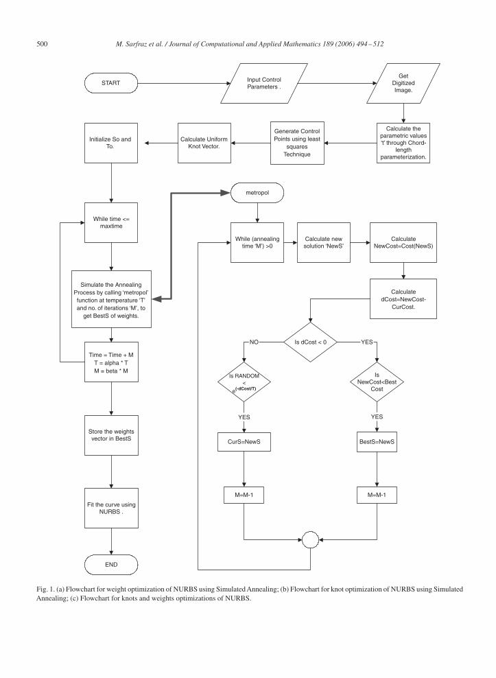
is the current weight corresponding to the control point (i), we calculate again the cost function E for the newly fittedcurve as NewCost. If the value of CurCost is less than NewCost, we assign the current cost value as the new cost andweight vector corresponding to this cost as the best solution (BestS). If the CurCost value is higher in comparison withNewCost, that means the perturb solution is worse than the original one. In this case, we accept the new solution onlyon probability basis i.e. a random number is generated between 0 and 1. If the generated random number is smallerthan e(CurCost−NewCost)/T , where T is the current temperature, then we keep the new settings. Otherwise, we neglect theperturb solution. This process is repeated slowly by decreasing the temperature until the optimized solution is reached.The flowchart for the NURBS curve approximation, based on SA, is shown in Fig. 1(a).
6.2. Knot optimization using SA
Knots can also be used, as parameters for optimization, in order to achieve better fitting accuracy. The error function(or cost function) between the measured points and the fitted curve is taken same as the function in weight optimizationshown in Eq. (5). The weight vector is set to unity.
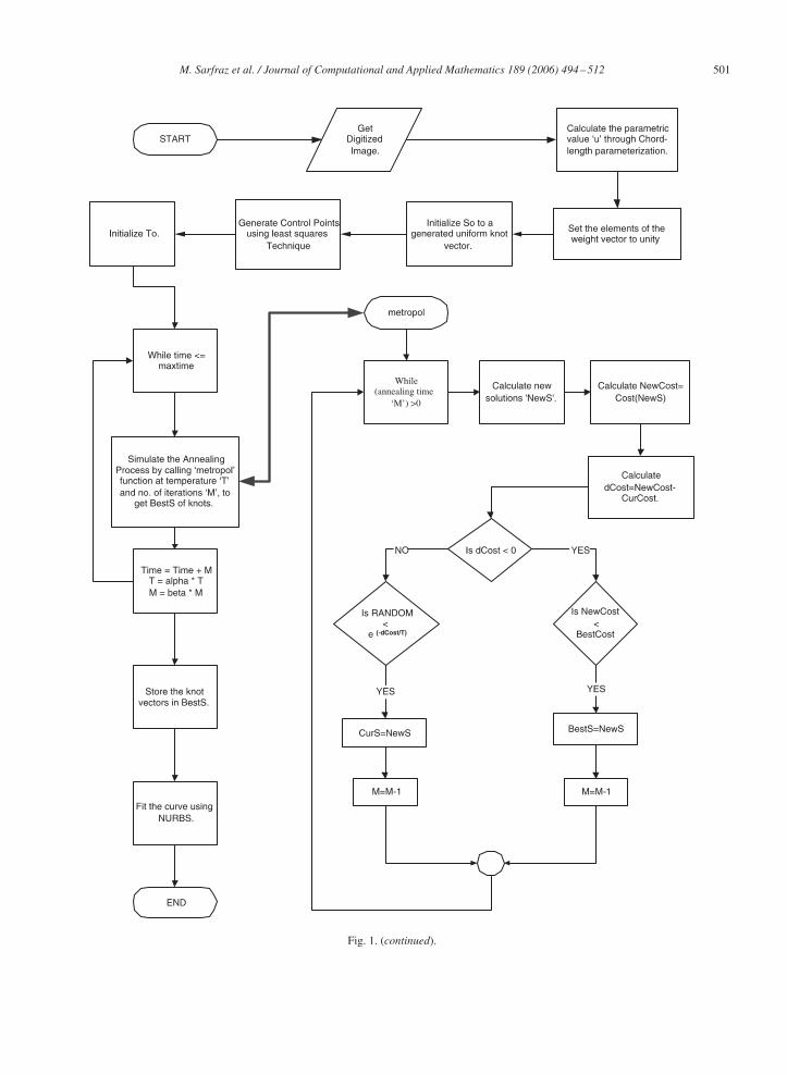
Knot optimization requires a good initial solution of knot vector. The initial solution S0 is a uniform knot vector,with a range of [0, npts (no. of control points) + k − 1]. The cooling schedule, in this scheme, is used in the samemanner as described in Section 6.1. The only change can be found in the knot vector perturbation. The perturbation ofthe current solution ‘CurS’ is generated in the neighborhood of [CurS − 0.001, CurS + 0.001]. The flowchart for theNURBS curve approximation, based on SA, is shown in Fig. 1(b).
6.3. Knot and weight optimization using SA
It is possible to combine the two optimizations in Sections 6.1 and 6.2. This can be done by optimizing the weightsand the knots simultaneously in order to get better curve approximation. We can consider a simply combined approachas follows: optimize the knots and then optimize the weights using the obtained knots. This way of knots and weights,as parameters for optimization, helps in order to achieve an improved fitting accuracy as compared to the methods ofSections 6.1 and 6.2. The error function (or cost function) between the measured points and the fitted curve is takensame as the function in weight optimization shown in Eq. (5). The weight vector is set to unity initially and initialsolution of knot vector is a uniform knot vector.
The cooling schedule, in this scheme, is used in the same manner as described in Sections 6.1 and 6.2. The flowchartfor the NURBS curve approximation, based on knots and weights optimization using SA, is shown in Fig. 1(c).
7. Results and discussion
This section is meant for the demonstrations of various results achieved during the implementations of the proposedschemes. Enough discussions are also made on the merits and demerits of the schemes.
500 M. Sarfraz et al. / Journal of Computational and Applied Mathematics 189 (2006) 494 –512
START Input ControlParameters .
Calculate theparametric values‘t’ through Chord-
lengthparameterization.
Initialize So andTo.
While time <=maxtime
Simulate the AnnealingProcess by calling ‘metropol’function at temperature ‘T’and no. of iterations ‘M’, to
get BestS of weights.
Time = Time + MT = alpha * TM = beta * M
Store the weightsvector in BestS
Fit the curve usingNURBS .
END
While (annealingtime ‘M’) >0
Calculate newsolution ‘NewS’
CalculateNewCost=Cost(NewS)
CalculatedCost=NewCost-
CurCost.
Is dCost < 0
Is RANDOM<
e(-dCost/T)
IsNewCost<Best
Cost
YESNO
BestS=NewS
YES
M=M-1
CurS=NewS
YES
M=M-1
metropol
Generate ControlPoints using least
squaresTechnique
Calculate UniformKnot Vector.
GetDigitizedImage.
Fig. 1. (a) Flowchart for weight optimization of NURBS using Simulated Annealing; (b) Flowchart for knot optimization of NURBS using SimulatedAnnealing; (c) Flowchart for knots and weights optimizations of NURBS.
M. Sarfraz et al. / Journal of Computational and Applied Mathematics 189 (2006) 494 –512 501
Fig. 1. (continued).
502 M. Sarfraz et al. / Journal of Computational and Applied Mathematics 189 (2006) 494 –512
Get digitized image
Extract contour points
Calculate the parametric values of NURBS
Calculate control points using least squares technique
Calculate the knot vector
Using SE, optimize knots and weights simultaneously
Fit the curve using optimized weights and knots for NURBS
START
END
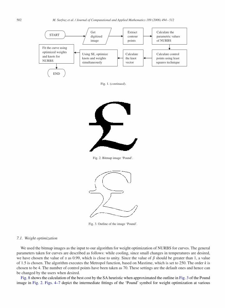
Fig. 1. (continued).
Fig. 2. Bitmap image ‘Pound’.
Fig. 3. Outline of the image ‘Pound’.
7.1. Weight optimization
We used the bitmap images as the input to our algorithm for weight optimization of NURBS for curves. The generalparameters taken for curves are described as follows: while cooling, since small changes in temperatures are desired,we have chosen the value of � as 0.99, which is close to unity. Since the value of � should be greater than 1, a valueof 1.5 is chosen. The algorithm executes the Metropol function, based on Maxtime, which is set to 250. The order k ischosen to be 4. The number of control points have been taken as 70. These settings are the default ones and hence canbe changed by the users when desired.
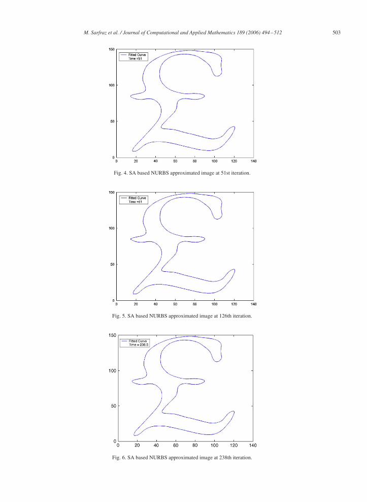
Fig. 8 shows the calculation of the best cost by the SA heuristic when approximated the outline in Fig. 3 of the Poundimage in Fig. 2. Figs. 4–7 depict the intermediate fittings of the ‘Pound’ symbol for weight optimization at various
M. Sarfraz et al. / Journal of Computational and Applied Mathematics 189 (2006) 494 –512 503
Fig. 4. SA based NURBS approximated image at 51st iteration.
Fig. 5. SA based NURBS approximated image at 126th iteration.
Fig. 6. SA based NURBS approximated image at 238th iteration.
504 M. Sarfraz et al. / Journal of Computational and Applied Mathematics 189 (2006) 494 –512
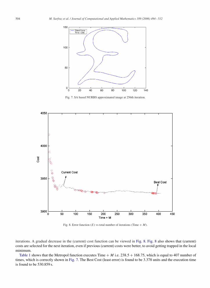
Fig. 7. SA based NURBS approximated image at 256th iteration.
Fig. 8. Error function (E) vs total number of iterations (Time + M).
iterations. A gradual decrease in the (current) cost function can be viewed in Fig. 8. Fig. 8 also shows that (current)costs are selected for the next iteration, even if previous (current) costs were better, to avoid getting trapped in the localminimum.
Table 1 shows that the Metropol function executes Time + M i.e. 238.5 + 168.75, which is equal to 407 number oftimes, which is correctly shown in Fig. 7. The Best Cost (least error) is found to be 3.378 units and the execution timeis found to be 530.859 s.
M. Sarfraz et al. / Journal of Computational and Applied Mathematics 189 (2006) 494 –512 505
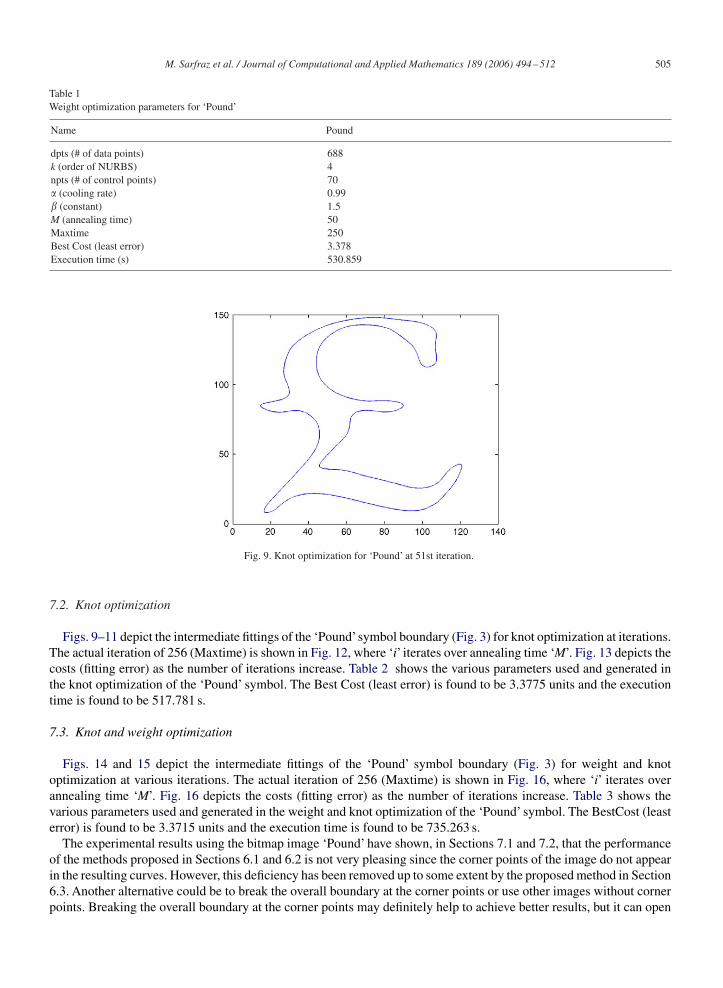
Table 1Weight optimization parameters for ‘Pound’
Name Pound
dpts (# of data points) 688k (order of NURBS) 4npts (# of control points) 70� (cooling rate) 0.99� (constant) 1.5M (annealing time) 50Maxtime 250Best Cost (least error) 3.378Execution time (s) 530.859
Fig. 9. Knot optimization for ‘Pound’ at 51st iteration.
7.2. Knot optimization
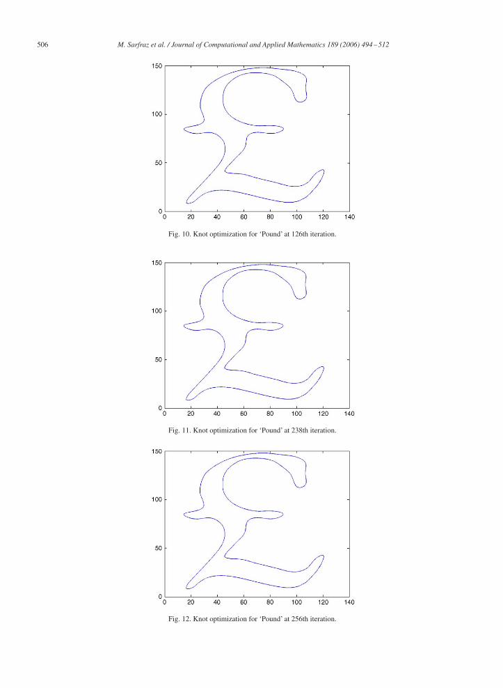
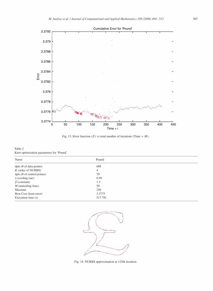
Figs. 9–11 depict the intermediate fittings of the ‘Pound’symbol boundary (Fig. 3) for knot optimization at iterations.The actual iteration of 256 (Maxtime) is shown in Fig. 12, where ‘i’ iterates over annealing time ‘M’. Fig. 13 depicts thecosts (fitting error) as the number of iterations increase. Table 2 shows the various parameters used and generated inthe knot optimization of the ‘Pound’ symbol. The Best Cost (least error) is found to be 3.3775 units and the executiontime is found to be 517.781 s.
7.3. Knot and weight optimization
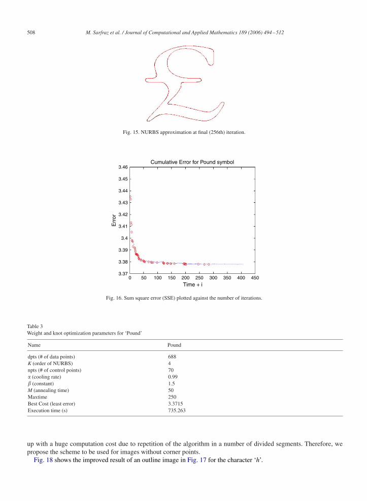
Figs. 14 and 15 depict the intermediate fittings of the ‘Pound’ symbol boundary (Fig. 3) for weight and knotoptimization at various iterations. The actual iteration of 256 (Maxtime) is shown in Fig. 16, where ‘i’ iterates overannealing time ‘M’. Fig. 16 depicts the costs (fitting error) as the number of iterations increase. Table 3 shows thevarious parameters used and generated in the weight and knot optimization of the ‘Pound’ symbol. The BestCost (leasterror) is found to be 3.3715 units and the execution time is found to be 735.263 s.
The experimental results using the bitmap image ‘Pound’ have shown, in Sections 7.1 and 7.2, that the performanceof the methods proposed in Sections 6.1 and 6.2 is not very pleasing since the corner points of the image do not appearin the resulting curves. However, this deficiency has been removed up to some extent by the proposed method in Section6.3. Another alternative could be to break the overall boundary at the corner points or use other images without cornerpoints. Breaking the overall boundary at the corner points may definitely help to achieve better results, but it can open
506 M. Sarfraz et al. / Journal of Computational and Applied Mathematics 189 (2006) 494 –512
Fig. 10. Knot optimization for ‘Pound’ at 126th iteration.
Fig. 11. Knot optimization for ‘Pound’ at 238th iteration.
Fig. 12. Knot optimization for ‘Pound’ at 256th iteration.
M. Sarfraz et al. / Journal of Computational and Applied Mathematics 189 (2006) 494 –512 507
3.3792
3.379
3.3788
3.3786
3.3784
3.3782
3.378
3.3778
3.3776
3.37740 50 100 150 200 250 300 350 400 450
Err
or
Time + i
Cumulative Error for 'Pound'
Fig. 13. Error function (E) vs total number of iterations (Time + M).
Table 2Knot optimization parameters for ‘Pound’
Name Pound
dpts (# of data points) 688K (order of NURBS) 4npts (# of control points) 70� (cooling rate) 0.99� (constant) 1.5M (annealing time) 50Maxtime 250Best Cost (least error) 3.3775Execution time (s) 517.781
Fig. 14. NURBS approximation at 125th iteration.
508 M. Sarfraz et al. / Journal of Computational and Applied Mathematics 189 (2006) 494 –512
Fig. 15. NURBS approximation at final (256th) iteration.
0
3.46
3.45
3.44
3.43
3.42
3.41
3.4
3.39
3.38
3.37
Err
or
Time + i
Cumulative Error for Pound symbol
50 100 150 200 250 300 350 400 450
Fig. 16. Sum square error (SSE) plotted against the number of iterations.
Table 3Weight and knot optimization parameters for ‘Pound’
Name Pound
dpts (# of data points) 688K (order of NURBS) 4npts (# of control points) 70� (cooling rate) 0.99� (constant) 1.5M (annealing time) 50Maxtime 250Best Cost (least error) 3.3715Execution time (s) 735.263
up with a huge computation cost due to repetition of the algorithm in a number of divided segments. Therefore, wepropose the scheme to be used for images without corner points.
Fig. 18 shows the improved result of an outline image in Fig. 17 for the character ‘h’.

M. Sarfraz et al. / Journal of Computational and Applied Mathematics 189 (2006) 494 –512 509
340
320
300
280
260
240
220
220 240 260 280 300 320 340 360
200
180
160
Boundary detection
Fig. 17. Outline image for the character ‘h’.
Fig. 18. NURBS approximation at final (256th) iteration.
Table 4Weight and knot optimization results summary, for the three proposed algorithms, using SA
Shapes Data points SA knot optimization SA weight optimization SA knot and weight optimization
Time Least error Time Least error Time Least error
Pound 688 517.781 3.3775 530.859 3.378 735.263 3.3715Aich 787 595.703 14.3 625.406 14.332 1166.371 14.31
7.4. Comparison and discussion
This paper has proposed three algorithms. The comparative study of these algorithms can be seen in Table 4. Thisstudy is done in terms of time and least error. The proposed algorthims are little different than that of Yoshimoto et al.[22]. They presented an algorithm for the determination of knots and their location was based on GA. But their workconsidered the case of non-parametric spline with no optimization of weight associated with control points.
Later, Raza [13] proposed a nested GA for parametric form of NURBS to optimize knots and weights separately. Butthe problem with that approach was the huge amount of execution time. The reason obviously could be the introductionof corner points in the description of the outline of the images used. The insertion of the corner points divides the wholecontour into a number of curve segments and hence causes the algorithm to be run number of times. The experimentalresults obtained using SA is found to be four times better than the results obtained using GA, in terms of the computation
510 M. Sarfraz et al. / Journal of Computational and Applied Mathematics 189 (2006) 494 –512
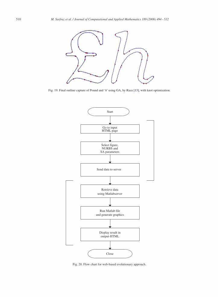
Fig. 19. Final outline capture of Pound and ‘h’ using GA, by Raza [13], with knot optimization.
Start
Go to inputHTML page
Select figure,NURBS and
SA parameters
Send data to server
Retrieve datausing Matlabserver
Run Matlab fileand generate graphics
Display result inoutput-HTML
Close
Fig. 20. Flow chart for web-based evolutionary approach.
M. Sarfraz et al. / Journal of Computational and Applied Mathematics 189 (2006) 494 –512 511
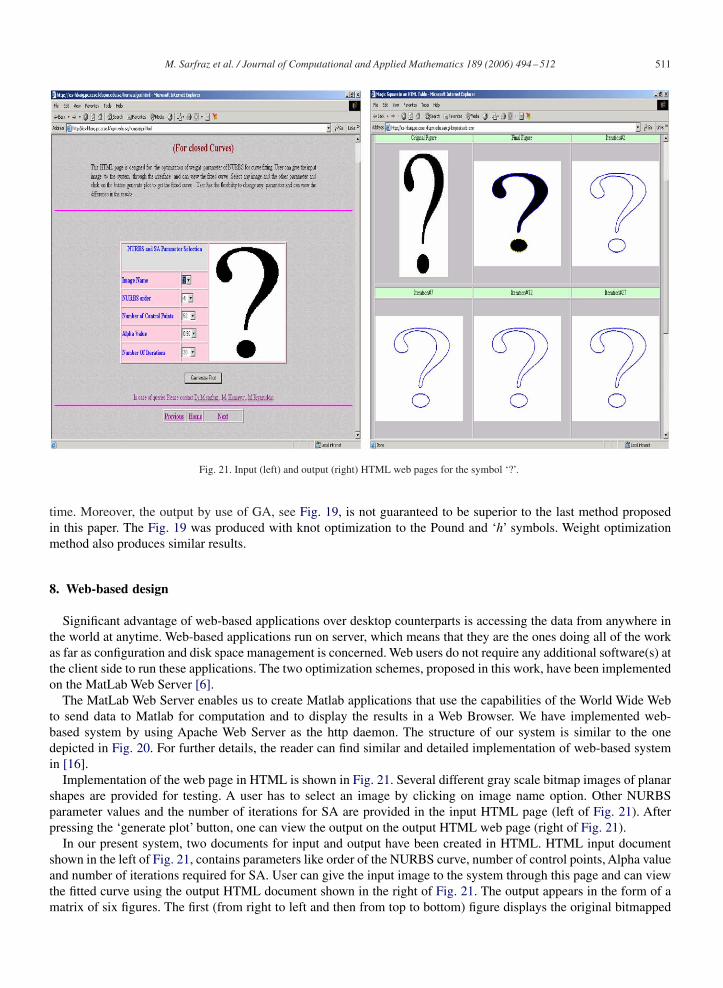
Fig. 21. Input (left) and output (right) HTML web pages for the symbol ‘?’.
time. Moreover, the output by use of GA, see Fig. 19, is not guaranteed to be superior to the last method proposedin this paper. The Fig. 19 was produced with knot optimization to the Pound and ‘h’ symbols. Weight optimizationmethod also produces similar results.
8. Web-based design
Significant advantage of web-based applications over desktop counterparts is accessing the data from anywhere inthe world at anytime. Web-based applications run on server, which means that they are the ones doing all of the workas far as configuration and disk space management is concerned. Web users do not require any additional software(s) atthe client side to run these applications. The two optimization schemes, proposed in this work, have been implementedon the MatLab Web Server [6].
The MatLab Web Server enables us to create Matlab applications that use the capabilities of the World Wide Webto send data to Matlab for computation and to display the results in a Web Browser. We have implemented web-based system by using Apache Web Server as the http daemon. The structure of our system is similar to the onedepicted in Fig. 20. For further details, the reader can find similar and detailed implementation of web-based systemin [16].
Implementation of the web page in HTML is shown in Fig. 21. Several different gray scale bitmap images of planarshapes are provided for testing. A user has to select an image by clicking on image name option. Other NURBSparameter values and the number of iterations for SA are provided in the input HTML page (left of Fig. 21). Afterpressing the ‘generate plot’ button, one can view the output on the output HTML web page (right of Fig. 21).
In our present system, two documents for input and output have been created in HTML. HTML input documentshown in the left of Fig. 21, contains parameters like order of the NURBS curve, number of control points, Alpha valueand number of iterations required for SA. User can give the input image to the system through this page and can viewthe fitted curve using the output HTML document shown in the right of Fig. 21. The output appears in the form of amatrix of six figures. The first (from right to left and then from top to bottom) figure displays the original bitmapped

512 M. Sarfraz et al. / Journal of Computational and Applied Mathematics 189 (2006) 494 –512
image, the second figure shows the digital outline detected, the rest of the images display the intermediate iterationresults together with the final result shown in the last figure.
9. Conclusion
A non-deterministic evolutionary approach, namely Simulated Annealing (SA), has been developed for approxi-mating the outlines of planar shapes. Non-uniform Rational B-splines (NURBS) have been utilized as an underlyingapproximation curve scheme. SA heuristic is used as an evolutionary methodology. In addition to independent studiesfor the optimization of weights and knots, a more effective scheme has been developed by combining the two inde-pendent studies. This scheme optimizes both weights and knots, simultaneously, of the NURBS model. The optimizedNURBS models have been fitted over the contour data of the planar shapes for the ultimate and automatic output. Theoutput results are visually pleasing with respect to the threshold provided by the user.
The scheme presented is web based for the worldwide utilization. MatLab Web Server has been used for the opti-mization of weight and knot parameters of NURBS for curve fitting on digital input obtained from scanned images orotherwise. Two HTML documents are designed to provide the input and to view the results. SA optimization heuristicalgorithm is used for the global optimization of the fitting error between a set of scanned points and a fitted curve.
Acknowledgements
The authors are thankful to the anonymous referees for their helpful and valuable suggestions towards the improve-ment of this manuscript. This work has been supported by King Fahd University of Petroleum and Minerals under thefunded project entitled “Reverse Engineering for Geometric Models using Evolutionary Heuristics”.
References
[1] J.J. Chou, L.A. Piegl, Data reduction using cubic rational B-splines, IEEE Comput. Graphics Appl. 1992.[2] D.E. Goldberg, Genetic algorithms in search, Optimization and Machine Learning, Addison-Wesley, Reading, MA, 1989.[3] M. Hoffmann, I. Juhasz, Shape control of cubic B-spline and NURBS curves by knot modifications, IEEE, 2001.[4] S. Kirkpatrick, C. Gelatt Jr., M. Vecchi, Optimization by Simulated Annealing, Science 220 (4598) (1983) 498–516.[5] A. Limaiem, A. Nassef, H.A. Elmaghraby, Data fitting using dual Krigging and Genetic Algorithms, CIRP Ann. 45 (1996) 129–134.[6] Matlab Web Server Manual, The math works Inc., 2000, 〈http://www.mathworks.com/access/helpdesk/help/pdf_doc/webserver/webserver.pdf〉[7] N. Metropolis, A. Roshenbluth, M. Rosenbluth, A. Teller, E. Teller, Equation of state calculations by fast computing machines, J. Chem. Phys.
21 (6) (1953) 1087–1092.[8] L. Piegl, On NURBS: a survey, IEEE Comput. Graphics Appl. 11 (1) (1991) 55–71.[9] L. Piegl, W. Tiller, The NURBS Book, Springer, Berlin, 1995.
[10] F. Pontrandolfo, G. Monno, A.E. Uva, Simulated Annealing vs Genetic Algorithms for linear spline approximation of 2D scattered data, XIIInternational Conference, Rimini, Italy, 2001.
[11] A. Quddus, Curvature analysis using multi-resolution techniques, Ph.D. Thesis, Department of Electric Engineering, King Fahd University ofPetroleum & Minerals, Dhahran, Saudi Arabia, 1998.
[12] S.S. Rao, Engineering Optimization, Theory and Practice, Wiley, New York, 1999.[13] S.A. Raza, Visualization with spline using a genetic algorithm, Master Thesis, King Fahd University of Petroleum & Minerals, Dhahran, Saudi
Arabia, 2001.[14] D.F. Rogers, An Introduction to NURBS With Historical Perspective, Morgan Kaufmann Publishers, Los Altos, CA, 2001.[15] M.S. Sait, H. Youssef, Iterative computer algorithms with applications in engineering: solving combinatorial optimization problems, IEEE
Computer Society Press, California, 1999.[16] M. Sarfraz, F.A. Razzak, A web based system to capture outline of Arabic fonts, Inform. Sci.-Informatics and Computer Science 150 (3–4)
(2003) 177–193.[17] B. Sarkar, C.H. Menq, Smooth surface approximation and reverse engineering, Comput. Aided Design 23 (1991) 623–628.[18] B. Sarkar, C.H. Menq, Parameter optimization in approximating curves and surfaces to measurement data, Comput. Aided Geom. Design 8
(1991) 267–290.[19] M.M. Shalaby, A.O. Nassef, S.M. Metwalli, On the classification of fitting problems for single patch free-form surfaces in reverse engineering,
Proceedings of the ASME Design Automation Conference, Pittsburgh, 2001b.[20] H. Xie, H. Qin, Automatic knot determination of NURBS for interactive geometric design, IEEE, 2001.[21] H.T. Yau, J.S. Chen, Reverse engineering of complex geometry using rational B-splines, Internat. J. Adv. Manufac. Tech. 13 (1997) 548–555.[22] Y. Yoshimoto, M. Moriyama, T. Harada, Automatic knot replacement by a genetic algorithm for data fitting with a spline, shape modeling and
applications, 1999, Proceedings of the International Conference—Shape Modeling International ’99. 1–4 March, 1999, pp. 162–169.[23] A.M. Youssef, Reverse engineering of geometric surfaces using Tabu search optimization technique, Master Thesis, Cairo University, Egypt,
2001.