A unified approach for parameterizing the boundary layer and moist convection

A unified approach for parameterizing the boundary layer and moist convection

Cara-Lyn LappenColorado State University

Cara-Lyn LappenColorado State University

OUTLINEWhy unified models?ADHOCLateral mixing and sub-plume fluxesModel versatilityADHOC2/Momentum fluxesParting wisdom

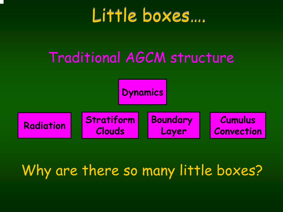
Little boxes….Little boxes….

Traditional AGCM structure

Dynamics

Radiation StratiformClouds

BoundaryLayer

CumulusConvection

Why are there so many little boxes?

QuickTime™ and aCinepak decompressor

are needed to see this picture.

QuickTime™ and aCinepak decompressor

are needed to see this picture.

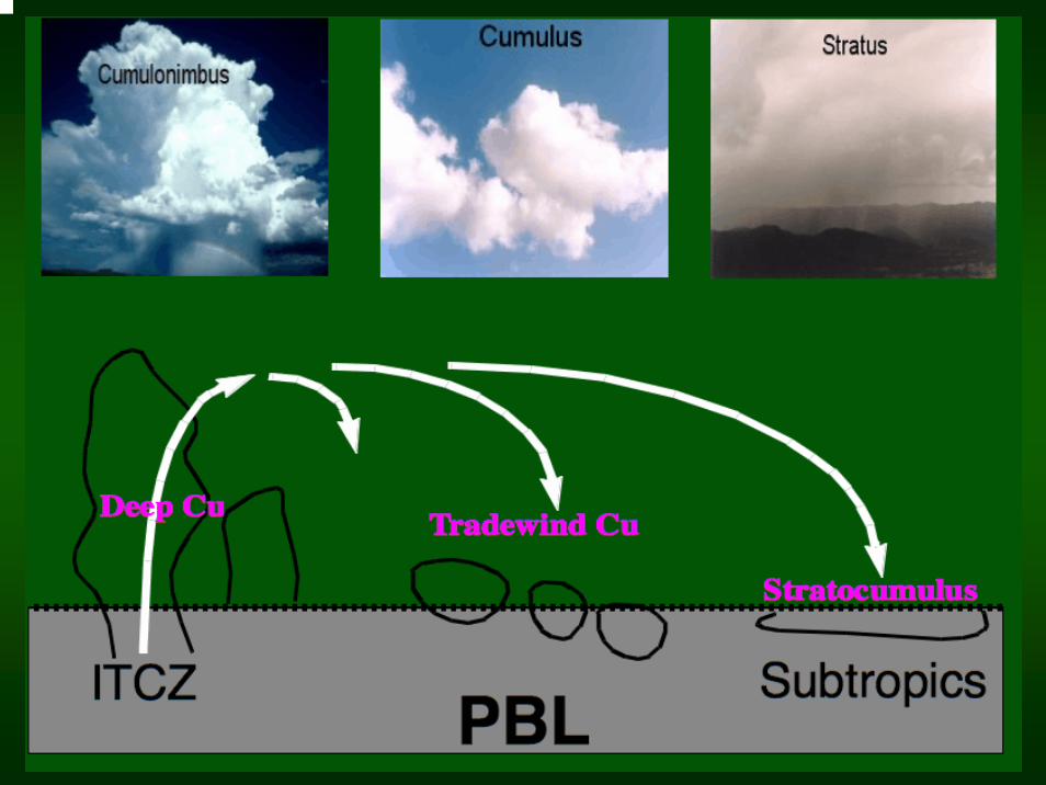
Its all really just fluid flow…

isnt it?

Its all really just fluid flow…

isnt it?

*Movies courtesy of Marat Khairoutinov’s RICO simulations

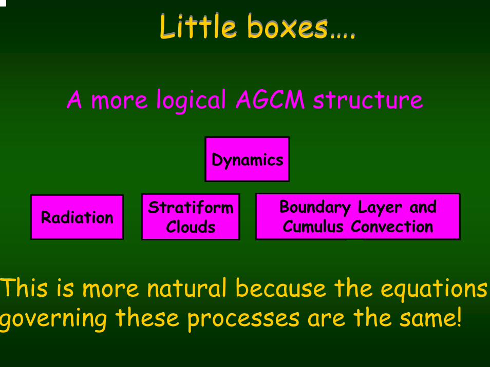
Little boxes….Little boxes….

A more logical AGCM structure

Dynamics

Radiation StratiformClouds

BoundaryLayer

CumulusConvection

This is more natural because the equationsgoverning these processes are the same!

Dynamics

Radiation StratiformClouds

Boundary Layer and Cumulus Convection

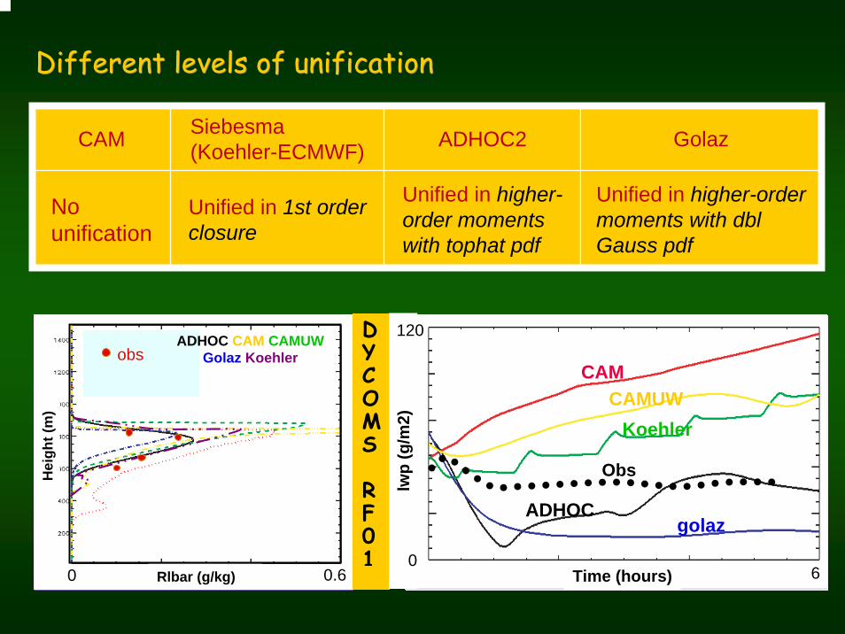
Different levels of unificationDifferent levels of unification

CAM Siebesma(Koehler-ECMWF) ADHOC2 Golaz

No unification

Unified in 1st order closure

Unified in higher-order moments with tophat pdf

Unified in higher-order moments with dbl Gauss pdf

obsADHOC CAM CAMUW

Golaz Koehler

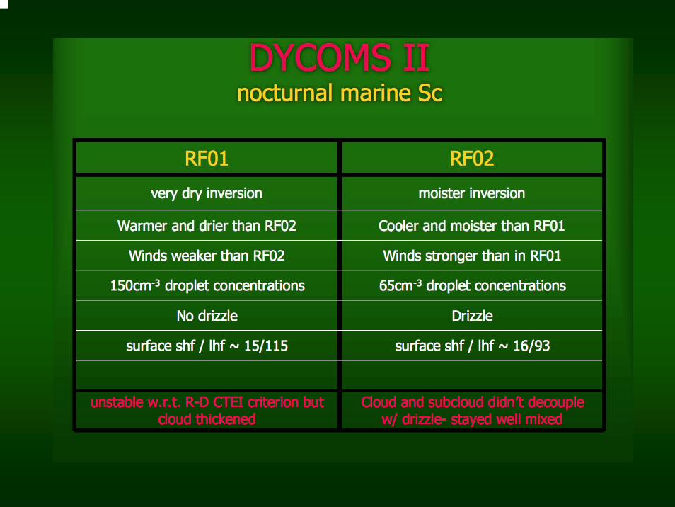
DYCOMS

RF01

0.60 Rlbar (g/kg)

Hei

ght (

m)

CAMUWCAM

Koehler

ADHOCgolaz

Obs

Time (hours)

lwp

(g/m

2)

120

06

ADHOCADHOCAmateurs Doing Higher Order Closure

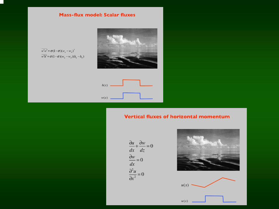
w = σwup + (1− σ )wdn

′w ′w = σ (1− σ )(wup − wdn )2′w ′w = σ (1− σ )(wup − wdn )2

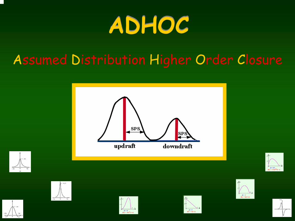
ADHOCADHOCAssumed Distribution Higher Order Closure

Randall et al. (1992)

′w ′w = σ (1− σ )(wup − wdn )2′w ′w = σ (1− σ )(wup − wdn )2

w = σ w up + (1 − σ )w dn

′w ′w ′w = σ (1− σ )(1− 2σ )(wup − wdn )3

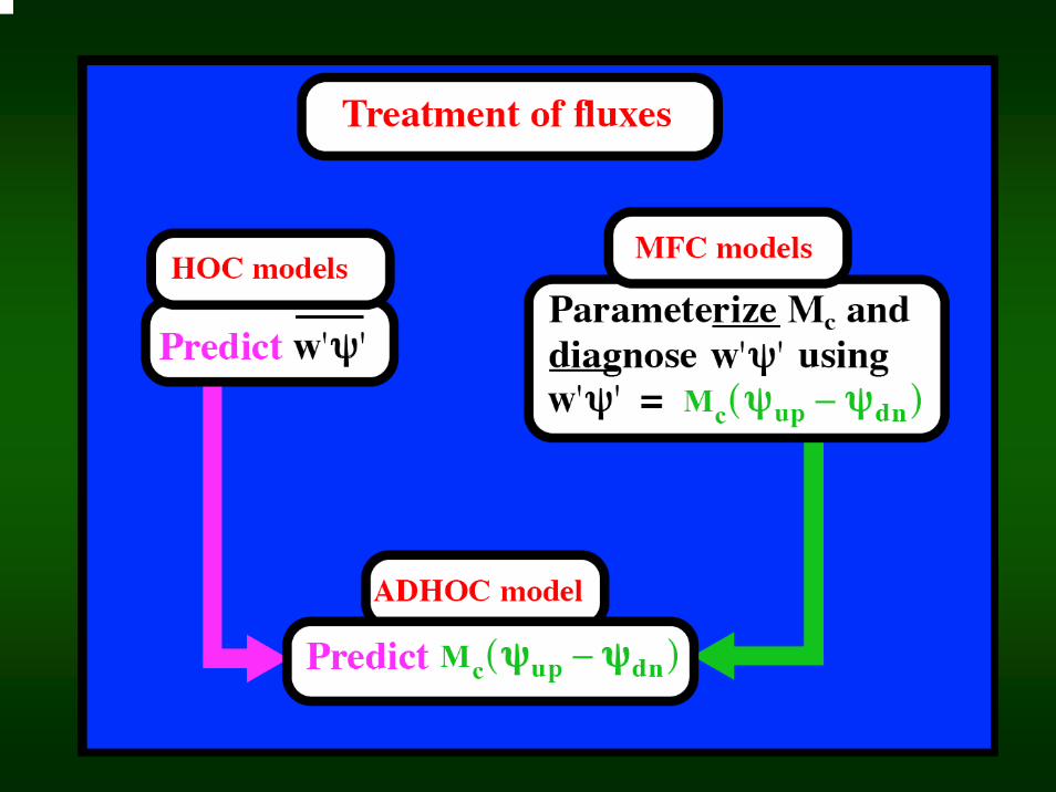
Solving, we can diagnose the mass flux:

Mc = ρσ (1− σ )(wup − wdn )

}σ 1 − σ}

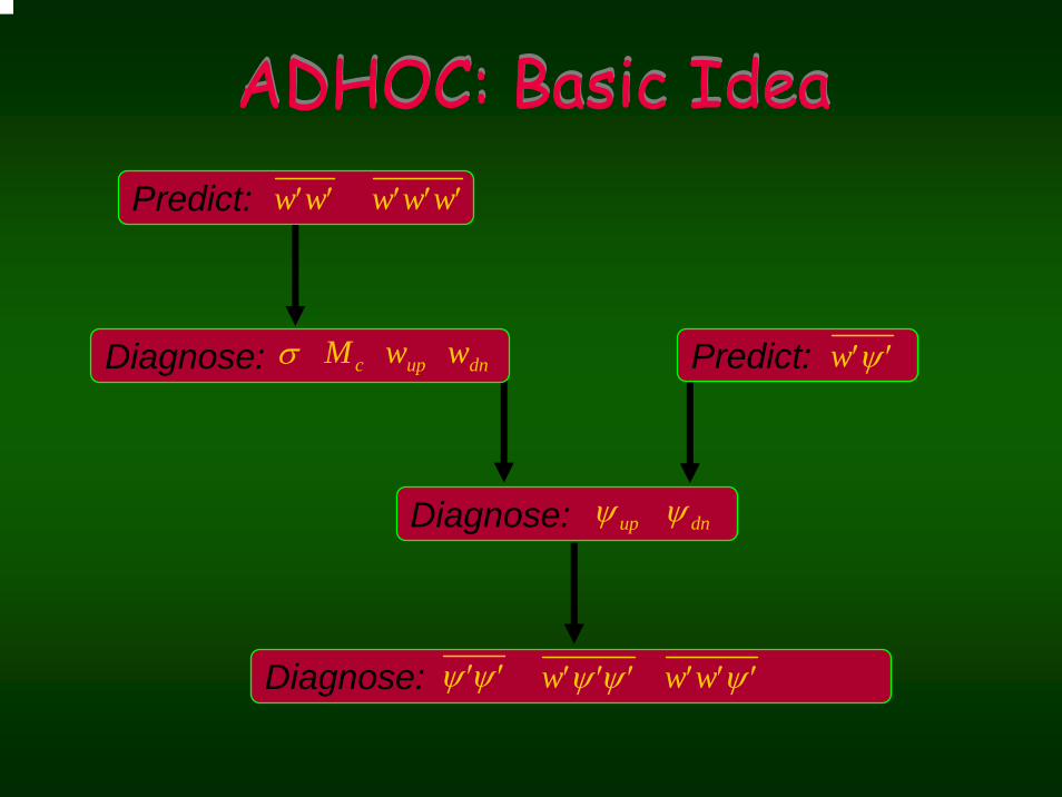
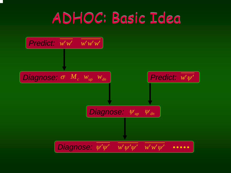
ADHOC: Basic IdeaADHOC: Basic Idea

• • • • •

Predict: ′w ′w ′w ′w ′w

Predict: ′w ′ψDiagnose: σ Mc wup wdn

Diagnose: ψ up ψ dn

Diagnose: ′ψ ′ψ ′w ′ψ ′ψ ′w ′w ′ψ

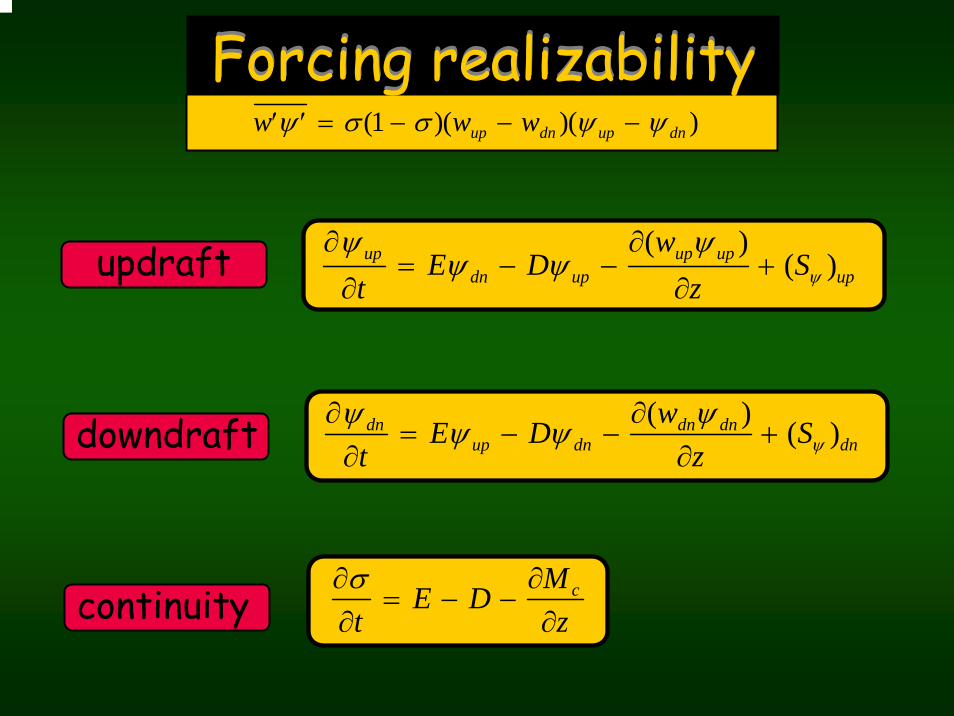
Forcing realizabilityForcing realizability

∂σ∂t

= E − D −∂Mc

∂zcontinuity

∂ψ dn

∂t= Eψ up − Dψ dn −

∂(wdnψ dn )∂z

+ (Sψ )dndowndraft

∂ψ up

∂t= Eψ dn − Dψ up −

∂(wupψ up )∂z

+ (Sψ )upupdraft

′w ′ψ = σ (1 − σ )(wup − wdn )(ψ up − ψ dn )

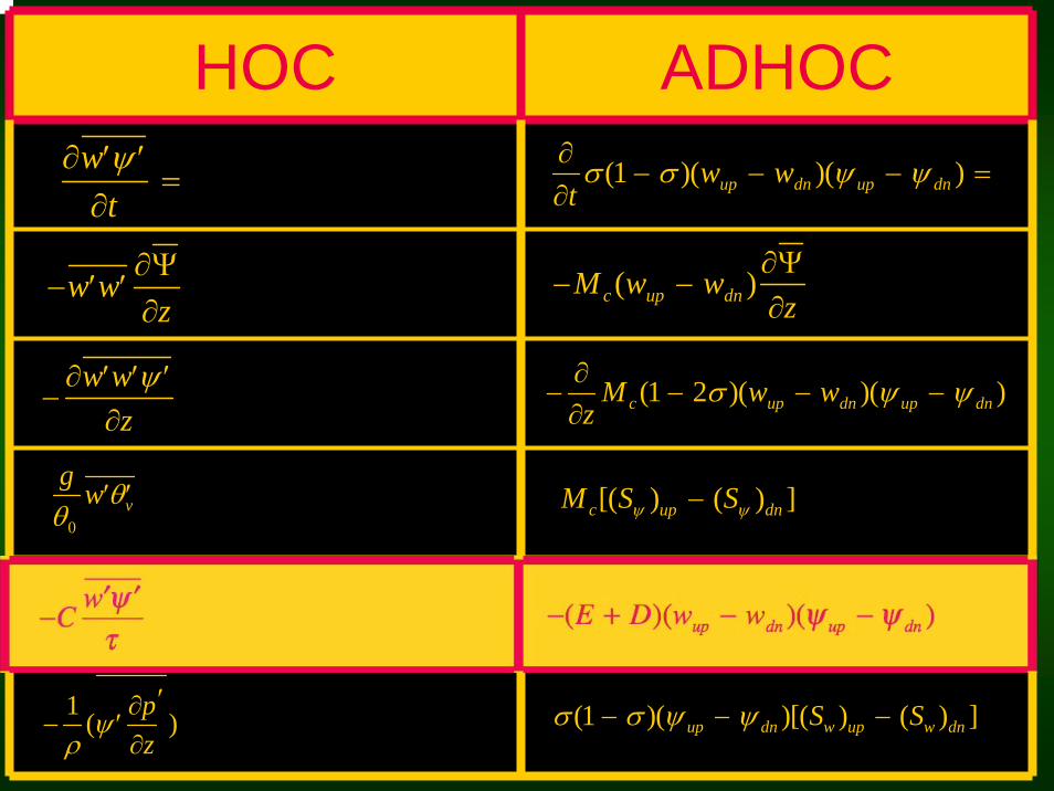
HOC ADHOC

−C ′w ′ψτ

−(E + D)(wup − wdn )(ψ up − ψ dn )

gθ0

′w ′θv

σ (1 − σ )(ψ up − ψ dn )[(Sw )up − (Sw )dn ]

∂ ′w ′ψ∂t

=∂∂tσ (1 − σ )(wup − wdn )(ψ up − ψ dn ) =

− ′w ′w∂Ψ∂z

−Mc (wup − wdn )∂Ψ∂z

−∂ ′w ′w ′ψ

∂z−∂∂z

Mc (1 − 2σ )(wup − wdn )(ψ up − ψ dn )

−1ρ

( ′ψ∂p∂z

′)

Mc[(Sψ )up − (Sψ )dn ]

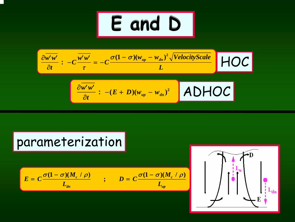
E and DE and D∂ ′w ′w∂t

: −C ′w ′wτ

= −Cσ (1 − σ )(wup − wdn )2 VelocityScale

L HOC∂ ′w ′w∂t

: −(E + D)(wup − wdn )2 ADHOC

E = Cσ (1 − σ )(Mc / ρ)

Ldn

; D = Cσ (1 − σ )(Mc / ρ)

Lup

parameterization

ADHOC: Basic IdeaADHOC: Basic IdeaPredict: ′w ′w ′w ′w ′w

Predict: ′w ′ψDiagnose: σ Mc wup wdn

Diagnose: ψ up ψ dn

Diagnose: ′ψ ′ψ ′w ′ψ ′ψ ′w ′w ′ψ • • • • •

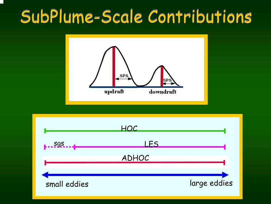
small eddies large eddies

LES

HOC

MF

SubPlume-Scale ContributionsSubPlume-Scale Contributions

sgs

sps ADHOC

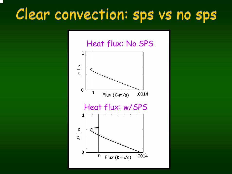
zzi

zzi

1

Heat flux: No SPS

Clear convection: sps vs no spsClear convection: sps vs no sps

Heat flux: w/SPSFlux (K-m/s)

1

0 0

00

.0014

.0014

Flux (K-m/s)

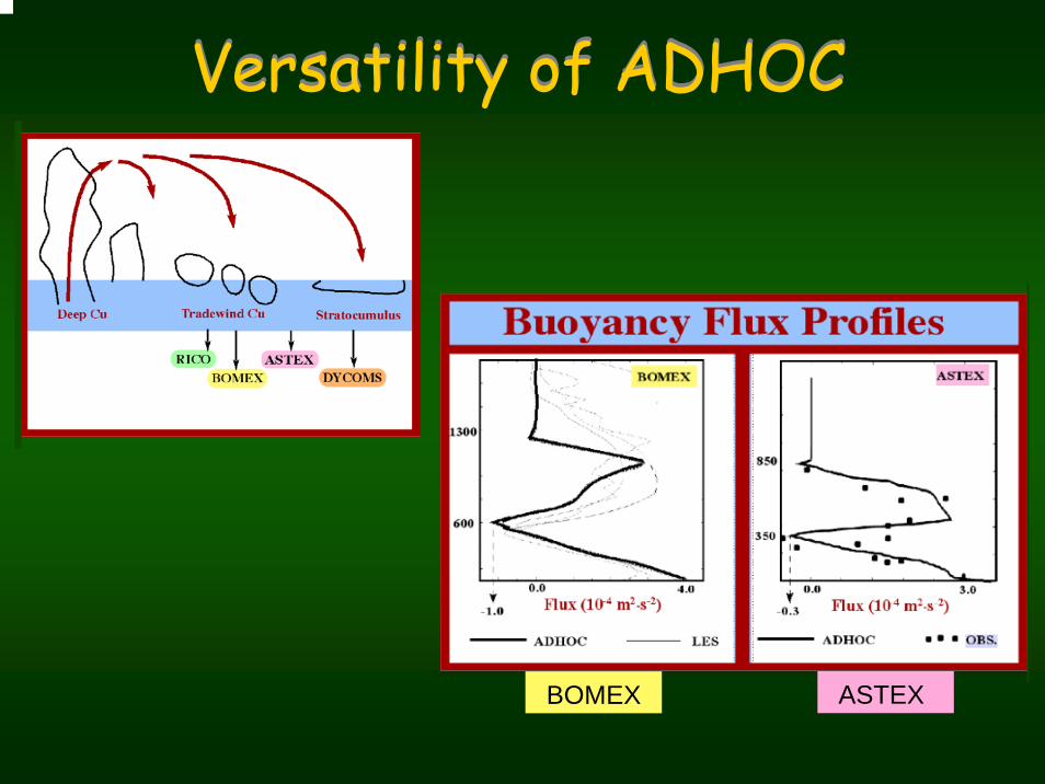
Versatility of ADHOCVersatility of ADHOC

BOMEX ASTEX

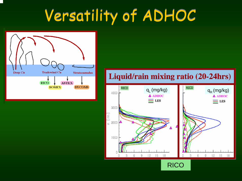
Versatility of ADHOCVersatility of ADHOC

RICO

qL (mg/kg) qR (mg/kg)

Versatility of ADHOCVersatility of ADHOC

DYCOMSg/kgg/kg 0.500.60

ADHOC2ADHOC2

ADHOC: Basic IdeaADHOC: Basic IdeaPredict: ′w ′w ′w ′w ′w

Predict: ′w ′ψDiagnose: σ Mc wup wdn

Diagnose: ψ up ψ dn

Diagnose: ′ψ ′ψ ′w ′ψ ′ψ ′w ′w ′ψ • • • • •

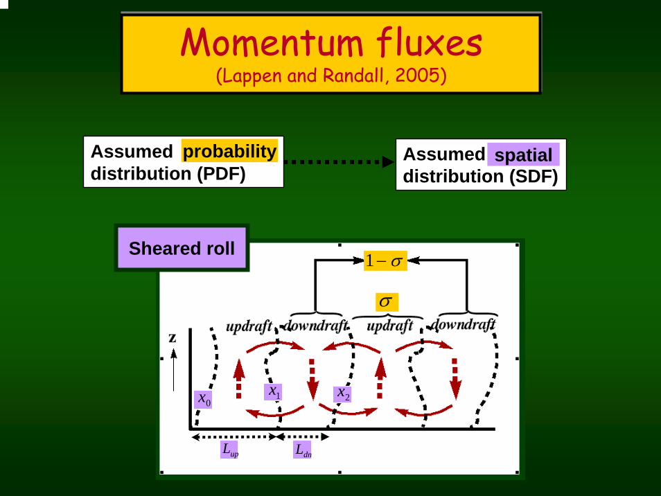
Momentum fluxes(Lappen and Randall, 2005)

Momentum fluxes(Lappen and Randall, 2005)

Assumed distribution (PDF)

probability Assumed distribution (SDF)

spatial

x0x1 x2

LdnLupLup Ldn

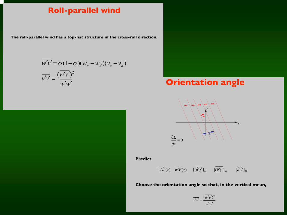
Sheared roll 1− σ

σ

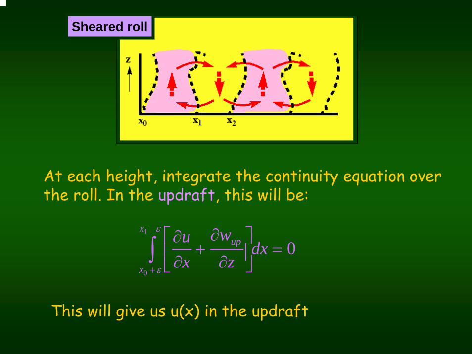
At each height, integrate the continuity equation over the roll. In the updraft, this will be:

∂u∂x

+∂wup

∂z⎡

⎣⎢

⎤

⎦⎥

x0 +ε

x1 −ε

∫ dx = 0

This will give us u(x) in the updraft

Sheared roll

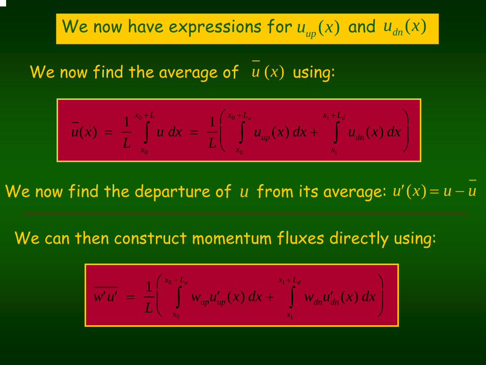
We now find the average of using:u (x)

u(x) =1L

u dxx0

x0 +L

∫ =1L

uup (x) dx + udn (x) dxx1

x1 +Ld

∫x0

x0 +Lu

∫⎛

⎝⎜

⎞

⎠⎟

′u (x) = u − uWe now find the departure of from its average:u

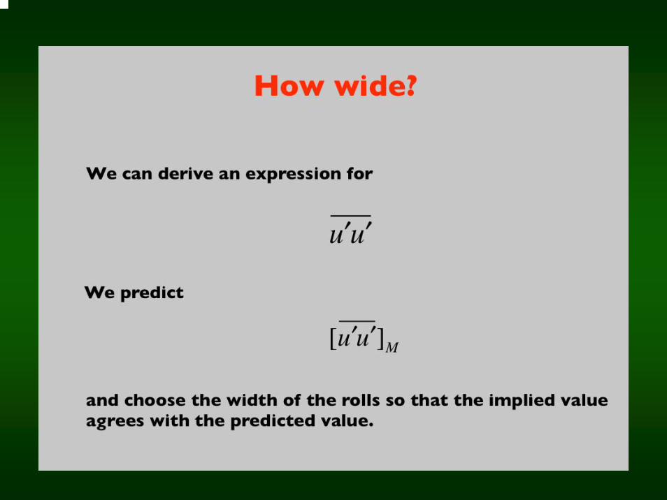
We can then construct momentum fluxes directly using:

′w ′u =1L

wup ′uup (x) dx + wdn ′udn (x) dxx1

x1 +Ld

∫x0

x0 +Lu

∫⎛

⎝⎜

⎞

⎠⎟

We now have expressions for anduup (x) udn (x)

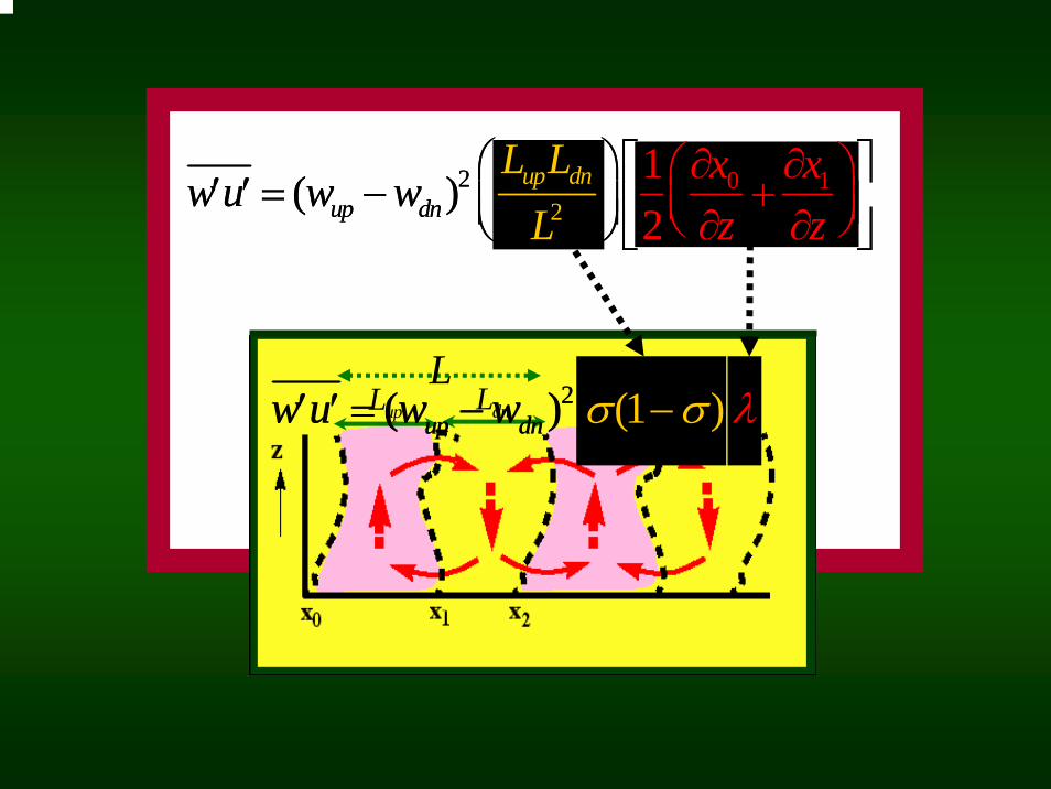
′w ′u = (wup −wdn)2 LupLdn

L2

⎛⎝⎜

⎞⎠⎟

12

∂x0

∂z+∂x1

∂z⎛⎝⎜

⎞⎠⎟

⎡

⎣⎢

⎤

⎦⎥

Lup Ldn

L′w ′u = (wup −wdn)

2 σ(1−σ) λ′w ′u = (wup −wdn)2 σ(1−σ) λ

′w ′u = (wup −wdn)2 LupLdn

L2

⎛⎝⎜

⎞⎠⎟

12

∂x0

∂z+∂x1

∂z⎛⎝⎜

⎞⎠⎟

⎡

⎣⎢

⎤

⎦⎥

′u ′u =13

Lσ(1−σ)∂(wup −wdn)

∂z⎡

⎣⎢

⎤

⎦⎥

2

+

13

Lσ(1−σ)∂(wup −wdn)

2

∂z(1−2σ)L

∂σ∂z

+ 4σ(1−σ)λ⎡⎣⎢

⎤⎦⎥+

′w ′u λ+(1−2σ)

2L∂σ∂z

⎡⎣⎢

⎤⎦⎥+ (wup −wdn)L

∂σ∂z

⎡⎣⎢

⎤⎦⎥

2 1− 3σ + 3σ2

2⎛⎝⎜

⎞⎠⎟

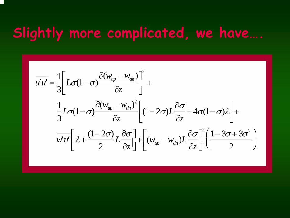
Slightly more complicated, we have….

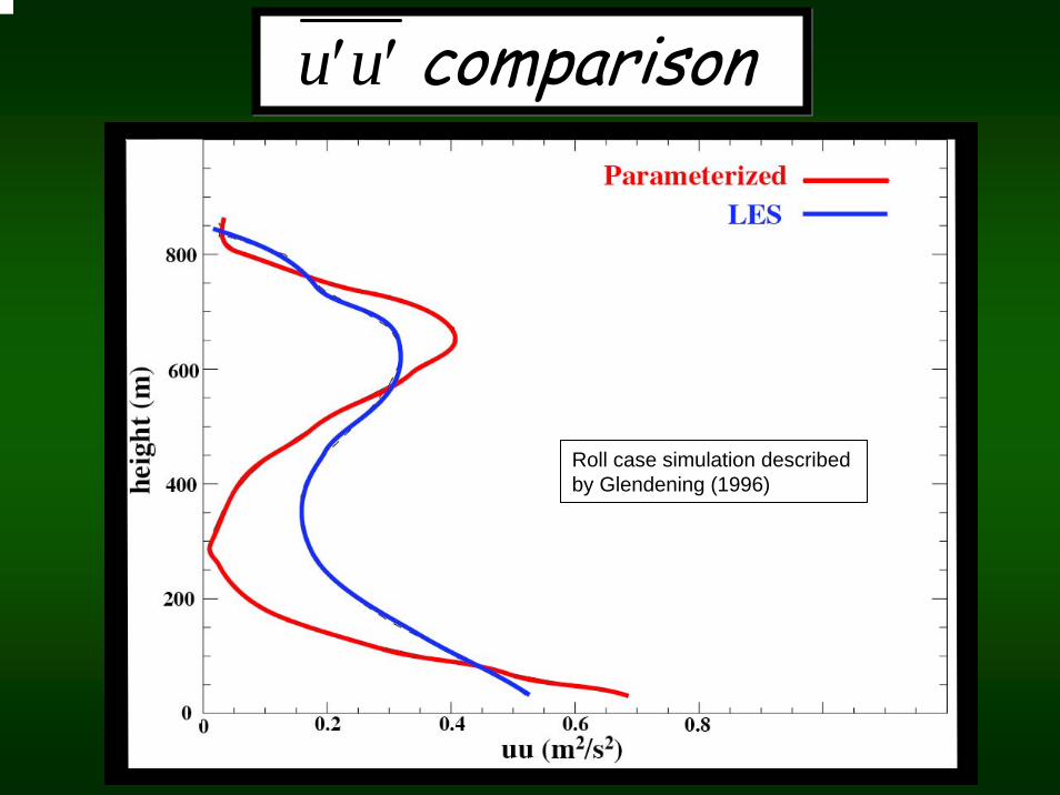
comparison--comparison--′u ′u

Roll case simulation describedby Glendening (1996)

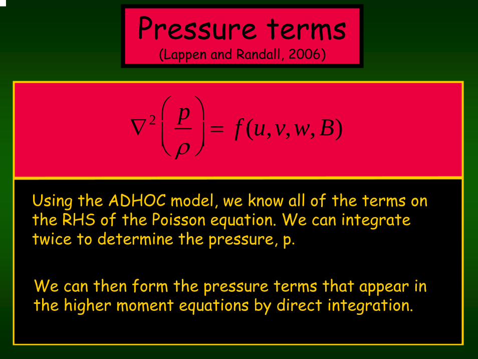
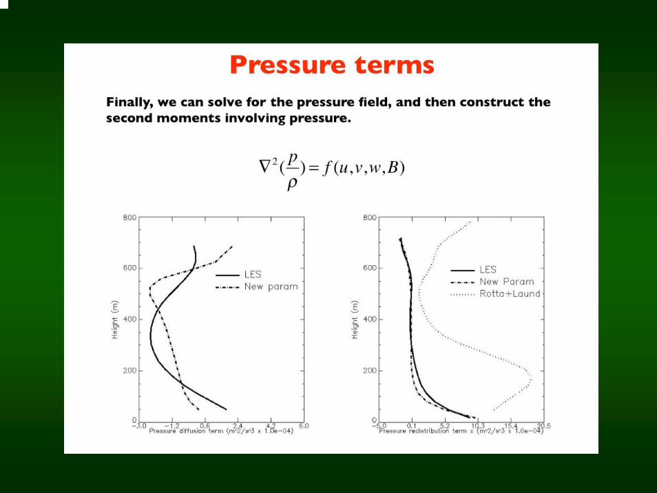
Pressure terms(Lappen and Randall, 2006)

∇2 pρ

⎛⎝⎜

⎞⎠⎟= f (u,v,w, B)

Using the ADHOC model, we know all of the terms on the RHS of the Poisson equation. We can integrate twice to determine the pressure, p.

We can then form the pressure terms that appear in the higher moment equations by direct integration.

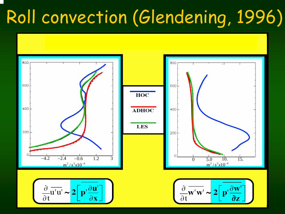
Roll convection (Glendening, 1996)

m2 / s3x10−431.2−0.6−2.4−4.2

m2 / s3x10−40 5.0 10. 15.

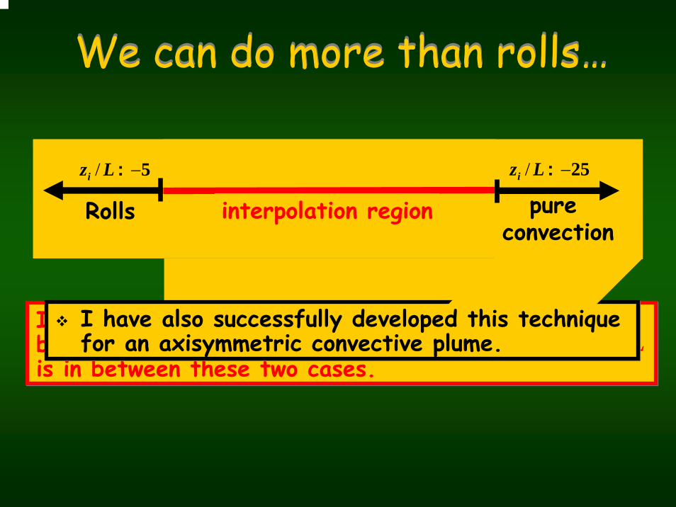
Rolls

zi / L : −5

We can do more than rolls…We can do more than rolls…

I have started research to use a Richardson-number based interpolation to represent convection whose is in between these two cases.

I have started research to use a Richardson-number based interpolation to represent convection whose is in between these two cases.

interpolation region

zi / LI have also successfully developed this technique for an axisymmetric convective plume.I have also successfully developed this technique for an axisymmetric convective plume.

pure convection

zi / L : −25

Transitional regimes are more naturally represented.and are determined from the physics of the flow.

There are no realizability issues with higher moments.A natural method to represent lateral mixing emerges.

Criterion used to define updrafts not important becausewe have an SPS model.

Momentum fluxes can be determined within the same framework by combining the mass-flux PDF with an SDF.

The pressure field and the pressure terms in the 2nd moment equations can be calculated directly.

ADHOC has successfully simulated a range of PBLs from the tropics through the subtropics

Summary

σ Mc

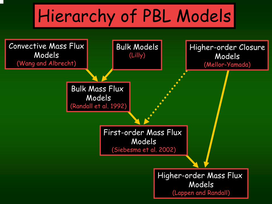
Convective Mass FluxModels

(Wang and Albrecht)

Bulk Models(Lilly)

Higher-order ClosureModels

(Mellor-Yamada)

Bulk Mass FluxModels

(Randall et al. 1992)

Higher-order Mass FluxModels

(Lappen and Randall)

First-order Mass FluxModels

(Siebesma et al. 2002)

Hierarchy of PBL Models

After all,its all just fluid flow,

…..isnt it?

After all,its all just fluid flow,

…..isnt it?

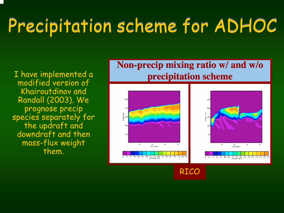
Precipitation scheme for ADHOCPrecipitation scheme for ADHOC

I have implemented a modified version ofKhairoutdinov and

Randall (2003). We prognose precip

species separately for the updraft and

downdraft and then mass-flux weight

them.

RICO

New ADHOC-consistent momentum flux parameterization (Lappen and Randall, 2005)

New ADHOC-consistent pressure term parameterization (Lappen and Randall, 2006)

A few new prognostic equations

New ADHOC-consistent microphysics

New ADHOC-consistent momentum flux parameterization (Lappen and Randall, 2005)

New ADHOC-consistent pressure term parameterization (Lappen and Randall, 2006)

A few new prognostic equations

New ADHOC-consistent microphysics

Whats new in ADHOC2?

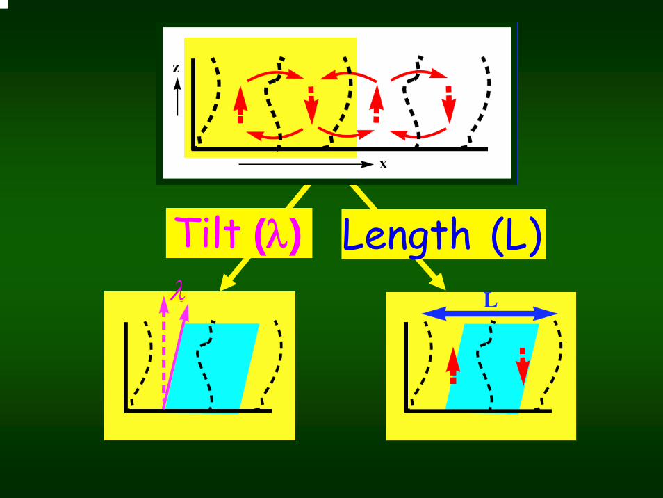
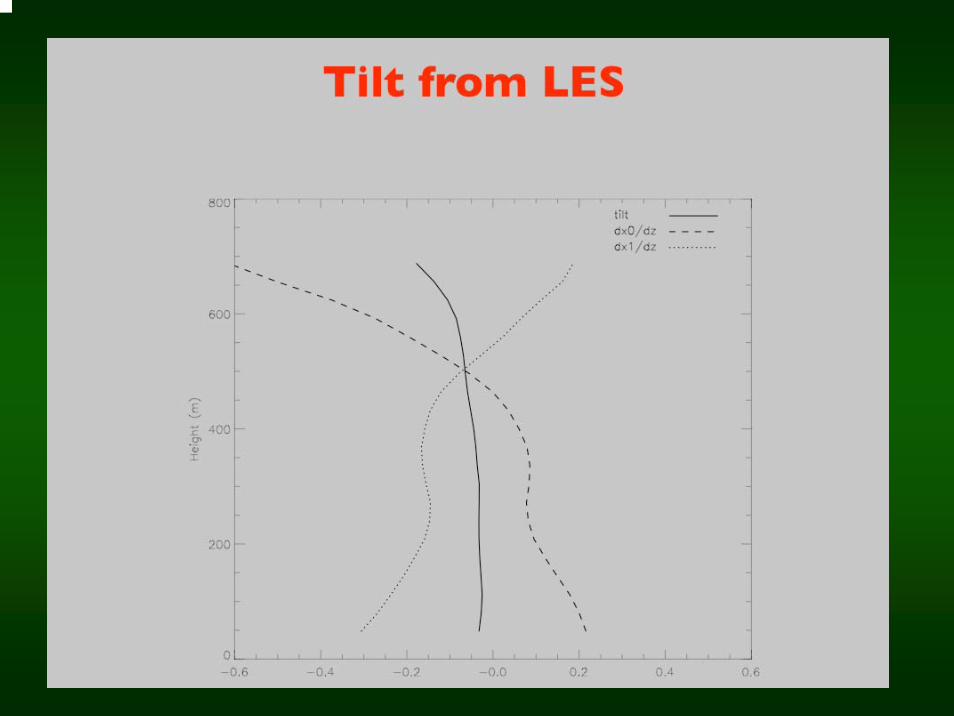
λ

Tilt (λ) Length (L)

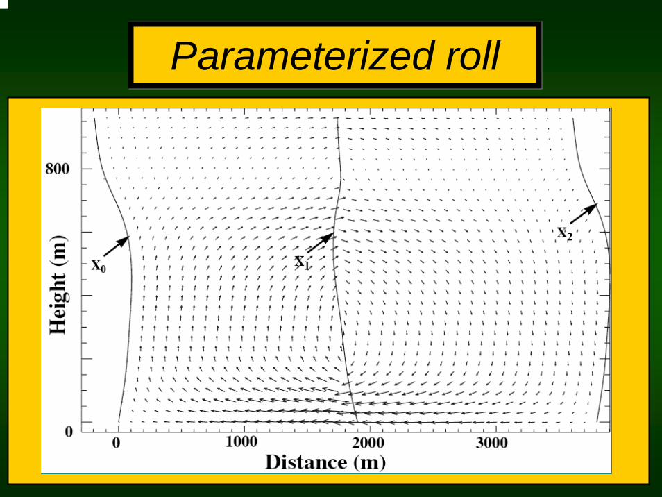
Parameterized rollParameterized roll

Summary of new research

The 3-D roll circulation

The tilt

The wavelength

The orientation angle

The pressure field and the pressure termsin the 2nd moment equations

The 3-D roll circulation

The tilt

The wavelength

The orientation angle

The pressure field and the pressure termsin the 2nd moment equations

From the predicted values of ADHOC2, we can determine:

Using parameters of the spatial distribution of the flow (SDF), momentum fluxes can be incorporated into a mass-flux model in a manner consistent with the thermodynamic fluxes

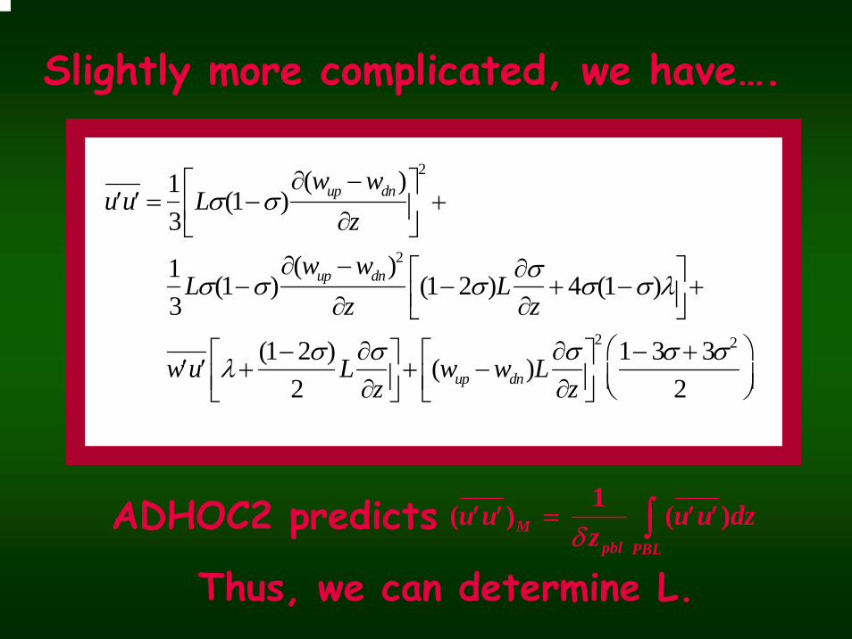
′u ′u =13

Lσ(1−σ)∂(wup −wdn)

∂z⎡

⎣⎢

⎤

⎦⎥

2

+

13

Lσ(1−σ)∂(wup −wdn)

2

∂z(1−2σ)L

∂σ∂z

+ 4σ(1−σ)λ⎡⎣⎢

⎤⎦⎥+

′w ′u λ+(1−2σ)

2L∂σ∂z

⎡⎣⎢

⎤⎦⎥+ (wup −wdn)L

∂σ∂z

⎡⎣⎢

⎤⎦⎥

2 1− 3σ + 3σ2

2⎛⎝⎜

⎞⎠⎟

Slightly more complicated, we have….

ADHOC2 predicts ( ′u ′u )M =1

δ zpbl

( ′u ′uPBL∫ )dz

Thus, we can determine L.

( ′u ′u )M = ′u ′uPBL∫ dz

ADHOC2: Basic idea

Predict: ( ′u ′v )M ( ′v ′v )M( ′u ′u )MDiagnose: ′u ′u ′v ′v′u ′v

Diagnose: L

Diagnose: ′w ′w ′u ′w ′w ′v •••••

Diagnose: λ η

Predict: ′w ′u ′w ′v

( ′u ′u )M = ′u ′uPBL∫ dz

ADHOC2: Basic idea

Predict: ( ′u ′v )M ( ′v ′v )M( ′u ′u )MDiagnose: ′u ′u ′v ′v′u ′v

Diagnose: ′w ′w ′u ′w ′w ′v •••••

Predict: ′w ′u ′w ′v

Diagnose: λ η L

x0x1 x2

LdnLupLup Ldn

σ

1 − σ

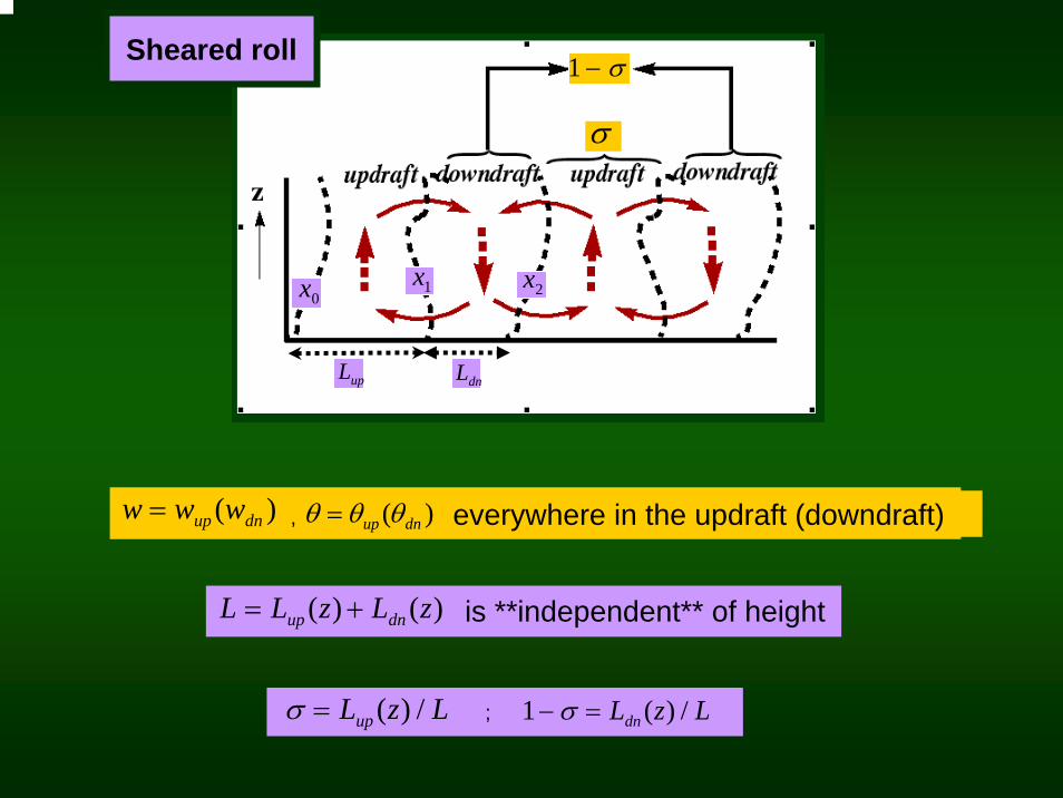
w = wup (wdn ) , θ = θup (θdn ) everywhere in the updraft (downdraft)

σ = Lup (z) / L ; 1− σ = Ldn (z) / L

L = Lup (z) + Ldn (z) is **independent** of height

Sheared roll

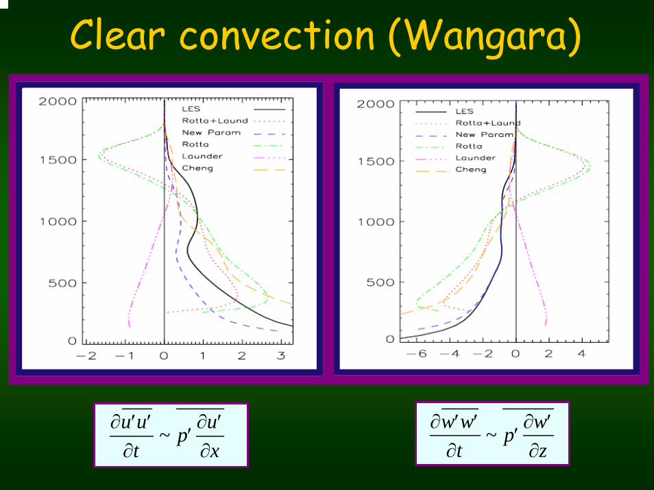
∂ ′u ′u∂t

~ ′p∂ ′u∂x

∂ ′w ′w∂t

~ ′p∂ ′w∂z

Clear convection (Wangara)

Transitional regimes are more naturally represented

and are determined from the physics of the flow.

There are no realizability issues with higher moments.

A natural method to represent lateral mixing emerges.

Criterion used to define updrafts not important because we have an SPS model

Momentum fluxes can be determined within the same framework.

Advantages of ADHOC

σ Mc