ICARUS 126, 324–335 (1997)ARTICLE NO. IS965655

Carbon Monoxide in Jupiter after Comet Shoemaker–Levy 9

KEITH S. NOLL1 AND DIANE GILMORE1

Space Telescope Science Institute, 3700 San Martin Drive, Baltimore, Maryland 21218E-mail: noll@stsci.edu

ROGER F. KNACKE1 AND MARIA WOMACK

Pennsylvania State University, Erie, Pennsylvania 16563

CAITLIN A. GRIFFITH1

Northern Arizona University, Flagstaff, Arizona 86011

AND

GLENN ORTON1

Jet Propulsion Laboratory, Pasadena, California 91109

Received February 5, 1996; revised November 5, 1996

for roughly half the mass. In high-temperature shocks,most of the O is converted to CO (Zahnle and MacLowObservations of the carbon monoxide fundamental vibra-

tion–rotation band near 4.7 mm before and after the impacts 1995), making CO one of the more abundant products ofof the fragments of Comet Shoemaker–Levy 9 showed no de- a large impact.tectable changes in the R5 and R7 lines, with one possible By contrast, oxygen is a rare element in Jupiter’s upperexception. Observations of the G-impact site 21 hr after impact atmosphere. The principal reservoir of oxygen in Jupiter’sdo not show CO emission, indicating that the heated portions atmosphere is water. The Galileo Probe Mass Spectrome-of the stratosphere had cooled by that time. The large abun- ter found a mixing ratio of H2O to H2 of X(H2O) # 3.7 3dances of CO detected at the millibar pressure level by millime-

1024 at P P 11 bars (Niemann et al. 1996). Longstandingter wave observations did not extend deeper in Jupiter’s atmo-questions about the interpretation of observed spectra ofsphere. Predicted upwelling of shocked, O-rich material fromH2O in and overall abundance of H2O in Jupiter (Larson etbelow also did not occur. Combined with evidence for upwellingal. 1975, Bjoraker et al. 1986a, Carlson et al. 1992), however,of N- and S-rich gas, our observations indicate that the comethave not been resolved, since it appears that the region offragments may not have penetrated to the H2O cloud. We find

that CO concentrations in Jupiter’s stratosphere may be higher the probe entry was anomalously dry. In any case, abovethan previously suspected, suggesting that some of the CO the level where water condenses (T P 273 K, P P 5 bar)detected after the impacts may already have been present in at lower pressures and temperatures, the mole fraction ofJupiter’s stratosphere. 1997 Academic Press H2O must fall off at least as fast as required by vapor-

pressure equilibrium. At a pressure level of 1 bar, H2O at100% humidity has a mole fraction of only 3 ppb; it contin-

1. INTRODUCTIONues to decrease exponentially with decreasing temperature.

The condensation of H2O leaves carbon monoxide asWith the advent of Comet Shoemaker–Levy 9 (SL9) wethe major oxygen-bearing molecule in Jupiter’s atmos-realized that the impact of a large comet or asteroid intophere at pressures less than 1 bar. CO was first detectedJupiter’s atmosphere can introduce a locally large amountby Beer (1975) who determined that the mole fractionof unusual material into the atmosphere. Oxygen is thewas near the part per billion level for uniformly distrib-most abundant element in either type of object, accountinguted CO. Subsequent observers have refined this abun-dance (Bjoraker et al. 1986b, Noll et al. 1988) so that1 Visiting Astronomers at the NASA Infrared Telescope Facility, whicha reasonable working model for the CO abundance asis operated by the University of Hawaii under contract with the National

Aeronautics and Space Administration. a function of altitude was 1.6 6 0.3 ppb constant at all

3240019-1035/97 $25.00Copyright 1997 by Academic PressAll rights of reproduction in any form reserved.

CO IN JUPITER AFTER SL9 325

TABLE Ialtitudes. However, because IR observations are lessObservations of CO Linessensitive to CO at low pressure, it remained possible to

have higher concentrations of CO in the stratosphere.Date Line Location Slit

It is possible to calculate the postimpact column abun-dance of CO in a volume of atmosphere defined by a 1994 May 8 R7 Central meridian N–S 10

— P3 Central meridian N–S 10radius, r, asMay 9 R0 Central meridian N–S 10

May 10 R7 Central meridian N–S 10

— P5 Central meridian N–S 10N(CO) 5x(O)d3r

6m(O)r 2 .— R3 Central meridian N–S 10

July 13 R7 45S E–W 20

July 19 R7 43S,45S,47S E–W 1,20Taking, for example, a radius of r 5 10,000 km, anAugust 1 R7 44S,45S,46S E–W 10impactor diameter of d 5 500 m, an oxygen mass fraction

NEB,45Nin the impactor of x(O) 5 0.5, and a density of r 5 August 2 R7 44S,45S,46S,45N E–W 100.5 g cm23 we find a resultant CO column abundance — R5 44S,45S,46S,45N E–W 10of N(CO) 5 2 3 1017 cm22. This is comparable to the 1995 March 15 R7 45S,47S,50S,30S E–W 10

— — 30N,45N,48N — —column abundance in the preimpact atmosphere above— R5 45S,46S,44S,45N — —the 1.5-bar level. An increase of this magnitude wouldMarch 16 R7 40S,43S,45S,30S, E–W 10be easily detected as increased absorption in the 1–0 — — 30N,45N,48N — —

CO band if the CO were added to the upper troposphere.(However, as we show in Section 3 below, the detectabil-ity of CO in the stratosphere is sensitive to the pressure

Telescope Facility (IRTF) on Mauna Kea, Hawaii (Greenlevel where CO is added; it is possible to ‘‘hide’’ columnet al. 1993). A summary of the observations is given inabundances as large as this at low pressures.) DuringTable I.the period of intense heating immediately after impacts

We chose to concentrate on the 2165.60 cm21 R5 andit might also be possible to observe CO lines in emission.2172.76 cm21 R7 lines of CO. These two lines are notFor these reasons we set out to observe CO in Jupitercompromised by blending with strong lines of other gasesafter the SL9 collision.in Jupiter’s atmosphere and both lines are in relativelyFollowing the collisions several observations of COclear portions of the Earth’s 5-em window, though terres-were reported. Maillard et al. (1995) and Brooke et al.trial CO lines interfere with all observations of jovian CO.(1996) reported detection of lines of the CO 1–0 bandWe used the Doppler shift arising from the relative velocityin emission 4 to 5 hr after the impact of fragment L.between Earth and Jupiter and the additional shift fromA number of observers reported detections of CO 2–0Jupiter’s rotation to help isolate the jovian CO line.and higher bandheads in emission 10 to 30 min after

The spectrometer slit was oriented parallel to jovianfragment impacts (Ruiz et al. 1995, Meadows and Crisplatitude for all observations except those made in 1994 May1995, Knacke et al. 1997). Lellouch et al. (1995) reportwhen the slit was oriented parallel to longitude. Positioningdetection of very high mole fractions of CO in millimeterwas accomplished by using calculated offsets and checkingwave spectra at pressures of 0.3 mbar and less followingthe position of the slit on Jupiter with the direct imagingseveral large impacts. The CO (2–1) rotational linemode of the spectrometer. Direct imaging was usually doneremained detectable for at least 1 year after the impactsat a wavelength of 2.1 em because of saturation at longer(Moreno et al. 1995).wavelengths. The telescope was nodded perpendicular toIn this paper we report observations of the CO 1–0the slit so that comparison sky spectra were obtained wellrotation–vibration band near 4.7 em for up to 8 monthsoff Jupiter’s disk (typically 60 arcsec).after impact which probe the long term behavior of CO.

We used a 1-arcsec slit giving a resolving power of R 5These observations probe deeper in the atmosphere than20,000 for all observations except those on 1994 July 13the millimeter wave and near-IR experiments. We reportand part of July 19 when a 2-arcsec slit was used. Theon the significant absence of observable changes to theinstrument has 0.2-arcsec pixels which oversample theCO abundance in the upper troposphere and lowerspectra. Therefore smoothing of neighboring points canstratosphere.be done without loss of information. This was done inseveral cases noted below where odd–even column varia-2. OBSERVATIONS AND DATA REDUCTIONtions were present in the data. Typical integration timeswere 1 to 4 sec, and 1 to 30 pairs of sky and object framesThe spectroscopic observations reported in this paper

were made between 1994 May 8 and 1995 March 16 with were obtained at each position.Data were reduced by first subtracting sky frames fromthe CSHELL array spectrometer at the NASA Infrared

326 NOLL ET AL.

corresponding object frames. The frames were then co- of poor guiding during stellar observations. In many inte-grations the count rate drops by factors of two or moreadded and flat-fielded. Remaining image distortion was

removed with various IRAF (Image Reduction and Analy- during an integration. Checks of pointing after such obser-vations usually showed that the star had drifted out of thesis Facility) tools. Bad pixels and data spikes of more than

5-s were removed and replaced by averages of neighbor- slit. Use of the autoguider, when available, reduced, butdid not eliminate, this problem. Changes in seeing and/oring points. Vertical alignment was accomplished by using

lamp lines and sky lines. Horizontal alignment was made focus during observations also contributed to uncertaintiesin measured count rates.with star traces or edges of bright albedo features. Linear

spectra were then extracted from the corrected images, The best stellar observation was on the night of 16 March1995 when we observed a Lyr with variations of only 25%.usually coadds of 20 rows, that is, 4-arc sec spatial resolu-

tion on the jovian disk. While summing over 20 rows loses We summed the counts along the slit, divided by the inte-gration time, and compared this to the averaged count ratesome spatial information in the data, it improves the signal-

to-noise ratio (S/N). for Jupiter (because Jupiter is large relative to the slit andthe PSF). This method may overestimate the intensity ofWe also produced frame-averaged spectra by coadding

all rows along the slit. To do this we first removed terrestrial Jupiter by missing stellar flux that falls outside the slit,particularly when the seeing is poor and a small slit is used.absorption lines by dividing by a stellar spectrum. Each

row was then shifted separately to remove the Doppler Derived intensities for Jupiter near the impact site latitudeof 458 S and near the equator were I p 0.04 erg/sec cm2shift introduced by Jupiter’s rotation and the aligned rows

were coadded. ster cm21, at the low end of the expected intensity for zoneson Jupiter. Derived intensities on other nights ranged fromFlat fields were obtained by observing the built-in cali-

bration lamp through the spectrometer slit. While ade- 0.12 to 0.24 erg/sec cm2 ster cm21. However, because ofthe large uncertainties in obtaining absolute intensities,quate for removal of detector gain variations, the differ-

ence in the light path from the calibration lamp to the we assign only relative intensities to the data shown inthis paper.detector compared to observations of external sources may

result in some residual slopes across the detector. We no- The S/N of the measured spectra is dominated by sys-tematic noise sources that are difficult to quantify. Mostticed differences in the continuum slope with position in

some of our reduced frames that may be attributable to important is changing background that can be caused bylight cirrus or other small instabilities in observing condi-this effect. Dark current frames were taken with the slit

blanked off. Because of nonrepeatability of the grating tions. Inspection of the reduced spectra indicates thatS/N p 20 is achieved on most nights. On the nights of 1drive, we obtained new flats and darks each time the grating

was moved. Wavelength calibration was accomplished by and 2 August 1994, the S/N is lower, particularly nearterrestrial absorption lines where systematic errors as largeobservations of Ar and Kr lamp lines and by alignment of

known telluric and jovian spectral features. as 20% appear to be present.We divided Jupiter spectra by spectra of standard stars

to remove telluric absorption lines, usually a Vir and/or a 3. MODELING THE SPECTRUMLyr. We also experimented with the Moon as a calibrationsource, but the Moon spectra showed strong fringing ef- A detailed analysis of Jupiter’s complex 5-em spectrum

requires computation of model spectra. These models arefects that could not be removed from the spectra. Thefringing in the Moon spectra appeared to be greater than particularly useful for comparison of data sets obtained at

differing spectral resolutions. To model Jupiter’s spectrumwould be expected from extrapolation of fainter stellarspectra. It is possible that fringing is enhanced for extended near the CO R5 and R7 lines, we used a multilayer, line-

by-line, radiative transfer program that included absorp-objects compared to point sources. If so, then fringing mayalso be present in Jupiter spectra. Indeed, direct inspection tion lines from AsH3 , CH3D, CO, GeH4 , H2O, and PH3 ,

as well as collision-induced absorption from H2 and He.of spectral images of Jupiter indicates that there is fringingon several spatial scales that is not removed by flat fielding. The model program is described in Noll and Larson (1990)

and Noll (1987). The model atmosphere included a baseAveraging spectra over multiple rows reduces the effects ofhigh-frequency fringes, but cannot remove low-frequency ‘‘cloud’’ of large optical depth at T 5 275 K just below

the P 5 4.6 bar pressure level which may be appropriateeffects. Observed differences in continuum slopes acrossthe detector may be caused by this effect. for a hot-spot-free part of the atmosphere such as that

found at both 458 south and 458 north latitude. Above thisOn most nights we observed the star a Vir (Spica) as astandard for removal of terrestrial atmospheric lines be- cloud H2O followed the saturation vapor curve. CH3D has

a mole fraction, q(CH3D) 5 2 3 1027, constant with alti-cause it was bright and close to Jupiter (M-band magnitudeof M 5 1.739, Castor and Simon 1983). On 15–16 March tude. AsH3 , GeH4 , and PH3 have tropospheric mole frac-

tions of 2 3 10210, 7 3 10210, and 7 3 1027 but drop towe also observed the stars a Lyr (M 5 0.0) and b Leo(M P 1.9). Flux calibration proved difficult, mainly because zero at P , 100 mbar. A second ‘‘cloud’’ at T 5 190 K

CO IN JUPITER AFTER SL9 327

spheric mole fraction of 1.3 ppb (Fig. 1). This result raisesquestions that may have profound implications for theorigin of CO in Jupiter and more immediately, for theorigin of CO observed after the SL9 impacts as we dis-cuss below.

In Fig. 2 we show computed spectra for the individualmolecular components of our baseline model spectrumwhich is overplotted on a composite of spectra observedon March 15 and 16 and August 2. Model spectra werecalculated at step sizes of 0.001 to 0.005 cm21, sufficientlyfine that no differences are observed at finer sampling.The baseline model has been convolved with a Lorentzinstrument profile with FWHM 5 0.11 cm21, equivalent toa resolving power of R 5 20,000. The spectra of individualmolecules show that the CO R7 line, in particular, is anexcellent target because it is relatively clear of interferencefrom other jovian (and terrestrial) lines.

We obtained a good fit to the composite Jupiter spectrumwith a few noteworthy exceptions. At 2170.0 cm21 themodel spectrum has too much absorption compared toJupiter. A PH3 line appears to be responsible for the addi-

FIG. 1. The high frequency wing of the CO R7 line (diamonds) is tional absorption in the model. An error in molecular lineuncontaminated with other spectral lines and allows an evaluation of the lists may be responsible.line shape for different vertical profiles. A model spectrum with 1.3 ppb

At three other frequencies, Jupiter appears to have addi-CO at P . 200 mbar and 100 ppb CO at lower pressures (solid) providestional absorbers compared to the model spectrum. Neara better fit to the narrow central portion of the line than a model with

3 ppb CO at all altitudes (broken). The low frequency wing of the R7 2167 and 2172 cm21 the Jupiter spectrum appears flattenedline has several unidentified absorption lines that make it unsuitable for in shape with a reduced intensity relative to the modelthis kind of comparison. spectrum. The disagreement near 2172 cm21 is particularly

important because it affects the low frequency wing of theCO R7 line. We note that the deviations occur near thehigh-frequency wings of the GeH4 R10 and R11 multiplets.acted as a gray attenuator with an adjustable optical depth.

Ragent et al. (1996) found a discrete cloud near this level Inaccuracies in the molecular parameters are particularlylikely for GeH4 because only one of its five isotopesin the atmosphere with the Galileo Probe Nephelometer

experiment, though again it must be noted that this was (74GeH4) has been measured in the laboratory; strengthsof other isotopic lines are estimated. AsH3 has a weakmeasured in a hot spot rather than a cloudier region more

similar to the impact sites. We also computed models with- spectral feature near 2172 cm21 that might also contributeif the abundance of this molecule were increased, thoughout a thick water cloud where the lower boundary is de-

fined by the H2–He collision-induced opacity. There are this would not help near 2167 cm21. A third frequency withadditional jovian absorption occurs near 2163.5 cm21. Inminor differences in the CO line shape and depth, but

none that change any conclusions reached in this work. this case there are nearby lines of PH3 and H2O that mayplay a role. Inevitably, there is the possibility that an ab-Several CO vertical profiles were tried. Surprisingly, we

could not fit the observed narrow CO line cores with a sorber not included in the model at all may be responsiblefor some or all of the observed deviations. The closelyCO mole fraction constant with altitude (Fig. 1), contrary

to previous work on CO line shapes (Noll et al. 1988). The spaced lines of the C2N2 R branch extend from 2158 cm21 toapproximately 2175 cm21 (J p 60) (Craine and Thompsonreason for this disagreement is not known, but we note that

the instrument we used for this investigation, CSHELL, is 1953) and could produce absorptions similar to those ob-served. However, stronger features of C2N2 would be ex-significantly more sensistive than the instrument used in

earlier studies. The narrow, possibly unresolved, core re- pected at other frequencies where no features are detected.quires a significant enhancement of CO in the stratospherefor a good fit. Because an unresolved line did not allow 4. SEARCH FOR CHANGES IN CO AFTER SL9us to constrain the vertical profile, we chose a simple profilewith a constant stratospheric abundance above the tropo- To search for possible changes in Jupiter’s CO spectrum

caused by the SL9 impacts we obtained spectra withpause at 200 mbar and a different, constant troposphericabundance at higher pressures. A good fit was obtained CSHELL both before and after the impacts. In addition,

we observed locations on Jupiter well away from the impactwith a stratospheric mole fraction of 100 ppb and a tropo-

328 NOLL ET AL.

FIG. 2. Model spectra for each of the six molecules that contribute spectral features to the spectral interval of our observations have beenoffset for clarity. The model spectra were computed at a step size of 0.005 cm21. The spectra of individual molecules have not been convolved toinstrumental resolution. The lowest curve is our baseline model including all of the individual molecules shown above. Overplotted with diamondsare observed spectra from 15 and 16 March 1995 and 02 August 1994.

sites where ‘‘normal’’ jovian conditions are expected to variation with position. No sign of emission from hot strato-spheric CO is evident in the spectrum. This is consistentprevail even after the impacts. For such comparisons to

be valid, CO absorption in Jupiter must remain constant with spectra of the L-impact site where CO emission lineswere seen in spectra obtained 4–5 hr after impact (Maillardboth spatially and temporally. A previous search for varia-

tion as a function of latitude yielded a negative result et al. 1995, Brooke et al. 1996), but had disappeared whenobserved again approximately 24 hr after impact. Evidentlywith a limited sample (Noll et al. 1988). However, there is

evidence for latitude-dependent changes in other absorb- the stratosphere cooled to less than p240 K in this time(Section 4). There is no evidence for significantly strongerers in the 5-em window (Drossart et al. 1990, Bjoraker

1985) so variability of CO with time and position cannot CO absorption near the G-impact site or in later spectra.Preimpact spectra were obtained on the nights of 8–10be ruled out. This study had too few observations to detect

or verify subtle changes to continua or changes in absorp- May and 14 July 1994 and are shown in Fig. 5. Data fromMay are of limited utility because the Doppler shift of thetion weaker than a few tens of percent. Yet dramatic

changes in spectral shape, such as the appearance of emis- Jupiter spectra was near zero, though the data can be usedto check the behavior in the line wings on these dates. Onsion cores, or large changes in the integrated absorption

of a spectral line are detectable. 14 July 1994, 2 days before the SL9 impacts began, weobtained a spectrum with a 2-arcsec slit centered at theOn July 19, 1994, we first established our pointing by

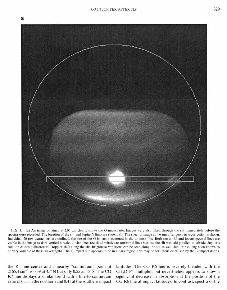
imaging Jupiter through the slit at 2.1 em; the 21-hr-old impact latitude. Observing conditions were good, resultingin high quality data. The CO line in the preimpact spectraG impact site was well situated in the field of view relative

to the slit position. Figure 3a shows an image of Jupiter is essentially identical to the line seen in postimpact spec-tra, both near and well away from the impact sites.at 2.1 em without a slit in place that we recorded after

completing our measurement of the spectra. The spectral Observations on the nights of 1–2 August 1994, 10 daysafter the last impact, covered almost the full range of jovianimage obtained at approximately 5:00 UT is shown in Fig.

3b after correction for geometric distortion. Spectra were longitude at the impact latitudes. On these nights we alsoobserved several other jovian latitudes to provide compari-extracted from this corrected image by coadding groups

of 20 rows (4 arc sec) along the slit (Fig. 4). The 20-row son spectra; frame averaged spectra are shown in Fig. 5.As we have noted previously (Orton et al. 1995), on Augustextraction centered on the G-site is identified in Fig. 4. We

have deleted points within 0.05 cm21 of the center of the 2 the CO R5 line is significantly weaker in the spectraobtained near the impact latitudes. The R6 and R7 linesterrestrial CO line from the ratio and smoothed the spectra

with a 2-point box. are also weaker. The CO line depths are significantly lessthan the same lines on other nights or on the same nightExamination of the individual spectra, including the

spectrum of the G impact site, shows a distinct lack of at comparable northern latitudes. The ratio of intensity at

CO IN JUPITER AFTER SL9 329

FIG. 3. (a) An image obtained at 2.05 em clearly shows the G impact site. Images were also taken through the slit immediately before thespectra were recorded. The location of the slit and Jupiter’s limb are shown. (b) The spectral image at 4.6 em after geometric correction is shown.Individual 20-row extractions are outlined, the site of the G-impact is centered in the topmost box. Both terrestrial and jovian spectral lines arevisible in the image as dark vertical streaks. Jovian lines are tilted relative to terrestrial lines because the slit was laid parallel to latitude. Jupiter’srotation causes a differential Doppler shift along the slit. Brightness variations can be seen along the slit as well. Jupiter has long been known tobe very variable at these wavelengths. The G-impact site appears to be in a dark region; this may be fortuitous or caused by the G-impact debris.

the R5 line center and a nearby ‘‘continuum’’ point at latitudes. The CO R6 line is severely blended with theCH3D P4 multiplet, but nevertheless appears to show a2165.4 cm21 is 0.39 at 458 N but only 0.55 at 458 S. The CO

R7 line displays a similar trend with a line-to-continuum significant decrease in absorption at the position of theCO R6 line at impact latitudes. In contrast, spectra of theratio of 0.53 in the northern and 0.41 at the southern impact

330 NOLL ET AL.

FIG. 3—Continued

CO R7 line on the previous night, August 1 (not shown), lines are observed only in the slit positions near the impactsites. Thus, we must consider the possibility of a real changeshow no difference between the impact latitudes and those

well away from the impact sites. Because the observations in jovian CO lines, discussed in greater detail below.We reobserved the impact sites in March 1995, nearlywere separated by approximately 24 hr, the August 1 data

sample a range of longitudes nearly opposite those sampled 8 months after the impacts. By this time the visible debrishad spread significantly in both longitude and latitude. Ason August 2. The impact latitude spectra were centered

at 1258 for the August 1 R7 line and 2618 and 3098 for the shown in Fig. 5, these spectra look very similar to thosemeasured in July and August 1994. No dramatic changeAugust 2 R7 and R5 line observations, respectively.

The weakening of the CO lines near impact latitudes in in CO line shapes or depths occurred over the 8 monthsfollowing the impacts.Jupiter’s southern hemisphere appears to be a real phe-

nomenon. Some caution must be expressed because ob- By directly comparing the spectra shown in Fig. 5 andothers not shown, we find no evidence for changes in theserving conditions were less than optimal with some cirrus

on both August nights. The spectra display peaks (Fig. 5a) CO lines with the possible exception of August 2. Weconclude that the Comet Shoemaker–Levy 9 impacts didat the positions of terrestrial absorption lines, such as the

N2O line at the Doppler-shifted frequency of 2173.7 cm21. not measurably affect the CO R5 or R7 spectral lines indata taken within hours to 8 months after the impacts.Both stellar and Jupiter spectra were obtained at similar

airmasses and close in time (Jupiter, z 5 1.19; a Vir, z 5 We discuss the implications of this conclusion in moredetail below.1.37 (for the R7 line); Jupiter, z 5 1.33; a Vir, z 5 1.43 (for

the R5 line)). The residual lines in the ratio are indicative ofchanging background levels associated with variable cirrus 5. DISCUSSIONwhich also reduces the S/N obtained on these nights. How-ever, terrestrial CO lines are shifted by 10.19 cm21 relative Carbon monoxide was the most abundant molecule ob-

served after the impacts with a mass for the G impact siteto the jovian CO lines on this night and the weakened CO

CO IN JUPITER AFTER SL9 331

ity of plume material was deposited at low pressures (e.g.,Maillard et al. 1995, Marten et al. 1995, Griffith et al. 1997).

Even large quantities of CO can be hidden from detec-tion at 4.7 em if the CO is present at low pressures. Thisis caused by the dependence of line width on both thermaland pressure-broadening. For temperatures of approxi-mately 200 K the thermally broadened gaussian line shapehas a FWHM of 0.003 cm21. The pressure broadened lo-rentzian component of the line shape has an approximateFWHM 5 P (bars) 3 0.06 cm21. At pressures less than 50mbar the line shape is dominated by the thermal compo-nent, and is very narrow compared to our resolution of0.11 cm21. At low pressure, additional CO results in onlysmall increases in equivalent width since the line quicklyreaches the flat portion of the curve of growth.

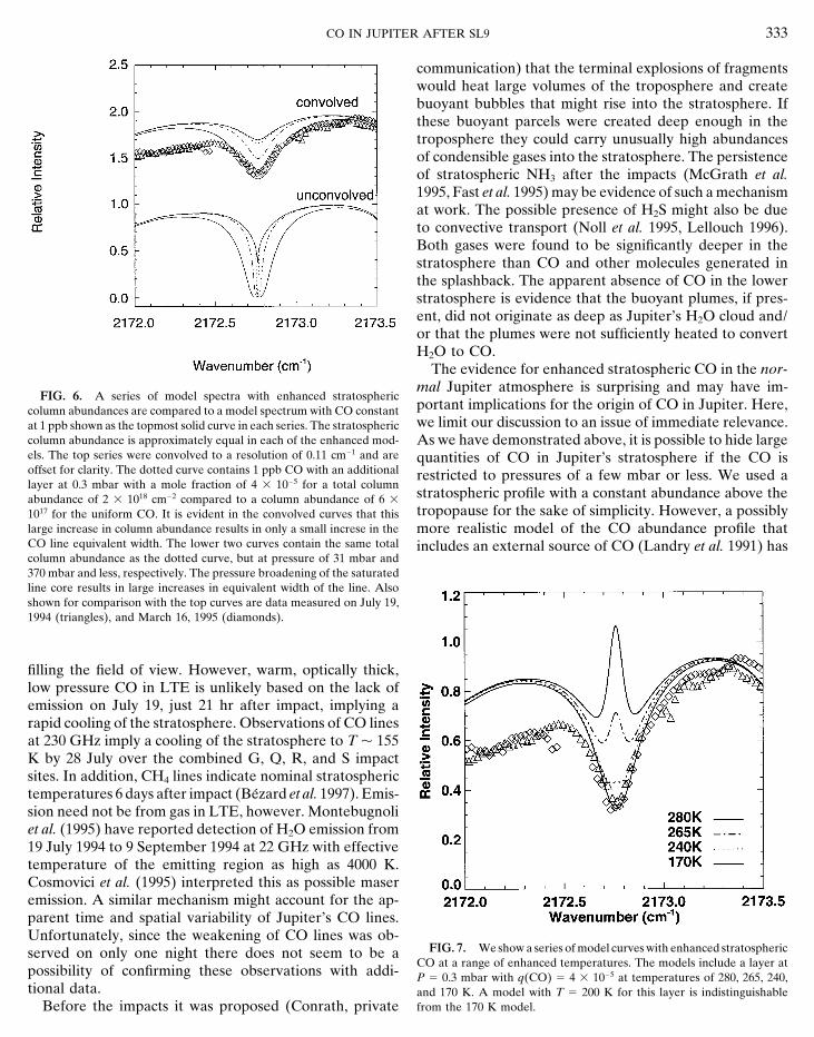
We demonstrate this effect in Fig. 6. The Lellouch et al.CO profile was added to the initially uniform CO profileshown in the topmost curve. The CO column abundance,N 5 6 3 1017 cm22, increased more than 3 times to N 52 3 1018 cm22 by this addition. Despite this, the resultantspectrum shown by the dotted curve in Fig. 6 has an unde-tectably small increase in the depth of the CO line whenconvolved to the spectral resolution of our observations.Examination of the unconvolved model spectra shows why.

FIG. 4. Twenty row (4 arcsec along the slit) summed spectra from The low-pressure CO results in a very high optical depth,19 July with the slit parallel to the impact latitudes. The G-impact site but extremely narrow line core superposed on the muchis centered in row 111. Two 20-row spectra offset by 610 rows are also

broader tropospheric CO line. The two lower curves in theshown. The remaining portion of the slit is shown in steps of 20 rows.figure show the effects of spreading the same stratosphericData have been smoothed with a 2-point box. There are no apparent

strong differences between the spectrum at the 21-hr-old G impact site column abundance to successively higher pressures. Atand other longitudes along the slit. We have masked out a region within P 5 31 mbar the unconvolved line is significantly broader1 resolution element (5 pixels) of the center of the terrestrial CO line. and has begun to develop broad lorentzian wings. At P 5Jupiter’s rotation results in a differential Doppler shift along the slit.

370 mbar the added column abundance results in a linecore with a FWHM comparable to our spectral resolution.The effects of added stratospheric CO are drastically re-duced when we begin with a baseline CO distribution thatalone estimated at 1 3 1014 g (see review by Lellouch

1996). It was observed after the impacts at 230.5 GHz for includes an enhanced stratospheric abundance as seems tobe required by our off-impact and preimpact data (previousmany weeks (Lellouch et al. 1995) and at 2.3 and 4.7 em

in emission immediately after impacts (Ruiz et al. 1995, section). In that case a column abundance of 2 3 1018

cm22 is not detectable regardless of its distribution in theKnacke et al. 1997, Maillard et al. 1995, Brooke et al. 1996).It is reasonable, then, to ask why we do not observe clear stratosphere. Therefore, we conclude that the absence of

observable effects in the CO lines is consistent with evi-changes to CO at 4.7 em days to months after the impacts.The answer is a function of the thermal history and altitude dence from the millimeter-wave spectra that impact-gener-

ated CO did not extend below 0.3 mbar.distribution of the impact-generated CO and other contam-inants. While large column abundances of stratospheric CO can

be essentially invisible at 4.7 em at normal temperatures,The most reliable estimate of postimpact CO abundanceand vertical distribution comes from millimeter wave ob- narrow line cores can become visible in emission when

stratospheric temperatures are elevated. Maillard et al.servations (Lellouch et al. 1995). Analysis of line shapesconstrains both the temperature and vertical distribution (1995) and Brooke et al. (1996) observed emission cores

in multiple lines of the CO 1–0 band approximately 4 hrof CO. Under the assumption that the line widths arecaused by pressure-broadening, Lellouch et al. conclude after the impact of fragment L. Maillard et al. find that a

temperature of T 5 274 K above 0.3 mbar provides athat CO is concentrated above 0.3 mbar. Assuming a tem-perature of 200 K at P , 2 mbar, they find a CO mole good fit to the observed line profile assuming a column

abundance of 1.5 6 0.8 3 1017 cm22. Models with a tempera-fraction of q(CO) 5 4 3 1025. This scenario is consistentwith observations of other molecules that show the major- ture gradient in the stratosphere increasing with altitude

332 NOLL ET AL.

FIG. 5. (a) A sequence of frame-averaged spectra of the CO R7 line from May 1994 through March 1995 are shown as diamonds. Overplottedas solid curves is a model spectrum convolved to the resolution of the observations. The model incorporates CO at 1.3 ppb in the troposphere withan enhanced mole fraction of 100 ppb above the tropopause at pressure levels of 200 mbar and less. (b) A similar sequence for the CO R5 line.Here we also show spectra obtained at similar latitudes in the northern hemisphere, well away from the impacts. There appears to be a weakeningof the CO line on August 2, though it is also apparent that the noise on this night is higher than on other nights. The spectra from August havebeen smoothed with a 2-point box.

give a better match to the column abundance derived by have been undetectable. Our nondetection of emissionlines 21 hr after the G impact is consistent with this cooling.Lellouch et al. (1995). Brooke et al. find very similar results.

When Maillard reobserved the L-impact site approxi- If we make the assumption that the behavior of CO linesin impacts L and G, both large impacts, were similar, andmately 24-hr after impact they did not detect any emission.

Similarly, our observations show no sign of emission in the we use observations of the 1–0 band of CO alone to con-strain the cooling rate, we find that the atmosphere mustCO lines observed on 19 July, approximately 21 hr after

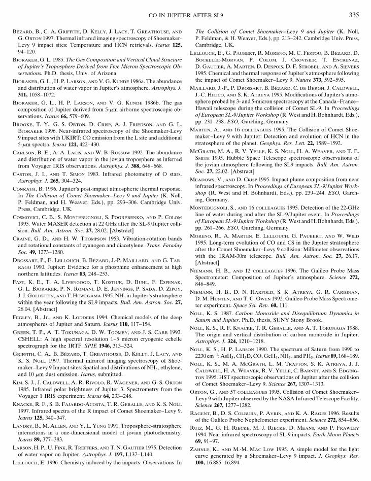
the fragment G impact. have cooled at an average rate of at least 2 K per hour inthe interval between impact 1 4.5 hr and impact 1 21 hr.The series of model spectra shown in Fig. 7 give some

idea of the range of temperatures detectable by us assum- When we use all available observations to constrain thecooling rates for a ‘‘typical’’ large impact site, cooling froming a stratospheric abundance of CO of q(CO) 5 4 3 1025

above 0.3 mbar. The upper two curves with T 5 280 and T 5 274–280 K at impact 1 4.5 hr (Brooke et al. 1996,Maillard et al. 1995) to T 5 200 K at impact 1 10 hr265 K show clear changes in the shape of the spectral line

with distinct emission cores. This line morphology was not (Lellouch et al. 1995, Bezard et al. 1997, Conrath 1996) anaverage cooling rate of at least 11 K hr21 is implied. Theobserved. For stratospheric gas at T 5 240 K the change

in line shape becomes less noticeable, though the line ap- Brooke et al. spectra span a time range from impact 1 3.7hr to impact 1 5.3 hr during which the temperature shouldpears to be significantly weakened. At T # 200 K the

line shape is indistinguishable from the basline model at have decreased by 18 K, a difference that is easily observ-able as shown by the two top curves in Fig. 7. No sucha spectral resolution of 0.1 cm21. Based on a number of

reported observations, it appears that within 10 hr of a change has been reported, but should be sought in existingdata sets.large impact the stratosphere has cooled to T p 200 K at

P p 0.1 mbar (Lellouch et al. 1995, CO lines at 1.3 mm The anomalous results on August 2 can be explained asunresolved emission from CO at low pressure (i.e., a nar-10–14 hr after the G impact; Bezard et al. 1997, CH4 line

at 8.1 em 11 hr after the L impact; Conrath 1996, review row FWHM) partially filling in the broader CO absorptionline core. The observed weakened CO line can be well fitand synthesis). Thus, by 10 hr after a large impact, had

anyone looked, emission lines from CO at 4.7 em would by a model with enhanced stratospheric CO at T p 240 K

CO IN JUPITER AFTER SL9 333

communication) that the terminal explosions of fragmentswould heat large volumes of the troposphere and createbuoyant bubbles that might rise into the stratosphere. Ifthese buoyant parcels were created deep enough in thetroposphere they could carry unusually high abundancesof condensible gases into the stratosphere. The persistenceof stratospheric NH3 after the impacts (McGrath et al.1995, Fast et al. 1995) may be evidence of such a mechanismat work. The possible presence of H2S might also be dueto convective transport (Noll et al. 1995, Lellouch 1996).Both gases were found to be significantly deeper in thestratosphere than CO and other molecules generated inthe splashback. The apparent absence of CO in the lowerstratosphere is evidence that the buoyant plumes, if pres-ent, did not originate as deep as Jupiter’s H2O cloud and/or that the plumes were not sufficiently heated to convertH2O to CO.

The evidence for enhanced stratospheric CO in the nor-mal Jupiter atmosphere is surprising and may have im-

FIG. 6. A series of model spectra with enhanced stratosphericportant implications for the origin of CO in Jupiter. Here,column abundances are compared to a model spectrum with CO constantwe limit our discussion to an issue of immediate relevance.at 1 ppb shown as the topmost solid curve in each series. The stratospheric

column abundance is approximately equal in each of the enhanced mod- As we have demonstrated above, it is possible to hide largeels. The top series were convolved to a resolution of 0.11 cm21 and are quantities of CO in Jupiter’s stratosphere if the CO isoffset for clarity. The dotted curve contains 1 ppb CO with an additional restricted to pressures of a few mbar or less. We used alayer at 0.3 mbar with a mole fraction of 4 3 1025 for a total column

stratospheric profile with a constant abundance above theabundance of 2 3 1018 cm22 compared to a column abundance of 6 3tropopause for the sake of simplicity. However, a possibly1017 for the uniform CO. It is evident in the convolved curves that this

large increase in column abundance results in only a small increse in the more realistic model of the CO abundance profile thatCO line equivalent width. The lower two curves contain the same total includes an external source of CO (Landry et al. 1991) hascolumn abundance as the dotted curve, but at pressure of 31 mbar and370 mbar and less, respectively. The pressure broadening of the saturatedline core results in large increases in equivalent width of the line. Alsoshown for comparison with the top curves are data measured on July 19,1994 (triangles), and March 16, 1995 (diamonds).

filling the field of view. However, warm, optically thick,low pressure CO in LTE is unlikely based on the lack ofemission on July 19, just 21 hr after impact, implying arapid cooling of the stratosphere. Observations of CO linesat 230 GHz imply a cooling of the stratosphere to T p 155K by 28 July over the combined G, Q, R, and S impactsites. In addition, CH4 lines indicate nominal stratospherictemperatures 6 days after impact (Bezard et al. 1997). Emis-sion need not be from gas in LTE, however. Montebugnoliet al. (1995) have reported detection of H2O emission from19 July 1994 to 9 September 1994 at 22 GHz with effectivetemperature of the emitting region as high as 4000 K.Cosmovici et al. (1995) interpreted this as possible maseremission. A similar mechanism might account for the ap-parent time and spatial variability of Jupiter’s CO lines.Unfortunately, since the weakening of CO lines was ob-

FIG. 7. We show a series of model curves with enhanced stratosphericserved on only one night there does not seem to be aCO at a range of enhanced temperatures. The models include a layer at

possibility of confirming these observations with addi- P 5 0.3 mbar with q(CO) 5 4 3 1025 at temperatures of 280, 265, 240,tional data. and 170 K. A model with T 5 200 K for this layer is indistinguishable

from the 170 K model.Before the impacts it was proposed (Conrath, private

334 NOLL ET AL.

a CO mole fraction that increases with decreasing pressure 20–30 ppm (Fegley and Lodders 1994) and to be wellmixed throughout the atmosphere. Such a large abundanceso that the mole fraction at 1 mbar is up to 300 times

greater than at 100 mbar, reaching 300 ppb for deep atmo- of N2 would mask CO at the 0.1 ppm level or less. On theother hand, an increase in the mass 28 peak at the lowestsphere CO abundances of 1 ppb. Thus it might be possible

to have large mole fractions of CO at pressures of 1 mbar pressure levels sampled by the GPMS might result if astrong enhancement of CO in the stratosphere and upperand less, the pressure levels where the greatest post-SL9

heating occurred (though mole fractions as high as 40 ppm troposphere exists and N2 is less abundant than the maxi-mum predicted.at 0.3 mbar (Lellouch et al. 1995) would not be predicted

by these models).6. CONCLUSIONSKnacke et al. (1997) find that the peak CO 2–0 band head

emission from the R-impact site requires a CO column ofA search for impact-related changes to CO lines in theN(CO) P 4 3 1014 cm22 for T 5 2500 K. Maillard et al.

1–0 rotation–vibration band near 4.7 em yielded negative(1995) and Brooke et al. (1996) find column abundancesresults. We observed the G-impact site 21 hr after theof order N(CO) P 1017 at the L-impact site and Lellouchimpact and continued to observe the impact latitudeet al. (1995, 1996) find N(CO) P 4 3 1018 at the K-impactthrough March 1995. The impacts did not deliver detect-site. It is worth noting that the CO lines observed at milli-able quantities of CO-rich gas to the upper troposphere/meter wavelengths appeared first as emission lines andlower stratosphere region of the atmosphere probed atlater as absorption lines (Lellouch et al. 1995). Thus, therethese wavelengths. One possible exception occurred on 2exists at least one thermal profile where this column abun-August 1994 when we detected weakened CO lines neardance of CO is not detectable at millimeter wavelengthsimpact latitudes but ‘‘normal’’ lines well away from the(though apparently this is cooler than the normal strato-impacts. If the line were filled in by an unresolved emissionspheric thermal profile; Lellouch et al. 1995). In an un-core, the excitation mechanism must be nonthermal to beheated stratosphere, we have shown that any of these COconsistent with the lack of CO emission 21 hr after the Gcolumn abundances are undetectable at 4.7 em if the COimpact and other observations that show the stratosphereis at low pressures. Thus, some caution may be needed incooled quickly after the impacts.identifying CO as cometary debris, particularly for the

We could not fit the observed pre- or postimpact lineobservations of the CO 2–0 and other bandheads at 2.3shapes with a simple constant-abundance CO profile inem. Because CO is thought to be the main product ofcontradiction to earlier published results (Noll et al. 1988).shock chemistry on the cometary material, the mass of COThe reason for this difference requires further investiga-derived by Lellouch et al. (1995, 1996) has been used totion, but may be related to the lower sensitivity of earlierestimate the mass of the fragments which were approxi-observations. We found a fit with a simple two-value abun-mately half oxygen by mass. A large preexisting abundancedance profile that includes a significant enhancement ofof CO in the upper stratosphere could complicate thisCO in the stratosphere. Some of the CO detected afterapproach. If a profile similar to the CO profile proposedthe SL9 impacts may simply be preexisting jovian COby Landry et al. (1991) exists in Jupiter, several percent ofheated by the plume splashback. If so, caution may bethe CO observed at 1.3 mm and all of the CO observedrequired in estimating the mass of the fragments fromat 2.3 em could have been present in Jupiter before thededuced CO masses, particularly from observations of theSL9 impacts.CO 2–0 and higher bandheads.The Galileo Mass Spectrometer experiment (GPMS)

The Galileo Probe Mass Spectrometer experiment maysampled Jupiter’s troposphere and detected a prominentbe able to detect an enhanced abundance of jovian CO inpeak at mass 28 in the two sample mass spectra shown bythe upper troposphere in the peak at mass 28, but may beNiemann et al. (1996). The peak is identified only as two-confused with potentially more-abundant N2 .carbon hydrocarbons, presumably ethylene, C2H4 , at mass

28.03130 amu. However, ethylene has been detected onlyACKNOWLEDGMENTSin the stratosphere near the north polar hood with a mole

fraction of 7 ppb (Kim et al. 1985) which is below the lower This research was supported by Grants NAGW-3392 to the Spacelimit for detection of p50 ppb with the GPMS. Both 12C16O Telescope Science Institute and NAGW-3415 and NAGW-4124 to the

Pennsylvania State University, Erie, from the NASA Research in Plane-and 14N2 can also contribute to this peak with masses oftary Astronomy program.27.99491 and 28.00615 amu, respectively. The highest mass-

resolution possible with the GPMS is 0.125 amu (NiemannREFERENCESet al. 1992); therefore the signals of CO, N2 , and C2H4 are

blended, though analysis of lower mass fragments can, in ANDERS, E., AND N. GREVESSE 1989. Abundances of the elements: Mete-principle, allow identification of the individual compo- oritic and solar. Geochim. Cosmochim. Acta 53, 197–214.nents. N2 has not been detected in Jupiter’s atmosphere BEER, R. 1975. Detection of carbon monoxide in Jupiter. Astrophys. J.

200, L167–L169.but is predicted to be present in abundances as high as

CO IN JUPITER AFTER SL9 335

BEZARD, B., C. A. GRIFFITH, D. KELLY, J. LACY, T. GREATHOUSE, AND The Collision of Comet Shoemaker–Levy 9 and Jupiter (K. Noll,P. Feldman, & H. Weaver, Eds.), pp. 213–242. Cambridge Univ. Press,G. ORTON 1997. Thermal infrared imaging spectroscopy of Shoemaker-

Levy 9 impact sites: Temperature and HCN retrievals. Icarus 125, Cambridge, UK.94–120. LELLOUCH, E., G. PAUBERT, R. MORENO, M. C. FESTOU, B. BEZARD, D.

BOCKELEE-MORVAN, P. COLOM, J. CROVISIER, T. ENCRENAZ,BJORAKER, G. L. 1985. The Gas Composition and Vertical Cloud Structureof Jupiter’s Troposphere Derived from Five Micron Spectroscopic Ob- D. GAUTIER, A. MARTEN, D. DESPOIS, D. F. STROBEL, AND A. SIEVERS

1995. Chemical and thermal response of Jupiter’s atmosphere followingservations. Ph.D. thesis, Univ. of Arizona.the impact of Comet Shoemaker–Levy 9. Nature 373, 592–595.BJORAKER, G. L., H. P. LARSON, AND V. G. KUNDE 1986a. The abundance

and distribution of water vapor in Jupiter’s atmosphere. Astrophys. J. MAILLARD, J.-P., P. DROSSART, B. BEZARD, C. DE BERGH, J. CALDWELL,J.-C. HILICO, AND S. K. ATREYA 1995. Modifications of Jupiter’s atmo-311, 1058–1072.sphere probed by 3- and 5-micron spectroscopy at the Canada–France–BJORAKER, G. L., H. P. LARSON, AND V. G. KUNDE 1986b. The gasHawaii telescope during the collision of Comet SL-9. In Proceedingscomposition of Jupiter derived from 5-em airborne spectroscopic ob-of European SL-9/Jupiter Workshop (R. West and H. Bohnhardt, Eds.),servations. Icarus 66, 579–609.pp. 231–238. ESO, Garching, Germany.BROOKE, T. Y., G. S. ORTON, D. CRISP, A. J. FRIEDSON, AND G. L.

MARTEN, A., AND 16 COLLEAGUES 1995. The Collision of Comet Shoe-BJORAKER 1996. Near-infrared spectroscopy of the Shoemaker-Levymaker–Levy 9 with Jupiter: Detection and evolution of HCN in the9 impact sites with UKIRT: CO emission from the L site and additionalstratosphere of the planet. Geophys. Res. Lett. 22, 1589–1592.5-em spectra. Icarus 121, 422–430.

MCGRATH, M. A., R. V. YELLE, K. S. NOLL, H. A. WEAVER, AND T. E.CARLSON, B. E., A. A. LACIS, AND W. B. ROSSOW 1992. The abundanceSMITH 1995. Hubble Space Telescope spectroscopic observations ofand distribution of water vapor in the jovian troposphere as inferredthe jovian atmosphere following the SL9 impacts. Bull. Am. Astron.from Voyager IRIS observations. Astrophys. J. 388, 648–668.Soc. 27, 22.02. [Abstract]CASTOR, J. I., AND T. SIMON 1983. Infrared photometry of O stars.

MEADOWS, V., AND D. CRISP 1995. Impact plume composition from nearAstrophys. J. 265, 304–324.infrared spectroscopy. In Proceedings of European SL-9/Jupiter Work-CONRATH, B. 1996. Jupiter’s post-impact atmospheric thermal response.shop (R. West and H. Bohnhardt, Eds.), pp. 239–244. ESO, Garch-In The Collision of Comet Shoemaker–Levy 9 and Jupiter (K. Noll,ing, Germany.P. Feldman, and H. Weaver, Eds.), pp. 293–306. Cambridge Univ.

MONTEBUGNOLI, S., AND 16 COLLEAGUES 1995. Detection of the 22-GHzPress, Cambridge, UK.line of water during and after the SL-9/Jupiter event. In ProceedingsCOSMOVICI, C. B., S. MONTEBUGNOLI, S. POGREBENKO, AND P. COLOMof European SL-9/Jupiter Workshop (R. West and H. Bohnhardt, Eds.),1995. Water MASER detection at 22 GHz after the SL-9/Jupiter colli-pp. 261–266. ESO, Garching, Germany.sion. Bull. Am. Astron. Soc. 27, 28.02. [Abstract]

MORENO, R., A. MARTEN, E. LELLOUCH, G. PAUBERT, AND W. WILDCRAINE, G. D., AND H. W. THOMPSON 1953. Vibration-rotation bands1995. Long-term evolution of CO and CS in the Jupiter stratosphereand rotational constants of cyanogen and diacetylene. Trans. Faradayafter the Comet Shoemaker–Levy 9 collision: Millimeter observationsSoc. 49, 1273–1280.with the IRAM-30m telescope. Bull. Am. Astron. Soc. 27, 26.17.

DROSSART, P., E. LELLOUCH, B. BEZARD, J.-P. MAILLARD, AND G. TAR- [Abstract]RAGO 1990. Jupiter: Evidence for a phosphine enhancement at high

NIEMANN, H. B., AND 12 COLLEAGUES 1996. The Galileo Probe Massnorthern latitudes. Icarus 83, 248–253.

Spectrometer: Composition of Jupiter’s atmosphere. Science 272,FAST, K. E., T. A. LIVENGOOD, T. KOSTIUK, D. BUHL, F. ESPENAK, 846–849.

G. L. BJORAKER, P. N. ROMANI, D. E. JENNINGS, P. SADA, D. ZIPOY,NIEMANN, H. B., D. N. HARPOLD, S. K. ATREYA, G. R. CARIGNAN,

J. J. GOLDSTEIN, AND T. HEWEGAMA 1995. NH3 in Jupiter’s stratosphere D. M. HUNTEN, AND T. C. OWEN 1992. Galileo Probe Mass Spectrome-within the year following the SL9 impacts. Bull. Am. Astron. Soc. 27, ter experiment. Space Sci. Rev. 60, 111.26.04. [Abstract]

NOLL, K. S. 1987. Carbon Monoxide and Disequilibrium Dynamics inFEGLEY, B., Jr., AND K. LODDERS 1994. Chemical models of the deep Saturn and Jupiter. Ph.D. thesis, SUNY Stony Brook.

atmospheres of Jupiter and Saturn. Icarus 110, 117–154.NOLL, K. S., R. F. KNACKE, T. R. GEBALLE, AND A. T. TOKUNAGA 1988.

GREEN, T. P., A. T. TOKUNAGA, D. W. TOOMEY, AND J. S. CARR 1993. The origin and vertical distribution of carbon monoxide in Jupiter.CSHELL: A high spectral resolution 1–5 micron cryogenic echelle Astrophys. J. 324, 1210–1218.spectrograph for the IRTF. SPIE 1946, 313–324.

NOLL, K. S., H. P. LARSON 1990. The spectrum of Saturn from 1990 toGRIFFITH, C. A., B. BEZARD, T. GREATHOUSE, D. KELLY, J. LACY, AND 2230 cm21: AsH3 , CH3D, CO, GeH4 , NH3 , and PH3 . Icarus 89, 168–189.

K. S. NOLL 1997. Thermal infrared imaging spectroscopy of Shoe-NOLL, K. S., M. A. MCGRATH, L. M. TRAFTON, S. K. ATREYA, J. J.

maker–Levy 9 Impact sites: Spatial and distributions of NH3 , ethylene, CALDWELL, H. A. WEAVER, R. V. YELLE, C. BARNET, AND S. EDGING-and 10 em dust emission. Icarus, submitted.

TON 1995. HST spectroscopic observations of Jupiter after the collisionKIM, S. J., J. CALDWELL, A. R. RIVOLO, R. WAGENER, AND G. S. ORTON of Comet Shoemaker–Levy 9. Science 267, 1307–1313.

1985. Infrared polar brightness of Jupiter 3. Spectrometry from the ORTON, G., AND 57 COLLEAGUES 1995. Collision of Comet Shoemaker–Voyager 1 IRIS experiment. Icarus 64, 233–248. Levy 9 with Jupiter observed by the NASA Infrared Telescope Facility.

KNACKE, R. F., S. B. FAJARDO-ACOSTA, T. R. GEBALLE, AND K. S. NOLL Science 267, 1277–1282.1997. Infrared spectra of the R impact of Comet Shoemaker–Levy 9. RAGENT, B., D. S. COLBURN, P. AVRIN, AND K. A. RAGES 1996. ResultsIcarus 125, 340–347. of the Galileo Probe Nephelometer experiment. Science 272, 854–856.

LANDRY, B., M. ALLEN, AND Y. L. YUNG 1991. Troposphere-stratosphere RUIZ, M., G. H. RIECKE, M. J. RIECKE, D. MEANS, AND P. FRAWLEYinteractions in a one-dimensional model of jovian photochemistry. 1994. Near infrared spectroscopy of SL-9 impacts. Earth Moon PlanetsIcarus 89, 377–383. 69, 91–97.

LARSON, H. P., U. FINK, R. TREFFERS, AND T. N. GAUTIER 1975. Detection ZAHNLE, K., AND M.-M. MAC LOW 1995. A simple model for the lightof water vapor on Jupiter. Astrophys. J. 197, L137–L140. curve generated by a Shoemaker–Levy 9 impact. J. Geophys. Res.

100, 16,885–16,894.LELLOUCH, E. 1996. Chemistry induced by the impacts: Observations. In