Embed Size (px)
Citation preview
©Prof. Roger G. Mark, 2004
MASSACHUSETTS INSTITUTE OF TECHNOLOGY
Departments of Electrical Engineering, Mechanical Engineering,and the Harvard-MIT Division of Health Sciences and Technology
6.022J/2.792J/HST542J: Quantitative Physiology: Organ Transport Systems
PRINCIPLES OF CARDIAC ELECTROPHYSIOLOGY
I. Electrophysiology of Myocardial CellsII. The Physical Basis of Electrocardiography
Text Reference: pages 115-126
Harvard-MIT Division of Health Sciences and Technology HST.542J: Quantitative Physiology: Organ Transport Systems Instructor: Roger Mark
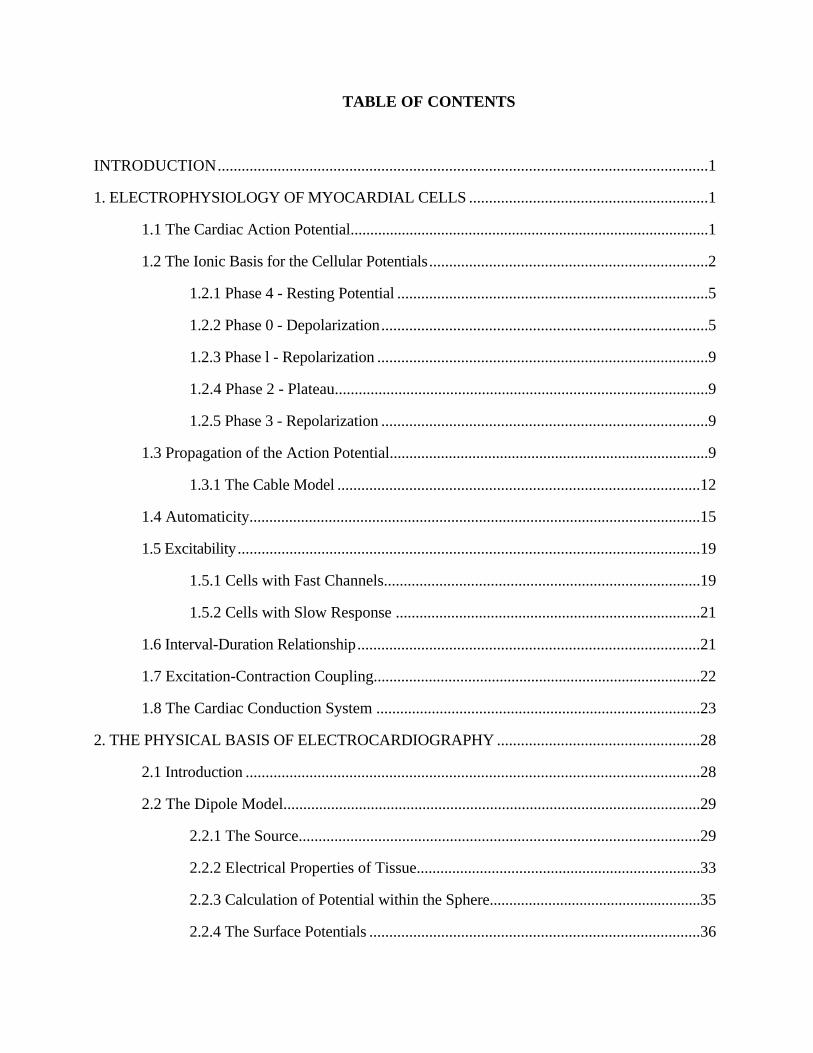
TABLE OF CONTENTS
INTRODUCTION........................................................................................................................... 1
1. ELECTROPHYSIOLOGY OF MYOCARDIAL CELLS............................................................ 1
1.1 The Cardiac Action Potential........................................................................................... 1
1.2 The Ionic Basis for the Cellular Potentials...................................................................... 2
1.2.1 Phase 4 - Resting Potential.............................................................................. 5
1.2.2 Phase 0 - Depolarization.................................................................................. 5
1.2.3 Phase l - Repolarization................................................................................... 9
1.2.4 Phase 2 - Plateau.............................................................................................. 9
1.2.5 Phase 3 - Repolarization.................................................................................. 9
1.3 Propagation of the Action Potential................................................................................. 9
1.3.1 The Cable Model........................................................................................... 12
1.4 Automaticity.................................................................................................................. 15
1.5 Excitability.................................................................................................................... 19
1.5.1 Cells with Fast Channels................................................................................ 19
1.5.2 Cells with Slow Response ............................................................................. 21
1.6 Interval-Duration Relationship...................................................................................... 21
1.7 Excitation-Contraction Coupling................................................................................... 22
1.8 The Cardiac Conduction System .................................................................................. 23
2. THE PHYSICAL BASIS OF ELECTROCARDIOGRAPHY................................................... 28
2.1 Introduction.................................................................................................................. 28
2.2 The Dipole Model......................................................................................................... 29
2.2.1 The Source..................................................................................................... 29
2.2.2 Electrical Properties of Tissue........................................................................ 33
2.2.3 Calculation of Potential within the Sphere...................................................... 35
2.2.4 The Surface Potentials................................................................................... 36
2.3 Lead Systems Used in Scalar Electrocardiography....................................................... 39
2.3.1 Frontal Plane Scalar Leads............................................................................. 40
2.3.2 Precordial Leads............................................................................................ 42
2.4 Electrical Axis............................................................................................................... 44
Principles of Cardiac Electrophysiology 1
PRINCIPLES OF CARDIAC ELECTROPHYSIOLOGY
INTRODUCTlON
The heart’s pumping action depends on the rhythmic, coordinated contraction of the
ventricles and the proper functioning of the valves. Each mechanical heartbeat is triggered by an
action potential which originates from a rhythmic, pacemaker cell within the heart. The impulse is
then conducted rapidly throughout the organ in order to produce coordinated contraction.
Disturbances in the heart’s electrical activity may cause significant abnormalities in its mechanical
function, and are the basis of much cardiac morbidity and mortality. In fact, malfunction of the
heart’s electrical behavior is the principal cause of sudden cardiac death. This chapter will discuss
cardiac electrophysiology beginning at the cellular level. We will then explore the anatomy and
electrophysiology of the cardiac conduction system, and the normal sequence of myocardial
depolarization. Finally, we will relate the electrical activity of the myocardium to body surface
potentials using the simple dipole model.
ELECTROPHYSIOLOGY OF MYOCARDIAL CELLS
1.1 The Cardiac Action Potential
Cardiac transmembrane potentials may be recorded by means of microelectrodes. A typical
resting potential in a ventricular muscle fiber is -80 to-90 millivolts with respect to surrounding
extracellular fluid, similar to that found in nerve and skeletal muscle. The shape of the cardiac action
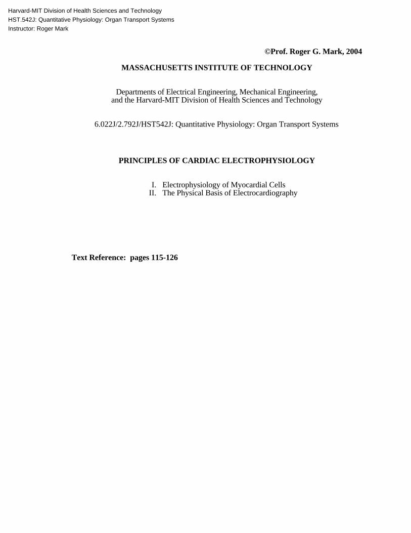
potential, however, is quite distinctive primarily because of its long duration. A typical action
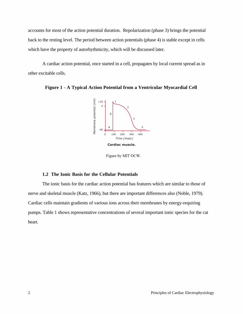
potential from a ventricular cell is diagrammed in Fig. 1. Its total duration may be 200-300
milliseconds (in contrast to 1 or 2 milliseconds for nerve and skeletal muscle), and it consists of 5
distinct phases. The initial rapid upstroke (phase 0) from the resting potential to a positive value of
about +20 millivolts is similar to the spikes of other cells. Early repolarization (phase 1) brings the
potential down to a plateau level over 2 to 3 milliseconds. The plateau itself (phase 2) follows, and
2 Principles of Cardiac Electrophysiology
accounts for most of the action potential duration. Repolarization (phase 3) brings the potential
back to the resting level. The period between action potentials (phase 4) is stable except in cells
which have the property of autorhythmicity, which will be discussed later.
A cardiac action potential, once started in a cell, propagates by local current spread as in
other excitable cells.
Figure 1 - A Typical Action Potential from a Ventricular Myocardial Cell
1.2 The Ionic Basis for the Cellular Potentials
The ionic basis for the cardiac action potential has features which are similar to those of
nerve and skeletal muscle (Katz, 1966), but there are important differences also (Noble, 1979).
Cardiac cells maintain gradients of various ions across their membranes by energy-requiring
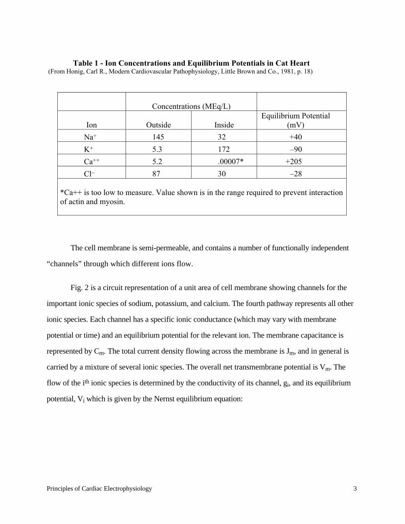
pumps. Table 1 shows representative concentrations of several important ionic species for the cat
heart.
+20
0
-90
0
Time (msec)
Mem
bra
ne
pote
ntial
(m
V)
100 200 300 400
Cardiac muscle.
1
0
2
3
44
Figure by MIT OCW.
Principles of Cardiac Electrophysiology 3
The cell membrane is semi-permeable, and contains a number of functionally independent
“channels” through which different ions flow.
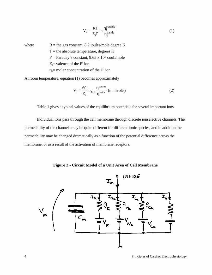
Fig. 2 is a circuit representation of a unit area of cell membrane showing channels for the
important ionic species of sodium, potassium, and calcium. The fourth pathway represents all other
ionic species. Each channel has a specific ionic conductance (which may vary with membrane
potential or time) and an equilibrium potential for the relevant ion. The membrane capacitance is
represented by Cm. The total current density flowing across the membrane is Jm, and in general is
carried by a mixture of several ionic species. The overall net transmembrane potential is Vm. The
flow of the ith ionic species is determined by the conductivity of its channel, gi, and its equilibrium
potential, Vi which is given by the Nernst equilibrium equation:
Table 1 - Ion Concentrations and Equilibrium Potentials in Cat Heart (From Honig, Carl R., Modern Cardiovascular Pathophysiology, Little Brown and Co., 1981, p. 18)
Concentrations (MEq/L)
Ion
Outside
Inside
Equilibrium Potential (mV)
Na+ 145 32 +40 K+ 5.3 172 –90 Ca++ 5.2 .00007* +205 Cl– 87 30 –28
*Ca++ is too low to measure. Value shown is in the range required to prevent interaction of actin and myosin.
4 Principles of Cardiac Electrophysiology
V i = RTZ iF
lnηi
outside
ηiinside (1)
where R = the gas constant, 8.2 joules/mole degree K
T = the absolute temperature, degrees K
F = Faraday’s constant, 9.65 x 10⁴ coul./mole
Zi= valence of the ith ion
ηi= molar concentration of the ith ion
At room temperature, equation (1) becomes approximately
V i = 60Z i
log10
ηioutside
ηiinside (millivolts) (2)
Table 1 gives a typical values of the equilibrium potentials for several important ions.
Individual ions pass through the cell membrane through discrete ionselective channels. The
permeability of the channels may be quite different for different ionic species, and in addition the
permeability may be changed dramatically as a function of the potential difference across the
membrane, or as a result of the activation of membrane receptors.
Figure 2 - Circuit Model of a Unit Area of Cell Membrane
Principles of Cardiac Electrophysiology 5
From the circuit of Fig. 2 we have the following expression for the membrane current
density Jm:
Jm = Cm
dVmdt
+ gi V m − V i( )i
∑ (3)
where Cm is the membrane capacitance, Vm is the transmembrane potential, and gi is the membrane
conductance for the ionic species, i.
Phase 4 - Resting Potential
The resting potential (phase 4) in non-pacemaker cardiac cells is established by the same
mechanisms as for other excitable cells. Referring to the model during the resting state
(dVm/dt = 0), and assuming no externally applied current, we have Jm = 0. Solving eq. (3) for the
resultant potential, we have
V m0 = gK
gm
VK + gNa
gm
V Na + gCa
gm
VCa + g0
gm
V 0 (4)
where
gm = gii
∑
and V m0 is the resting potential. In the resting state the cell membrane is much more permeable to
potassium than to the other ions, hence gK/gm ≈1. As a result, the resting potential is close to VK:
typically –80 to –90 mV in ventricular myocardial cells.
1.2.2 Phase 0 — Depolarization
The ionic mechanism underlying phase 0 depolarization in most cardiac muscle cells is
similar to that of nerve and skeletal muscle—namely a rapid (and transient) regenerative increase in
6 Principles of Cardiac Electrophysiology
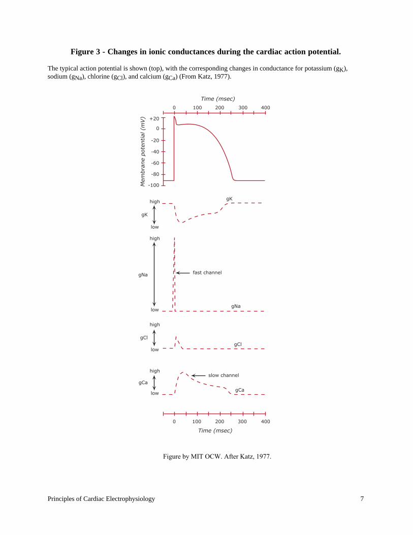
sodium conductance, gNa to values almost two orders of magnitude greater than peak gK or gCa.
This permits the membrane potential to shift toward the sodium equilibrium potential (+40 mV).
The fact that the action potential never reaches VNa reflects the residual permeability of the
membrane to potassium. It has been shown that phase 0 is also accompanied by a fall in potassium
conductance, with much slower kinetics. (See Fig. 3.)
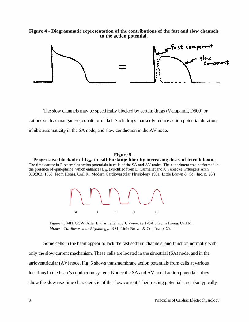
It has been demonstrated that there is a second important inward (depolarizing) current
which is activated by depolarization of the cell. This current is not sensitive to variations in
extracellular sodium concentration, but is very sensitive to extracellular calcium concentration. The
kinetics of this second current are very sluggish, both during activation and inactivation. This so-
called “slow inward current” is carried primarily by calcium ions and plays an important role in the
activation of mechanical contraction. Most cardiac cells utilize both fast and slow currents. Fig. 4
presents a hypothetical representation of the fast (Na+) and slow (Ca++) components of the
cardiac action potential. (Notice that the slow inward current is the primary determinant of the phase
2 plateau.)
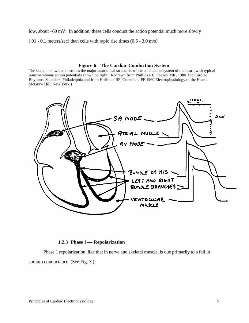
It is possible to selectively disable one or the other of the two inward channels. The sodium
channel may be inactivated by partially depolarizing the membrane to about -60 mV. This channel
may also be selectively blocked by tetrodotoxin (TTX), a poison derived from the Japanese puffer
fish. With the sodium channel blocked, cells will exhibit the slow response only, although
sympathomimetic amines such as epinephrine or isoproternol may be required to stimulate the slow
channel sufficiently to generate action potentials. Fig. 5 shows action potentials of the “slow
response” type in Purkinje cells whose sodium channels were inactivated by increasing doses of
tetrodotoxin (in the presence of epinephrine).
Principles of Cardiac Electrophysiology 7
Figure 3 - Changes in ionic conductances during the cardiac action potential.
The typical action potential is shown (top), with the corresponding changes in conductance for potassium (gK),sodium (gNa), chlorine (gCl), and calcium (gCa) (From Katz, 1977).
+20
0 100
high
high
fast channel
high
high
low
low
low
low
200 300 400
0 100 200 300 400
-20
-40
-60
-80
-100
gK
gNa
gNa
gClgCl
gCa
gCa
gK
0
Time (msec)
Time (msec)
Mem
bra
ne
pote
ntial
(m
V)
slow channel
Figure by MIT OCW. After Katz, 1977.
8 Principles of Cardiac Electrophysiology
Figure 4 - Diagrammatic representation of the contributions of the fast and slow channelsto the action potential.
The slow channels may be specifically blocked by certain drugs (Verapamil, D600) or
cations such as manganese, cobalt, or nickel. Such drugs markedly reduce action potential duration,
inhibit automaticity in the SA node, and slow conduction in the AV node.
Figure 5 -Progressive blockade of INa+ in calf Purkinje fiber by increasing doses of tetrodotoxin.
The time course in E resembles action potentials in cells of the SA and AV nodes. The experiment was performed inthe presence of epinephrine, which enhances Lsi. (Modified from E. Carmeliet and J. Vereecke, Pfluegers Arch.313:303, 1969. From Honig, Carl R., Modern Cardiovascular Physiology 1981, Little Brown & Co., Inc. p. 26.)
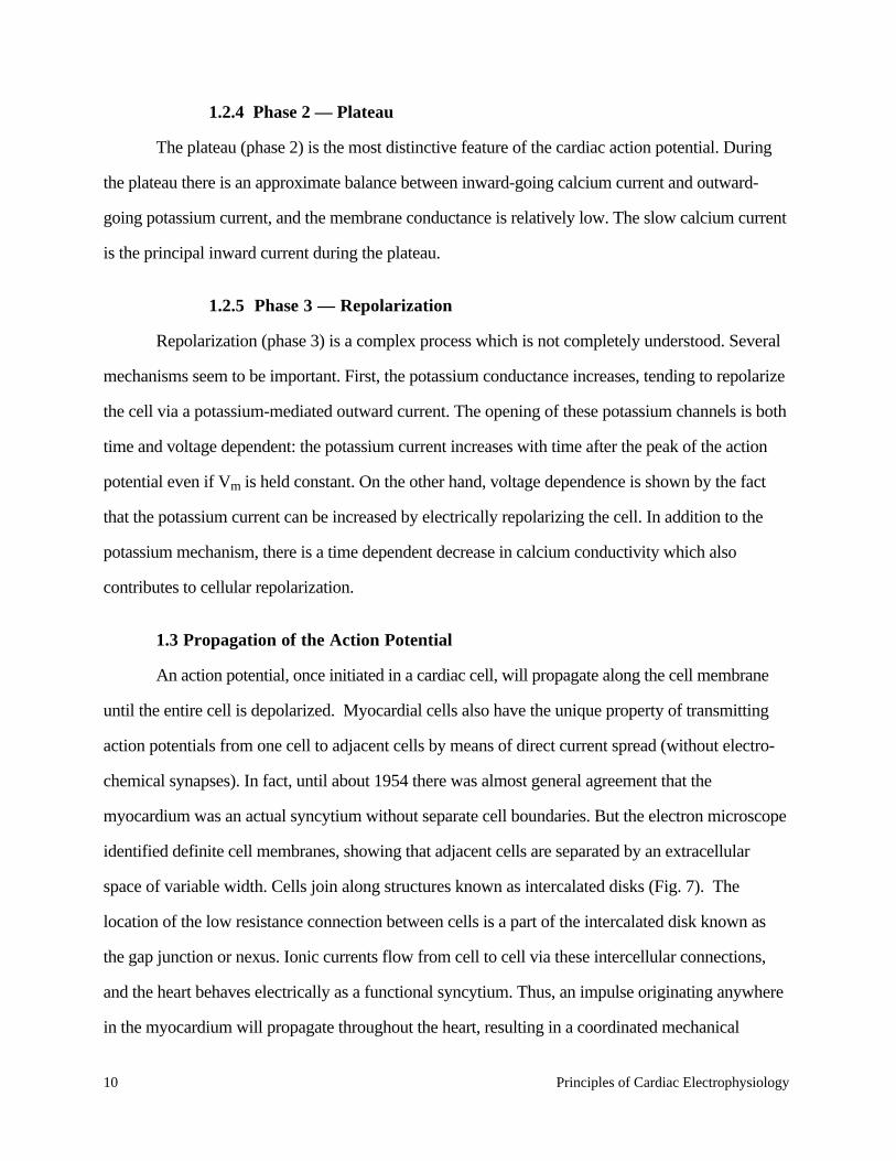
Some cells in the heart appear to lack the fast sodium channels, and function normally with
only the slow current mechanism. These cells are located in the sinoatrial (SA) node, and in the
atrioventricular (AV) node. Fig. 6 shows transmembrane action potentials from cells at various
locations in the heart’s conduction system. Notice the SA and AV nodal action potentials: they
show the slow rise-time characteristic of the slow current. Their resting potentials are also typically
A B C D E
Figure by MIT OCW. After E. Carmeliet and J. Vereecke 1969, cited in Honig, Carl R. Modern Cardiovascular Physiology. 1981, Little Brown & Co., Inc. p. 26.
Principles of Cardiac Electrophysiology 9
low, about –60 mV. In addition, these cells conduct the action potential much more slowly
(.01 - 0.1 meters/sec) than cells with rapid rise times (0.5 - 3.0 m/s).
Figure 6 - The Cardiac Conduction SystemThe sketch below demonstrates the major anatomical structures of the conduction system of the heart, with typicaltransmembrane action potentials shown on right. (Redrawn from Phillips RE, Feeney MK, 1980 The CardiacRhythms. Saunders, Philadelphia and from Hoffman BF, Cranefield PF 1960 Electrophysiology of the Heart.McGraw Hill, New York.)
1.2.3 Phase l — Repolarization
Phase 1 repolarization, like that in nerve and skeletal muscle, is due primarily to a fall in
sodium conductance. (See Fig. 3.)
10 Principles of Cardiac Electrophysiology
1.2.4 Phase 2 — Plateau
The plateau (phase 2) is the most distinctive feature of the cardiac action potential. During
the plateau there is an approximate balance between inward-going calcium current and outward-
going potassium current, and the membrane conductance is relatively low. The slow calcium current
is the principal inward current during the plateau.
1.2.5 Phase 3 — Repolarization
Repolarization (phase 3) is a complex process which is not completely understood. Several
mechanisms seem to be important. First, the potassium conductance increases, tending to repolarize
the cell via a potassium-mediated outward current. The opening of these potassium channels is both
time and voltage dependent: the potassium current increases with time after the peak of the action
potential even if Vm is held constant. On the other hand, voltage dependence is shown by the fact
that the potassium current can be increased by electrically repolarizing the cell. In addition to the
potassium mechanism, there is a time dependent decrease in calcium conductivity which also
contributes to cellular repolarization.
1.3 Propagation of the Action Potential
An action potential, once initiated in a cardiac cell, will propagate along the cell membrane
until the entire cell is depolarized. Myocardial cells also have the unique property of transmitting
action potentials from one cell to adjacent cells by means of direct current spread (without electro-
chemical synapses). In fact, until about 1954 there was almost general agreement that the
myocardium was an actual syncytium without separate cell boundaries. But the electron microscope
identified definite cell membranes, showing that adjacent cells are separated by an extracellular
space of variable width. Cells join along structures known as intercalated disks (Fig. 7). The
location of the low resistance connection between cells is a part of the intercalated disk known as
the gap junction or nexus. Ionic currents flow from cell to cell via these intercellular connections,
and the heart behaves electrically as a functional syncytium. Thus, an impulse originating anywhere
in the myocardium will propagate throughout the heart, resulting in a coordinated mechanical
Principles of Cardiac Electrophysiology 11
contraction. (The atria, however, are electrically insulated from the ventricles except for the AV
node.) An artificial cardiac pacemaker, for example, introduces depolarizing electrical impulses via
an electrode catheter usually placed within the right ventricle. Pacemaker-induced action potentials
excite the entire ventricular myocardium resulting in effective mechanical contractions.
Figure 7 - The Intercalated Disk
Electron microphotographs of the intercalated disc. Top: Transverse section of cat ventricular myocardium, showinginsertions of thin filaments into filamentous mats (arrows), which bind to the intercalated disc to form the fasciaadherens (FA). This intracellular junction changes form at the right of the figure, where the two cells come intocontact at a nexus, of gap junction (N). Bottom: Oblique section of intercalated disc in mouse ventricularmyocardium, showing filaments (arrow) joining fascia adherens (FA) and a nexus (N). Two maculae adherens (MA),or desmosomes, are also shown. All of these structures represent specialized cell-cell junctions. (From McNutt andFawcett (1974), courtesy of Wiley, New York.)
Image removed due to copyright considerations.
12 Principles of Cardiac Electrophysiology
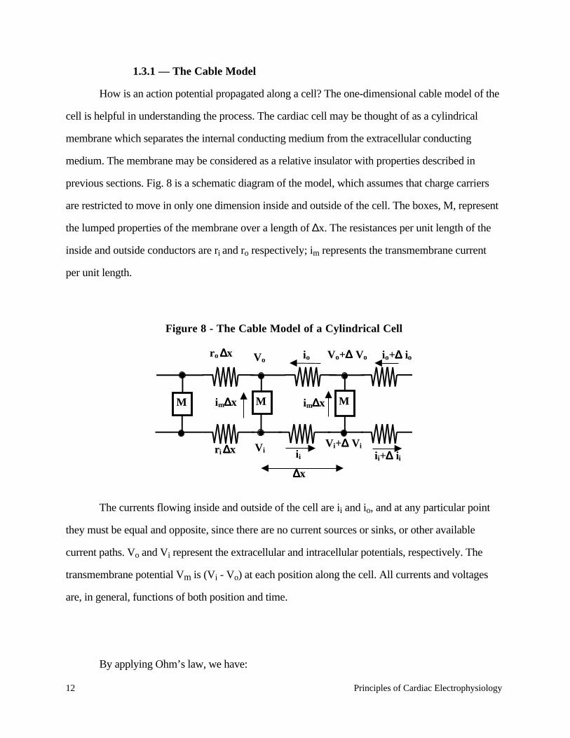
1.3.1 — The Cable Model
How is an action potential propagated along a cell? The one-dimensional cable model of the
cell is helpful in understanding the process. The cardiac cell may be thought of as a cylindrical
membrane which separates the internal conducting medium from the extracellular conducting
medium. The membrane may be considered as a relative insulator with properties described in
previous sections. Fig. 8 is a schematic diagram of the model, which assumes that charge carriers
are restricted to move in only one dimension inside and outside of the cell. The boxes, M, represent
the lumped properties of the membrane over a length of ∆x. The resistances per unit length of the
inside and outside conductors are ri and ro respectively; im represents the transmembrane current
per unit length.
Figure 8 - The Cable Model of a Cylindrical Cell
M M M
r o ∆∆∆∆x
r i ∆∆∆∆x V i
Vo
im∆∆∆∆x
i i
io Vo+∆∆∆∆ Vo
Vi+∆∆∆∆ Vi
im∆∆∆∆x
i i+∆∆∆∆ ii∆∆∆∆x
io+∆∆∆∆ io
The currents flowing inside and outside of the cell are ii and io, and at any particular point
they must be equal and opposite, since there are no current sources or sinks, or other available
current paths. Vo and Vi represent the extracellular and intracellular potentials, respectively. The
transmembrane potential Vm is (Vi - Vo) at each position along the cell. All currents and voltages
are, in general, functions of both position and time.
By applying Ohm’s law, we have:
Principles of Cardiac Electrophysiology 13
i i r i∆x = −∆V i (5)
In the limit as ∆x → 0 this becomes:
∂V i
∂x= −i i r i (6)
By similar reasoning applied to the outer conductor, we obtain
∂V o
∂x= i oro = i i ro (7)
By analyzing current flows at any node, we observe that
∆i i = −i m∆x (8)
or in the limit:
∂i i
∂x= −i m (9)
Recalling the definition of Vm, and using (6) and (7)
∂V m
∂x= ∂
∂xV i − V o( ) = ∂V i
∂x− ∂V o
∂x= −i i r i + r0( )
i i = − 1r i + ro( )
∂V m
∂x
(10)
Differentiating and substituting into (9) we obtain
i m = 1r i + ro( )
∂2V m
∂x2 (11)
The membrane current per unit length is given by:
i m = Cm
∂V m
∂t+ V m
rm
(12)
14 Principles of Cardiac Electrophysiology
where Cm is the membrane capacitance per unit length and rm is the equivalent membrane resistance
per unit length. Substituting equation (12) into equation (11) results in the differential equation:
∂2V m x, t( )∂x2 = ro + r i( ) Cm
∂V m
∂t+ V m
rm
(13)
1.3.1.1 The Space Constant
This equation may be solved simply for the time invariant case ∂V m
∂t= 0
to yield the
variation of membrane potential with length resulting from a fixed initial transmembrane potential
V0 at one point (x=0) on an infinitely long strip of muscle cells.
V m x( ) = V 0e−x λ (14)
where λ = rm
r i + ro
.
The membrane current, im, will have the same functional form as Vm. λ is the so-called
“space constant,” and is a measure of the distance from the origin at which the membrane potential
(or current) falls to l/e of its initial value.1
1rm, ri, ro have been defined in terms associated with a particular cell. In order to account for geometricfactors, it is useful to use units for conductivities which are geometry-independent. We will also simplify theexpressions by assuming that ro<< ri.
Define: r i = rπa2 where ρ is the resistivity (Ω - cm) of the internal media.
rm = Rm2πa
where Rm is the transverse membrane resistivity in Ω - cm2.
cm =2πaCm where Cm = capacitance per unit area
It follows that λ = aRm2ρ .
Principles of Cardiac Electrophysiology 15
The transmembrane current depolarizes the membrane ahead of the action potential, and
thereby propagates the impulse down the cell. The current also flows from one cell to the next via
the low-resistance nexi, and thus the action potential spreads directly from cell to cell. The velocity
of propagation increases with increasing cell diameter, action potential amplitude, and the initial rate
of the rise of the action potential. The resistance of the nexi also has a major impact on conduction
velocity: increased resistance slows conduction velocity.
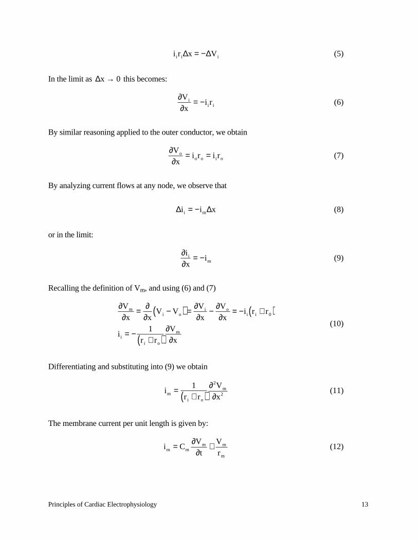
1.4 Automaticity
A number of cardiac cells display the property of automaticity — that is, they have the
ability to spontaneously generate propagated action potentials, and function as pacemaker cells.
Such cells are found in the SA node, the specialized conduction systems of the atria and ventricles,
and in the AV nodal region. In automatic cells, the diastolic (phase 4) potential is not stable, but
shows spontaneous depolarization (Fig. 9).
Figure 9Diagram of the Transmembrane Potential of an Automatic Cell
16 Principles of Cardiac Electrophysiology
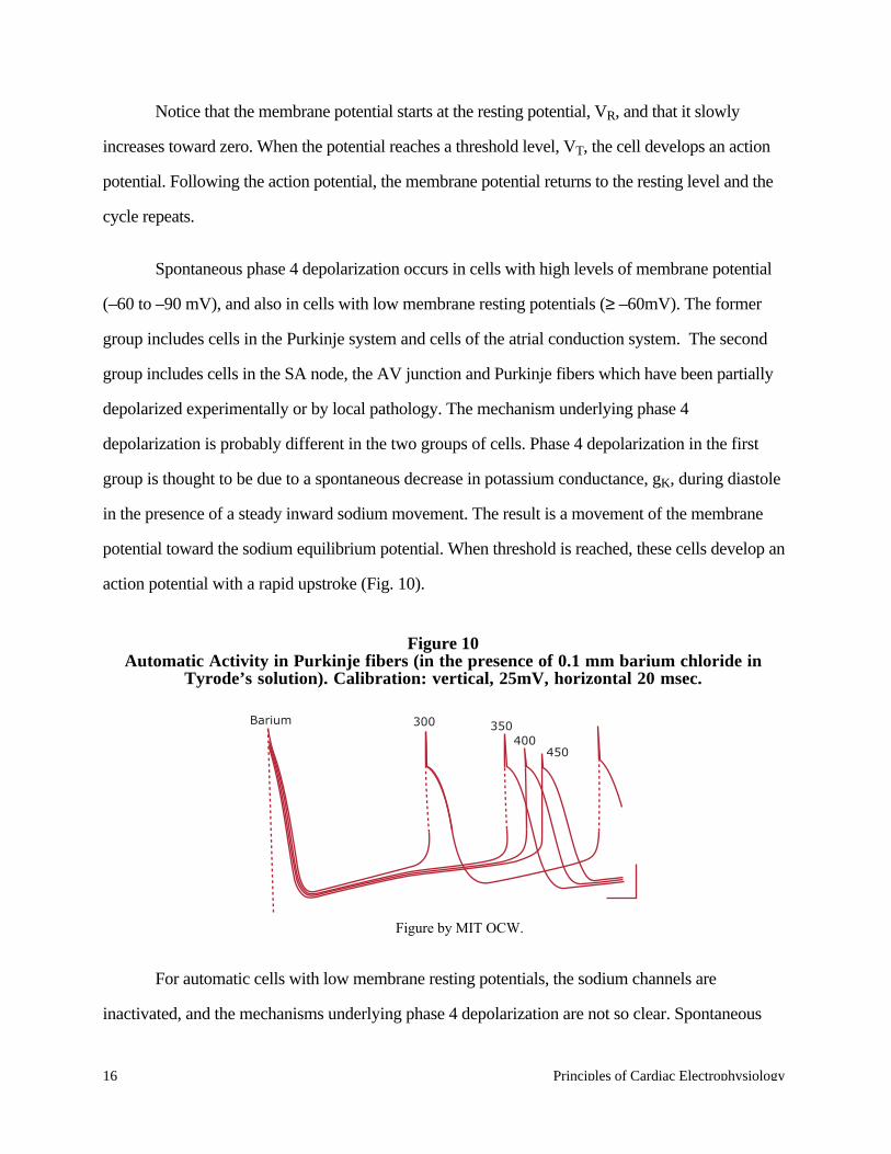
Notice that the membrane potential starts at the resting potential, VR, and that it slowly
increases toward zero. When the potential reaches a threshold level, VT, the cell develops an action
potential. Following the action potential, the membrane potential returns to the resting level and the
cycle repeats.
Spontaneous phase 4 depolarization occurs in cells with high levels of membrane potential
(–60 to –90 mV), and also in cells with low membrane resting potentials (≥ –60mV). The former
group includes cells in the Purkinje system and cells of the atrial conduction system. The second
group includes cells in the SA node, the AV junction and Purkinje fibers which have been partially
depolarized experimentally or by local pathology. The mechanism underlying phase 4
depolarization is probably different in the two groups of cells. Phase 4 depolarization in the first
group is thought to be due to a spontaneous decrease in potassium conductance, gK, during diastole
in the presence of a steady inward sodium movement. The result is a movement of the membrane
potential toward the sodium equilibrium potential. When threshold is reached, these cells develop an
action potential with a rapid upstroke (Fig. 10).
Figure 10Automatic Activity in Purkinje fibers (in the presence of 0.1 mm barium chloride in
Tyrode’s solution). Calibration: vertical, 25mV, horizontal 20 msec.
For automatic cells with low membrane resting potentials, the sodium channels are
inactivated, and the mechanisms underlying phase 4 depolarization are not so clear. Spontaneous
Barium 300 400
350
450
Figure by MIT OCW.
Principles of Cardiac Electrophysiology 17
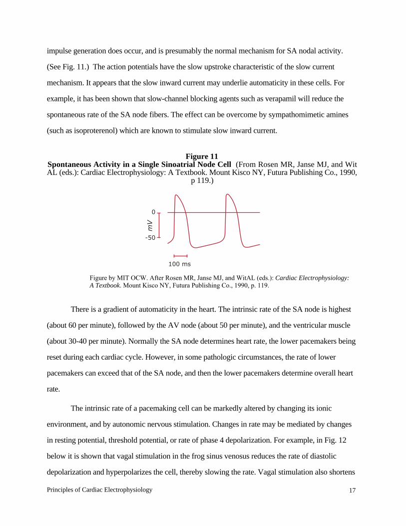
impulse generation does occur, and is presumably the normal mechanism for SA nodal activity.
(See Fig. 11.) The action potentials have the slow upstroke characteristic of the slow current
mechanism. It appears that the slow inward current may underlie automaticity in these cells. For
example, it has been shown that slow-channel blocking agents such as verapamil will reduce the
spontaneous rate of the SA node fibers. The effect can be overcome by sympathomimetic amines
(such as isoproterenol) which are known to stimulate slow inward current.
Figure 11Spontaneous Activity in a Single Sinoatrial Node Cell (From Rosen MR, Janse MJ, and WitAL (eds.): Cardiac Electrophysiology: A Textbook. Mount Kisco NY, Futura Publishing Co., 1990,
p 119.)
There is a gradient of automaticity in the heart. The intrinsic rate of the SA node is highest
(about 60 per minute), followed by the AV node (about 50 per minute), and the ventricular muscle
(about 30-40 per minute). Normally the SA node determines heart rate, the lower pacemakers being
reset during each cardiac cycle. However, in some pathologic circumstances, the rate of lower
pacemakers can exceed that of the SA node, and then the lower pacemakers determine overall heart
rate.
The intrinsic rate of a pacemaking cell can be markedly altered by changing its ionic
environment, and by autonomic nervous stimulation. Changes in rate may be mediated by changes
in resting potential, threshold potential, or rate of phase 4 depolarization. For example, in Fig. 12
below it is shown that vagal stimulation in the frog sinus venosus reduces the rate of diastolic
depolarization and hyperpolarizes the cell, thereby slowing the rate. Vagal stimulation also shortens
0
-50
100 ms
mV
Figure by MIT OCW. After Rosen MR, Janse MJ, and WitAL (eds.): Cardiac Electrophysiology:A Textbook. Mount Kisco NY, Futura Publishing Co., 1990, p. 119.
18 Principles of Cardiac Electrophysiology
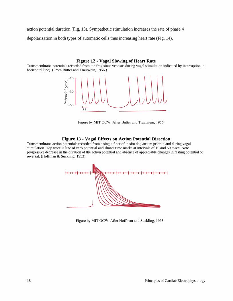
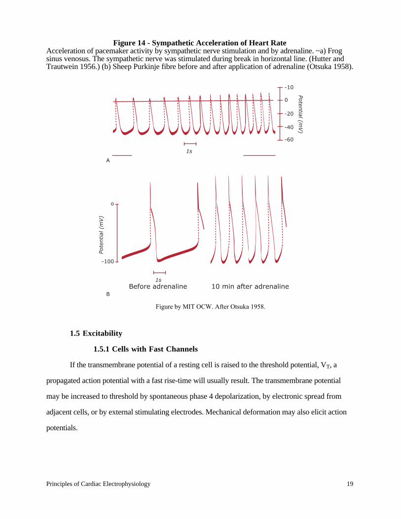
action potential duration (Fig. 13). Sympathetic stimulation increases the rate of phase 4
depolarization in both types of automatic cells thus increasing heart rate (Fig. 14).
Figure 12 - Vagal Slowing of Heart RateTransmembrane potentials recorded from the frog sinus venosus during vagal stimulation indicated by interruption inhorizontal line). (From Butter and Trautwein, 1956.)
Figure 13 - Vagal Effects on Action Potential DirectionTransmembrane action potentials recorded from a single fiber of in situ dog atrium prior to and during vagalstimulation. Top trace is line of zero potential and shows time marks at intervals of 10 and 50 msec. Noteprogressive decrease in the duration of the action potential and absence of appreciable changes in resting potential orreversal. (Hoffman & Suckling, 1953).
-10
-30
-50Pote
ntial
(m
V)
1s
Figure by MIT OCW. After Butter and Trautwein, 1956.
Figure by MIT OCW. After Hoffman and Suckling, 1953.
Principles of Cardiac Electrophysiology 19
Figure 14 - Sympathetic Acceleration of Heart RateAcceleration of pacemaker activity by sympathetic nerve stimulation and by adrenaline. ~a) Frogsinus venosus. The sympathetic nerve was stimulated during break in horizontal line. (Hutter andTrautwein 1956.) (b) Sheep Purkinje fibre before and after application of adrenaline (Otsuka 1958).
1.5 Excitability
1.5.1 Cells with Fast Channels
If the transmembrane potential of a resting cell is raised to the threshold potential, VT, a
propagated action potential with a fast rise-time will usually result. The transmembrane potential
may be increased to threshold by spontaneous phase 4 depolarization, by electronic spread from
adjacent cells, or by external stimulating electrodes. Mechanical deformation may also elicit action
potentials.
o
-100
1s
1s
Pote
ntial
(m
V)
Poten
tial (mV)
Before adrenaline 10 min after adrenaline
-10
0
-20
-40
-60
A
B
Figure by MIT OCW. After Otsuka 1958.
20 Principles of Cardiac Electrophysiology
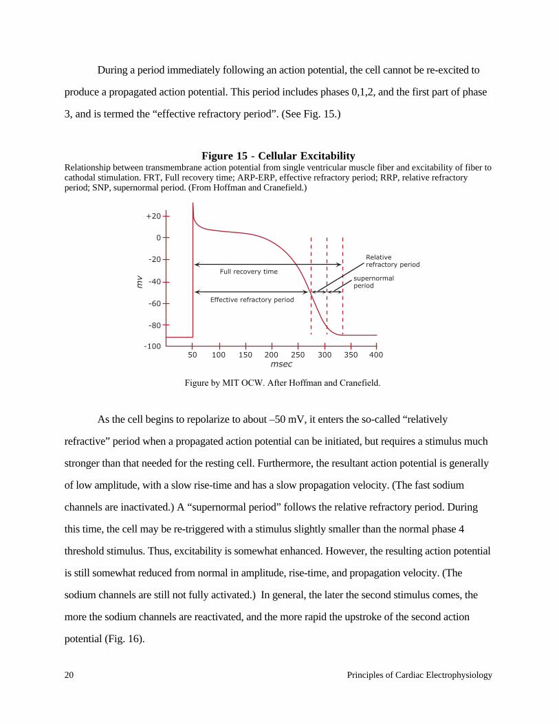
During a period immediately following an action potential, the cell cannot be re-excited to
produce a propagated action potential. This period includes phases 0,1,2, and the first part of phase
3, and is termed the “effective refractory period”. (See Fig. 15.)
Figure 15 - Cellular ExcitabilityRelationship between transmembrane action potential from single ventricular muscle fiber and excitability of fiber tocathodal stimulation. FRT, Full recovery time; ARP-ERP, effective refractory period; RRP, relative refractoryperiod; SNP, supernormal period. (From Hoffman and Cranefield.)
As the cell begins to repolarize to about –50 mV, it enters the so-called “relatively
refractive” period when a propagated action potential can be initiated, but requires a stimulus much
stronger than that needed for the resting cell. Furthermore, the resultant action potential is generally
of low amplitude, with a slow rise-time and has a slow propagation velocity. (The fast sodium
channels are inactivated.) A “supernormal period” follows the relative refractory period. During
this time, the cell may be re-triggered with a stimulus slightly smaller than the normal phase 4
threshold stimulus. Thus, excitability is somewhat enhanced. However, the resulting action potential
is still somewhat reduced from normal in amplitude, rise-time, and propagation velocity. (The
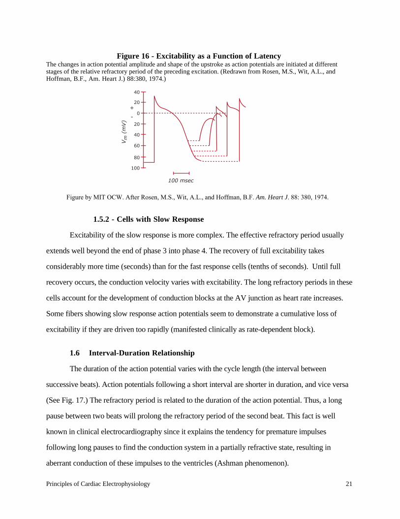
sodium channels are still not fully activated.) In general, the later the second stimulus comes, the
more the sodium channels are reactivated, and the more rapid the upstroke of the second action
potential (Fig. 16).
+20
0
-20
Full recovery time
-40
-60
-80
-10050 100 150 200 250 300 350 400
mv
msec
Effective refractory period
Relative refractory period
supernormal period
Figure by MIT OCW. After Hoffman and Cranefield.
Principles of Cardiac Electrophysiology 21
Figure 16 - Excitability as a Function of LatencyThe changes in action potential amplitude and shape of the upstroke as action potentials are initiated at differentstages of the relative refractory period of the preceding excitation. (Redrawn from Rosen, M.S., Wit, A.L., andHoffman, B.F., Am. Heart J.) 88:380, 1974.)
1.5.2 - Cells with Slow Response
Excitability of the slow response is more complex. The effective refractory period usually
extends well beyond the end of phase 3 into phase 4. The recovery of full excitability takes
considerably more time (seconds) than for the fast response cells (tenths of seconds). Until full
recovery occurs, the conduction velocity varies with excitability. The long refractory periods in these
cells account for the development of conduction blocks at the AV junction as heart rate increases.
Some fibers showing slow response action potentials seem to demonstrate a cumulative loss of
excitability if they are driven too rapidly (manifested clinically as rate-dependent block).
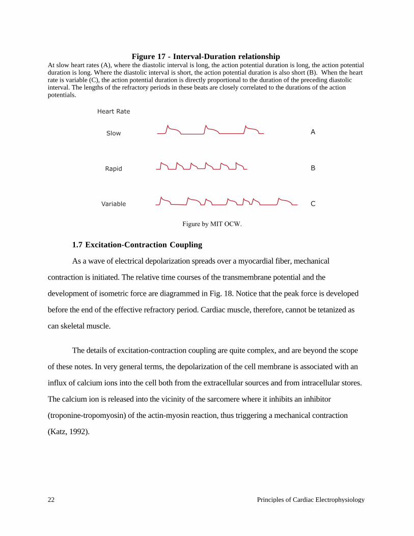
1.6 Interval-Duration Relationship
The duration of the action potential varies with the cycle length (the interval between
successive beats). Action potentials following a short interval are shorter in duration, and vice versa
(See Fig. 17.) The refractory period is related to the duration of the action potential. Thus, a long
pause between two beats will prolong the refractory period of the second beat. This fact is well
known in clinical electrocardiography since it explains the tendency for premature impulses
following long pauses to find the conduction system in a partially refractive state, resulting in
aberrant conduction of these impulses to the ventricles (Ashman phenomenon).
40
20+
-0
20
40
60
80
100
100 msec
Vm
(m
V)
Figure by MIT OCW. After Rosen, M.S., Wit, A.L., and Hoffman, B.F. Am. Heart J. 88: 380, 1974.
22 Principles of Cardiac Electrophysiology
Figure 17 - Interval-Duration relationshipAt slow heart rates (A), where the diastolic interval is long, the action potential duration is long, the action potentialduration is long. Where the diastolic interval is short, the action potential duration is also short (B). When the heartrate is variable (C), the action potential duration is directly proportional to the duration of the preceding diastolicinterval. The lengths of the refractory periods in these beats are closely correlated to the durations of the actionpotentials.
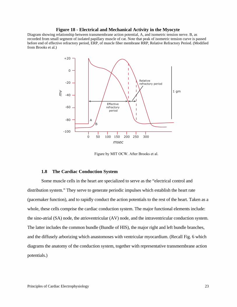
1.7 Excitation-Contraction Coupling
As a wave of electrical depolarization spreads over a myocardial fiber, mechanical
contraction is initiated. The relative time courses of the transmembrane potential and the
development of isometric force are diagrammed in Fig. 18. Notice that the peak force is developed
before the end of the effective refractory period. Cardiac muscle, therefore, cannot be tetanized as
can skeletal muscle.
The details of excitation-contraction coupling are quite complex, and are beyond the scope
of these notes. In very general terms, the depolarization of the cell membrane is associated with an
influx of calcium ions into the cell both from the extracellular sources and from intracellular stores.
The calcium ion is released into the vicinity of the sarcomere where it inhibits an inhibitor
(troponine-tropomyosin) of the actin-myosin reaction, thus triggering a mechanical contraction
(Katz, 1992).
Heart Rate
A
B
C
Slow
Rapid
Variable
Figure by MIT OCW.
Principles of Cardiac Electrophysiology 23
Figure 18 - Electrical and Mechanical Activity in the MyocyteDiagram showing relationship between transmembrane action potential, A, and isometric tension nerve. B, asrecorded from small segment of isolated papillary muscle of cat. Note that peak of isometric tension curve is passedbefore end of effective refractory period, ERP, of muscle fiber membrane RRP, Relative Refractory Period. (Modifiedfrom Brooks et al.)
1.8 The Cardiac Conduction System
Some muscle cells in the heart are specialized to serve as the “electrical control and
distribution system.” They serve to generate periodic impulses which establish the heart rate
(pacemaker function), and to rapidly conduct the action potentials to the rest of the heart. Taken as a
whole, these cells comprise the cardiac conduction system. The major functional elements include:
the sino-atrial (SA) node, the atrioventricular (AV) node, and the intraventricular conduction system.
The latter includes the common bundle (Bundle of HIS), the major right and left bundle branches,
and the diffusely arborizing which anastomoses with ventricular myocardium. (Recall Fig. 6 which
diagrams the anatomy of the conduction system, together with representative transmembrane action
potentials.)
+20
0
-20
-40
AB
-60
-80
0 50 100 150 200 250 300
-100
1 gm
mv
msec
Effective refractory
period
Relative refractory period
Figure by MIT OCW. After Brooks et al.
24 Principles of Cardiac Electrophysiology
The cardiac impulse normally arises in the SA node. This structure is a region of specialized
muscle cells located in the right atrium near the entrance of the superior vena cava. Sympathetic and
parasympathetic fibers richly innervate this region, and may speed or slow the rate of impulse
formation to vary heart rate. Action potentials spread from the SA node throughout the atria with a
propagation velocity of about 1 meter/second. Electrophysiologic studies have suggested the
existence of at least three routes of preferential conduction in the atria with propagation velocities
somewhat greater than in non-specialized atrial tissue. Although some workers doubt the existence
of specific anatomically differentiated bundles, they are often referred to as the internodal tracts, and
serve to channel the impulse from the SA node to the atrio-ventricular (AV node). Cells in the
internodal tracts may also function as pacemakers under the right conditions.
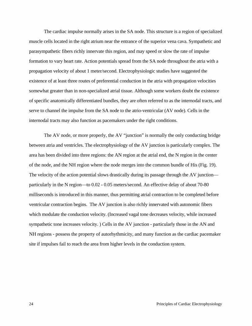
The AV node, or more properly, the AV “junction” is normally the only conducting bridge
between atria and ventricles. The electrophysiology of the AV junction is particularly complex. The
area has been divided into three regions: the AN region at the atrial end, the N region in the center
of the node, and the NH region where the node merges into the common bundle of His (Fig. 19).
The velocity of the action potential slows drastically during its passage through the AV junction—
particularly in the N region—to 0.02 - 0.05 meters/second. An effective delay of about 70-80
milliseconds is introduced in this manner, thus permitting atrial contraction to be completed before
ventricular contraction begins. The AV junction is also richly innervated with autonomic fibers
which modulate the conduction velocity. (Increased vagal tone decreases velocity, while increased
sympathetic tone increases velocity. ) Cells in the AV junction - particularly those in the AN and
NH regions - possess the property of autorhythmicity, and many function as the cardiac pacemaker
site if impulses fail to reach the area from higher levels in the conduction system.
Principles of Cardiac Electrophysiology 25
Figure 19 - Atrioventricular conduction system.The AV node can be divided functionally into three regions: AN (upper, or atrionodal), N (middle, or nodal), and NH(lower, or nodal-His bundle). (From Katz, Arnold M., Physiology of the Heart (New York: Raven Press Books,1992), p. 467.)
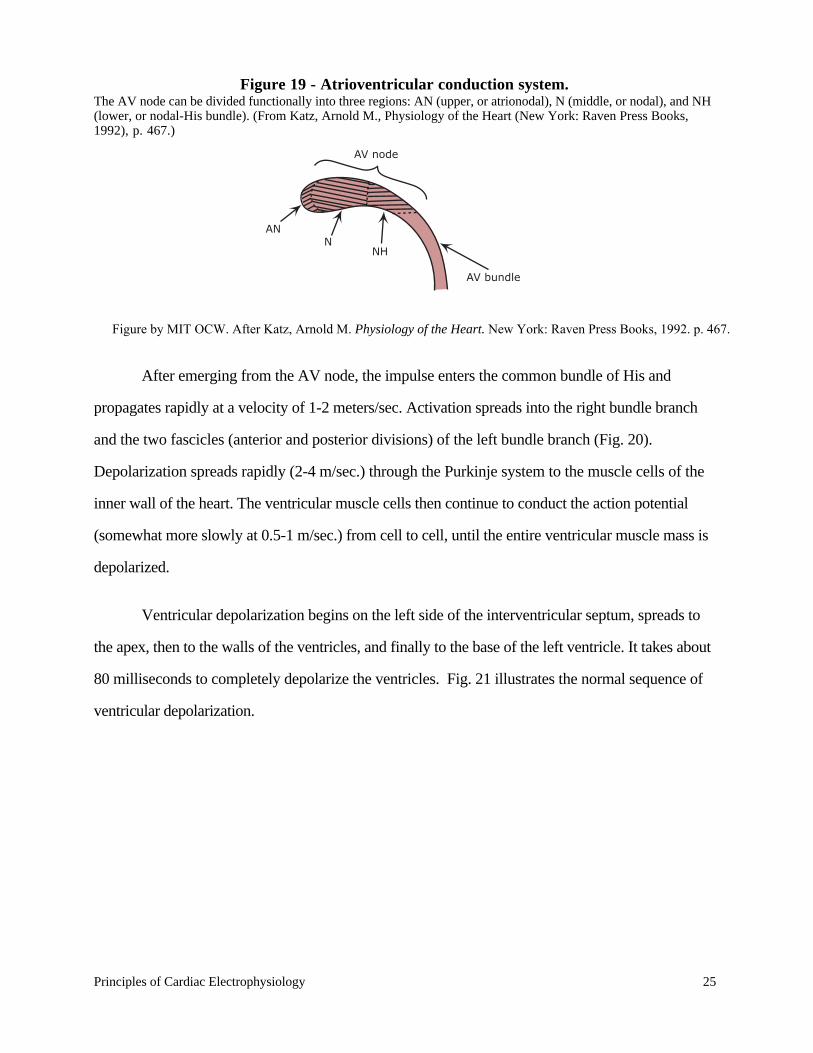
After emerging from the AV node, the impulse enters the common bundle of His and
propagates rapidly at a velocity of 1-2 meters/sec. Activation spreads into the right bundle branch
and the two fascicles (anterior and posterior divisions) of the left bundle branch (Fig. 20).
Depolarization spreads rapidly (2-4 m/sec.) through the Purkinje system to the muscle cells of the
inner wall of the heart. The ventricular muscle cells then continue to conduct the action potential
(somewhat more slowly at 0.5-1 m/sec.) from cell to cell, until the entire ventricular muscle mass is
depolarized.
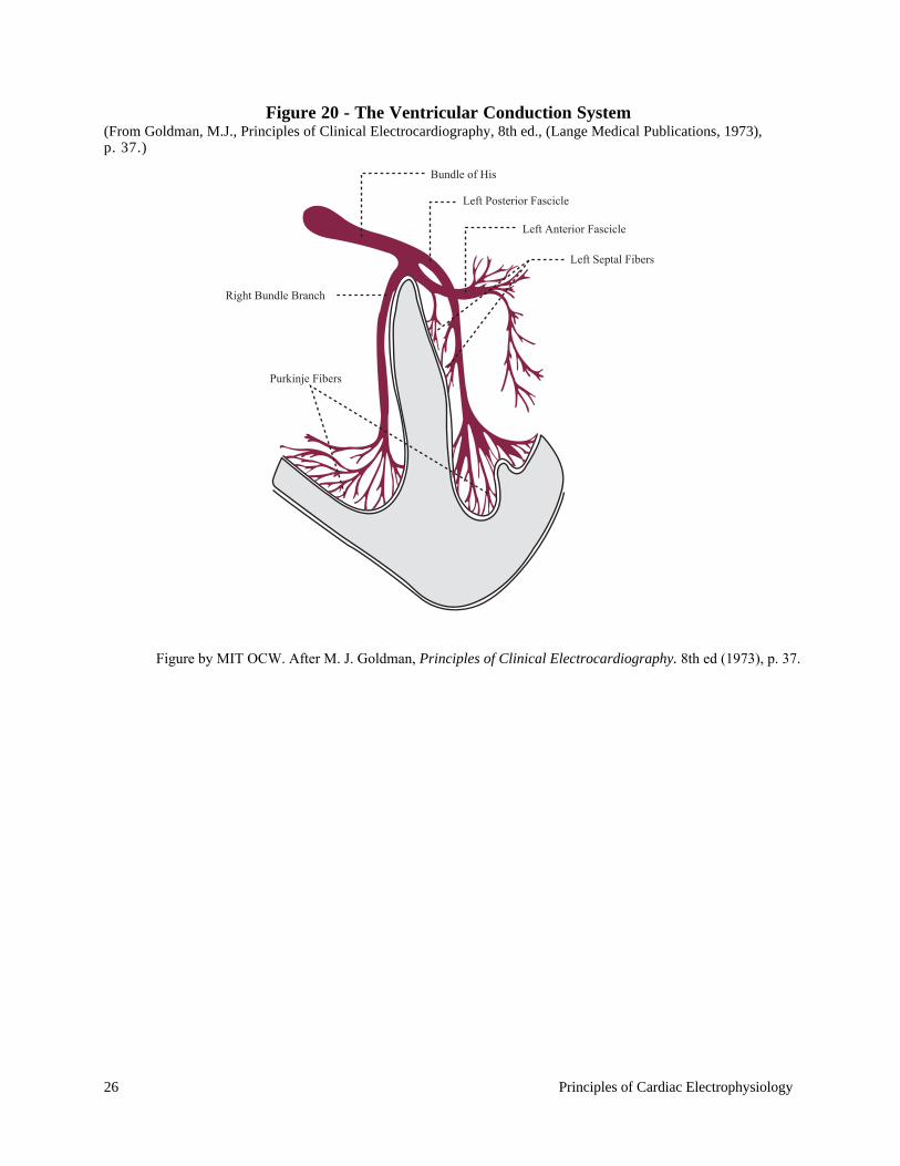
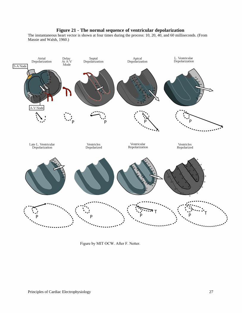
Ventricular depolarization begins on the left side of the interventricular septum, spreads to
the apex, then to the walls of the ventricles, and finally to the base of the left ventricle. It takes about
80 milliseconds to completely depolarize the ventricles. Fig. 21 illustrates the normal sequence of
ventricular depolarization.
AV node
AV bundle
NNH
AN
Figure by MIT OCW. After Katz, Arnold M. Physiology of the Heart. New York: Raven Press Books, 1992. p. 467.
26 Principles of Cardiac Electrophysiology
Figure 20 - The Ventricular Conduction System(From Goldman, M.J., Principles of Clinical Electrocardiography, 8th ed., (Lange Medical Publications, 1973),p. 37.)
Bundle of His
Left Posterior Fascicle
Left Anterior Fascicle
Left Septal Fibers
Right Bundle Branch
Purkinje Fibers
Figure by MIT OCW. After M. J. Goldman, Principles of Clinical Electrocardiography. 8th ed (1973), p. 37.
Principles of Cardiac Electrophysiology 27
Figure 21 - The normal sequence of ventricular depolarizationThe instantaneous heart vector is shown at four times during the process: 10, 20, 40, and 60 milliseconds. (FromMassie and Walsh, 1960.)
Figure by MIT OCW. After F. Netter.

28 Principles of Cardiac Electrophysiology
2. THE PHYSICAL BASIS OF ELECTROCARDIOGRAPHY
2.1 lntroduction
In the preceding section, we reviewed the electrophysiology of myocardial cells. As a result
of the electrical activity of those cells, current flows within the body and potential differences are
established on the surface of the skin which can be measured using suitable equipment. The
graphical recording of these body surface potentials as a function of time produces the
electrocardiogram (ECG). Fig. 22 illustrates a single-lead scalar electrocardiogram.
Figure 22 - Example of a Scalar Electrocardiogram(From Philips and Feeney, The Cardiac Rhythms: A Systematic Approach to Interpretation, Philadelphia:W.B.Saunders, 1980, p. 36.)
In this section we wish to examine the relationship between the cellular events and the body
surface potentials. The clinician who uses the electrocardiogram as a diagnostic test wishes to
determine cardiac abnormalities from the body surface potentials. Given a distribution of body
surface potentials, can we specify the detailed electrophysiologic behavior of the source?
Unfortunately this “inverse” problem does not have a unique solution as demonstrated in 1853 by
Hermann von Helmholz. It is not, in general, possible to uniquely specify the characteristics of a
current generator from the external potential measurements alone.
The “forward” problem is more tractable: given knowledge of the heart generator, can the
body surface potentials be specified? If the transmembrane potentials of all the cells within the heart
were known, can a mathematical expression be found to specify the extracellular potentials
everywhere in the surrounding space? A complete solution would include details of tissue geometry
Figure courtesy of PhysioNet (http://www.physionet.org).
Principles of Cardiac Electrophysiology 29
and electrical properties, as well as an exhaustive description of the detailed electrical activity of the
heart. The investigation of the forward problem has frequently employed the use of physical and/or
mathematical models. A number of investigators have studied models of the human torso in which
they have imbedded well-defined electrical sources. The models are typically plastic containers
shaped in the form of a human torso and filled with a conductive liquid medium. Inhomogeneities
of the conducting media (such as lungs) are sometimes modeled by bags of lower conductivity
material such as sand. By placing well-defined electrical dipole sources within the model torso, the
relationship between the cardiac generator and body surface potentials may be studied.
Mathematical models have been proposed as well. The heart is typically represented by a number of
spatially distributed dipole sources imbedded in a conductive medium of variable complexity.
Computer simulations have made it possible to develop impressive demonstrations using hundreds
of dipoles, and synthesizing the resultant body surface potential distributions (Miller, Geselowitz,
1978). The simplest mathematical model for relating the cardiac generator to the body surface
potentials is the single dipole model. This simple model is an interesting and useful one which dates
back to the earliest days of human electrocardiography. It is still extremely useful in providing a
framework for the study of clinical electrocardiography and vectorcardiography.
2.2 The Dipole Model
The model has two components: a) a representation of the electrical activity of the heart
cells, and b) a representation of the geometry and electrical properties of the body. Having modeled
the source and the conductive body media, it is a straightforward task to develop the relationship
between source and surface potentials.
2.2.1 The Source
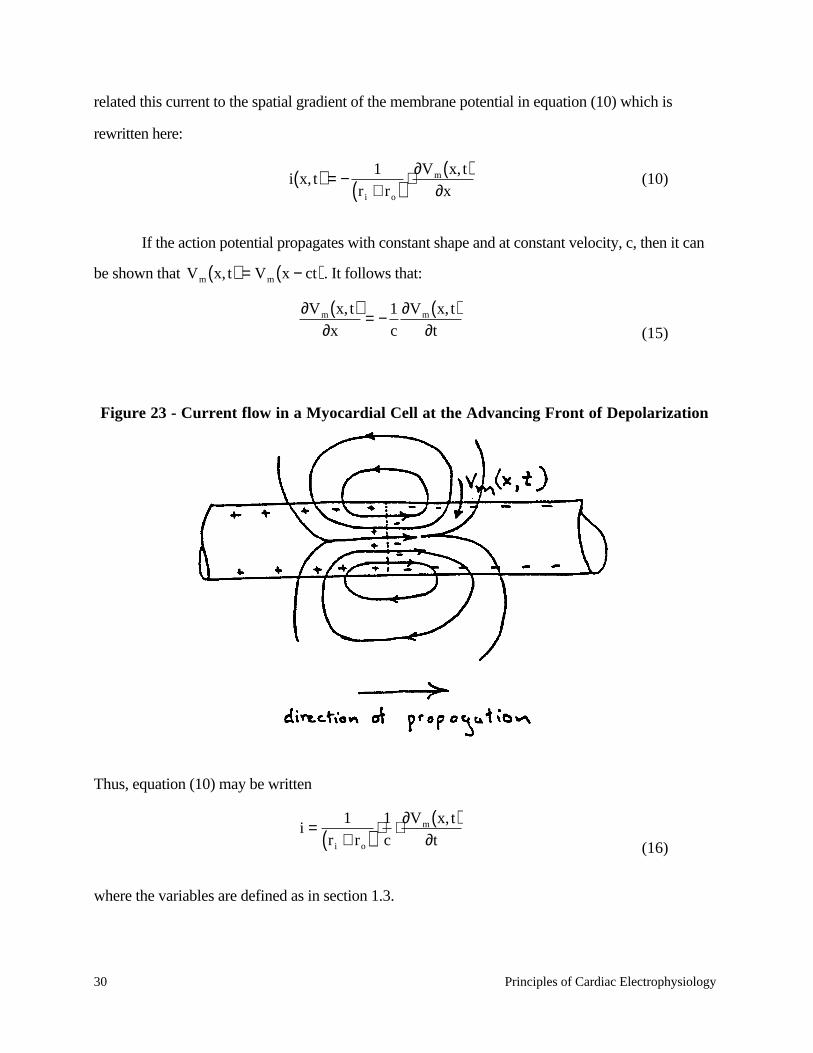
The smallest unit contributing to the ECG is the single myocardial cell. Fig. 23 shows such
a cell in which an action potential is propagating. The action potential is associated with a current,
i(x,t), within the cell flowing in the direction of propagation of the action potential. The cable model
30 Principles of Cardiac Electrophysiology
related this current to the spatial gradient of the membrane potential in equation (10) which is
rewritten here:
i x, t( ) = − 1r i + ro( ) ⋅ ∂V m x, t( )
∂x(10)
If the action potential propagates with constant shape and at constant velocity, c, then it can
be shown that V m x, t( ) = V m x − ct( ). It follows that:
∂V m x, t( )∂x
= − 1c
∂V m x, t( )∂t (15)
Figure 23 - Current flow in a Myocardial Cell at the Advancing Front of Depolarization
Thus, equation (10) may be written
i = 1r i + ro( ) ⋅ 1
c⋅ ∂V m x, t( )
∂t (16)
where the variables are defined as in section 1.3.
Principles of Cardiac Electrophysiology 31
We will consider the intracellular longitudinal current at the interface of normal and
depolarized tissue to be the elementary electrical source, which we will refer to as a current dipole.
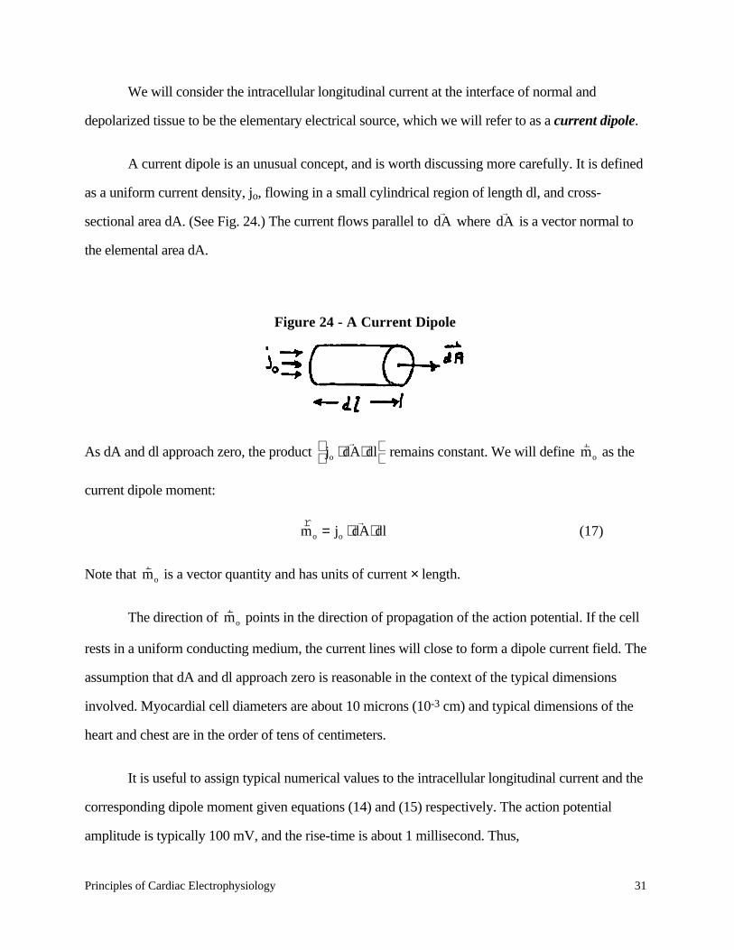
A current dipole is an unusual concept, and is worth discussing more carefully. It is defined
as a uniform current density, jo, flowing in a small cylindrical region of length dl, and cross-
sectional area dA. (See Fig. 24.) The current flows parallel to dA→
where dA→
is a vector normal to
the elemental area dA.
Figure 24 - A Current Dipole
As dA and dl approach zero, the product jo ⋅ dA→
⋅ dl
remains constant. We will define
rmo as the
current dipole moment:
rmo = jo ⋅ dA
→⋅ dl (17)
Note that rmo is a vector quantity and has units of current × length.
The direction of rmo points in the direction of propagation of the action potential. If the cell
rests in a uniform conducting medium, the current lines will close to form a dipole current field. The
assumption that dA and dl approach zero is reasonable in the context of the typical dimensions
involved. Myocardial cell diameters are about 10 microns (10-3 cm) and typical dimensions of the
heart and chest are in the order of tens of centimeters.
It is useful to assign typical numerical values to the intracellular longitudinal current and the
corresponding dipole moment given equations (14) and (15) respectively. The action potential
amplitude is typically 100 mV, and the rise-time is about 1 millisecond. Thus,
32 Principles of Cardiac Electrophysiology
∂V m
∂t =100 volts/ second
The velocity of propagation is roughly 100 cm/sec. in ventricular muscle. For simplicity we
will assume that r0 << ri. The resistance per unit length of the intracellular media, ri, can be
estimated by assuming a resistivity, ρ, of 100 ohm-cm, and a cellular cross-sectional area of
approximately 10-6 cm2. It follows that
ri = ρ/da =108 ohms/cm
The intracellular current then becomes
i =10-8 amperes
In order to calculate the magnitude of the dipole moment, mo, we require an estimate of dl,
the effective length of the source. Using the previous values of action potential velocity and
upstroke time, the estimate for dl is 10-l cm. Thus, the estimated magnitude of the dipole moment
would be:
|mo| ≈ 10-9 amp-cm
The heart’s total electrical activity at any instant of time may be represented by a distribution
of active current dipoles. In general, they will lie on an irregular surface corresponding to the
boundary between depolarized and polarized tissue.
If the heart were suspended in a homogeneous isotropic conducting medium, and were
observed from a distance large compared to its size, then all of the individual current dipoles may be
assumed to originate at the same point in space. The total electrical activity of the heat may then be
represented as a single equivalent dipole whose magnitude and direction is the vector summation of
all the individual dipole sources. The net equivalent dipole moment, rM , is commonly referred to as
Principles of Cardiac Electrophysiology 33
the “heart vector”. As cardiac depolarization spreads, the heart vector, rM changes in magnitude
and direction as a function of time. (Refer to Fig. 21 above.)
2.2.2 Electrical Properties of Tissue
The sources that characterize the electrical activity of the heart are immersed in the body, and
the resulting distribution of currents and potentials depends on the electrical properties of the torso.
These have been investigated and the following results have been determined.
Linearity : For the current densities produced by the heart, the body tissues may be
considered linear: that is, the potential gradient or electric field is everywhere proportional to the
current density.
rJ = σ
rE = −σ
r∇Φ (18)
where rJ ≡ current density, σ ≡ conductivity of the tissue,
rE ≡ electrical field, and Φ ≡
potential.
Homogeneity: Different tissues have conductivities which vary considerably from one
another. For example, blood has a conductivity approximately five times as great as other tissues,
and blood masses such as those within the ventricles and great vessels certainly introduce time-
varying inhomogeneities into the thorax. Likewise, lung tissue, although its average conductivity is
similar to other tissue, varies by a factor of five or so with respiration! Thus, the torso is far from a
homogeneous medium. Furthermore, its properties vary with time!
Anisotropy: An isotropic medium is one in which the properties are independent of
orientation or direction. Some tissues are reasonably isotropic in small regions, but not all. In
muscle, for example, the impedance along fibers is less than that measured across fibers. In
addition, the presence of structures such as high-conductivity cylindrical blood vessels, and low-
conductivity bronchi and bone make the thorax a highly anisotropic medium.
34 Principles of Cardiac Electrophysiology
Complex Impedance: In the frequency band of interest (0.1 - 103 Hz), the reactive
components of tissue impedance are sufficiently small that the chest may be considered purely
resistive.
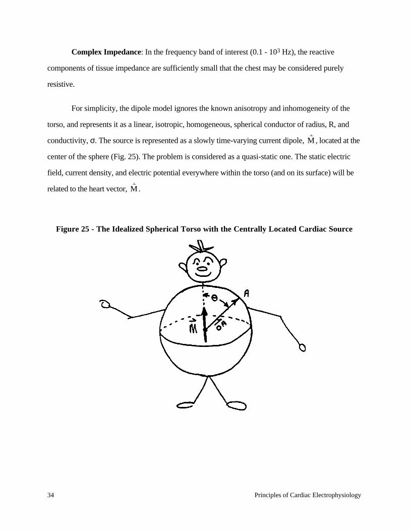
For simplicity, the dipole model ignores the known anisotropy and inhomogeneity of the
torso, and represents it as a linear, isotropic, homogeneous, spherical conductor of radius, R, and
conductivity, σ. The source is represented as a slowly time-varying current dipole, rM , located at the
center of the sphere (Fig. 25). The problem is considered as a quasi-static one. The static electric
field, current density, and electric potential everywhere within the torso (and on its surface) will be
related to the heart vector, rM .
Figure 25 - The Idealized Spherical Torso with the Centrally Located Cardiac Source
Principles of Cardiac Electrophysiology 35
2.2.3 Calculation of Potential within the Sphere
Within the sphere, equation (18) must hold. In addition, since there is no net generation of
charge anywhere,
r∇ ⋅
rJ = 0 (19)
By combining equations (18) and (19), Laplace’s equation for the potential is obtained:
∇2 ⋅ Φ = 0 (20)
By linearly combining general solutions to Laplace’s equation for a sphere in order to
satisfy the boundary conditions, the potential field may be found. The boundary conditions are:
1. The potential gradient in the radial direction must be zero at the surface of the sphere,
since no current is permitted to flow across the skin into air. Thus,
∂Φ r,θ( )∂r
= 0 at r = R (21)
2. We have assumed the source to be modeled by an equivalent current dipole of magnitude,
Mo, located at the center of the sphere. Hence, from the definition of equation (17), we must have:
M o =
rJ ⋅∫∫∫ dA
→dl (22)
One solution to Laplace’s equation is:
Φ1 r,θ( ) = Kcosθr2 (23)
The current densities may be obtained from the potential by using equation (18). Then,
using appropriate mathematical manipulations, the integration of equation (22) may be done in the
region of the source to evaluate K. The result yields:
Φ1 r,θ( ) = M o
4πσr2 cosθ (24)
36 Principles of Cardiac Electrophysiology
This solution, however, cannot satisfy the first boundary condition at the surface of the
sphere (eq. 21). We must add another solution to Laplace’s equation of the form:
Φ2 r,2( ) = A r cosθ (25)
Note that this potential disappears at r = 0, and thus will not alter our solution for K. The
new solution becomes:
Φ r,θ( ) = Φ1 r,θ( ) + Φ2 r,θ( )
The boundary condition of eq. (21) is satisfied when
A = 2Mo
4πσR3 (26)
Hence, the final solution for the potential within the sphere is:
Φ r,θ( ) = M o
4πσcosθ 1
r2 + 2rR3
(27)
2.2.4 The Surface Potentials
At the surface of the sphere (corresponding to the skin surface on the spherical torso), r=R
and
Φ R,θ( ) = 3Mo
4πσR2 cosθ (28)
where Mo is the magnitude of the equivalent heart vector, R is the radius of the sphere, and θ is the
angle between the point of observation an the direction of the heart vector.
Note that (28) could also be written in vector form
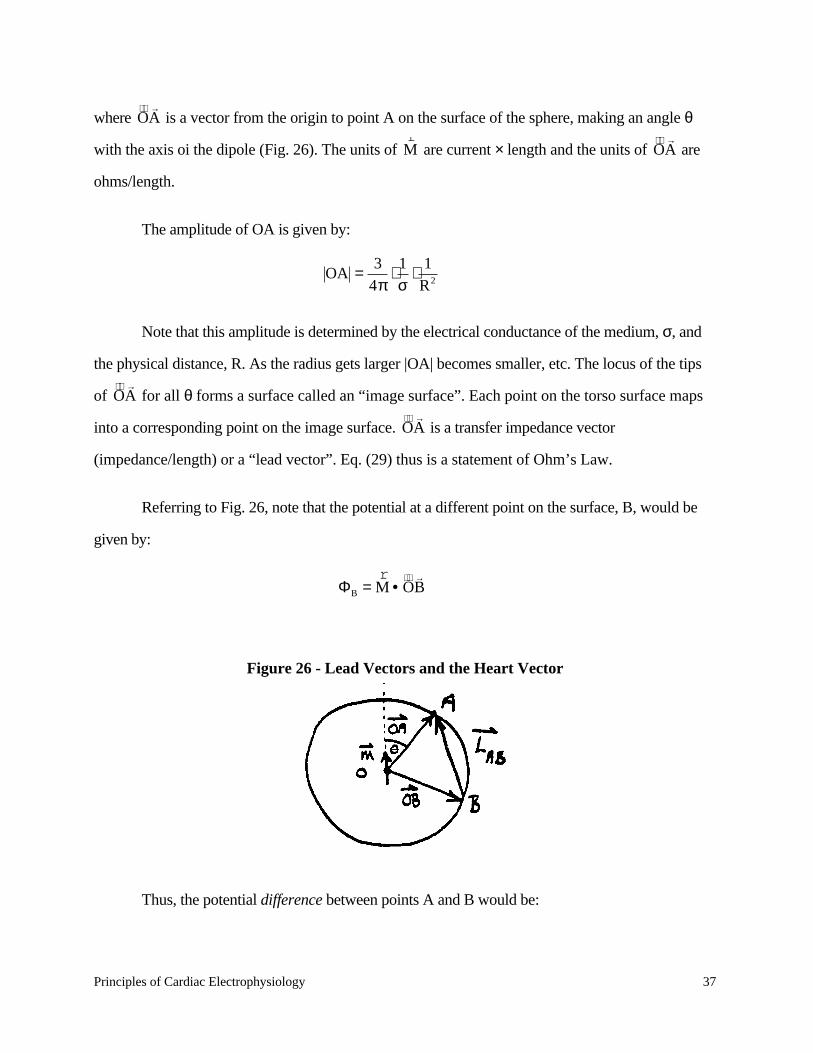
ΦA =rM • OA
→(29)
Principles of Cardiac Electrophysiology 37
where OA →
is a vector from the origin to point A on the surface of the sphere, making an angle θ
with the axis oi the dipole (Fig. 26). The units of rM are current × length and the units of OA
→ are
ohms/length.
The amplitude of OA is given by:
OA = 34π
⋅ 1σ
⋅ 1R2
Note that this amplitude is determined by the electrical conductance of the medium, σ, and
the physical distance, R. As the radius gets larger |OA| becomes smaller, etc. The locus of the tips
of OA →
for all θ forms a surface called an “image surface”. Each point on the torso surface maps
into a corresponding point on the image surface. OA →
is a transfer impedance vector
(impedance/length) or a “lead vector”. Eq. (29) thus is a statement of Ohm’s Law.
Referring to Fig. 26, note that the potential at a different point on the surface, B, would be
given by:
ΦB =rM • OB
→
Figure 26 - Lead Vectors and the Heart Vector
Thus, the potential difference between points A and B would be:
38 Principles of Cardiac Electrophysiology
VAB = ΦA − ΦB =rM • OA
→−rM • OB
→
=rM • OA
→− OB
→
=rM •
rL AB
The potential difference VAB is simply the scalar product of the heart vector with vector,
rL AB ,which is commonly referred to as the “lead vector”. The lead vector connects the points A and
B on the image surface.
Since in general rM is a function of time, the scalar potential difference VAB will also vary
with time. At any instant VAB will be the dot product, or projection of the instantaneous heart vector
on lead vector rL AB .
A wide variety of lead vectors may be formed by attaching electrodes to the body in various
positions. This subject will be covered in the next section.
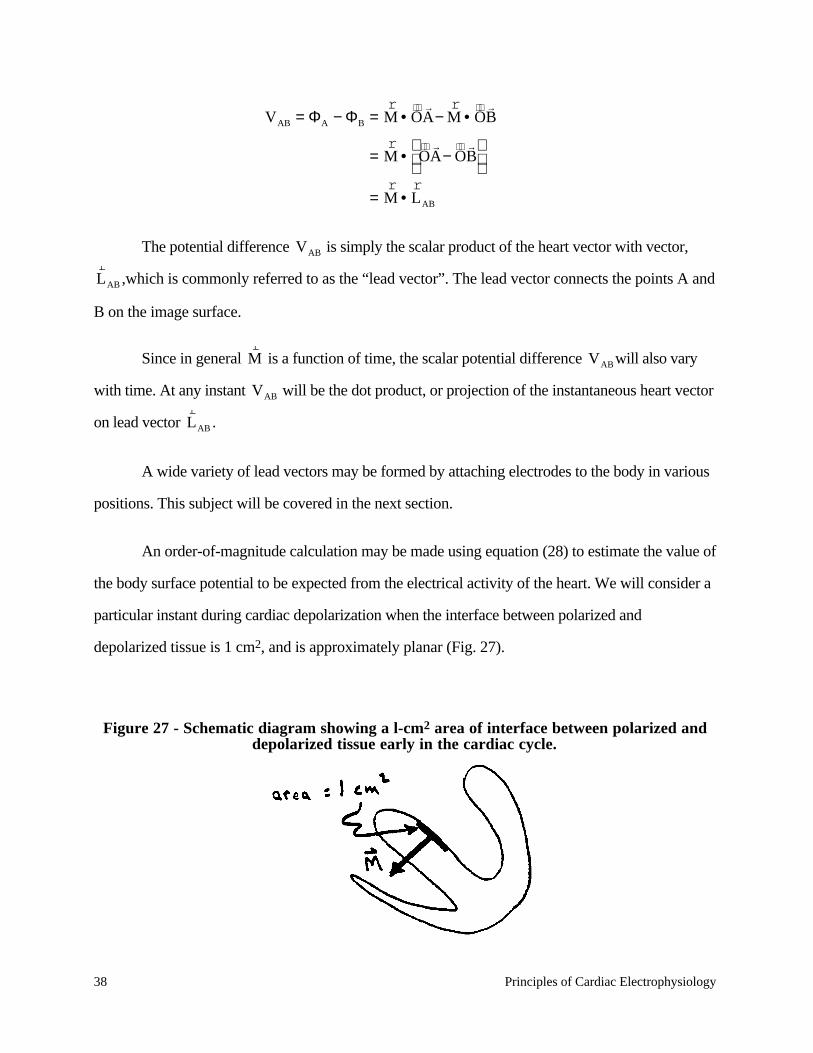
An order-of-magnitude calculation may be made using equation (28) to estimate the value of
the body surface potential to be expected from the electrical activity of the heart. We will consider a
particular instant during cardiac depolarization when the interface between polarized and
depolarized tissue is 1 cm2, and is approximately planar (Fig. 27).
Figure 27 - Schematic diagram showing a l-cm2 area of interface between polarized anddepolarized tissue early in the cardiac cycle.
Principles of Cardiac Electrophysiology 39
Since the cross-sectional area of individual cellular dipoles is 10-6 cm2, there will be approximately
106 of them in the interface region, and they will be parallel. Thus, the magnitude of net equivalent
heart dipole will be:
|Mo| = n|Mo| =106 × 10–9 =10–3 amp. cm.
We will assume a torso with a radius of 20 cm. and a conductivity, σ, of
3 × 10³ ohm-1-cm-1. The maximum surface potential would be
Φmax = 3M4πσR2 = 0.2 mV
Thus, the model predicts surface potentials in the order of fractions of millivolts, which
corresponds closely to experimentally measured values early in the sequence of ventricular
depolarization.
2.3 Lead Systems Used in Scalar Electrocardiography
Not surprisingly, the lead systems used in clinical practice utilize the limbs, since they are
convenient point of attachment for electrodes. In addition, chest electrodes are used to record
projections of the heart vector onto the horizontal plane.
2.3.1 Frontal Plane Scalar Leads
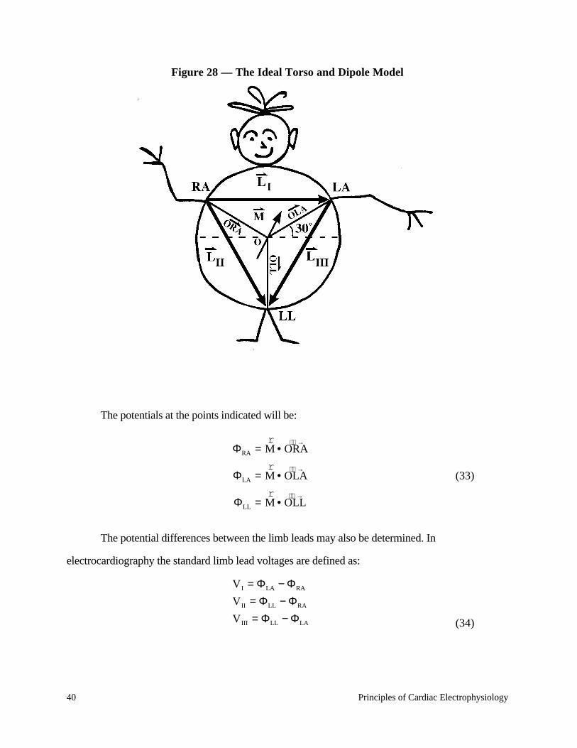
Suppose an electrode were attached to each arm and one leg of the subject (Fig. 28).
40 Principles of Cardiac Electrophysiology
Figure 28 — The Ideal Torso and Dipole Model
The potentials at the points indicated will be:
ΦRA =rM • ORA
→
ΦLA =rM • OLA
→
ΦLL =rM • OLL
→
(33)
The potential differences between the limb leads may also be determined. In
electrocardiography the standard limb lead voltages are defined as:
V I = ΦLA − ΦRA
V II = ΦLL − ΦRA
V III = ΦLL − ΦLA (34)
Principles of Cardiac Electrophysiology 41
From our previous considerations, and noting the definition of lead vectors rL I ,
rL II , and
rL III
from Fig. 28, we have:
V I =rM • OLA
→− ORA
→
=rM •
rL I
V II =rM •
rL II
V III =rM •
rL III
A simple way to visualize these results is to note that VI is simply the projection of the heart
vector rM on the lead vector
rL I .
It has been found useful in electrocardiography to define a “central terminal” by averaging
the potentials from the limb leads.
ΦCT = ΦRA + ΦLA + ΦLL
=rM • ORA
→+ OLA
→+ OLL
→
= 0
since the vectors in the parenthesis sum to zero. Using the central terminal as a reference, one may
now construct new lead vectors
V L = ΦLA − ΦCT = ΦLA =rM • OLA
→
V R = ΦRA =rM • ORA
→
V F = ΦLL =rM • OLL
→
(37)
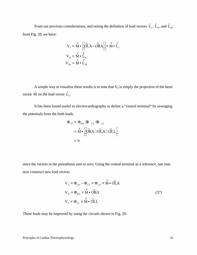
These leads may be improved by using the circuits shown in Fig. 29.
42 Principles of Cardiac Electrophysiology
Figure 29 — Standard Connections for Augmented Limb Leads
aVL = ΦLA − ΦRA + ΦLL
2
= 1.5VL
aVR = ΦRA − ΦLA + ΦLL
2
= 1.5VR
aVF = ΦLL − ΦLA + ΦRA
2
= 1.5VF
(38)
These leads are referred to as the augmented limb leads.
The complete set of frontal lead vectors is shown in Fig. 30 with all vectors drawn to pass
through the origin. It should be noted that the amplitudes of these lead vectors are not equal.
rL I ,
rL II ,
rL III = R 3 while the augmented leads are 1.5R. (This difference will be ignored.)
2.3.2 Precordial Leads
By using the “central terminal” as a reference electrode, and placing an exploring electrode
at various points on the chest, a variety of horizontal plane lead vectors may be obtained. In clinical
practice, six standard chest leads are used, and are termed V1, V2, …, V6. The placement of the
electrodes is shown in Fig. 31.
A complete scalar ECG, then, would consist of 12 leads - six frontal plane and six
precordial leads.
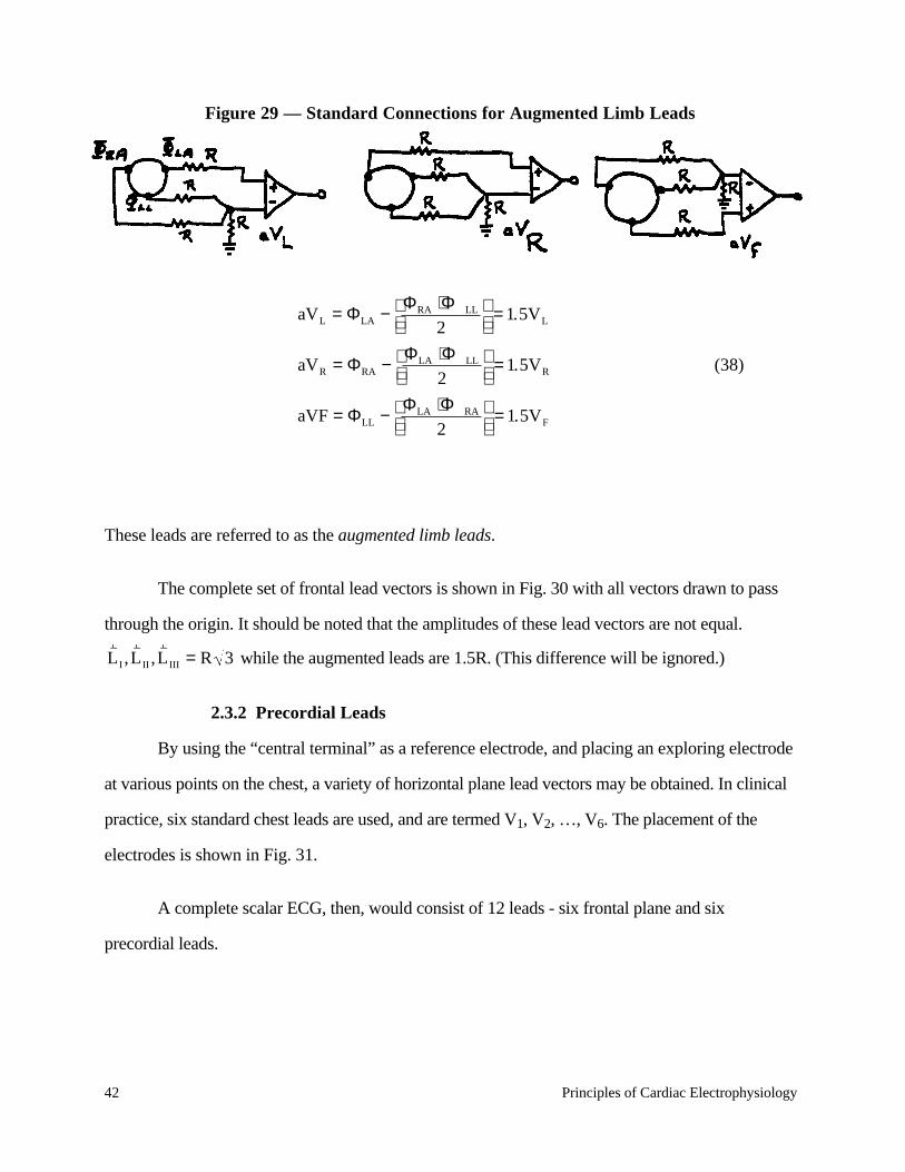
Principles of Cardiac Electrophysiology 43
Figure 30 — Frontal Plane Limb Leads
Figure 31 — The Six Standard Chest LeadsThe location of these leads is as follows:
V1: on the fourth intercostal space at the right sternal margin
V2: on the fourth intercostal space at the left sternal margin
V3: midway between leads V2 and V4
V4: on the fifth intercostal space at the midclavicular line
V5: on the anterior axillary line at the horizontal level of lead V4
V6: on the midaxillary line at the horizontal level of lead V4
-1200
-1500
aVR
aVF
aVL
I
IIIII
-900
-800
-300
+300
+600
+900+1200
+1500
1800 00
Figure by MIT OCW.
Figure by MIT OCW.
44 Principles of Cardiac Electrophysiology
2.4 Electrical Axis
The complete description of the source is a three-dimensional plot of the locus of the tip of
the equivalent heart vector. The same information could be presented in three two-dimensional plots
showing the projection of the locus on the horizontal, frontal, and sagittal planes. This type of
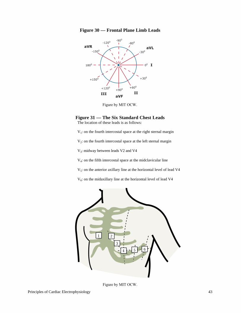
display is termed the vectorcardiogram. A typical frontal-plane loop is illustrated in Fig. 32.
Figure 32 — A Frontal Plane VCG Loop
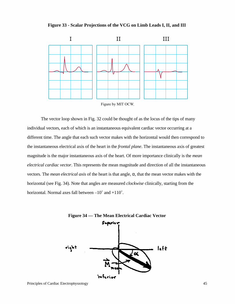
A waveform that would be recorded on lead I of the scalar ECG is simply the plot of the
projection of the loop onto rL I as a function of time. Similarly, the waveform that would be seen in
Lead II the projection of the loop onto rL II . These plots are shown in approximate form in Fig. 33.
I
aVRaVL
aVFIII
II
Mean TVector
Long Axisof QRS Loop
+
+ +
+
+
+
Figure by MIT OCW.
Principles of Cardiac Electrophysiology 45
Figure 33 - Scalar Projections of the VCG on Limb Leads I, II, and III
The vector loop shown in Fig. 32 could be thought of as the locus of the tips of many
individual vectors, each of which is an instantaneous equivalent cardiac vector occurring at a
different time. The angle that each such vector makes with the horizontal would then correspond to
the instantaneous electrical axis of the heart in the frontal plane. The instantaneous axis of greatest
magnitude is the major instantaneous axis of the heart. Of more importance clinically is the mean
electrical cardiac vector. This represents the mean magnitude and direction of all the instantaneous
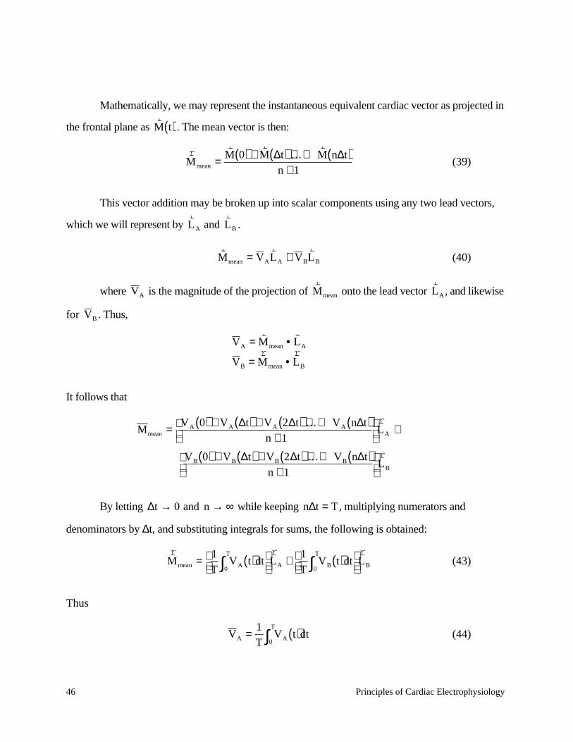
vectors. The mean electrical axis of the heart is that angle, α, that the mean vector makes with the
horizontal (see Fig. 34). Note that angles are measured clockwise clinically, starting from the
horizontal. Normal axes fall between –10˚ and +110˚.
Figure 34 — The Mean Electrical Cardiac Vector
I II III
Figure by MIT OCW.
46 Principles of Cardiac Electrophysiology
Mathematically, we may represent the instantaneous equivalent cardiac vector as projected in
the frontal plane as rM t( ). The mean vector is then:
rM mean =
rM 0( ) +
rM ∆t( ) +…+
rM n∆t( )
n +1(39)
This vector addition may be broken up into scalar components using any two lead vectors,
which we will represent by rL A and
rL B .
rM mean = VA
rL A + VB
rL B (40)
where VA is the magnitude of the projection of rM mean onto the lead vector
rL A , and likewise
for VB . Thus,
VA =rM mean•
rL A
VB =rM mean•
rL B
It follows that
Mmean = VA 0( ) + VA ∆t( ) + VA 2∆t( ) +…+ VA n∆t( )n +1
rL A +
VB 0( ) + VB ∆t( ) + VB 2∆t( ) +…+ VB n∆t( )n +1
rL B
By letting ∆t → 0 and n → ∞ while keeping n∆t = T, multiplying numerators and
denominators by ∆t, and substituting integrals for sums, the following is obtained:
rM mean = 1
TVA t( )dt
0
T
∫
rL A + 1
TVB t( )dt
0
T
∫
rL B (43)
Thus
VA = 1T
VA t( )dt0
T
∫ (44)
Principles of Cardiac Electrophysiology 47
VB = 1T
VB t( )dt0
T
∫ (45)
VA t( ) and VB t( ) are simply the scalar projections of rM on
rL A and
rL B . They are scalar functions
of time (the ECG). The time, T, is the duration of the QRS complex.
If
rM mean•
rL A = 1
TVA t( )dt
0
T
∫ = 0
then rM mean must be perpendicular to
rL A . This observation allows the clinician to make a rapid
estimate of the mean electrical axis of the heart from a quick inspection of the six frontal scalar
leads. One simply locates that lead where the mean area under the QRS complex is zero, or nearly
so, and concludes that the mean axis of the heart is perpendicular to that lead. The sense of the
vector is easily determined by observing the polarity of the net area under the curve of lead I. For
example, if this area were positive, the mean axis would have to lie in quadrants I or IV. Thus, in
Figs. 32 and 33 above, we see that since
1T
V III t( )dt0
T
∫ ≈ 0,
the mean electrical axis must be perpendicular to lead III: either +30˚ or –150˚. Since VL > 0, the
mean axis must be +30˚.
One may approximate areas under the QRS complex by measuring amplitudes only, and
assuming equal widths for positive and negative spikes. The net area is then proportional to the sum
of all positive peaks in the QRS minus the sum of all negative spikes. In this way, the ratio of any
two arbitrary means may be calculated, and the mean axis constructed graphically.