Embed Size (px)
Citation preview
NBER WORKING PAPER SERIES
CAREER TECHNICAL EDUCATION AND LABOR MARKET OUTCOMES:EVIDENCE FROM CALIFORNIA COMMUNITY COLLEGES
Ann Huff StevensMichal Kurlaender
Michel Grosz
Working Paper 21137http://www.nber.org/papers/w21137
NATIONAL BUREAU OF ECONOMIC RESEARCH1050 Massachusetts Avenue
Cambridge, MA 02138April 2015, Revised February 2018
The research reported here was supported in part by the Institute of Education Sciences, U.S. Department of Education, through Grant R305C110011 to Teachers College, Columbia University. The opinions expressed are those of the authors and do not represent views of the Institute or the U.S. Department of Education. We gratefully acknowledge the California Community Colleges Chancellor’s Office for providing us with data access, technical support, and expertise. We are also appreciative of financial support from the Center for Poverty Research at UC Davis, funded by the U.S. Department of Health and Human Services, Office of the Assistant Secretary for Planning and Analysis (ASPE), the Interdisciplinary Frontiers in the Humanities and Arts Program at UC Davis, and from the Smith Richardson Foundation. The authors are responsible for all errors. The opinions expressed are those of the authors alone and not those of agencies providing data or funding, nor of the National Bureau of Economic Research.
NBER working papers are circulated for discussion and comment purposes. They have not been peer-reviewed or been subject to the review by the NBER Board of Directors that accompanies official NBER publications.
© 2015 by Ann Huff Stevens, Michal Kurlaender, and Michel Grosz. All rights reserved. Short sections of text, not to exceed two paragraphs, may be quoted without explicit permission provided that full credit, including © notice, is given to the source.

Career Technical Education and Labor Market Outcomes: Evidence from California Community CollegesAnn Huff Stevens, Michal Kurlaender, and Michel GroszNBER Working Paper No. 21137April 2015, Revised February 2018JEL No. I24,I26
ABSTRACT
Career technical education (CTE) programs at community colleges are increasingly seen as an attractive alternative to four-year colleges, yet little systematic evidence exists on the returns to specific certificates and degrees. We estimate returns to CTE programs using administrative data from the California Community College system linked to earnings records. We employ estimation approaches including individual fixed effects and individual-specific trends, and find average returns to CTE certificate and degrees that range from 14 to 45 percent. The largest returns are for programs in the healthcare sector; estimated returns in non-health related programs range from 15 to 23 percent.
Ann Huff StevensDepartment of EconomicsOne Shields AvenueUniversity of California, DavisDavis, CA 95616and [email protected]
Michal KurlaenderUniversity of California, DavisOne Shields AvenueSchool of EducationDavis, CA [email protected]
Michel GroszUniversity of California, DavisOne Shields AvenueDepartment of EconomicsDavis, CA [email protected]
Stevens, Kurlaender, and Grosz 1
1
I. Introduction For the past half-century, the earnings of Americans with less than a four-year college
degree have stagnated or fallen. Despite widespread increases in postsecondary participation, the
fraction of Americans completing bachelor’s degrees has not risen substantially in decades, and
is declining for some groups (National Center for Education Statistics, 2016; Bailey & Dynarski,
2011; Turner, 2004). Although many efforts have focused on increasing educational attainment,
it is clear that encouraging college enrollment in traditional academic pathways is not sufficient.
Important demographic and labor market changes have demanded a more skilled workforce with
increased postsecondary training. Vocational or career technical education (CTE) programs are
often recognized as an important part of the solution to workforce training needs, but returns to
specific CTE programs have rarely been systematically or convincingly evaluated.
Many CTE programs are offered through public state community college systems. These
community colleges are the primary point of access to higher education for many Americans. In
California, the setting for this study, two-thirds of all college students attend a community
college. As the largest public community college system, one-sixth of all community college
students in the nation are enrolled at a California community college. Over the years,
California’s community colleges have grown and have been applauded for remaining affordable,
open-access institutions, but also continually criticized for producing weak outcomes, in
particular low degree receipt and low transfer rates to four-year institutions (Sengupta and
Jepsen, 2006; Shulock and Moore, 2007). Moreover, CTE programs within California’s
community colleges, which often attract students without an explicit goal to transfer to
bachelor’s-granting institutions, have often been omitted from these discussions (Shulock,
Moore, and Offenstein, 2011; Shulock and Offenstein, 2012).

Stevens, Kurlaender, and Grosz 2
2
This paper takes a major step toward filling the gap in the literature on returns to CTE
progams in higher education. Using longitudinal administrative data from the largest community
college system in the nation, we estimate the returns to specific CTE certificates and degrees. By
taking advantage of the fact that the vast majority of CTE students have substantial pre-
enrollment earnings histories, we are able to present detailed estimates of the labor market
returns to completing CTE certificates and associate degrees. We use these data to estimate
models that control for both fixed unobservable factors that may be correlated with certificate or
degree completion, and for similar factors that change at a constant rate over time. The fixed
effects approach produces estimates of the return to certificates and degrees relative to earnings
in the absence of degree receipt, using individuals’ own pre-enrollment earnings as the critical
control variables. We utilize a control group of individuals enrolling but not completing degrees
and certificates, which, in the fixed effects setting, help to identify common year, age, and
enrollment effects. Estimates based on a subset of our data that use parental background and high
school test scores to control for heterogeneity in OLS regressions produce slightly larger
estimates than our fixed effects models, confirming the importance of controlling for
unobservable, fixed factors.
Our approach also addresses the tremendous heterogeneity in types of program offerings
within the broad grouping of CTE programs, and we separately analyze fields that include a wide
range of courses preparing students for careers as police, prison officers, health care providers, or
construction workers, among others. We find returns to CTE programs that range from 14
percent (for certificates of less than 18 units) to 45 percent (for associate degrees). We find
especially large returns for programs in the health sector, ranging from 12 to 99 percent. Results
are not sensitive to our specific choices involving a control group or control variables.
Stevens, Kurlaender, and Grosz 3
3
II. Prior Research on the Returns to Postsecondary Schooling
As part of the large literature on returns to higher education, a growing number of authors
have focused on community colleges, with fewer focused on CTE programs. On the broader
topic of returns to community college enrollment and awards, for example, Belfield and Bailey
(2011) review a number of studies over the past several decades. As these authors note, the vast
majority of those studies are correlational in nature, comparing the earnings of those who do and
do not attend or complete community college programs.1 Many of these studies fail to control for
potentially important sources of bias, including ability bias, or are inattentive to more general
contamination of the estimates by correlation between degree completion or attendance and
unobserved personal characteristics. Thus, while there are many examples of studies that show
higher earnings associated with community college attendance, until recently there has been little
evidence establishing a causal connection between community college programs and earnings.
Even less such evidence exists for CTE programs within community colleges.
Kane and Rouse (1995) estimated returns to accrued credits (and degrees) at community
colleges and found returns to coursework at exclusively vocational colleges separately, but did
not separate vocational and traditional academic programs within community colleges. They
found returns to credits earned at vocational schools that were similar to or smaller than returns
to credits from two-year colleges. Bailey et al. (2004a) found that CTE associate degrees produce
larger gains than academic associate degrees, using a standard OLS framework with no controls
for ability bias or other unobservables. Leigh and Gill (1997) focused on returning adults, using
1 For examples of these observational studies comparing those with and without community college credits or degrees see Rosenbaum and Rosenbaum (2013), Belfield and Bailey (2011), or Bailey et al. (2004b).
Stevens, Kurlaender, and Grosz 4
4
an OLS framework with a rich set of control variables, and found positive returns to community
college degrees, similar to the more traditionally aged students studied by Kane and Rouse
(1995).
An important advance in this literature came from Jacobson, LaLonde, and Sullivan (JLS,
2005) who evaluated the return to CTE programs within Washington State community colleges.
Their innovation was to use both individual fixed effects and individual-specific earnings trends
to control for unobservables that are correlated with both earnings (levels and trends) and the
likelihood of completing training. Surprisingly, most studies following JLS (2005) have not
included or tested for robustness to individual-specific trends.
Beyond the methods used, the study by JLS is important for two additional reasons, both
of which relate to and motivate our study. First, these authors recognized that CTE programs
provide an opportunity for causal identification of the return to CTE that is not often available
for higher education studies more generally. The use of fixed effects and individual-specific
trends depends critically on having multiple earnings observations prior to enrollment in the
program. For students pursuing traditional academic paths, this is often impossible since they
have very limited earnings observations prior to enrolling in college. Second, JLS are among the
first to document that there may be substantial heterogeneity in returns across different programs
or disciplines in the CTE realm. They found, for example, returns of approximately 14% for men
and 30% for women in “technically oriented math and science courses” in the CTE realm, but
essentially no return for other CTE coursework. The sample for their study was notably a group
of high tenure displaced workers and therefore may not apply to the broader group of students in
CTE programs.

Stevens, Kurlaender, and Grosz 5
5
More recently, a number of studies have made use of administrative earnings data linked
to community college records to estimate returns to a community college education. These
studies have been far more inclusive of CTE programs, though not typically focusing on CTE
programs specifically. Jepsen, Troske, and Coomes (2014) estimated models with individual
fixed effects and found positive returns to both CTE associate degrees and shorter “diplomas” for
men, but less evidence of returns to diplomas for women. They did not include individual-
specific trends, but did interact observable characteristics with trends as a substitute for more
fully controlling for time-varying unobservables. They did not present estimates for specific
programs of study within the broader category of CTE. Bahr et al. (2015) followed a similar
approach using data from Michigan, and estimated returns separately for some specific CTE
awards, including shorter certificates and associate degrees. However, small sample sizes within
individual study areas limited Bahr et al. (2015) to estimate returns for a smaller set of shorter-
term CTE certificates, and those estimated often had large confidence intervals.
A pattern of heterogeneous effects across programs was also found in Dadgar and
Trimble (2016) using data from the state of Washington. They showed, surprisingly, negative
and significant effects of short-term certificates on earnings for women, and no statistically
significant returns for men, but positive significant returns of long-term certificates for women
and no significant returns to for men. Their estimates for field-specific certificates were also
limited by small samples, making it difficult to draw sharp conclusions. Finally, Xu and Trimble
(2016) showed positive and significant returns, on average, to both short- and longer-term
certificates in North Carolina and Virginia. When they disaggregated by field of study, results
were mixed, with both positive and negative statistically significant effects depending on the
field of study. Both of these studies used fixed effects models and a control group of students
Stevens, Kurlaender, and Grosz 6
6
enrolling in courses but not completing certificates or degrees. They did not, however, examine
robustness to individual-specific trends.
A final study, similar to many of those described above, is important because its
comparison of standard cross-sectional and fixed effects estimates makes clear that methodology
can make a substantive difference. Liu, Belfield, and Trimble (2015) showed that OLS estimates
with controls for ability and demographics produce negative, and sometimes significant, effects
of short-term CTE certificates. Interestingly, models including fixed effects suggested positive
and significant effects for the same programs. This pattern of results suggests negative selection
of individuals (in terms of earnings) into certificate programs. This implies that it may be very
important, particularly in the case of short-term CTE programs, to control for earnings prior to
enrollment in a flexible way.2
Finally, an unpublished study by Bahr (2016), developed simultaneously with ours, also
uses administrative data from California Community Colleges, and a fixed effects approach.
Bahr’s findings for CTE programs appear to be qualitatively similar to ours. Courses of study
and award types for which we find the largest returns also show large returns in Bahr’s work, and
similarly for many of those with smaller returns. Our work differs from Bahr’s not only in our
closer focus on CTE programs, but also in several aspects of our econometric specifications.
Notably, the fixed effects approach used in both studies requires earnings prior to enrollment to
control for individual productive ability. We make the case below that these pre-enrollment
earnings are widely available among our sample of CTE students, but may not be for more
2 Another similar, unpublished, study in this area is by Bettinger and Soliz (2016), who find positive effects of sub-baccalaureate degrees at Ohio postsecondary institutions, with important heterogeneity by gender, field of study, and certificate type. While they do use a fixed effects approach to control for selection bias, they lack pre-enrollment earnings data and must rely on earnings while enrolled in college to identify returns in a fixed effects setting. As the authors note, this could lead to biases in either direction.

Stevens, Kurlaender, and Grosz 7
7
traditional academic paths. Bahr estimates returns to all community college programs, some of
which are populated largely by traditional students entering the system straight from high school
who cannot have much earnings history to support the fixed effects approach.3 Of course, his
estimates focusing on CTE programs should not be directly affected by this concern. Bahr does
not test for the existence of differential trends among award completers and non-completers prior
to enrollment.
A related issue is that Bahr estimates a single equation with interaction terms to estimate
returns for more than 50 different awards (both CTE and traditional academic), while we allow
separate regressions for each CTE program and award length. We have replicated his approach
and find estimates to be fairly sensitive to whether we estimate a single equation or separate
equations for each award type, particularly when estimated using earnings levels rather than logs.
We suspect this may explain many of the differences between our point estimates and Bahr’s and
prefer the additional flexibility of separate equations across fields.4
The literature to date, particularly recent studies that have used pre-enrollment earnings
data to implement fixed effects estimators, has produced mixed results on the returns to CTE,
particularly for certificates and diplomas below the associate degree level. This heterogeneity in
estimated returns highlights the need for studies that can disaggregate CTE programs and
estimate returns for relatively specific programs of study. In addition, short of randomization or a
quasi-experimental design, recent studies show that it is important to have extensive pre-
3 Bahr’s Table 1, for example, shows that half of his sample is age 18 or 19 and he reports an average age at enrollment of 25 years, nearly five years lower than our average age. This difference is likely driven by the distinction between CTE students and all community college students. 4 One additional difference is that Bahr allows effects to vary by years since the award was completed using a quadratic in quarters. We have estimated models that allow effects to vary over time, but use a more flexible step function. (See Appendix Table A1).

Stevens, Kurlaender, and Grosz 8
8
enrollment earnings data and a population with substantial labor market experience before
enrollment.
Our contributions in this paper fill an important gap in this literature by combining data
from a large population of CTE programs including a variety of occupational fields and award
lengths with longitudinal data methods that make best use of these rich data. We focus
exclusively on CTE programs within the California Community College system, and the
corresponding student population with substantial work experience prior to enrollment. Unlike
some similar work, we look at the entire universe of students enrolling in CTE programs, rather
than starting from specific categories of CTE program users such as displaced workers or welfare
recipients. In addition, our access to the entire population of students in this system for 23 years
allows us to provide disaggregated estimates for a wide spectrum of CTE certificates and
degrees. Finally, we utilize our long time-series of earnings data to estimate models that control
for both individual fixed effects and individual-specific trends, as was done by Jacobson,
LaLonde, and Sullivan (2005), but not later authors. The potential importance of these controls
was recently highlighted by Dynarksi, Jacob, and Kreisman (2016) who discuss the assumption
of common earnings trends (conditional on fixed effects) across groups with different degree
outcomes, and recommend testing the robustness of earnings results to the individuals-trends
model we utilize here. This produces results that provide an estimate of the return to completing
certificates and degrees (including accumulation of all of the required units), relative to their own
prior earnings patterns, and adjusting for age, time and common shocks using data from
individuals pursuing (but not completing) the same type of degree or certificate.
Stevens, Kurlaender, and Grosz 9
9
III. Data
The California Community Colleges system consists of 114 campuses and is the largest
public higher education system in the country, enrolling over 2.6 million students annually (Scott
& Perry, 2011). The state’s large public postsecondary system of sub-baccalaureate colleges
offers great individual and institutional diversity. Colleges represent urban, suburban, and rural
regions of California, range in size from 1,000 to over 40,000 students enrolled each semester,
and offer a wide range of CTE and traditional academic programs to a diverse set of students.
CTE programs are a prominent part of the overall mission of community colleges. In a typical
year in California, more than half of all awards issued are for a CTE degree, and more than
60,000 of these CTE awards are given annually in recent years. We illustrate this in Appendix
Figure A1, which summarizes the number of CTE and total awards issued by California
community colleges for the years covered in our sample. The top line shows all awards from the
colleges for each year from 1996 to 2013, and the line immediately below shows the subset of
CTE degrees. The figure also shows that these CTE awards are distributed across the various
certificate and degree lengths described earlier.
We combine two sources of data for the analysis, tracking California community college
students through their postsecondary schooling and into the labor market between 1992 and
2011. First, we use detailed administrative records from the California Community Colleges
Chancellor’s Office (CCCCO), which include college-level and student-level information.
Specifically, we employ information on students’ demographic background, course-taking
behavior, and degree receipt by term.5 We match these data to quarterly student earnings
5 Only three colleges use the quarter system, which makes synchronizing the school year to the calendar year straightforward. For the rest, which are on the semester system, we categorize the spring semester (January to June) as the first and second quarters, with summer term and fall semester as the third and fourth quarters, respectively.
Stevens, Kurlaender, and Grosz 10
10
information from the state’s unemployment insurance (UI) system.6 These data are linked to
student information by the CCCCO and extend from 1992 to 2012. Approximately 93 percent of
students in our college data are matched to earnings records.7 Prior to 2001 there were several
changes in reporting practices and retirements within the college system and so we focus on the
college data from the later half of the period it is available.
The CCCCO data contain a vast amount of student-level information. Demographics,
such as a student’s age, race, and gender, are recorded in each academic term for which a student
was enrolled in a course. We define enrollment based on the units attempted in a given term:
part-time between six and 12 units, and full-time as more than 12 units. These two definitions are
consistent with the number of units needed to qualify for different levels of financial aid. We do
not differentiate between students taking fewer than six units and those not enrolled because the
workload of a single course is not likely to depress earnings.8
We categorize the content of different courses and programs according to the Taxonomy
of Programs (TOP), a system unique to California’s community colleges but similar to the more
commonly used Classification of Instructional Programs (CIP) codes. All community colleges in
the state are required to use the TOP, which grants us a uniform categorization of the topical
content of degrees and courses across time that is common across all of California’s community
colleges. In particular, the CCCCO identifies some TOP codes as CTE, which allows us to note
students who take such courses and earn CTE-identified degrees. In this analysis we focus on
6 We have access to these data as they are provided to the CCCCO through the California Employment Development Department (part of the California Department of Finance). 7 Students may not be observed in the earnings records for several reasons including being in an uncovered sector (including armed forces members, railroad workers, self-employed, domestic workers and unpaid family workers) over the period, a true lack of any formal earnings, or having moved out of the state with no recorded earnings in California. See http://www.labormarketinfo.edd.ca.gov/data/QCEW_About_the_Data.html for details of quarterly earnings coverage. 8 In the appendix, we show that adding a separate control for being enrolled for less than six units has no effect on earnings or on our estimated returns.
Stevens, Kurlaender, and Grosz 11
11
awards in TOP codes designated as CTE programs. The narrowest TOP code is a six-digit
number denoting a field. The first two digits identify one of 24 broad disciplines, such as
education, biological sciences, or health. There are CTE and non-CTE fields within each
discipline, though the distribution is not uniform across disciplines; for example, engineering and
industrial technologies (TOP code 09) has many more CTE fields than the social sciences (TOP
code 22).
We evaluate the effects of CTE award attainment by looking at four categories
representing a traditional sub-baccalaureate degree (associate degree) and several other short-
term certificates. Specifically, we categorize award holders into four categories: Associate of
Arts/Sciences degrees (typically 60 credit hours); 30–59 credit certificates; 18–29 credit
certificates, and 6–17 credit certificates.9 Students enrolled full-time typically take 15 units per
semester, so these various awards range from two years of full-time coursework to less than a
semester.
IV. Sample Construction
To evaluate the returns to CTE awards, we first construct a sample of students who
earned a CTE certificate or degree between 2003 and 2007. While our college-based data do
extend back into the 1990s, there were a number of changes in reporting requirements for
individual colleges during that period. This allows us to focus on a period with consistent data
reporting and quality, and primarily use the community college data from 2001 forward.10 We
begin with relatively broad categories of TOP code disciplines. We focus on the eleven largest
9 The data do not allow us to disaggregate beyond these groupings. 10 We use 2003 as the first year of student completions in order to have pre-enrollment data for all students.

Stevens, Kurlaender, and Grosz 12
12
TOP code disciplines to maintain reasonable sample sizes for our discipline-specific estimates.
Combined, these disciplines cover approximately 98 percent of all CTE degrees granted during
the period. We conduct the analyses separately by discipline. Focusing on these large disciplines
allows us to look separately at degrees within specific disciplines.
We limit the sample of treated individuals to just those students who earned a CTE
degree—though this may not have been their highest degree. We place no restrictions on the first
term of enrollment, which means some of these students may have earned their degree in just a
year while others may have taken much longer. On average students take four years to complete
their first CTE award. We match earnings data back to 1992, regardless of when students began
their coursework. For most students, the earnings data extend from before they enrolled for the
first time in a community college course until after they graduated. We limit the sample to years
of data between five years prior and ten years after a student’s first term enrolled in a community
college. We drop earnings and academic data for students in the years before they turned 18
years old. Students may take classes at multiple colleges throughout their academic careers and
they can also transfer credits from one community college to another. For the purposes of our
sample and because of certain data limitations, we consider each student at each college as an
individual case.11
While transfers to four-year universities are common among community college students
generally, they are far less common among CTE students. To avoid conflating the value of a
four-year degree with the value of completing shorter CTE programs, we drop from our sample
any individuals that our data indicate transferred to a four-year college. We examine sensitivity
11 A student who earned a degree at college X and a degree at college Y will be included in our data twice, once for his career at each college. For a student who took courses at college X and college Y, but only earned a degree at college Y, we only observe the coursework and degree earned at college Y; the coursework at college X drops out of our sample.
Stevens, Kurlaender, and Grosz 13
13
to this choice following our main results and show that, for most CTE fields, this does not alter
our conclusions.
V. Statistical Framework for Estimating Returns to CTE Programs
Our goal in this paper is to estimate credible causal effects of CTE programs on earnings,
both overall and by individual CTE disciplines. An answer to the fundamental question of
whether CTE programs produce returns comparable to traditional academic, four-year degrees is
essential in a policy environment that recommends CTE degrees as an important alternative to
traditional baccalaureate degrees. An advantage of studying CTE programs is the fact that most
CTE students do not enroll directly from high school, unlike traditional college students, and so
we can use standard identification approaches that make use of earnings prior to enrollment to
control for unobserved characteristics.
Our goal is to identify the earnings effect of completing a CTE degree relative to not
completing such a degree, or
(1) E(Yit|CTE Award=1) – E(Yit|CTE Award=0),
where Yit represents quarterly earnings. The key challenge, as in much of the literature on returns
to education, training programs, or costs of worker displacement, is that we cannot observe the
same individual in both states of the world, with and without the CTE award, at the same time.
Prior literature has used a variety of approaches to measure earnings in the absence of an award,
including those never enrolling in a program, those not completing a program, or those
completing different programs. Here we use fixed effects approaches in which earlier earnings of
individuals who eventually receive awards, adjusted for growth and economy-wide factors over
time, serve as a proxy for later earnings in the absence of the award. We include control groups

Stevens, Kurlaender, and Grosz 14
14
in order to assist with the identification of time and year dummies and improve efficiency.12 We
show below that our results are not sensitive to changes in our control group, reflecting the fact
that the thrust of our identification strategy comes from individual degree recipients’ own prior
earnings.
Given the focus on returns to degrees in the broader literature on higher education, we
view it as important to estimate returns to comparable, structured courses of study in the CTE
arena. CTE certificate and degree programs represent a focal course of study, similar to
traditional academic degrees, that are meant to prepare students for a particular occupation or set
of occupations. Moreover, although there are many other potential questions of interest, such as
whether there is a return to accumulating credits (but not necessarily a formal degree or
certificate), or how returns to CTE degrees vary across colleges, these are secondary to the
question of whether there is an average return to the degree or certificate itself. Issues of
selection into specific fields are also of substantial interest, but again are secondary to
establishing credible returns across those fields. Thus, our parameter of interest is receipt of a
CTE degree or certificate.
To answer the question of whether completion of CTE programs improves the earnings
of award receipients, we use a regression framework similar in spirit to the literature on non-
experimental evaluations of worker training programs.13 The majority of students in our sample
of those taking CTE courses have earnings prior to enrollment and many have a substantial
earnings history prior to enrollment. We construct our estimation strategy to make use of these
12 See Jacobson, Lalonde, and Sullivan (1993) for a clear discussion of similar models, including the role of the control group (in their case never displaced workers) in the estimation. 13 See, for example, Heckman, and Smith (1999), or Heckman, Lalonde, and Smith (1999).

Stevens, Kurlaender, and Grosz 15
15
pre-enrollment earnings and to better isolate the causal effect of CTE awards on earnings.
Specifically, we estimate equations of the form:
(2) ln(𝐸𝐸𝐸𝐸𝐸𝐸𝐸𝐸𝐸𝐸𝐸𝐸𝐸𝐸𝐸𝐸)𝑖𝑖𝑖𝑖 = 𝛼𝛼𝑖𝑖 + 𝛾𝛾𝑖𝑖 + 𝜃𝜃𝑖𝑖𝑡𝑡 + 𝜋𝜋𝐸𝐸𝐸𝐸𝐸𝐸𝜋𝜋𝜋𝜋𝜋𝜋𝜋𝜋𝑑𝑑𝑖𝑖𝑖𝑖 + 𝛽𝛽𝛽𝛽𝜋𝜋𝐸𝐸𝐸𝐸𝜋𝜋𝜋𝜋𝑖𝑖𝑖𝑖 +∑ 𝛿𝛿𝑗𝑗 1(𝐴𝐴𝐸𝐸𝜋𝜋 = 𝑗𝑗)𝑖𝑖𝑖𝑖65𝑗𝑗=18 +
𝜀𝜀𝑖𝑖𝑖𝑖
These regressions include individual fixed effects (αi), so that the effect of the award
receipt is identified from the within-person changes in earnings from before to after the award is
received. They also include individual-specific trends, 𝜃𝜃𝑖𝑖𝑡𝑡, to avoid bias in the estimates from
unobserved factors that may be correlated with completion and that change at a constant rate
over time. This is important since we show below that there is evidence suggesting different pre-
enrollment earnings trends between our treatment and control groups, so that a standard fixed
effects approach may not completely eliminate sources of bias. This specification reflects the
approach recommended by Dynarski, Jacob and Kreisman (2016) in their recent consideration of
whether fixed effects alone are likely to be sufficient to fully control for pre-enrollment earnings
patterns.
The specification also includes controls—in the form of dummy variables—for calendar
year and age. We enter age as a series of dummy variables (δj) to capture non-linear age effects
on earnings. The coefficient π captures the effect of an indicator for periods in which the
individual is enrolled at the community college either full- or part-time. This is to avoid
conflating part-time or otherwise reduced earnings while enrolled with pre-enrollment earnings
as a base against which this specification implicitly compares post-award earnings. The
coefficient of interest, β, takes a value of one in periods after the student has graduated.
This equation could be estimated using only degree recipients with earnings observed
both before and after the award receipt. In this approach, the dummy for “Degree” initially

Stevens, Kurlaender, and Grosz 16
16
equals zero, and then turns to one upon completion of the award. By the end of the sample
period, every individual in the treated part of our sample has completed the award.
In our main results, we also include control groups in the estimation of equation (2). Our
control groups include those taking at least eight units in the particular CTE discipline, but not
receiving a degree or certificate. They are constructed on the basis of both data availability and
the desire to best identify those individuals most similar to award recipients in particular CTE
programs. We have earnings data only for individuals who have had some contact with the
California Community College system, but that involvement can be as minimal as enrollment in
a single course. Control groups within the fixed effects approach used here serve simply to
identify the age and year effects and so better estimate the hypothetical path of earnings in the
absence of degree receipt. In Appendix Figure A2, we show the distribution of units completed
for both treatment and control groups. Control group members, as expected, complete far fewer
units than the treated group. At the same time, treatment and control group students are far more
similar in terms of demographic characteristics within disciplines than across, reflecting
differences across disciplines in the characteristics of students taking even a few classes (Table
1). As shown below, our estimates are not sensitive to using alternative control groups.
The main concern with non-experimental estimates of the effects of education on
earnings is that individuals who choose to enroll and complete degrees may be more motivated
or productive than those who take only a few courses or do not enroll at all. This could lead to a
systematic overstatement of the earnings effects of these programs. Our inclusion of individual
fixed effects and individual-specific trends should address many of these concerns. This
approach is feasible in the CTE setting because so many CTE students are involved in the labor
Stevens, Kurlaender, and Grosz 17
17
market prior to their enrollment, and our approach makes good use of this unique feature of CTE
programs.14
There remain some potential concerns and sources of bias with our specification.
Specifically, if transitory, unobserved shocks to our treated group affect both their likelihood of
completing a degree and their subsequent earnings (and are not captured by their pre-enrollment
earnings levels or growth rates), this could bias our estimated returns. This cannot be completely
addressed with the observational data available here, a caveat similar to that made by Jepsen et
al. (2014). A recent review by Belfield and Bailey (2017) highlights the challenges of using fixed
effects estimators in this setting. Our access to data with both many years of earnings and large
numbers of students allows us to overcome many of the challenges they cite, and we show below
that our results are robust to a number of specification changes. Overall, the ability to control for
pre-enrollment earnings and earnings trends, and the very large samples available from this
unique dataset, allow us to provide arguably the most convincing estimates to date of the labor
market returns to a wide variety of specific CTE programs.15
Given that we have data only on individuals who have at one point enrolled in the
community college system, our sample is necessarily conditioned on that enrollment. More
specifically, we condition on participation in at least some level of CTE coursework and so our
14 Note that this means we will be identifying off of individuals that do have a pre-enrollment earnings history. If there is heterogeneity in returns to these CTE programs across more- and less-experienced workers, our estimates based on equation (2) will predominantly represent the returns to award recipients with more prior work experience, since those without such experience will not contribute much of the within person variation we need for this identification approach. We investigate this by focusing on returns for workers of different ages and do not find evidence that this systematically changes our estimates. 15 Recent work in progress by Flaaen, Shapiro, and Sorkin (2016) makes a similar point about the effect of matching or propensity score approaches that control for observables in settings that also include fixed effects. In their work on the earnings costs of displacement (estimated with individual fixed effects), they note that reweighting procedures based on observable characteristics make little difference to their estimates. They explain this by noting that once individual fixed effects are included “reweighting only changes estimates if these characteristics predict different slopes of earnings.” In our case, the inclusion of individual-specific earnings trends would similarly address selection factors associated with different earnings slopes.

Stevens, Kurlaender, and Grosz 18
18
results are directly applicable to that portion of the population. Similarly, our earnings results
reflect the economic environment of California from 2001 to 2011, but we note that this includes
a great deal of heterogeneity across both geography and time. For example, county
unemployment rates over this time period ranged from nearly 17 percent in Fresno County in
2010 to under six percent in San Francisco during 2004.16 Moreover, the California Community
College system is the largest community college system in the country, serving one out of every
six community college students nationwide. Thus, while some concerns about external validity
and sensitivity to market conditions will always be relevant to studies based on a single state or
single system of higher education, our sample is broad and diverse along many dimensions. This,
along with our ability to control for fixed and smoothly trending unobservables, make our
estimates widely applicable.
Finally, for a subset of our sample, we utilize an alternative identification approach,
based on access to a very rich set of additional control variables that can proxy for underlying
abilities that might be correlated with the propensity to complete a CTE award. As a robustness
check, we estimate models that do not include individual fixed effects, but that control for high
school math and English language arts test scores and parental education, as well as demographic
characteristics. We expect that this approach, which controls for a fuller set of observable
characteristics, but cannot control for fixed unobserved characteristics or for trends that are
correlated with degree receipt, will lead to higher estimated returns. We also test models that
interact estimated returns with pre-enrollment test scores, but find no evidence that those with
higher test scores (a proxy for ability) have systematically different returns to completion.
16 See, http://www.labormarketinfo.edd.ca.gov/data/unemployment-and-labor-force.html, for county-level unemployment rates in California from 1990 to the present.
Stevens, Kurlaender, and Grosz 19
19
VI. Results
A. Summary Statistics
Table 1 provides detailed summary statistics for our CTE award recipients for the eleven
largest TOP codes, or CTE disciplines, and the associated comparison groups. Several points
from Table 1 inform our interpretation of the results below. First, there is tremendous
heterogeneity in student characteristics, distribution of award types, and pre-enrollment labor
market attachment across the eleven CTE disciplines. For example, just 36 percent of those
receiving awards in the area of business and management were employed just prior to their initial
enrollment, but more than half of those in health or public and protective services were employed
immediately prior to their initial enrollment. Gender differences across fields are also striking; 94
percent of those receiving awards in engineering and industrial technology were male, but only
12 percent in family and consumer sciences were male. Only one-third of award recipients in
health were male. This points out the potential importance of estimating returns to degrees
separately across discipline, since observable (and unobservable) characteristics vary
dramatically across disciplines and may have important implications for estimating and
interpreting overall returns.
The average age at enrollment in our sample ranges from a low of 21 for commercial
services to over 30 for agriculture and law, differentiating this sample from more traditional,
non-CTE college programs. Between 50 and 70 percent of students had at least one quarter of
nonzero earnings before first enrolling, and approximately 40 percent had more than five
quarters. Depending upon the field, we observe between five and 15 quarters of nonzero earnings
prior to enrollment.

Stevens, Kurlaender, and Grosz 20
20
Table 1 also provides information on how similar our treatment and control groups are to
one another. Age and gender distributions are similar across the treatment and control groups
within specific TOP codes. This is important given the large differences in these characteristics
across TOP codes and suggests the potential value of having control groups that are specific to
each discipline. One potentially important difference between the treatment and control groups is
that, across TOP codes, the control group is usually more likely to be employed prior to
enrollment. This may reflect the greater tendency of employed students to take only a few
courses, rather than completing a full degree or certificate program. Our use of individual fixed
effects should prevent this from being a major source of bias, by effectively conditioning on pre-
enrollment earnings.
Before turning to regression models, Figure 1 shows event-study graphs of the pattern of
log earnings around the time of completion of certificates and degrees. These figures come from
regressions of log earnings on a vector of quarterly event-time dummies (from 20 quarters prior
to 25 quarters post) defined for the treatment group, along with controls for calendar year, age,
and current enrollment. As in the regression models specified above, the control group
contributes to estimation of common calendar year, age and enrollment effects. We show these
results for each of the four award lengths for all TOP codes together, and for the three largest
TOP codes. Focusing on the figures for all TOP codes together, several patterns are obvious.
First, there do appear to be noticeable increases in earnings following degree receipt relative to
the period prior to completion. Second, there is some visual evidence that for several disciplines
and award types the treated group (relative to the comparison group) had negative earnings
trends prior to their enrollment and completion of degrees. These event study models, which do
not account for individual fixed effects and trends as in the main estimating equation, instead
Stevens, Kurlaender, and Grosz 21
21
serve to highlight the scope of the identification problem when not controlling for fixed effects
and trends. This makes it important to test for the presence of non-parallel trends prior to
enrollment and to check our estimates’ robustness to controlling for such trends. Finally, these
event-study graphs hint at the heterogeneity in returns we find across different fields and award
lengths. Among associate degree recipients, for example, there appear to be large returns in
health, but small or no returns in the area of business and management. In contrast, among the
shortest awards, of just six to 17 units, public and protective services seems to show larger
earnings increases after completion than health or business and management.
B. Regression Results
1. Main results
We next turn to regression results, using the specification summarized in equation (2).
Recall that our control group for each TOP code consists of students who earned at least eight
units in that discipline within their first three years of enrollment at the college, following the
CCCCO’s definition of a CTE-degree bound student.
In Table 2, we present results from our preferred regression specification by certificate or
degree length and discipline. Disciplines are listed from the largest in terms of awards granted (at
the top) to the smallest (at the bottom). First, we note that there are positive and significant
returns to most of the CTE programs studied here. Table 2 shows that, in 34 out of 44 cases,
there are positive and statistically significant earnings effects of these CTE certificate and degree
programs. For the relatively large programs, effects are estimated quite precisely so that even
some modest returns are statistically significant. For example, short certificates of under 18 units
in information technology show one of the smaller returns at approximately 10 percent, and these
Stevens, Kurlaender, and Grosz 22
22
returns are statistically different from zero.17 A second broad finding from Table 2 is that there is
a striking degree of heterogeneity in estimated returns across different TOP codes. A 30–59 unit
certificate in business, for example, produces an earnings effect of approximately 11.5 percent
(coefficient 0.109), compared to an estimated return of 17 percent (coefficient of 0.154) in public
and protective services, and nearly 49 percent in health (coefficient of 0.398).
Table 2 also shows substantial heterogeneity by program length, not always in the
expected direction. In many cases, returns do increase as the length of the program increases, but
there is not perfect monotonicity. For example, in health, estimated returns increase as the length
of the certificate program grows. In contrast, in public and protective services, the estimated
return to certificates requiring 18 to 29 units exceeds the returns for longer certificate programs
and the AA/AS degree. To some extent, this lack of monotonicity may reflect that many of the
broad TOP codes are themselves heterogeneous in terms of the types of CTE programs they
include. Public and protective services, for example, includes programs in fire protection,
administration of justice, and policing. This means that differences in program length may be
confounded with differences in the nature of the training and related occupations. Below, we
aggregate programs of different lengths and show that, on average, certificates with greater unit
requirements have higher returns, even though this may not be true within every individual TOP
code.
A different type of heterogeneity in returns to community college degrees is highlighted
in recent work by Andrews, Li, and Lovenheim (2016) who estimate quantile treatment effects
and show substantial variation in earnings of community college graduates. While their results
do not include shorter-term certificates, the heterogeneity in returns we show here across CTE
17 In the log earnings specification, the percentage effect on earnings is given by eβ – 1, where β is the reported coefficient.

Stevens, Kurlaender, and Grosz 23
23
fields is consistent with the broad range of earnings effects for community college students
shown in that work.
Several recent studies have estimated similar models using earnings levels, rather than
the log specification used here. Appendix Table A2 shows results from repeating our basic
specification on the same sample, but using earnings levels as the dependent variable. Results
based on earnings levels produce similar results, though with implied percentage effects (using
pre-enrollment earnings as a baseline) that are typically smaller than results in Table 2. Appendix
Table A3 shows estimates of similar models with the outcome being the probability of
employment (having positive earnings). Those results show small positive effects on
employment in most fields, with estimated effects typically between two and four percent. The
columns of Table A2 where we estimate the main results in earnings levels are consistent with
this finding. When we include zero earnings observations (not shown) our estimated effects on
earnings increase slightly, reflecting this additional effect of improving the chances of having
positive earnings. In general, the results using levels are similar to the log specifications in terms
of which fields have large, or very large returns. The very right-skewed distribution of quarterly
earnings leads us to prefer the log specification, which should be less sensitive to some extreme
values for earnings.
Summary statistics from Table 1 indicate large gender differences in enrollment patterns
across specific programs and disciplines. Because we also document substantial heterogeneity in
returns across disciplines, we next investigate the returns to CTE programs separately for men
and women. Table 3 shows similar returns for men and women in most disciplines. Information
technology is one exception, with certificates of 30 to 59 units showing large, marginally
significant returns for women and low or no returns for men. The reverse is true for AA/AS

Stevens, Kurlaender, and Grosz 24
24
degrees in the Information Technology area. Relatively few women receive certificates and
degrees in the information technology TOP code and so these results for women are imprecisely
estimated. Among all associate degrees awarded to women, fewer than two percent are in this
TOP code. This also raises the possibility of some gender-specific selection into fields that could
complicate interpretation of returns. Our summary from these results overall is that, although
there are some differences in returns by gender, they are small relative to gender differences in
selection into CTE fields.
To better understand this variation in returns and field choices, we have also estimated
returns separately by more detailed, four-digit TOP codes, which correspond much more closely
to well-defined fields of study or occupations. For example, rather than estimating the return to
all 18 to 29 unit certificates in the broad field of family and consumer sciences, we instead allow
separate coefficients for returns to programs in: child development/early care and education;
fashion; and interior design. These results are displayed in Figure 2, in which our estimated
returns by four-digit TOP code and program length are illustrated on the vertical axis, grouped
into the broad disciplines and program lengths we used in Table 2. The advantage of this is that it
allows us to show variation in returns across the specific programs in which students enroll. For
each discipline we also show (filled in circles) the overall return for the discipline and degree
length for comparison. Figure 2 displays the statistically significant returns for 200 different
programs. For ease of display, we omit 11 coefficients over 1.0 and 7 coefficients under -0.3;
another 195 coefficients were not statistically different from zero. A similar figure with all
estimated returns, including those not statistically different from zero, is shown in the
Appendix.18 There is substantial variation in returns to specific four-digit TOP codes around the
18 The full list of individual estimates at the four-digit TOP code level is available online at http://jhr.uwpress.org/.

Stevens, Kurlaender, and Grosz 25
25
average for the broad discipline. For example, in health the estimated coefficients range from
essentially zero for a small certificate in emergency medical services to approximately 0.20 for a
30-59 unit certificate in health information technology, to a high of 0.83 for an associate degree
in respiratory care therapy.
This variation in returns—across and within disciplines—has an obvious counterpart in
the literature on variation in returns to college by major. Altonji, Bloom, and Meghir (2012)
report returns—based on OLS estimation with detailed occupational controls—for 23 different
college majors. They show that the standard deviation of returns across these majors ranges from
0.07 for women to 0.10 for men. Our results are similar, with a standard deviation in estimated
returns across the two-digit TOP codes of 0.08 to 0.17, depending on the length of the certificate
or degree. The literature on college majors has often struggled for convincing identification of
the true returns to college majors; the results reported by Altonji, et al. (2012) likely include
some bias from unobservables that could contribute to the variation across majors. Our results
for CTE programs are among the few that are based on estimation that controls for time-invariant
unobservables.
Work by Arcidiacono (2004) looks at variation in returns across just four broad four-year
college majors and finds a span of 10 to 20 percentage points, after controlling for unobserved
heterogeneity in selection into majors, a similar span to our results if we exclude associate’s
degrees in health. Overall, our results demonstrate that, even after controlling for potential ability
differences (via the fixed effects and individual-specific trends), there is variation across CTE
fields that is roughly comparable to the extent of variation in returns across majors found for
bachelor’s degrees.
Stevens, Kurlaender, and Grosz 26
26
The heterogeneity across specific types of CTE programs may explain why studies that
consider all CTE programs can be challenging to interpret. Differences in the mix of degree
programs offered, or specific patterns of enrollment, may alter the overall estimate of returns. At
the same time it is of interest to present a tractable summary of expected returns for the
population of CTE students. One way to summarize these estimated returns is to calculate a
weighted average return where the weights take account of the relative frequency of degrees in
specific disciplines. This also allows for a way to summarize overall returns that captures
differences in enrollment patterns by gender. In Table 4, we provide this summary by calculating
weighted averages across TOP codes for each degree type.
The weights for this exercise are the fraction of all degrees of a specific type earned in
the four-digit TOP code out of all such degrees earned.19 This provides an estimate of the typical
return for a random student receiving a CTE associate degree or certificate of a given length,
with TOP codes that grant relatively large numbers of degrees receiving greater weight. Given
the very large returns to health-related occupations, we also repeat the exercise for all disciplines
other than health. This shows smaller overall returns for women than for men, particularly when
health is excluded from the estimates. Given the similarity across gender of discipline-specific
returns in Table 3, these results largely reflect differences in the specific programs completed by
men and women. For women, the returns range from approximately ten percent for certificates
requiring just six to 18 units to approximately 40 percent for the associate degree. For men, the
comparable range is 14 to 45 percent.
19 This is not the only sensible way to aggregate returns across disciplines. This approach produces an overall return to the “average” degree recipient. Another strategy might be to weight by the number of students attempting degrees in this field; this would produce an average return more appropriate to a typical potential awardee.

Stevens, Kurlaender, and Grosz 27
27
In the lower panel of Table 4 we repeat this summary of results excluding health
programs. This shows smaller, but still substantial, positive average returns for CTE programs of
all lengths outside the health sector. Overall, estimated returns outside of health range from nine
to 20 percent among women, with the largest average returns accruing to certificates requiring 30
to 59 units of study. Among men, average returns range from 14 to 26 percent, depending upon
the length of the certificate or degree. For comparison, Jepsen et al. (2014) report earnings
returns for CTE associate degrees (excluding health) of approximately $1,300 to $1,500 in
quarterly earnings, or increases of 26 to 30 percent given their baseline quarterly earnings of
approximately $5,000. Our results are in a similar range.
These results provide strong evidence of the potential of short-term CTE programs to
substantially raise earnings. Even excluding health-related occupational programs, which are
known to have substantial returns, our findings show the potential for significantly improved
earnings for students who complete these short-term CTE programs.
2. Robustness Checks
a. Robustness to individual-specific trends
Our main specification allows for individual-specific trends, an approach that has been
recommended in this literature (Jacobson, Lalonde and Sullivan, 2005; Dynarski, Jacob and
Kreisman, 2016), but that has not always been implemented. While including individual-specific
trends can potentially address concerns about bias that remains in a fixed effects setting, it can
also raise other concerns and may not effectively address bias in the presence of dynamic
treatment effects. In this section, we examine the performance and robustness of models that
control for individual-specific trends.
Stevens, Kurlaender, and Grosz 28
28
To test whether individual-specific trends in earnings are correlated with degree and
certificate completion, we follow the suggestion in Dynarski, Jacobs, and Kreisman (2016) who
recommend testing for earnings trends that are correlated with completion by estimating
regressions of pre-enrollment earnings (for treatment and control groups) that include indicators
for eventual completion interacted with a time trend. We regress log earnings prior to enrollment
on trends, and on trends interacted with a dummy equal to one for those individuals who
eventually complete a degree or certificate. Additional controls include year and quarter fixed
effects, and, in some specifications, demographic controls. When we group all TOP codes
together, our results indicate that the parallel trends assumption is violated for only one of the
four award lengths (certificates of 18 to 29 units). When we disaggregate by TOP code, however,
we find that five of the 40 coefficients that could indicate differential pre-enrollment trends are
statistically different from zero. While evidence of potential bias occurs in a minority of the
estimates, it is more than can be clearly ascribed to chance. This, along with the visual evidence
of pre-enrollment trends shown in Figure 1 supports a primary specification using individual-
specific trends.
Unfortunately, models that include controls for individual-specific or group-specific
trends can conflate the influence of pre-treatment trends with trends or dynamics in the treatment
effects (Wolfers, 2006), and as a result may not effectively correct estimates for pre-treatment
trends. One of the implications of the Wolfers (2006) argument is that individual-specific trends
should only be used if there is an a priori reason to believe they may be important. In our case, a
primary concern with estimating returns to education in a non-experimental framework is that
unobserved productive ability or skill might influence both earnings (levels and trends) and
completion probabilities, and so we view it as important to test for this possibility in our setting.
Stevens, Kurlaender, and Grosz 29
29
To consider whether the critique of Wolfers (2006) with respect to including individual-
specific trends might be applicable in our analysis, we combine the testing for differential trends
described above with tests for whether including individual-specific trends significantly alters
our estimated returns to completion, and a careful examination of the direction of any resulting
changes. Seven of the 44 coefficients from Table 2 are significantly changed (using a generous
ten percent significance level) when we drop the individual-specific trends.
To understand these two sets of test results, we combine them in Table 5, which shows
results of tests for differential pre-enrollment trends (column one) and for equality of our key
coefficients with and without controls for individual-specific trends (columns two through four).
Note that Table 5 does not include all TOP codes, but rather only those six TOP codes for which
there were either statistically significant differential pre-earnings trends for award recipients or
evidence suggesting rejection of equality of coefficients with and without individual-specific
trends. (The remaining TOP codes did not meet these conditions.)
Among the five awards for which there were significantly different pre-enrollment trends,
as indicated by stars in column 1, one award produces results in which the trends specification
moves the coefficients of interest in a direction consistent with the sign of the pre-enrollment
trends. The remaining four cases produce results in which including trends does not significantly
alter the key coefficient, and are split with two cases moving point estimates in the expected
direction and two not.
Among awards in the health TOP code, there is evidence that eventual award recipients
have more negative earnings trends prior to enrollment. Table 5 also shows that conditioning on
individual-specific trends leads to larger estimated returns, consistent with a reduction in bias
Stevens, Kurlaender, and Grosz 30
30
from controlling for more negative pre-enrollment trends among those who eventually complete
awards.
In contrast, within public and protective services, we find evidence that controlling for
individual-specific trends may not control well for potential bias. Table 5 shows that including
trends does not move the estimates in the expected direction. Here, our testing provides evidence
that pre-enrollment trends for certificates of 30 to 59 units are significantly more negative among
eventual award completers. We would thus expect that controlling for individual-specific trends
should produce larger estimated returns; but we find the opposite, with the coefficient falling
from 0.19 to 0.15 in the trends specification, although this difference is not statistically
significant. Given that the only statistically significant changes in coefficients move in the
expected direction (for health awards) we prefer the specification that includes trends, but
confirm Wolfers’ (2006) note of caution concerning this specification.
We have also considered the possibility of dynamic treatment effects, which may
confound the pre-enrollment trends, by allowing the effect of award completion to vary with
time since the degree was granted. These results, summarized in Appendix Table A1, show fairly
stable treatment effects over time for many awards and do not substantially change our
conclusions regarding the specifications with and without individual-specific trends. There is
evidence that returns to awards in some TOP codes grow with time since the award, but
relatively little evidence of returns shrinking substantially over time.
b. Comparisons with OLS and detailed observable controls
An alternative to the fixed effects approach that is the basis for our estimates is a cross-
sectional, OLS, approach that includes detailed controls for observable heterogeneity in ability or
Stevens, Kurlaender, and Grosz 31
31
preparation. Even if this does not solve all of the omitted variables concerns, the frequency with
which such approaches have appeared in this literature make it useful to compare with our main
results. Importantly, for a subset of our data (certain entry cohorts), we have access to test scores
from students’ high school years, and to their parents’ completed levels of education, observable
indicators that are likely to be powerful predictors of future academic success. These results are
summarized in Table 6. We estimate OLS models for earnings, including the additional controls
for test scores and parental income, as well as fixed effects models, for the individual TOP codes
shown throughout. We then summarize the resulting coefficients using the same weighted
average approach shown in Table 4.
As expected, most of the estimated returns based on the fixed effects specification are
smaller than the OLS estimates with controls for test scores and parental education. In most
cases, however, these differences are relatively small, often within a standard error of the fixed
effects estimate. Given the much smaller samples sizes available for this exercise, we do not
draw strong conclusions here. We note that this is consistent with a role for unobserved fixed
characteristics and trends, and confirms the strong evidence that CTE programs significantly
increase earnings, even when returns are estimated in a rigorous way that controls for
unobservable factors that are either time-invariant or trend smoothly over time. Recent work by
Andrews, Li, and Lovenheim (2016) uses a similar approach, based on OLS regression with very
detailed controls. We have similar controls for family background, and pre-college ability in the
results in Table 6. Our results suggest that detailed individual observables may leave room for
bias from unobservables that are well-addressed, when feasible, with longitudinal data methods.
c. Robustness checks on main fixed effects and individual trends approach
Stevens, Kurlaender, and Grosz 32
32
We have also estimated our main specification using two alternative samples. For
convenience, column 1 of Appendix Tables A4 through A7 repeat our main specification. Our
reliance on panel data (fixed effects) methods raises a concern that we are identifying effects that
will be relevant only to older workers with substantial earnings histories. To help gauge the
likely magnitude of this concern, in the second column of these tables we show results for those
over age 30 at first enrollment. In most cases, our results for the full sample and the sample of
those age 30 and over at time of enrollment are similar. Thus, there is little evidence here to
suggest that our main estimates are less relevant for younger CTE students.
A second robustness check examines our initial choice to eliminate students who
eventually transfer to a four year institution. In work focusing specifically on CTE degree and
certificate programs, the role of transfers in driving returns is ambiguous. On the one hand,
students focused on these CTE awards may be less inclined to transfer, and so there may be less
concern that the CTE awards are associated with higher earnings partially because they facilitate
additional degrees or college attendance. This should mean that eliminating students who
transfer would reduce our estimated returns. On the other hand, transfers could work in a very
different way if academic and CTE tracks are viewed as substitutes for one another. Suppose that
individuals take a few CTE courses and thus qualify as a member of our control group; if many
of these students then decide instead to pursue a transfer path, the earnings of our controls may
benefit disproportionately from their decisions to transfer to four-year colleges. In some sense,
receiving a CTE degree could signal that a student has not opted for a four-year degree. This is
related to the “diversion” effect of community colleges in which attendance diverts students from
a four-year degree (see Belfield and Bailey, 2011 for a review and discussion). For CTE
programs, there may be an additional issue of diverting students from non-CTE programs that
Stevens, Kurlaender, and Grosz 33
33
are intended to lead to transfers. If this story is important for our CTE students, we might expect
that eliminating students who successfully transfer would disproportionately eliminate high
earning control-group members and thus increase our estimated returns.
In column 3 of Appendix Tables A4-A7, we add to the overall sample those students who
transfer. Depending on the discipline, between 12 and 40 percent of CTE students transfer to a
four-year college. These results including students who eventually transfer are very similar to
those shown in column 1, suggesting that transfers do not play a major or systematic role in
generating the returns estimated here. One exception to this pattern is for associate degrees in
Business/Management. Including those who transfer produces smaller returns to associate
degrees in Business (as well as a few other fields to a lesser degree). Business programs may be
a particularly heterogeneous group on this dimension, since many four-year colleges offer
business degrees, but they are also listed as part of the CTE offerings within the California
community colleges we study. There are both transfer-focused paths within business and specific
two-year CTE degrees that do not lend themselves to transfers. These results suggest that
focusing on those students who do not transfer provides a better estimate of the effects of the
CTE programs aimed at producing shorter-term awards.
We have also estimated models that test our decision to control only for enrollment of
more than six academic units. In Column 4, when we add a control for enrollment in one to five
units into the log wage equation, there is virtually no change in our estimates.
In the final columns of Tables A4-A7, we show how varying our control group definition
affects the estimated returns. In the final columns we show that results are not sensitive to
restricting our control group to be from approximately the same cohorts as the treated group
(first enrolling in years 2001 through 2005). We have also estimated models with a single control
Stevens, Kurlaender, and Grosz 34
34
group, consisting of students taking eight units of any CTE field, and models with no control
group. Neither of these extreme changes to the controls groups alters our estimates in a
systematic way, reflecting that individuals’ own pre-enrollment earnings supply the key
component of our identification approach.
Finally, while not shown in the tables, we conduct one other exercise to test to the
stability and robustness of our main results. This exercise is motivated by the possibility of
heterogeneous returns to CTE programs. As discussed earlier, a potentially important limitation
on the generalizability of our results is that we only observe the effect of these CTE awards for
the population that successfully complete them. If returns are systematically higher for those
with particular observed or unobserved characteristics (including those actually completing),
these results may not represent the true return for a randomly selected student. To partially
address this concern, we have also estimated models that allow for an interaction between the
effect of completion and the test scores used for the analysis in Table 6. If these test scores
provide a proxy for ability, it is important to know whether higher ability students also show
higher returns to degree receipt. All interactions between test scores and degree receipt are small
and statistically insignificant, providing little evidence that returns differ systematically across
students of different academic abilities.
VII. Discussion and Conclusion
Career technical training has been touted by many as one of the few concrete pathways to
improved earnings for those without a four-year college degree (Hoffman and Reindl, 2011;
Bosworth, 2010; Holzer & Nightingale, 2009; Harmon and MacAllum, 2003). The effectiveness
of these programs in raising earnings, however, has not been convincingly established. For-profit

Stevens, Kurlaender, and Grosz 35
35
competitors in the CTE space are frequent targets of negative press; the few evaluations we have
of CTE within public-sector community colleges have produced mixed results and have
frequently been hampered by methodological shortcoming and small samples. The potential of
CTE to improve labor market outcomes is highlighted in recent state reform efforts to strengthen
CTE offerings in California, and in recent federal funding initiatives directed at CTE and
community colleges. Research on the CTE mission of community colleges, the diverse needs of
their students, and on the relationship between CTE program offerings and the labor market has
been scarce (Rosenbaum, 2001; Grubb, 1996).
The approach used here suggests quite substantial, and generally statistically significant,
returns to a wide variety of CTE certificates and degrees offered in California community
colleges. By controlling for both individual fixed effects and individual-specific trends, we
address many concerns about using observational data to estimate returns to higher education.
Our results suggest average returns of up to 45 percent for associate degrees to approximately 14
percent for shorter-term certificates. Health programs, as expected, produce very large returns,
but other fields also result in substantial earnings gains. Excluding health leads to returns to the
associate degree and certificates of between 15 and 23 percent. While we do not perform a cost-
benefit analysis, California Community Colleges charge tuition of less than $600 per semester
for full-time study, and offer many low-income students waivers of these fees, strongly
suggesting positive net returns for students who complete awards.20
For the purpose of improving human capital development of less skilled workers, these
results raise several important points. While the returns estimated here are generally positive and
substantial, that does not mean that CTE programs are necessarily an easy solution for all
20 For information on the tuition waiver program and fee information for the system, see http://web.peralta.edu/financial-aid/sample-page/bog/, for example.
Stevens, Kurlaender, and Grosz 36
36
students or all workers. First, there is substantial heterogeneity in returns to different CTE
programs. Echoing the literature on college majors, the returns to awards with the same number
of credit hours vary enormously. While some health fields have very high returns for relatively
short programs, other certificate programs offer returns that are mere fractions of those high
returns. Even within broad disciplines (two-digit TOP codes) there is substantial variation across
specific programs. Second, there is substantial heterogeneity in the observed (and likely
unobserved) characteristics of students across disciplines and programs. Thus, sensible policies
cannot simply funnel workers into “high-return” programs, since underlying differences in the
types of students who enroll in them could be quite important. In particular, the question of how
students choose their courses of study and how redirecting students to other fields can alter their
returns remain underexplored areas.
Third, understanding the interactions between individuals, programs, and returns, in order
to provide concise information to potential students and college administrators, should be a top
priority of workforce development policies. Students should be made aware of the likely returns
on investments they are making (Klor de Alva and Schneider, 2013). College leaders should,
similarly, be aware of which programs and associated investments offer students the greatest
return on earnings. Calls to provide better information on labor market returns have begun to be
common in the broader realm of education policy, but in the CTE area, given the direct
connection to labor market outcomes, this information is especially critical.
Finding effective paths to human capital development for individuals who are unlikely to
complete standard four-year academic programs is vital. In California and the nation, declining
real wages and record high unemployment for those without college degrees, combined with cuts
to many state programs serving these populations, make it essential to understand what programs

Stevens, Kurlaender, and Grosz 37
37
can be most effective. A large literature in economics has considered the most appropriate
methods for evaluating worker-training programs, and we draw on the lessons from that
literature in this analysis.21 Short of a randomized assignment of workers into CTE courses or
programs, our approach—combining longitudinal data with a control group—provides the most
common approach in the recent literature.22 While these results cannot be generalized to every
community college system or every CTE learning environment, they do provide the first detailed
evidence for a broad group of CTE students that many programs produce substantial earnings
gains. Our results show that, even after accounting for individual pre-enrollment earnings levels
and trends, and patterns of economy-wide earnings growth, CTE programs raise earnings for
students who complete them.
21 See Card, Luve, & Weber (2010) or Lalonde (1986) for a review and meta-analysis of the job training evaluation literature, respectively. 22 Card, Luve, and Weber (2010) report that more than half of the qualifying evaluation studies included in their meta-analysis, published since 1990, used longitudinal data with a comparison group.
Stevens, Kurlaender, and Grosz 38
38
References Altonji, J.G., Blom, E. & Meghir, C. (2012). "Heterogeneity in Human Capital Investments:
High School Curriculum, College Major, and Careers," Annual Review of Economics, Annual Reviews, vol. 4(1), pages 185-223, 07.
Andrews, R.J., Li, J. and Lovenheim, M.F., 2016. Quantile Treatment Effects of College Quality on Earnings. Journal of Human Resources, 51(1), pp.200-238.
Arcidiacono, P., 2004. Ability sorting and the returns to college major. Journal of Econometrics, 121(1), pp.343-375.
Bahr, P. R. (2016). The labor market return in earnings to community college credits and credentials in California (Working Paper). Ann Arbor, MI: University of Michigan, Center for the Study of Higher and Postsecondary Education.
Bahr, P.R., Dynarski, S., Jacob, B., et al. (2015). Labor market returns to community college awards: Evidence from Michigan. (A CAPSEE Working Paper). New York, NY: Center for Analysis of Postsecondary Education and Employment.
Bailey, T., Kienzl, G. S., & Marcotte, D. (2004a). Who benefits from postsecondary occupational education? Findings from the 1980s and 1990s (CCRC Brief No. 23). Retrieved from Community College Research Center website: http://ccrc.tc.columbia.edu/publications/return-to-sub-baccalaureate-education.html
Bailey, T., Kienzl, G., & Marcotte, D. (2004b). The return to a sub-baccalaureate education: The effects of schooling, credentials, and program of study on economic outcomes. New York, NY: Columbia University, Teachers College, Community College Research Center.
Bettinger, E. & Soliz, A. (2016). Returns to Vocational Credentials: Evidence from Ohio’s Community and Technical Colleges. A CAPSEE Working Paper. New York, NY: Center for Analysis of Postsecondary Education and Employment. Available at: www.capseecenter.org
Belfield, C. R., & Bailey, T. (2011). The benefits of attending community college: A review of the evidence. Community College Review, 39, 46–68.
Belfield, C. R., & Bailey, T. (2017). Model Specifications for Estimating Labor Market Returns to Associate Degrees: How Robust Are Fixed Effects Estimates? A CAPSEE Working Paper. New York, NY: Center for Analysis of Postsecondary Education and Employment. Available at: www.capseecenter.org
Belfield, C., Liu, Y., & Trimble, M. J. (2015). The medium-term labor-market returns to community college awards: Evidence from North Carolina. A CAPSEE Working Paper. New York, NY: Center for Analysis of Postsecondary Education and Employment. Available at: www.capseecenter.org
Bosworth, B. (2010). Certificates count: An analysis of sub-baccalaureate certificates. Retrieved from Complete College America website: http://www.completecollege.org/resources_and_reports/
Card, D., Luve, J., & Weber, A. (2010). Active labour market policy evaluations: A meta-analysis. Economic Journal, 120(548), F452–F477.

Stevens, Kurlaender, and Grosz 39
39
Dadgar, M., & Trimble, M. J. (2016). Labor market returns to sub-baccalaureate credentials: How much does a community college degree or certificate pay? Education Evaluation and Policy Analysis. 37(4): 399-418
Dynarksi, S., Jacob, B. and Kreisman, D. (2016). The Fixed-Effects model in Returns to Schooling and Its Application to Community Colleges: A Methodological note. Working Paper, Center for Analysis of Postsecondary Education and Employment.
Flaaen, A., Shapiro, M, and Sorkin, I. (2016). Reconsidering the Consequences of Worker Displacements: Firm versus Worker Perspective. Working Paper. http://www.aaronflaaen.com/uploads/3/1/2/4/31243277/measuringworkerdisplacements.pdf
Grubb, W. N. (1996b). Working in the middle: Strengthening education and training for the mid-skilled labor force. San Francisco, CA: Jossey-Bass.
Harmon, R., & MacAllum, K. (2003). Documented characteristics of labor market-responsive community colleges and a review of supporting literature. Washington DC: U.S. Department of Education, Office of Vocational and Adult Education.
Heckman, J., Lalonde, R., & Smith, J. (1999). The economics and econometrics of active labor market programs. In O. Ashenfelter & D. Card (Eds.), Handbook of labor economics: Volume 3a (pp. 1865–2085). New York, NY: Elsevier
Heckman J., & Smith, J., (1999). The pre-programme earnings dip and the determinants of participation in a social programme: Implications for simple programme evaluation strategies. Economic Journal, 109(457), 313–348.
Hoffman, L., & Reindl, T. (2011). Improving postsecondary attainment among adults. Washington, DC: National Governors Association.
Holzer, H. J., & Nightingale, D. S. (2009). Strong students, strong workers: Models for student success through workforce development and community college partnerships. Washington, DC: Center for American Progress.
Jacobson, L., LaLonde, R. J., & Sullivan, D. (2005). The impact of community college retraining on older displaced workers: Should we teach old dogs new tricks? Industrial and Labor Relations Review, 58(3), 398–415.
Jepsen, C., Troske, K., & Coomes, P. (2014). The labor-market returns to community college degrees, diplomas, and certificates. Journal of Labor Economics, 32(1), 95–121.
Kane, T., & Rouse, C. (1995) Labor market returns to two- and four-year college. American Economic Review, 85(3), 600.
Klor de Alva, J., & Schneider, M. (2013). What’s the value of an associate’s degree? The return on investment for graduates and taxpayers. Washington, DC: Nexus Research and Policy Center and American Institutes for Research.
Lalonde, R. (1986). Evaluating the econometric evaluations of training programs with experimental data. American Economic Review, 76(4), 604–620.
Leigh, D. E., & Gill, A. M. (1997). Labor market returns to community colleges: Evidence for returning adults. Journal of Human Resources, 32(2), 334–353.

Stevens, Kurlaender, and Grosz 40
40
National Center for Education Statistics. Status and Trends in the Education of Racial and Ethnic Groups 2016 (NCES 2016-007). U.S. Department of Education, Washington, DC.
Rosenbaum, J. E. (2001). Beyond college for all: Career paths for the forgotten half. New York, NY: Russell Sage Foundation.
Rosenbaum, J. E., & Rosenbaum, J. (2013). Beyond BA blinders: Lessons from occupational colleges and certificate programs for nontraditional students. Journal of Economic Perspectives, 27(2), 153–172.
Scott, J., & Perry, P. (2011). Focus on results: Accountability reporting for the California Community Colleges (A Report to the Legislature). Retrieved from http://californiacommunitycolleges.cccco.edu/Portals/0/reportsTB/March_ARCC_2011.pdf
Sengupta, R., & Jepsen, C. (2006). California’s community college students (California Counts: Population Trends and Profiles, Vol. 8, No. 2). San Francisco, CA: Public Policy Institute of California.
Shulock, N., & Moore, C. (2007). Rules of the game: How state policy creates barriers to degree completion and impedes student success in the California Community Colleges. Sacramento, CA: Institute for Higher Education and Leadership.
Shulock, N., Moore, C., & Offenstein, J. (2011). The road less traveled: Realizing the potential of career technical education in the California Community Colleges. Sacramento, CA: Institute for Higher Education Leadership & Policy.
Shulock, N., & Offenstein, J. (2012). Career opportunities: Career technical education and the college completion agenda, Part 1: Structure and funding of career technical education in the California Community Colleges. Sacramento, CA: Institute for Higher Education and Leadership.
Turner, S. (2004). Going to College and Finishing College: Explaining Different Educational Outcomes, in College Choices: The Economics of Where to Go, When to Go, and How to Pay for It, Hoxby, C. (Editor). Chicago, IL: The University of Chicago Press.
Wolfers, Justin. (2006). "Did Unilateral Divorce Laws Raise Divorce Rates? A Reconciliation and New Results."American Economic Review, 96(5): 1802-1820
Xu, D., & Trimble, M. (2016). What about certificates? Evidence on the labor market returns to non-degree community college awards in two states. Educational Evaluation and Policy Analysis, 38(2):272-292.
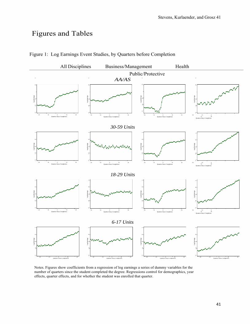
Stevens, Kurlaender, and Grosz 41
41
Figures and Tables
Figure 1: Log Earnings Event Studies, by Quarters before Completion
All Disciplines Business/Management Health Public/Protective
AA/AS
−20 −10 0 10 20 Quarters Since Completion
−20 −10 0 10 20 Quarters Since Completion
−20 −10 0 10 20 Quarters Since Completion
−20 −10 0 10 20
Quarters Since Completion
30-59 Units
−20 −10 0 10 20 Quarters Since Completion
−20 −10 0 10 20 Quarters Since Completion
−20 −10 0 10 20 Quarters Since Completion
−20 −10 0 10 20
Quarters Since Completion
18-29 Units
−20 −10 0 10 20 Quarters Since Completion
−20 −10 0 10 20 Quarters Since Completion
−20 −10 0 10 20 Quarters Since Completion
−20 −10 0 10 20
Quarters Since Completion
6-17 Units
−20 −10 0 10 20 −20 −10 0 10 20 −20 −10 0 10 20 −20 −10 0 10 20 Quarters Since Completion Quarters Since Completion Quarters Since Completion Quarters Since Completion
Notes. Figures show coefficients from a regression of log earnings a series of dummy variables for the number of quarters since the student completed the degree. Regressions control for demographics, year effects, quarter effects, and for whether the student was enrolled that quarter.
Log
Earn
ings
−.
5 0
Log
Earn
ings
0
Log
Earn
ings
0
Log
Earn
ings
0
−1
.5
1 −1
−.
5 .5
1
−1
−.5
.5
1 −1
−.
5 .5
1
Log
Earn
ings
−.
5 0
Log
Earn
ings
0
Log
Earn
ings
0
Log
Earn
ings
0
−1
.5
1 −1
−.
5 .5
1
−1
−.5
.5
1 −1
−.
5 .5
1
Log
Earn
ings
−.
5 0
Log
Earn
ings
0
Log
Earn
ings
0
Log
Earn
ings
−.
5 0
−1
.5
1 −1
−.
5 .5
1
−1
−.5
.5
1 −1
.5
1
Log
Earn
ings
−.
5 0
Log
Earn
ings
0
Log
Earn
ings
0
Log
Earn
ings
−.
5 0
−1
.5
1 −1
−.
5 .5
1
−1
−.5
.5
1 −1
.5
1

Stevens, Kurlaender, and Grosz 42
42
Figure 2: Estimates by Award Type, by Subfield and Broad Disciplines
Notes. Gray symbols show coefficients at the subfield level. Black filled-in symbols show coefficients at the larger discipline level. Only coefficients statistically significant at 95% level are shown, for a total of 200 coefficients. There are 11 coefficients over 1.0 dropped, as well as 7 coefficients under -0.3.
Estim
ated
Coe
ffici
ent
.25
.5
.75
Estim
ated
Coe
ffici
ent
0
.
25
.5
.75
−.
25
0 1
−.25
1
Arts
H
ealth
IT
Pub/
Prot
.
Com
m.
Bus.
Ag/R
es.
Fam
/Con
s.
Law
Eng/
Ind.
M
edia
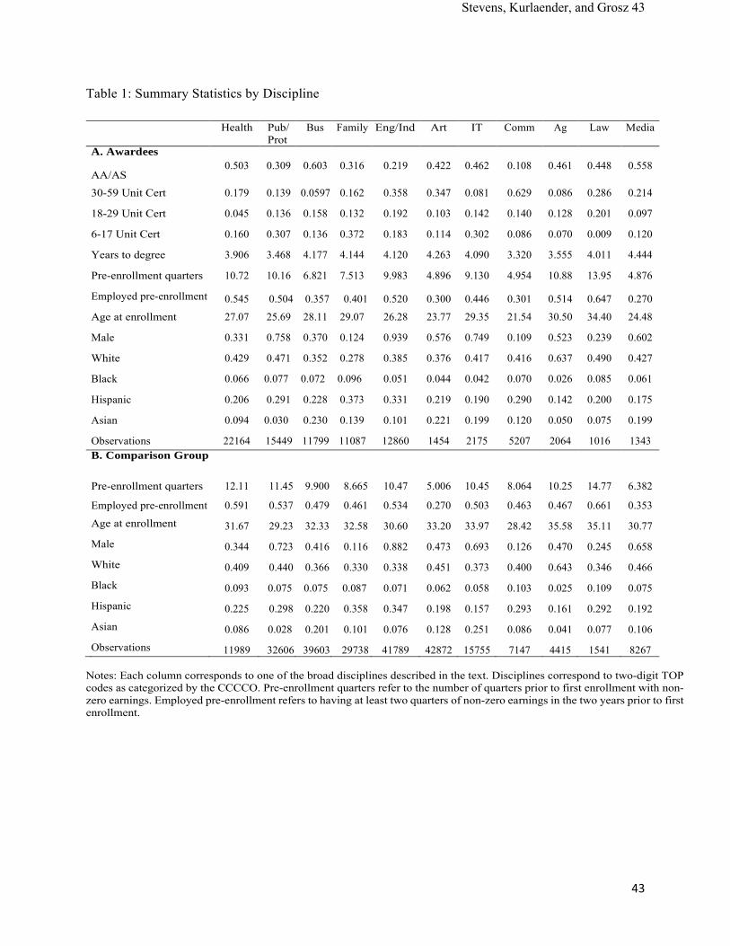
Stevens, Kurlaender, and Grosz 43
43
Table 1: Summary Statistics by Discipline
Health Pub/ Prot
Bus Family Eng/Ind Art IT Comm Ag Law Media
A. Awardees AA/AS
0.503
0.309
0.603
0.316
0.219
0.422
0.462
0.108
0.461
0.448
0.558
30-59 Unit Cert 0.179 0.139 0.0597 0.162 0.358 0.347 0.081 0.629 0.086 0.286 0.214 18-29 Unit Cert 0.045 0.136 0.158 0.132 0.192 0.103 0.142 0.140 0.128 0.201 0.097 6-17 Unit Cert 0.160 0.307 0.136 0.372 0.183 0.114 0.302 0.086 0.070 0.009 0.120 Years to degree 3.906 3.468 4.177 4.144 4.120 4.263 4.090 3.320 3.555 4.011 4.444 Pre-enrollment quarters 10.72 10.16 6.821 7.513 9.983 4.896 9.130 4.954 10.88 13.95 4.876 Employed pre-enrollment 0.545 0.504 0.357 0.401 0.520 0.300 0.446 0.301 0.514 0.647 0.270 Age at enrollment 27.07 25.69 28.11 29.07 26.28 23.77 29.35 21.54 30.50 34.40 24.48 Male 0.331 0.758 0.370 0.124 0.939 0.576 0.749 0.109 0.523 0.239 0.602 White 0.429 0.471 0.352 0.278 0.385 0.376 0.417 0.416 0.637 0.490 0.427 Black 0.066 0.077 0.072 0.096 0.051 0.044 0.042 0.070 0.026 0.085 0.061 Hispanic 0.206 0.291 0.228 0.373 0.331 0.219 0.190 0.290 0.142 0.200 0.175 Asian 0.094 0.030 0.230 0.139 0.101 0.221 0.199 0.120 0.050 0.075 0.199 Observations 22164 15449 11799 11087 12860 1454 2175 5207 2064 1016 1343 B. Comparison Group
Pre-enrollment quarters 12.11 11.45 9.900 8.665 10.47 5.006 10.45 8.064 10.25 14.77 6.382
Employed pre-enrollment 0.591 0.537 0.479 0.461 0.534 0.270 0.503 0.463 0.467 0.661 0.353
Age at enrollment 31.67 29.23 32.33 32.58 30.60 33.20 33.97 28.42 35.58 35.11 30.77 Male 0.344 0.723 0.416 0.116 0.882 0.473 0.693 0.126 0.470 0.245 0.658 White 0.409 0.440 0.366 0.330 0.338 0.451 0.373 0.400 0.643 0.346 0.466 Black 0.093 0.075 0.075 0.087 0.071 0.062 0.058 0.103 0.025 0.109 0.075 Hispanic 0.225 0.298 0.220 0.358 0.347 0.198 0.157 0.293 0.161 0.292 0.192 Asian 0.086 0.028 0.201 0.101 0.076 0.128 0.251 0.086 0.041 0.077 0.106 Observations 11989 32606 39603 29738 41789 42872 15755 7147 4415 1541 8267
Notes: Each column corresponds to one of the broad disciplines described in the text. Disciplines correspond to two-digit TOP codes as categorized by the CCCCO. Pre-enrollment quarters refer to the number of quarters prior to first enrollment with non-zero earnings. Employed pre-enrollment refers to having at least two quarters of non-zero earnings in the two years prior to first enrollment.
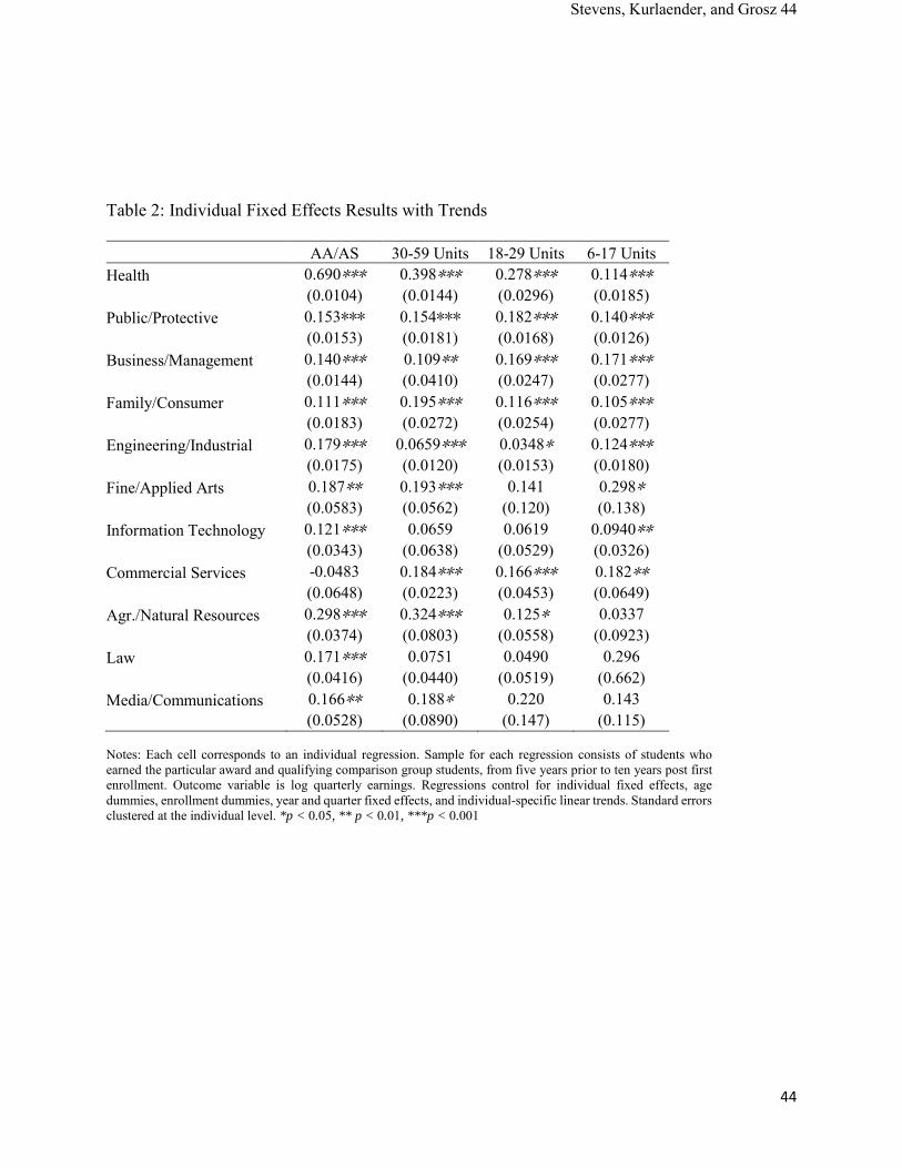
Stevens, Kurlaender, and Grosz 44
44
Table 2: Individual Fixed Effects Results with Trends
AA/AS 30-59 Units 18-29 Units 6-17 Units Health 0.690∗∗∗ 0.398∗∗∗ 0.278∗∗∗ 0.114∗∗∗ (0.0104) (0.0144) (0.0296) (0.0185) Public/Protective 0.153∗∗∗ 0.154∗∗∗ 0.182∗∗∗ 0.140∗∗∗ (0.0153) (0.0181) (0.0168) (0.0126) Business/Management 0.140∗∗∗ 0.109∗∗ 0.169∗∗∗ 0.171∗∗∗ (0.0144) (0.0410) (0.0247) (0.0277) Family/Consumer 0.111∗∗∗ 0.195∗∗∗ 0.116∗∗∗ 0.105∗∗∗ (0.0183) (0.0272) (0.0254) (0.0277) Engineering/Industrial 0.179∗∗∗ 0.0659∗∗∗ 0.0348∗ 0.124∗∗∗ (0.0175) (0.0120) (0.0153) (0.0180) Fine/Applied Arts 0.187∗∗ 0.193∗∗∗ 0.141 0.298∗ (0.0583) (0.0562) (0.120) (0.138) Information Technology 0.121∗∗∗ 0.0659 0.0619 0.0940∗∗ (0.0343) (0.0638) (0.0529) (0.0326) Commercial Services -0.0483 0.184∗∗∗ 0.166∗∗∗ 0.182∗∗ (0.0648) (0.0223) (0.0453) (0.0649) Agr./Natural Resources 0.298∗∗∗ 0.324∗∗∗ 0.125∗ 0.0337 (0.0374) (0.0803) (0.0558) (0.0923) Law 0.171∗∗∗ 0.0751 0.0490 0.296 (0.0416) (0.0440) (0.0519) (0.662) Media/Communications 0.166∗∗ 0.188∗ 0.220 0.143 (0.0528) (0.0890) (0.147) (0.115)
Notes: Each cell corresponds to an individual regression. Sample for each regression consists of students who earned the particular award and qualifying comparison group students, from five years prior to ten years post first enrollment. Outcome variable is log quarterly earnings. Regressions control for individual fixed effects, age dummies, enrollment dummies, year and quarter fixed effects, and individual-specific linear trends. Standard errors clustered at the individual level. *p < 0.05, ** p < 0.01, ***p < 0.001
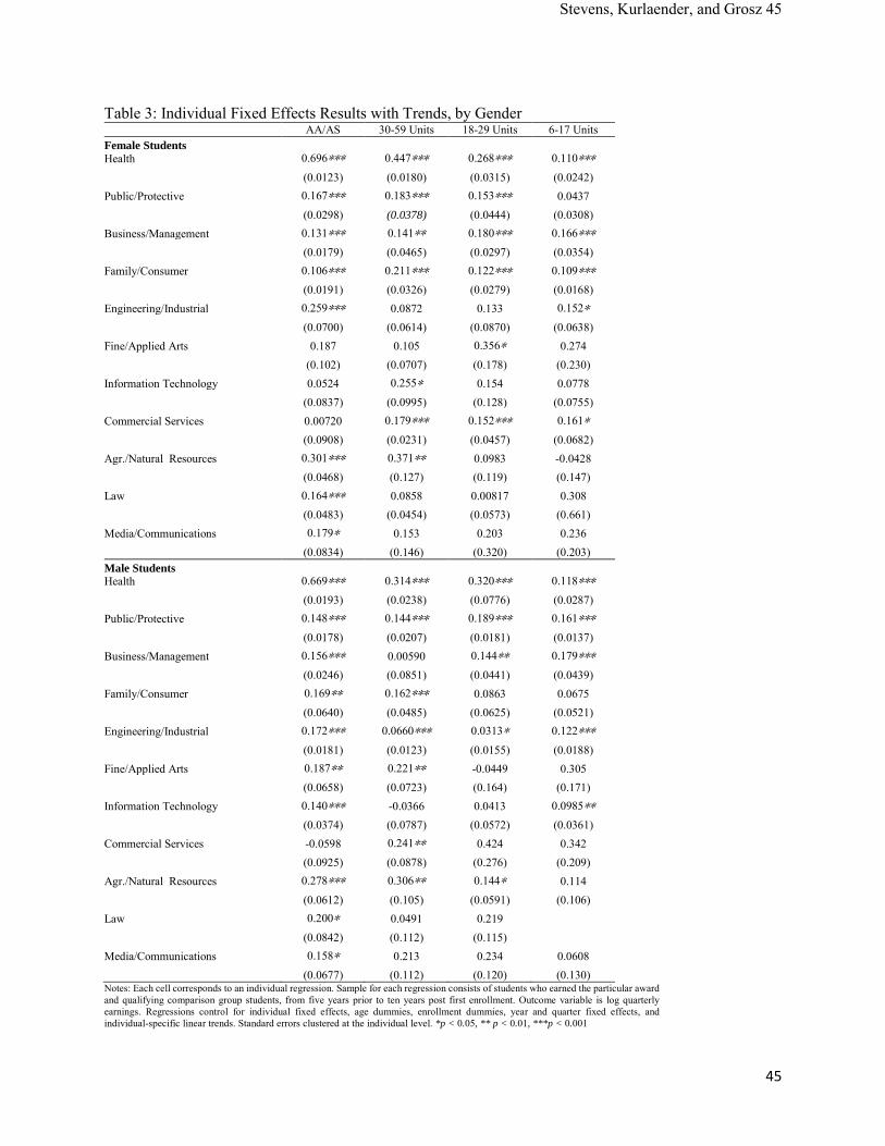
Stevens, Kurlaender, and Grosz 45
45
Table 3: Individual Fixed Effects Results with Trends, by Gender AA/AS 30-59 Units 18-29 Units 6-17 Units Female Students Health
0.696∗∗∗
0.447∗∗∗
0.268∗∗∗
0.110∗∗∗
(0.0123) (0.0180) (0.0315) (0.0242) Public/Protective 0.167∗∗∗ 0.183∗∗∗ 0.153∗∗∗ 0.0437 (0.0298) (0.0378) (0.0444) (0.0308) Business/Management 0.131∗∗∗ 0.141∗∗ 0.180∗∗∗ 0.166∗∗∗ (0.0179) (0.0465) (0.0297) (0.0354) Family/Consumer 0.106∗∗∗ 0.211∗∗∗ 0.122∗∗∗ 0.109∗∗∗ (0.0191) (0.0326) (0.0279) (0.0168) Engineering/Industrial 0.259∗∗∗ 0.0872 0.133 0.152∗
(0.0700) (0.0614) (0.0870) (0.0638) Fine/Applied Arts 0.187 0.105 0.356∗ 0.274 (0.102) (0.0707) (0.178) (0.230) Information Technology 0.0524 0.255∗ 0.154 0.0778 (0.0837) (0.0995) (0.128) (0.0755) Commercial Services 0.00720 0.179∗∗∗ 0.152∗∗∗ 0.161∗
(0.0908) (0.0231) (0.0457) (0.0682) Agr./Natural Resources 0.301∗∗∗ 0.371∗∗ 0.0983 -0.0428 (0.0468) (0.127) (0.119) (0.147) Law 0.164∗∗∗ 0.0858 0.00817 0.308 (0.0483) (0.0454) (0.0573) (0.661) Media/Communications 0.179∗ 0.153 0.203 0.236 (0.0834) (0.146) (0.320) (0.203) Male Students Health 0.669∗∗∗
0.314∗∗∗
0.320∗∗∗
0.118∗∗∗
(0.0193) (0.0238) (0.0776) (0.0287) Public/Protective 0.148∗∗∗ 0.144∗∗∗ 0.189∗∗∗ 0.161∗∗∗
(0.0178) (0.0207) (0.0181) (0.0137) Business/Management 0.156∗∗∗ 0.00590 0.144∗∗ 0.179∗∗∗
(0.0246) (0.0851) (0.0441) (0.0439) Family/Consumer 0.169∗∗ 0.162∗∗∗ 0.0863 0.0675 (0.0640) (0.0485) (0.0625) (0.0521) Engineering/Industrial 0.172∗∗∗ 0.0660∗∗∗ 0.0313∗ 0.122∗∗∗
(0.0181) (0.0123) (0.0155) (0.0188) Fine/Applied Arts 0.187∗∗ 0.221∗∗ -0.0449 0.305 (0.0658) (0.0723) (0.164) (0.171) Information Technology 0.140∗∗∗ -0.0366 0.0413 0.0985∗∗ (0.0374) (0.0787) (0.0572) (0.0361) Commercial Services -0.0598 0.241∗∗ 0.424 0.342 (0.0925) (0.0878) (0.276) (0.209) Agr./Natural Resources 0.278∗∗∗ 0.306∗∗ 0.144∗ 0.114 (0.0612) (0.105) (0.0591) (0.106) Law 0.200∗ 0.0491 0.219 (0.0842) (0.112) (0.115) Media/Communications 0.158∗ 0.213 0.234 0.0608 (0.0677) (0.112) (0.120) (0.130) Notes: Each cell corresponds to an individual regression. Sample for each regression consists of students who earned the particular award and qualifying comparison group students, from five years prior to ten years post first enrollment. Outcome variable is log quarterly earnings. Regressions control for individual fixed effects, age dummies, enrollment dummies, year and quarter fixed effects, and individual-specific linear trends. Standard errors clustered at the individual level. *p < 0.05, ** p < 0.01, ***p < 0.001
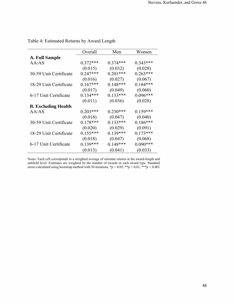
Stevens, Kurlaender, and Grosz 46
46
Table 4: Estimated Returns by Award Length
Overall Men Women A. Full Sample AA/AS 0.372*** 0.374*** 0.343*** (0.015) (0.032) (0.028) 30-59 Unit Certificate 0.247*** 0.201*** 0.263*** (0.016) (0.027) (0.067) 18-29 Unit Certificate 0.167*** 0.148*** 0.184*** (0.017) (0.049) (0.060) 6-17 Unit Certificate 0.134*** 0.133*** 0.096*** (0.011) (0.036) (0.028) B. Excluding Health AA/AS 0.203*** 0.230*** 0.159*** (0.018) (0.047) (0.040) 30-59 Unit Certificate 0.178*** 0.133*** 0.186*** (0.020) (0.029) (0.091) 18-29 Unit Certificate 0.155*** 0.139*** 0.173*** (0.018) (0.047) (0.068) 6-17 Unit Certificate 0.139*** 0.148*** 0.090*** (0.013) (0.041) (0.033) Notes: Each cell corresponds to a weighted average of estimate returns at the award-length and subfield level. Estimates are weighted by the number of awards in each award type. Standard errors calculated using bootstrap method with 50 iterations. *p < 0.05, **p < 0.01, ***p < 0.001
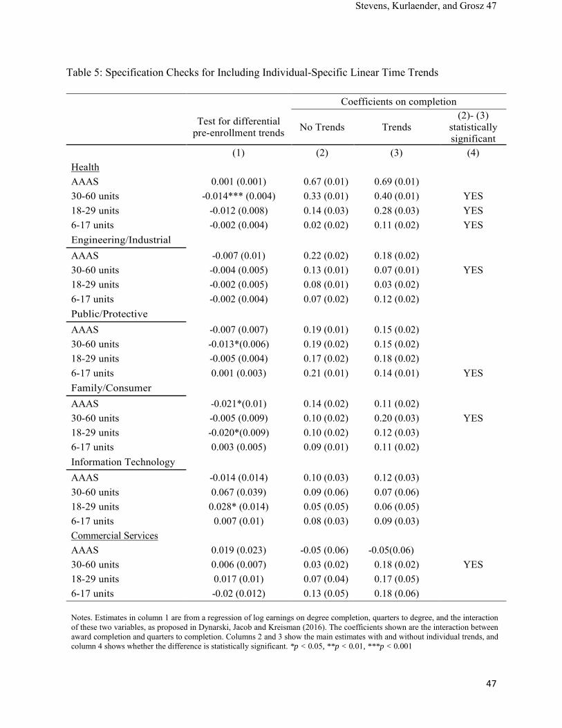
Stevens, Kurlaender, and Grosz 47
47
Table 5: Specification Checks for Including Individual-Specific Linear Time Trends
Coefficients on completion
Test for differential pre-enrollment trends No Trends Trends
(2)- (3) statistically significant
(1) (2) (3) (4) Health
AAAS 0.001 (0.001) 0.67 (0.01) 0.69 (0.01)
30-60 units -0.014*** (0.004) 0.33 (0.01) 0.40 (0.01) YES 18-29 units -0.012 (0.008) 0.14 (0.03) 0.28 (0.03) YES 6-17 units -0.002 (0.004) 0.02 (0.02) 0.11 (0.02) YES Engineering/Industrial
AAAS -0.007 (0.01) 0.22 (0.02) 0.18 (0.02)
30-60 units -0.004 (0.005) 0.13 (0.01) 0.07 (0.01) YES 18-29 units -0.002 (0.005) 0.08 (0.01) 0.03 (0.02)
6-17 units -0.002 (0.004) 0.07 (0.02) 0.12 (0.02)
Public/Protective
AAAS -0.007 (0.007) 0.19 (0.01) 0.15 (0.02)
30-60 units -0.013*(0.006) 0.19 (0.02) 0.15 (0.02)
18-29 units -0.005 (0.004) 0.17 (0.02) 0.18 (0.02)
6-17 units 0.001 (0.003) 0.21 (0.01) 0.14 (0.01) YES Family/Consumer
AAAS -0.021*(0.01) 0.14 (0.02) 0.11 (0.02)
30-60 units -0.005 (0.009) 0.10 (0.02) 0.20 (0.03) YES 18-29 units -0.020*(0.009) 0.10 (0.02) 0.12 (0.03)
6-17 units 0.003 (0.005) 0.09 (0.01) 0.11 (0.02)
Information Technology
AAAS -0.014 (0.014) 0.10 (0.03) 0.12 (0.03)
30-60 units 0.067 (0.039) 0.09 (0.06) 0.07 (0.06)
18-29 units 0.028* (0.014) 0.05 (0.05) 0.06 (0.05)
6-17 units 0.007 (0.01) 0.08 (0.03) 0.09 (0.03)
Commercial Services
AAAS 0.019 (0.023) -0.05 (0.06) -0.05(0.06)
30-60 units 0.006 (0.007) 0.03 (0.02) 0.18 (0.02) YES 18-29 units 0.017 (0.01) 0.07 (0.04) 0.17 (0.05)
6-17 units -0.02 (0.012) 0.13 (0.05) 0.18 (0.06)
Notes. Estimates in column 1 are from a regression of log earnings on degree completion, quarters to degree, and the interaction of these two variables, as proposed in Dynarski, Jacob and Kreisman (2016). The coefficients shown are the interaction between award completion and quarters to completion. Columns 2 and 3 show the main estimates with and without individual trends, and column 4 shows whether the difference is statistically significant. *p < 0.05, **p < 0.01, ***p < 0.001
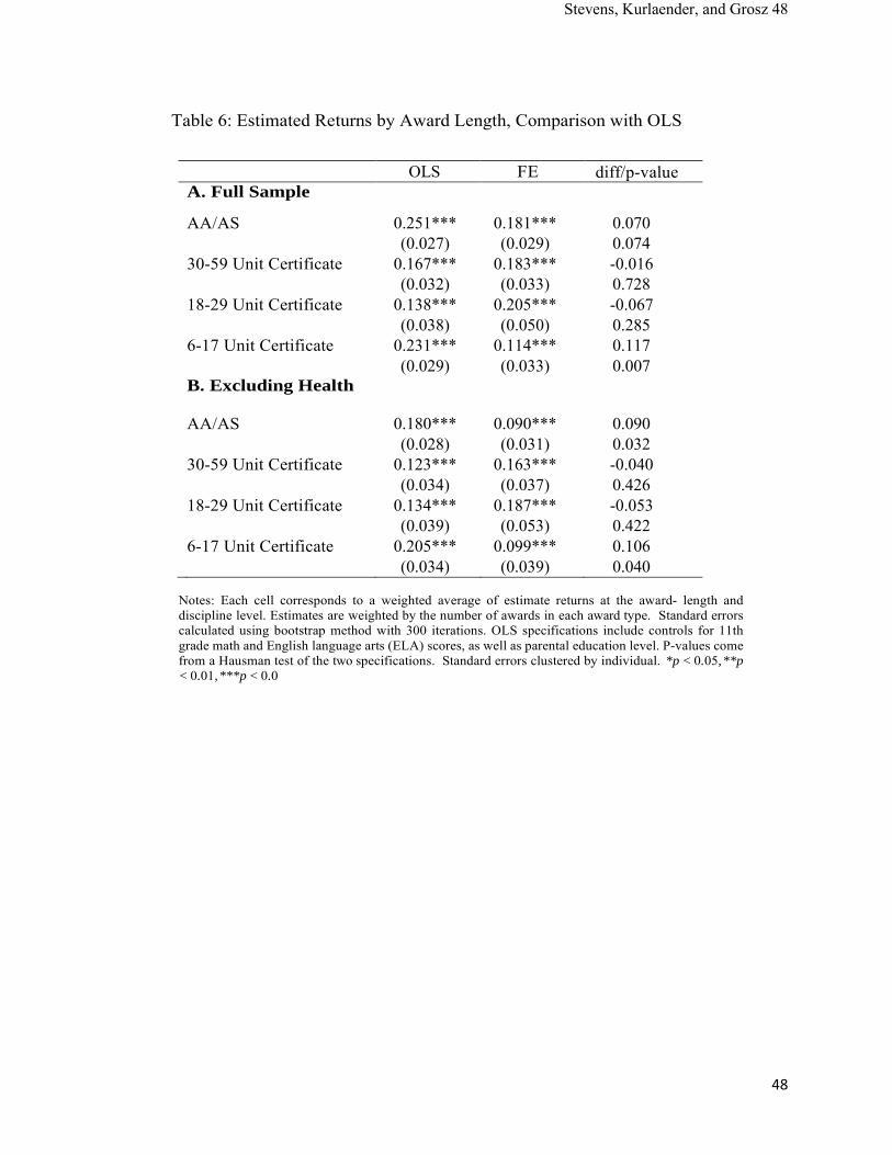
Stevens, Kurlaender, and Grosz 48
48
Table 6: Estimated Returns by Award Length, Comparison with OLS
OLS FE diff/p-value A. Full Sample AA/AS 0.251*** 0.181*** 0.070 (0.027) (0.029) 0.074 30-59 Unit Certificate 0.167*** 0.183*** -0.016 (0.032) (0.033) 0.728 18-29 Unit Certificate 0.138*** 0.205*** -0.067 (0.038) (0.050) 0.285 6-17 Unit Certificate 0.231*** 0.114*** 0.117 (0.029) (0.033) 0.007 B. Excluding Health
AA/AS 0.180*** 0.090*** 0.090 (0.028) (0.031) 0.032 30-59 Unit Certificate 0.123*** 0.163*** -0.040 (0.034) (0.037) 0.426 18-29 Unit Certificate 0.134*** 0.187*** -0.053 (0.039) (0.053) 0.422 6-17 Unit Certificate 0.205*** 0.099*** 0.106 (0.034) (0.039) 0.040 Notes: Each cell corresponds to a weighted average of estimate returns at the award- length and discipline level. Estimates are weighted by the number of awards in each award type. Standard errors calculated using bootstrap method with 300 iterations. OLS specifications include controls for 11th grade math and English language arts (ELA) scores, as well as parental education level. P-values come from a Hausman test of the two specifications. Standard errors clustered by individual. *p < 0.05, ** p < 0.01, ***p < 0.0
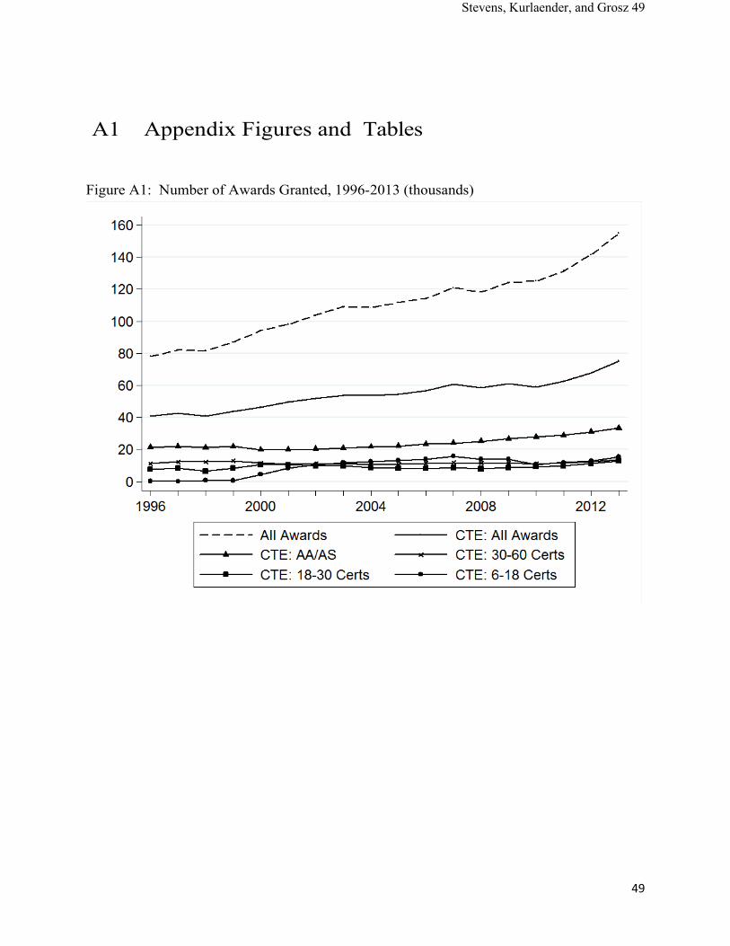
Stevens, Kurlaender, and Grosz 49
49
A1 Appendix Figures and Tables
Figure A1: Number of Awards Granted, 1996-2013 (thousands)
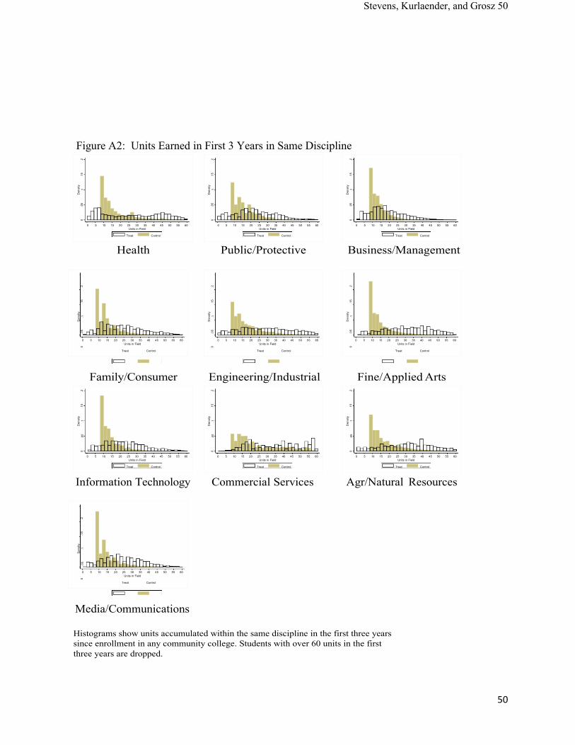
Stevens, Kurlaender, and Grosz 50
50
Den
sity
.0
5 .1
D
ensi
ty
.05
.1
Den
sity
.1
D
ensi
ty
.1
0 .1
5 .2
0
.15
.2
0 .0
5 .1
5 .2
0
.05
.15
.2
Den
sity
.0
5 .1
D
ensi
ty
.1
Den
sity
.1
0
.15
.2
0 .0
5 .1
5 .2
0
.05
.15
.2
Den
sity
.0
5 .1
D
ensi
ty
.1
Den
sity
.1
0
.15
.2
0 .0
5 .1
5 .2
0
.05
.15
.2
Figure A2: Units Earned in First 3 Years in Same Discipline
Health Public/Protective Business/Management
Family/Consumer Engineering/Industrial Fine/Applied Arts
Information Technology Commercial Services Agr/Natural Resources
Media/Communications
Histograms show units accumulated within the same discipline in the first three years since enrollment in any community college. Students with over 60 units in the first three years are dropped.
0 5 10 15 20 25 30 35 40 45 50 55 60
Units in Field
Treat Control
0 5 10 15 20 25 30 35 40 45 50 55 60
Units in Field
Treat Control
0 5 10 15 20 25 30 35 40 45 50 55 60
Units in Field
Treat Control
0 5 10 15 20 25 30 35 40 45 50 55 60
Units in Field
Treat Control
0 5 10 15 20 25 30 35 40 45 50 55 60
Units in Field
Treat Control
0 5 10 15 20 25 30 35 40 45 50 55 60
Units in Field
Treat Control
0 5 10 15 20 25 30 35 40 45 50 55 60
Units in Field
Treat Control
0 5 10 15 20 25 30 35 40 45 50 55 60
Units in Field
Treat Control
0 5 10 15 20 25 30 35 40 45 50 55 60
Units in Field
Treat Control
0 5 10 15 20 25 30 35 40 45 50 55 60
Units in Field
Treat Control
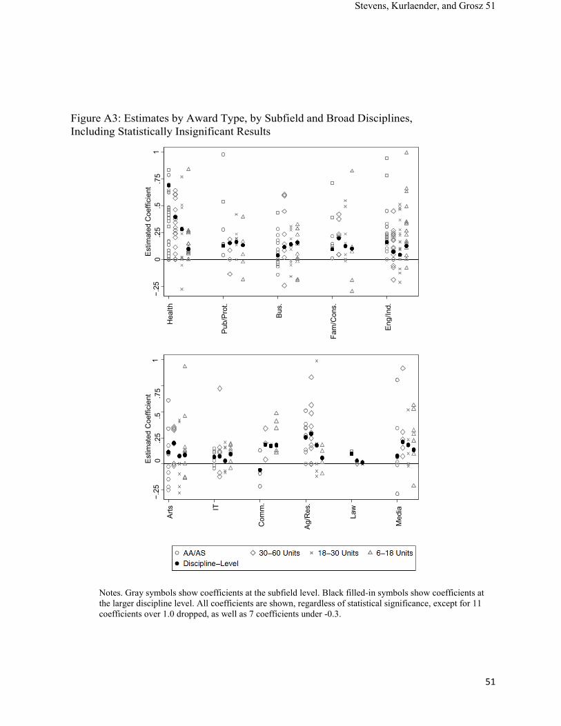
Stevens, Kurlaender, and Grosz 51
51
Figure A3: Estimates by Award Type, by Subfield and Broad Disciplines, Including Statistically Insignificant Results
Notes. Gray symbols show coefficients at the subfield level. Black filled-in symbols show coefficients at the larger discipline level. All coefficients are shown, regardless of statistical significance, except for 11 coefficients over 1.0 dropped, as well as 7 coefficients under -0.3.
Estim
ated
Coe
ffici
ent
0 .2
5 .5
.7
5 Es
timat
ed C
oeffi
cien
t 0
.25
.5
.75
−.25
1
−.25
1
Arts
H
ealth
IT
Pub/
Prot
.
Com
m.
Bus.
Ag/R
es.
Fam
/Con
s.
Law
Eng/
Ind.
M
edia

Stevens, Kurlaender, and Grosz 52
52
Table A1: Specifications with Dynamic Treatment Effects, Selected Disciplines
Trends Without Trends AA/AS 30-59 Units 18-29 Units 6-17 Units AA/AS 30-59 Units 18-29 Units 6-17 Units A. Health Main Results
Post-Completion 0.690∗∗∗
0.398∗∗∗
0.278∗∗∗
0.114∗∗∗
0.667∗∗∗
0.334∗∗∗
0.140∗∗∗
0.0241
(0.0104) (0.0144) (0.0296) (0.0185) (0.010) (0.0132) (0.0277) (0.0166) Step Function
Years 0-1 0.617∗∗∗
0.359∗∗∗
0.244∗∗∗
0.119∗∗∗
0.668∗∗∗
0.361∗∗∗
0.180∗∗∗
0.0171
(0.00961) (0.0138) (0.0278) (0.0170) (0.010) (0.0128) (0.0264) (0.0164) Years 2-3 0.607∗∗∗ 0.300∗∗∗ 0.240∗∗∗ 0.171∗∗∗ 0.666∗∗∗ 0.295∗∗∗ 0.120∗∗∗ 0.0339 (0.0147) (0.0213) (0.0418) (0.0261) (0.0134) (0.0171) (0.0331) (0.0203) Years 4+ 0.620∗∗∗ 0.280∗∗∗ 0.216∗∗∗ 0.217∗∗∗ 0.635∗∗∗ 0.240∗∗∗ -0.00725 0.0319 (0.0230) (0.0314) (0.0608) (0.0370) (0.0203) (0.0238) (0.0535) (0.0273) F-Test of Equality 1.139 9.229 0.231 6.058 2.543 19.82 8.233 0.604 p-value of Test 0.320 0.000 0.793 0.002 0.0787 0.000 0.000 0.547
B. Public/Protective Main Results
Post-Completion 0.153∗∗∗
0.154∗∗∗
0.182∗∗∗
0.140∗∗∗
0.188∗∗∗
0.186∗∗∗
0.171∗∗∗
0.209∗∗∗
(0.0153) (0.0181) (0.0168) (0.0126) (0.0139) (0.0162) (0.0159) (0.0121) Step Function
Years 0-1 0.156∗∗∗
0.150∗∗∗
0.164∗∗∗
0.128∗∗∗
0.145∗∗∗
0.172∗∗∗
0.166∗∗∗
0.201∗∗∗
(0.0143) (0.0172) (0.0165) (0.0125) (0.0133) (0.0162) (0.0160) (0.0117) Years 2-3 0.257∗∗∗ 0.169∗∗∗ 0.141∗∗∗ 0.0880∗∗∗ 0.277∗∗∗ 0.199∗∗∗ 0.172∗∗∗ 0.219∗∗∗ (0.0248) (0.0270) (0.0249) (0.0191) (0.0201) (0.0206) (0.0190) (0.0141) Years 4+ 0.328∗∗∗ 0.206∗∗∗ 0.121∗∗∗ 0.0870∗∗ 0.337∗∗∗ 0.217∗∗∗ 0.187∗∗∗ 0.217∗∗∗ (0.0393) (0.0386) (0.0350) (0.0272) (0.0327) (0.0250) (0.0218) (0.0189) F-Test of Equality 18.50 1.784 1.352 6.462 36.68 2.261 0.612 1.665 p-value of Test 0.000 0.168 0.259 0.002 0.000 0.104 0.542 0.189
C. Business Main Results
Post-Completion 0.140∗∗∗
0.109∗∗
0.169∗∗∗
0.171∗∗∗
0.139∗∗∗
0.134∗∗∗
0.199∗∗∗
0.0891∗∗∗
(0.0144) (0.0410) (0.0247) (0.0277) (0.0134) (0.0389) (0.0219) (0.0235) Step Function
Years 0-1 0.117∗∗∗
0.0917∗
0.154∗∗∗
0.154∗∗∗
0.124∗∗∗
0.103∗∗
0.153∗∗∗
0.0789∗∗∗
(0.0123) (0.0363) (0.0218) (0.0239) (0.0128) (0.0368) (0.0214) (0.0233) Years 2-3 0.117∗∗∗ 0.0978 0.206∗∗∗ 0.167∗∗∗ 0.175∗∗∗ 0.181∗∗∗ 0.255∗∗∗ 0.101∗∗∗ (0.0207) (0.0587) (0.0321) (0.0376) (0.0195) (0.0519) (0.0279) (0.0301) Years 4+ 0.100∗∗ 0.0664 0.230∗∗∗ 0.199∗∗∗ 0.180∗∗∗ 0.209∗∗ 0.316∗∗∗ 0.108∗ (0.0337) (0.0926) (0.0478) (0.0527) (0.0348) (0.0771) (0.0385) (0.0436) F-Test of Equality 0.208 0.114 3.394 0.525 5.349 2.359 15.19 0.452 p-value of Test 0.812 0.892 0.0336 0.592 0.005 0.0945 0.000 0.636
The “main results” correspond to a regression of log earnings on an individual fixed effect, controls for enrollment, and year and age effects. The “step functions” display estimates of the coefficient on three dummy variables for elapsed time since degree or certificate completion, with the omitted category being pre-completion quarters. Standard errors clustered at the individual level. ∗p < 0.05, ∗ ∗ p < 0.01, ∗ ∗ ∗p < 0.001
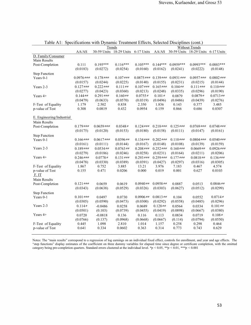
Stevens, Kurlaender, and Grosz 53
53
Table A1: Specifications with Dynamic Treatment Effects, Selected Disciplines (cont.)
Trends Without Trends AA/AS 30-59 Units 18-29 Units 6-17 Units AA/AS 30-59 Units 18-29 Units 6-17 Units D. Family/Consumer Main Results Post-Completion
0.111 0.195*** 0.116*** 0.105*** 0.144*** 0.0959*** 0.0993*** 0.0883***
(0.0183) (0.0272) (0.0254) (0.0160) (0.0162) (0.0241) (0.0222) (0.0148) Step Function Years 0-1
0.0976∗∗∗
0.178∗∗∗
0.107∗∗∗
0.0875∗∗∗
0.139∗∗∗
0.0931∗∗∗
0.0957∗∗∗
0.0802∗∗∗
(0.0157) (0.0244) (0.0225) (0.0140) (0.0155) (0.0231) (0.0215) (0.0144) Years 2-3 0.127∗∗∗ 0.222∗∗∗ 0.111∗∗ 0.107∗∗∗ 0.165∗∗∗ 0.104∗∗ 0.111∗∗∗ 0.110∗∗∗ (0.0277) (0.0423) (0.0360) (0.0213) (0.0248) (0.0335) (0.0296) (0.0190) Years 4+ 0.144∗∗ 0.291∗∗∗ 0.160∗∗ 0.0755∗ 0.101∗ 0.0879 0.0879∗ 0.0713∗∗ (0.0479) (0.0633) (0.0570) (0.0319) (0.0496) (0.0486) (0.0439) (0.0276) F-Test of Equality 1.179 2.502 0.838 2.350 1.836 0.143 0.377 3.485
p-value of Test 0.308 0.0819 0.432 0.0954 0.159 0.866 0.686 0.0307
E. Engineering/Industrial Main Results Post-Completion
0.179∗∗∗
0.0659∗∗∗
0.0348∗
0.124∗∗∗
0.218∗∗∗
0.125∗∗∗
0.0769∗∗∗
0.0748∗∗∗
(0.0175) (0.0120) (0.0153) (0.0180) (0.0158) (0.0111) (0.0147) (0.0161)
Step Function Years 0-1
0.166∗∗∗
0.0617∗∗∗
0.0396∗∗
0.134∗∗∗
0.202∗∗∗
0.110∗∗∗
0.0804∗∗∗
0.0540∗∗∗
(0.0161) (0.0111) (0.0144) (0.0167) (0.0148) (0.0108) (0.0139) (0.0159) Years 2-3 0.189∗∗∗ 0.0534∗∗ 0.0763∗∗ 0.208∗∗∗ 0.252∗∗∗ 0.160∗∗∗ 0.0669∗∗ 0.0926∗∗∗ (0.0279) (0.0186) (0.0246) (0.0258) (0.0231) (0.0164) (0.0211) (0.0206) Years 4+ 0.246∗∗∗ 0.0778∗ 0.131∗∗∗ 0.293∗∗∗ 0.259∗∗∗ 0.177∗∗∗ 0.0818∗∗ 0.136∗∗∗ (0.0478) (0.0330) (0.0389) (0.0391) (0.0427) (0.0297) (0.0316) (0.0305) F-Test of Equality 1.867 0.752 3.885 13.21 3.976 7.183 0.467 4.574 p-value of Test 0.155 0.471 0.0206 0.000 0.019 0.001 0.627 0.0103 F. IT
Main Results Post-Completion
0.121∗∗∗
0.0659
0.0619
0.0940∗∗
0.0958∗∗
0.0887
0.0513
0.0846∗∗
(0.0343) (0.0638) (0.0529) (0.0326) (0.0303) (0.0627) (0.0512) (0.0299)
Step Function Years 0-1
0.101∗∗∗
0.0497
0.0730
0.0906∗∗
0.0813∗∗
0.104
0.0552
0.0714∗
(0.0305) (0.0590) (0.0473) (0.0300) (0.0292) (0.0558) (0.0485) (0.0296) Years 2-3 0.114∗ -0.0486 0.0258 0.0689 0.128∗∗ 0.0564 0.0334 0.101∗∗ (0.0501) (0.103) (0.0739) (0.0455) (0.0419) (0.0898) (0.0667) (0.0380) Years 4+ 0.0720 -0.0818 0.136 0.116 0.113 0.0834 0.0719 0.108∗ (0.0766) (0.137) (0.0968) (0.0668) (0.0667) (0.114) (0.0794) (0.0550) F-Test of Equality 0.445 1.098 2.810 1.014 1.157 0.258 0.298 0.464 p-value of Test 0.641 0.334 0.0602 0.363 0.314 0.773 0.743 0.629
Notes: The “main results” correspond to a regression of log earnings on an individual fixed effect, controls for enrollment, and year and age effects. The “step functions” display estimates of the coefficient on three dummy variables for elapsed time since degree or certificate completion, with the omitted category being pre-completion quarters. Standard errors clustered at the individual level. *p < 0.05, **p < 0.01, ***p < 0.001
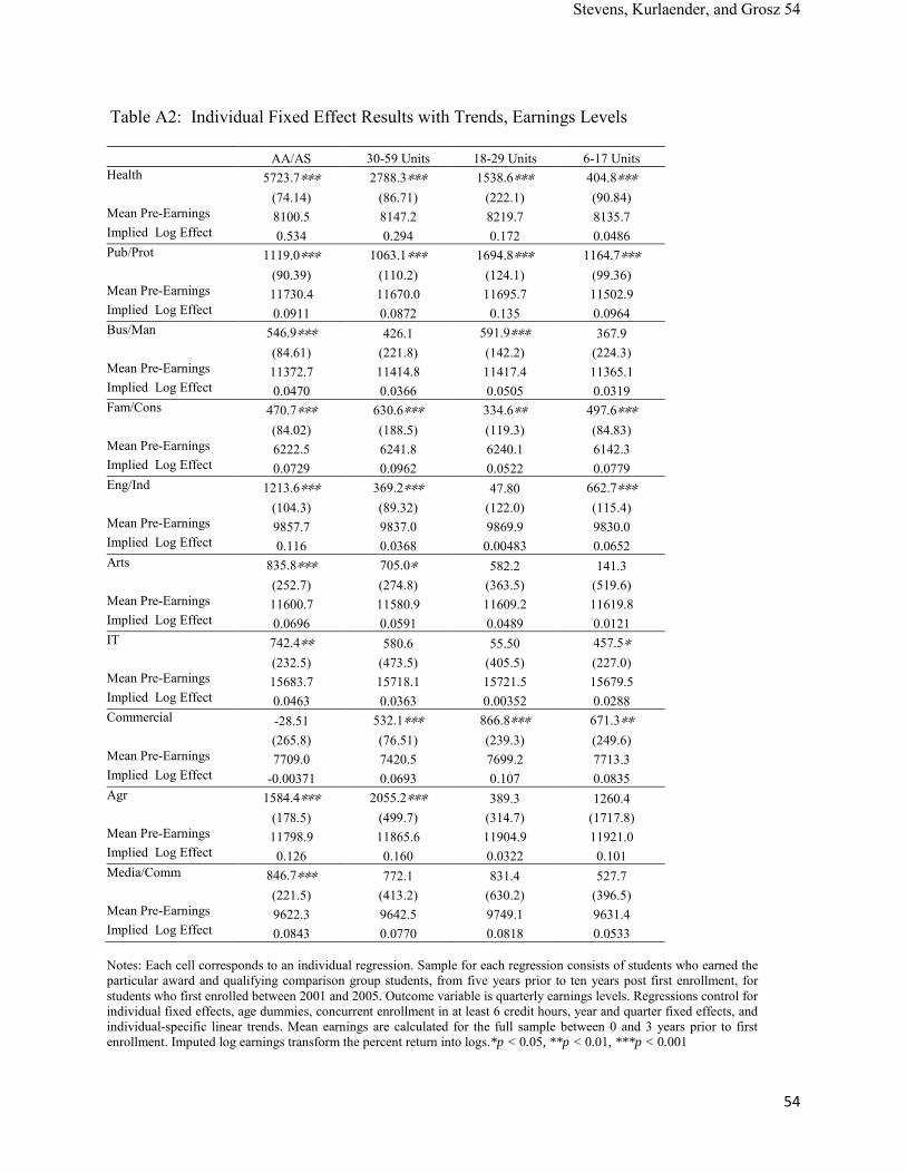
Stevens, Kurlaender, and Grosz 54
54
Table A2: Individual Fixed Effect Results with Trends, Earnings Levels AA/AS 30-59 Units 18-29 Units 6-17 Units Health 5723.7∗∗∗ 2788.3∗∗∗ 1538.6∗∗∗ 404.8∗∗∗ (74.14) (86.71) (222.1) (90.84) Mean Pre-Earnings 8100.5 8147.2 8219.7 8135.7 Implied Log Effect 0.534 0.294 0.172 0.0486 Pub/Prot 1119.0∗∗∗ 1063.1∗∗∗ 1694.8∗∗∗ 1164.7∗∗∗ (90.39) (110.2) (124.1) (99.36) Mean Pre-Earnings 11730.4 11670.0 11695.7 11502.9 Implied Log Effect 0.0911 0.0872 0.135 0.0964 Bus/Man 546.9∗∗∗ 426.1 591.9∗∗∗ 367.9 (84.61) (221.8) (142.2) (224.3) Mean Pre-Earnings 11372.7 11414.8 11417.4 11365.1 Implied Log Effect 0.0470 0.0366 0.0505 0.0319 Fam/Cons 470.7∗∗∗ 630.6∗∗∗ 334.6∗∗ 497.6∗∗∗ (84.02) (188.5) (119.3) (84.83) Mean Pre-Earnings 6222.5 6241.8 6240.1 6142.3 Implied Log Effect 0.0729 0.0962 0.0522 0.0779 Eng/Ind 1213.6∗∗∗ 369.2∗∗∗ 47.80 662.7∗∗∗ (104.3) (89.32) (122.0) (115.4) Mean Pre-Earnings 9857.7 9837.0 9869.9 9830.0 Implied Log Effect 0.116 0.0368 0.00483 0.0652 Arts 835.8∗∗∗ 705.0∗ 582.2 141.3 (252.7) (274.8) (363.5) (519.6) Mean Pre-Earnings 11600.7 11580.9 11609.2 11619.8 Implied Log Effect 0.0696 0.0591 0.0489 0.0121 IT 742.4∗∗ 580.6 55.50 457.5∗ (232.5) (473.5) (405.5) (227.0) Mean Pre-Earnings 15683.7 15718.1 15721.5 15679.5 Implied Log Effect 0.0463 0.0363 0.00352 0.0288 Commercial -28.51 532.1∗∗∗ 866.8∗∗∗ 671.3∗∗ (265.8) (76.51) (239.3) (249.6) Mean Pre-Earnings 7709.0 7420.5 7699.2 7713.3 Implied Log Effect -0.00371 0.0693 0.107 0.0835 Agr 1584.4∗∗∗ 2055.2∗∗∗ 389.3 1260.4 (178.5) (499.7) (314.7) (1717.8) Mean Pre-Earnings 11798.9 11865.6 11904.9 11921.0 Implied Log Effect 0.126 0.160 0.0322 0.101 Media/Comm 846.7∗∗∗ 772.1 831.4 527.7 (221.5) (413.2) (630.2) (396.5) Mean Pre-Earnings 9622.3 9642.5 9749.1 9631.4 Implied Log Effect 0.0843 0.0770 0.0818 0.0533 Notes: Each cell corresponds to an individual regression. Sample for each regression consists of students who earned the particular award and qualifying comparison group students, from five years prior to ten years post first enrollment, for students who first enrolled between 2001 and 2005. Outcome variable is quarterly earnings levels. Regressions control for individual fixed effects, age dummies, concurrent enrollment in at least 6 credit hours, year and quarter fixed effects, and individual-specific linear trends. Mean earnings are calculated for the full sample between 0 and 3 years prior to first enrollment. Imputed log earnings transform the percent return into logs.*p < 0.05, **p < 0.01, ***p < 0.001
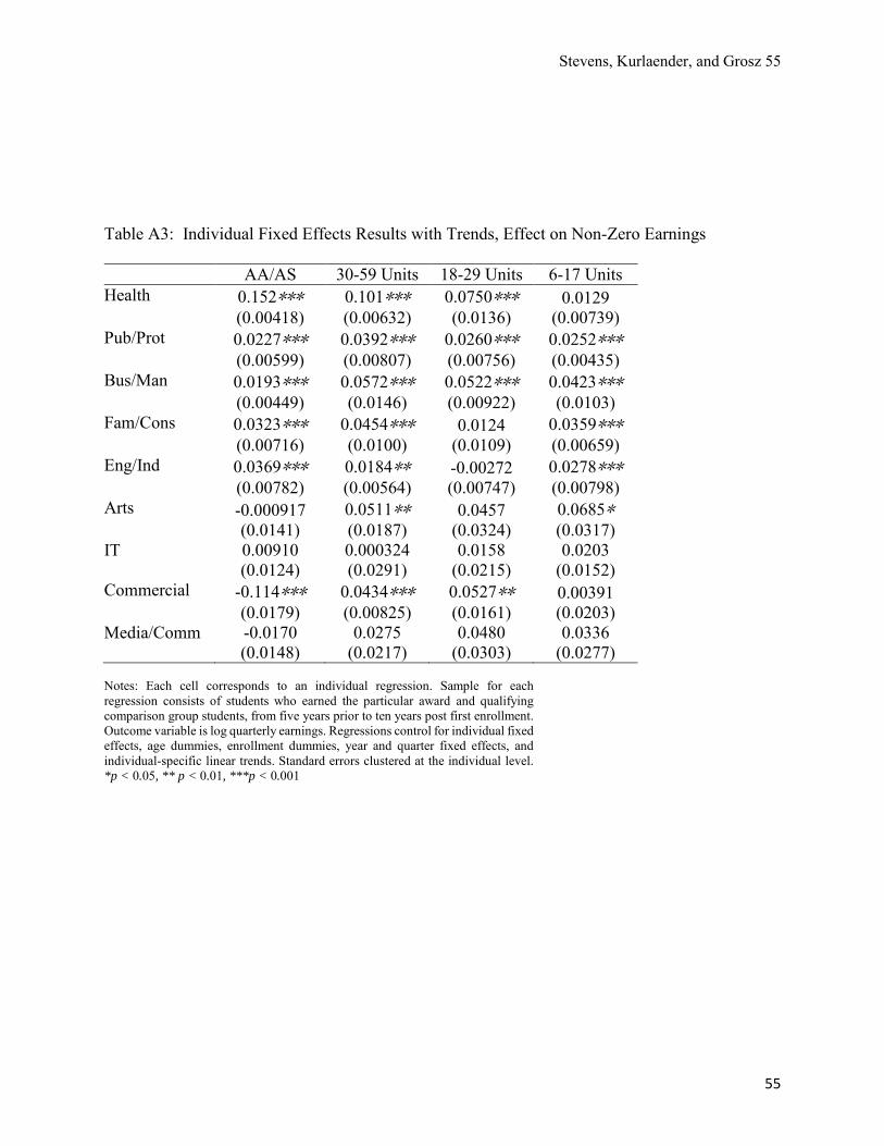
Stevens, Kurlaender, and Grosz 55
55
Table A3: Individual Fixed Effects Results with Trends, Effect on Non-Zero Earnings
AA/AS 30-59 Units 18-29 Units 6-17 Units Health 0.152∗∗∗ 0.101∗∗∗ 0.0750∗∗∗ 0.0129 Pub/Prot
(0.00418) 0.0227∗∗∗
(0.00632) 0.0392∗∗∗
(0.0136) 0.0260∗∗∗
(0.00739) 0.0252∗∗∗
Bus/Man
(0.00599) 0.0193∗∗∗
(0.00807) 0.0572∗∗∗
(0.00756) 0.0522∗∗∗
(0.00435) 0.0423∗∗∗
(0.00449) (0.0146) (0.00922) (0.0103) Fam/Cons 0.0323∗∗∗ 0.0454∗∗∗ 0.0124 0.0359∗∗∗ (0.00716) (0.0100) (0.0109) (0.00659) Eng/Ind 0.0369∗∗∗ 0.0184∗∗ -0.00272 0.0278∗∗∗ (0.00782) (0.00564) (0.00747) (0.00798) Arts -0.000917 0.0511∗∗ 0.0457 0.0685∗ (0.0141) (0.0187) (0.0324) (0.0317) IT 0.00910 0.000324 0.0158 0.0203 (0.0124) (0.0291) (0.0215) (0.0152) Commercial -0.114∗∗∗ 0.0434∗∗∗ 0.0527∗∗ 0.00391 (0.0179) (0.00825) (0.0161) (0.0203) Media/Comm -0.0170 0.0275 0.0480 0.0336 (0.0148) (0.0217) (0.0303) (0.0277) Notes: Each cell corresponds to an individual regression. Sample for each regression consists of students who earned the particular award and qualifying comparison group students, from five years prior to ten years post first enrollment. Outcome variable is log quarterly earnings. Regressions control for individual fixed effects, age dummies, enrollment dummies, year and quarter fixed effects, and individual-specific linear trends. Standard errors clustered at the individual level. *p < 0.05, ** p < 0.01, ***p < 0.001
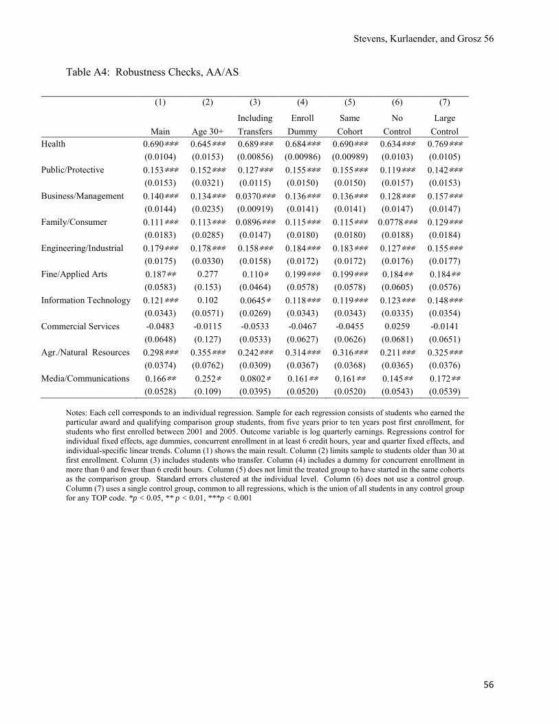
Stevens, Kurlaender, and Grosz 56
56
Table A4: Robustness Checks, AA/AS
Notes: Each cell corresponds to an individual regression. Sample for each regression consists of students who earned the particular award and qualifying comparison group students, from five years prior to ten years post first enrollment, for students who first enrolled between 2001 and 2005. Outcome variable is log quarterly earnings. Regressions control for individual fixed effects, age dummies, concurrent enrollment in at least 6 credit hours, year and quarter fixed effects, and individual-specific linear trends. Column (1) shows the main result. Column (2) limits sample to students older than 30 at first enrollment. Column (3) includes students who transfer. Column (4) includes a dummy for concurrent enrollment in more than 0 and fewer than 6 credit hours. Column (5) does not limit the treated group to have started in the same cohorts as the comparison group. Standard errors clustered at the individual level. Column (6) does not use a control group. Column (7) uses a single control group, common to all regressions, which is the union of all students in any control group for any TOP code. *p < 0.05, ** p < 0.01, ***p < 0.001
(1) (2) (3) (4) (5) (6) (7)
Including Enroll Same No Large Main Age 30+ Transfers Dummy Cohort Control Control
Health 0.690∗∗∗ 0.645∗∗∗ 0.689∗∗∗ 0.684∗∗∗ 0.690∗∗∗ 0.634∗∗∗ 0.769∗∗∗ (0.0104) (0.0153) (0.00856) (0.00986) (0.00989) (0.0103) (0.0105) Public/Protective 0.153∗∗∗ 0.152∗∗∗ 0.127∗∗∗ 0.155∗∗∗ 0.155∗∗∗ 0.119∗∗∗ 0.142∗∗∗ (0.0153) (0.0321) (0.0115) (0.0150) (0.0150) (0.0157) (0.0153) Business/Management 0.140∗∗∗ 0.134∗∗∗ 0.0370∗∗∗ 0.136∗∗∗ 0.136∗∗∗ 0.128∗∗∗ 0.157∗∗∗ (0.0144) (0.0235) (0.00919) (0.0141) (0.0141) (0.0147) (0.0147) Family/Consumer 0.111∗∗∗ 0.113∗∗∗ 0.0896∗∗∗ 0.115∗∗∗ 0.115∗∗∗ 0.0778∗∗∗ 0.129∗∗∗ (0.0183) (0.0285) (0.0147) (0.0180) (0.0180) (0.0188) (0.0184) Engineering/Industrial 0.179∗∗∗ 0.178∗∗∗ 0.158∗∗∗ 0.184∗∗∗ 0.183∗∗∗ 0.127∗∗∗ 0.155∗∗∗ (0.0175) (0.0330) (0.0158) (0.0172) (0.0172) (0.0176) (0.0177) Fine/Applied Arts 0.187∗∗ 0.277 0.110∗ 0.199∗∗∗ 0.199∗∗∗ 0.184∗∗ 0.184∗∗ (0.0583) (0.153) (0.0464) (0.0578) (0.0578) (0.0605) (0.0576) Information Technology 0.121∗∗∗ 0.102 0.0645∗ 0.118∗∗∗ 0.119∗∗∗ 0.123∗∗∗ 0.148∗∗∗ (0.0343) (0.0571) (0.0269) (0.0343) (0.0343) (0.0335) (0.0354) Commercial Services -0.0483 -0.0115 -0.0533 -0.0467 -0.0455 0.0259 -0.0141 (0.0648) (0.127) (0.0533) (0.0627) (0.0626) (0.0681) (0.0651) Agr./Natural Resources 0.298∗∗∗ 0.355∗∗∗ 0.242∗∗∗ 0.314∗∗∗ 0.316∗∗∗ 0.211∗∗∗ 0.325∗∗∗ (0.0374) (0.0762) (0.0309) (0.0367) (0.0368) (0.0365) (0.0376) Media/Communications 0.166∗∗ 0.252∗ 0.0802∗ 0.161∗∗ 0.161∗∗ 0.145∗∗ 0.172∗∗ (0.0528) (0.109) (0.0395) (0.0520) (0.0520) (0.0543) (0.0539)
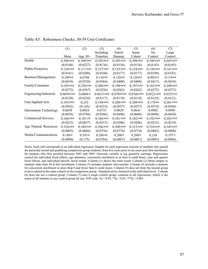
Stevens, Kurlaender, and Grosz 57
57
Table A5: Robustness Checks, 30-59 Unit Certificates (1) (2) (3) (4) (5) (6) (7) Including Enroll Same No Large Main Age 30+ Transfers Dummy Cohort Control Control Health 0.398∗∗∗ 0.399∗∗∗ 0.395∗∗∗ 0.395∗∗∗ 0.398∗∗∗ 0.396∗∗∗ 0.445∗∗∗ (0.0144) (0.0227) (0.0136) (0.0136) (0.0136) (0.0143) (0.0145) Public/Protective 0.154∗∗∗ 0.111∗∗∗ 0.157∗∗∗ 0.155∗∗∗ 0.154∗∗∗ 0.150∗∗∗ 0.141∗∗∗ (0.0181) (0.0280) (0.0160) (0.0177) (0.0177) (0.0190) (0.0181) Business/Management 0.109∗∗ 0.0788 0.110∗∗ 0.120∗∗ 0.120∗∗ 0.0925∗ 0.119∗∗ (0.0410) (0.0520) (0.0364) (0.0408) (0.0408) (0.0417) (0.0418) Family/Consumer 0.195∗∗∗ 0.228∗∗∗ 0.200∗∗∗ 0.198∗∗∗ 0.197∗∗∗ 0.162∗∗∗ 0.209∗∗∗ (0.0272) (0.0367) (0.0256) (0.0262) (0.0262) (0.0272) (0.0273) Engineering/Industrial 0.0659∗∗∗ 0.0484∗ 0.0615∗∗∗ 0.0789∗∗∗ 0.0760∗∗∗ 0.0522∗∗∗ 0.0335∗∗ (0.0120) (0.0220) (0.0117) (0.0118) (0.0118) (0.0125) (0.0121) Fine/Applied Arts 0.193∗∗∗ 0.253 0.194∗∗∗ 0.208∗∗∗ 0.209∗∗∗ 0.179∗∗ 0.201∗∗∗ (0.0562) (0.145) (0.0523) (0.0557) (0.0557) (0.0574) (0.0569) Information Technology 0.0659 0.0824 0.0733 0.0629 0.0641 0.0982 0.0994 (0.0638) (0.0794) (0.0586) (0.0608) (0.0608) (0.0698) (0.0650) Commercial Services 0.184∗∗∗ 0.181∗∗ 0.186∗∗∗ 0.181∗∗∗ 0.182∗∗∗ 0.192∗∗∗ 0.203∗∗∗ (0.0223) (0.0637) (0.0213) (0.0206) (0.0206) (0.0232) (0.0219) Agr./Natural Resources 0.324∗∗∗ 0.349∗∗∗ 0.296∗∗∗ 0.309∗∗∗ 0.312∗∗∗ 0.324∗∗∗ 0.345∗∗∗ (0.0803) (0.0866) (0.0756) (0.0774) (0.0774) (0.0882) (0.0800) Media/Communications 0.188∗ 0.393∗ 0.206∗∗ 0.200∗ 0.200∗ 0.158 0.197∗ (0.0890) (0.175) (0.0784) (0.0867) (0.0867) (0.0893) (0.0894) Notes: Each cell corresponds to an individual regression. Sample for each regression consists of students who earned the particular award and qualifying comparison group students, from five years prior to ten years post first enrollment, for students who first enrolled between 2001 and 2005. Outcome variable is log quarterly earnings. Regressions control for individual fixed effects, age dummies, concurrent enrollment in at least 6 credit hours, year and quarter fixed effects, and individual-specific linear trends. Column (1) shows the main result. Column (2) limits sample to students older than 30 at first enrollment. Column (3) includes students who transfer. Column (4) includes a dummy for concurrent enrollment in more than 0 and fewer than 6 credit hours. Column (5) does not limit the treated group to have started in the same cohorts as the comparison group. Standard errors clustered at the individual level. Column (6) does not use a control group. Column (7) uses a single control group, common to all regressions, which is the union of all students in any control group for any TOP code. *p < 0.05, **p < 0.01, ***p < 0.001
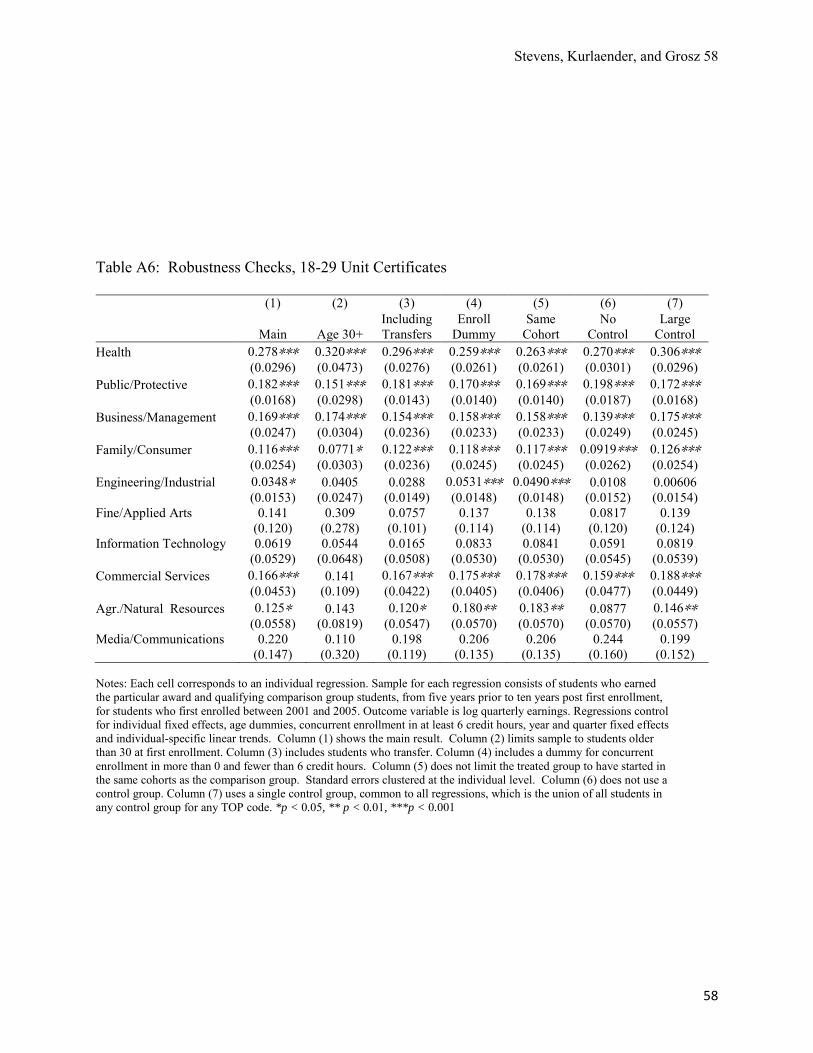
Stevens, Kurlaender, and Grosz 58
58
Table A6: Robustness Checks, 18-29 Unit Certificates (1) (2) (3) (4) (5) (6) (7) Including Enroll Same No Large Main Age 30+ Transfers Dummy Cohort Control Control Health 0.278∗∗∗ 0.320∗∗∗ 0.296∗∗∗ 0.259∗∗∗ 0.263∗∗∗ 0.270∗∗∗ 0.306∗∗∗ (0.0296) (0.0473) (0.0276) (0.0261) (0.0261) (0.0301) (0.0296) Public/Protective 0.182∗∗∗ 0.151∗∗∗ 0.181∗∗∗ 0.170∗∗∗ 0.169∗∗∗ 0.198∗∗∗ 0.172∗∗∗ (0.0168) (0.0298) (0.0143) (0.0140) (0.0140) (0.0187) (0.0168) Business/Management 0.169∗∗∗ 0.174∗∗∗ 0.154∗∗∗ 0.158∗∗∗ 0.158∗∗∗ 0.139∗∗∗ 0.175∗∗∗ (0.0247) (0.0304) (0.0236) (0.0233) (0.0233) (0.0249) (0.0245) Family/Consumer 0.116∗∗∗ 0.0771∗ 0.122∗∗∗ 0.118∗∗∗ 0.117∗∗∗ 0.0919∗∗∗ 0.126∗∗∗ (0.0254) (0.0303) (0.0236) (0.0245) (0.0245) (0.0262) (0.0254) Engineering/Industrial 0.0348∗ 0.0405 0.0288 0.0531∗∗∗ 0.0490∗∗∗ 0.0108 0.00606 (0.0153) (0.0247) (0.0149) (0.0148) (0.0148) (0.0152) (0.0154) Fine/Applied Arts 0.141 0.309 0.0757 0.137 0.138 0.0817 0.139 (0.120) (0.278) (0.101) (0.114) (0.114) (0.120) (0.124) Information Technology 0.0619 0.0544 0.0165 0.0833 0.0841 0.0591 0.0819 (0.0529) (0.0648) (0.0508) (0.0530) (0.0530) (0.0545) (0.0539) Commercial Services 0.166∗∗∗ 0.141 0.167∗∗∗ 0.175∗∗∗ 0.178∗∗∗ 0.159∗∗∗ 0.188∗∗∗ (0.0453) (0.109) (0.0422) (0.0405) (0.0406) (0.0477) (0.0449) Agr./Natural Resources 0.125∗ 0.143 0.120∗ 0.180∗∗ 0.183∗∗ 0.0877 0.146∗∗ (0.0558) (0.0819) (0.0547) (0.0570) (0.0570) (0.0570) (0.0557) Media/Communications 0.220 0.110 0.198 0.206 0.206 0.244 0.199 (0.147) (0.320) (0.119) (0.135) (0.135) (0.160) (0.152) Notes: Each cell corresponds to an individual regression. Sample for each regression consists of students who earned the particular award and qualifying comparison group students, from five years prior to ten years post first enrollment, for students who first enrolled between 2001 and 2005. Outcome variable is log quarterly earnings. Regressions control for individual fixed effects, age dummies, concurrent enrollment in at least 6 credit hours, year and quarter fixed effects and individual-specific linear trends. Column (1) shows the main result. Column (2) limits sample to students older than 30 at first enrollment. Column (3) includes students who transfer. Column (4) includes a dummy for concurrent enrollment in more than 0 and fewer than 6 credit hours. Column (5) does not limit the treated group to have started in the same cohorts as the comparison group. Standard errors clustered at the individual level. Column (6) does not use a control group. Column (7) uses a single control group, common to all regressions, which is the union of all students in any control group for any TOP code. *p < 0.05, ** p < 0.01, ***p < 0.001
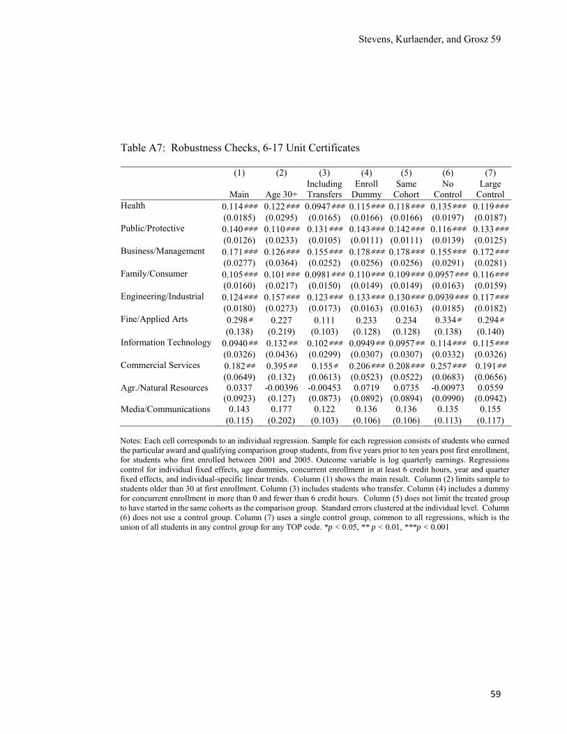
Stevens, Kurlaender, and Grosz 59
59
Table A7: Robustness Checks, 6-17 Unit Certificates (1) (2) (3) (4) (5) (6) (7) Including Enroll Same No Large Main Age 30+ Transfers Dummy Cohort Control Control Health 0.114∗∗∗ 0.122∗∗∗ 0.0947∗∗∗ 0.115∗∗∗ 0.118∗∗∗ 0.135∗∗∗ 0.119∗∗∗ (0.0185) (0.0295) (0.0165) (0.0166) (0.0166) (0.0197) (0.0187) Public/Protective 0.140∗∗∗ 0.110∗∗∗ 0.131∗∗∗ 0.143∗∗∗ 0.142∗∗∗ 0.116∗∗∗ 0.133∗∗∗ (0.0126) (0.0233) (0.0105) (0.0111) (0.0111) (0.0139) (0.0125) Business/Management 0.171∗∗∗ 0.126∗∗∗ 0.155∗∗∗ 0.178∗∗∗ 0.178∗∗∗ 0.155∗∗∗ 0.172∗∗∗ (0.0277) (0.0364) (0.0252) (0.0256) (0.0256) (0.0291) (0.0281) Family/Consumer 0.105∗∗∗ 0.101∗∗∗ 0.0981∗∗∗ 0.110∗∗∗ 0.109∗∗∗ 0.0957∗∗∗ 0.116∗∗∗ (0.0160) (0.0217) (0.0150) (0.0149) (0.0149) (0.0163) (0.0159) Engineering/Industrial 0.124∗∗∗ 0.157∗∗∗ 0.123∗∗∗ 0.133∗∗∗ 0.130∗∗∗ 0.0939∗∗∗ 0.117∗∗∗ (0.0180) (0.0273) (0.0173) (0.0163) (0.0163) (0.0185) (0.0182) Fine/Applied Arts 0.298∗ 0.227 0.111 0.233 0.234 0.334∗ 0.294∗ (0.138) (0.219) (0.103) (0.128) (0.128) (0.138) (0.140) Information Technology 0.0940∗∗ 0.132∗∗ 0.102∗∗∗ 0.0949∗∗ 0.0957∗∗ 0.114∗∗∗ 0.115∗∗∗ (0.0326) (0.0436) (0.0299) (0.0307) (0.0307) (0.0332) (0.0326) Commercial Services 0.182∗∗ 0.395∗∗ 0.155∗ 0.206∗∗∗ 0.208∗∗∗ 0.257∗∗∗ 0.191∗∗ (0.0649) (0.132) (0.0613) (0.0523) (0.0522) (0.0683) (0.0656) Agr./Natural Resources 0.0337 -0.00396 -0.00453 0.0719 0.0735 -0.00973 0.0559 (0.0923) (0.127) (0.0873) (0.0892) (0.0894) (0.0990) (0.0942) Media/Communications 0.143 0.177 0.122 0.136 0.136 0.135 0.155 (0.115) (0.202) (0.103) (0.106) (0.106) (0.113) (0.117) Notes: Each cell corresponds to an individual regression. Sample for each regression consists of students who earned the particular award and qualifying comparison group students, from five years prior to ten years post first enrollment, for students who first enrolled between 2001 and 2005. Outcome variable is log quarterly earnings. Regressions control for individual fixed effects, age dummies, concurrent enrollment in at least 6 credit hours, year and quarter fixed effects, and individual-specific linear trends. Column (1) shows the main result. Column (2) limits sample to students older than 30 at first enrollment. Column (3) includes students who transfer. Column (4) includes a dummy for concurrent enrollment in more than 0 and fewer than 6 credit hours. Column (5) does not limit the treated group to have started in the same cohorts as the comparison group. Standard errors clustered at the individual level. Column (6) does not use a control group. Column (7) uses a single control group, common to all regressions, which is the union of all students in any control group for any TOP code. *p < 0.05, ** p < 0.01, ***p < 0.001