This article was downloaded by: [North Dakota State University]On: 28 October 2014, At: 01:45Publisher: Taylor & FrancisInforma Ltd Registered in England and Wales Registered Number: 1072954 Registered office: Mortimer House,37-41 Mortimer Street, London W1T 3JH, UK

International Journal of Production ResearchPublication details, including instructions for authors and subscription information:http://www.tandfonline.com/loi/tprs20

CARI – a heuristic approach to machine-part cellformation using correlation analysis and relevanceindexN. Srinivasa Guptaa, Devika D.b, Valarmathi B.c, Sowmiya N.d & Apoorv Shindee

a Manufacturing Engineering Division, School of Mechanical Engineering and BuildingSciences, VIT University, Vellore, Indiab Department of Mechanical Engineering, Dr. N.G.P. Institute of Technology, Coimbatore,Indiac Soft Computing Division, School of Information Technology and Engineering, VIT University,Vellore, Indiad School of Information Technology and Engineering, VIT University, Vellore, Indiae School of Mechanical Engineering and Building Sciences, VIT University, Vellore, IndiaPublished online: 02 Jun 2014.

To cite this article: N. Srinivasa Gupta, Devika D., Valarmathi B., Sowmiya N. & Apoorv Shinde (2014): CARI – a heuristicapproach to machine-part cell formation using correlation analysis and relevance index, International Journal of ProductionResearch, DOI: 10.1080/00207543.2014.922709

To link to this article: http://dx.doi.org/10.1080/00207543.2014.922709

PLEASE SCROLL DOWN FOR ARTICLE

Taylor & Francis makes every effort to ensure the accuracy of all the information (the “Content”) containedin the publications on our platform. However, Taylor & Francis, our agents, and our licensors make norepresentations or warranties whatsoever as to the accuracy, completeness, or suitability for any purpose of theContent. Any opinions and views expressed in this publication are the opinions and views of the authors, andare not the views of or endorsed by Taylor & Francis. The accuracy of the Content should not be relied upon andshould be independently verified with primary sources of information. Taylor and Francis shall not be liable forany losses, actions, claims, proceedings, demands, costs, expenses, damages, and other liabilities whatsoeveror howsoever caused arising directly or indirectly in connection with, in relation to or arising out of the use ofthe Content.

This article may be used for research, teaching, and private study purposes. Any substantial or systematicreproduction, redistribution, reselling, loan, sub-licensing, systematic supply, or distribution in anyform to anyone is expressly forbidden. Terms & Conditions of access and use can be found at http://www.tandfonline.com/page/terms-and-conditions

CARI – a heuristic approach to machine-part cell formation using correlation analysis andrelevance index

N. Srinivasa Guptaa*, Devika D.b, Valarmathi B.c, Sowmiya N.d and Apoorv Shindee

aManufacturing Engineering Division, School of Mechanical Engineering and Building Sciences, VIT University, Vellore, India;bDepartment of Mechanical Engineering, Dr. N.G.P. Institute of Technology, Coimbatore, India; cSoft Computing Division, School ofInformation Technology and Engineering, VIT University, Vellore, India; dSchool of Information Technology and Engineering, VIT

University, Vellore, India; eSchool of Mechanical Engineering and Building Sciences, VIT University, Vellore, India

(Received 27 May 2013; accepted 2 May 2014)

Machine-part cell formation is the process of identifying part families and the appropriate machine cell for each partfamily. Grouping efficacy (GE), the widely used measure for assessing the goodness of the machine-part cells dependson identification of correct part families and the appropriate machine cell for each part family. In this paper, a heuristicbased on correlation analysis and relevance index is proposed for the formation of machine-part cells. Computationalperformance of the proposed heuristic on a set of group technology data-set available in the literature is also presented.GE of the solutions produced by the proposed heuristic is equal to the best efficacy reported in the literature for 63% ofthe test instances and improved the GE for 6% of the total test instances.

Keywords: machine-part cell formation; cellular manufacturing; correlation analysis; relevance index; grouping efficacy

1. Introduction

Cellular manufacturing has been the topic of research for more than three decades and it continues to be an attractivefield of research. The production volume advantage of product layout and product variety advantage of process layoutare effectively combined in the cellular layout as the parts that have similar machining requirements are grouped as partfamilies and they are manufactured in exclusive cells consisting of only the appropriate machines. This results in a mini-mal material-handling cost and enhanced productivity. The firms that have adopted cellular manufacturing system(CMS) have reported a reduction in the material-handling cost, production lead time and enhanced productivity (Hyerand Wemmerlov 1989). The companies that have stable demand for their product, high material-handling cost and highratio of operation time to set-up time can be benefited by changing from batch production to cellular manufacturing(Burges, Morgan, and Vollmann 1993). In the context of CMS design, grouping of parts into part families and machinesinto machine cells is very crucial and is known as machine-part cell formation (MPCF). Ballakur and Steudel (1987)demonstrated that finding the best part families and the appropriate machine cells is certainly an NP-complete problem.

The strategies for MPCF addressed in the literature can be broadly classified as follows:

(1) part family grouping solution strategies, in which the part families are formed first and followed by themachine-cell creation for the part families,

(2) machine grouping solution strategies, in which machine cells are created first and parts are allocated after that,and

(3) simultaneous machine-part grouping solution strategies.

Part family grouping solution strategies cannot be used a stand-alone procedure for finding part families becausethey group parts that are similar in shape but differ in size or tolerances and hence the parts in a family may getmachined in different cells. Machine grouping solution strategies are carried out in two phases. In the first phase,machines are grouped based on the inference from the part routing. In the second phase, parts are allocated to cells andthe cells are re-evaluated based on additional factors such as machine utilisation. Simultaneous machine-part groupingsolution strategies involve the concurrent formation of part families and machine cells. The various methods found inthe literature on MPCF can be classified into manual methods, algorithmic methods and combinatorial methods.

*Corresponding author. Email: srinivasagupta.n@vit.ac.in

© 2014 Taylor & Francis

International Journal of Production Research, 2014http://dx.doi.org/10.1080/00207543.2014.922709

Dow

nloa

ded

by [

Nor

th D

akot

a St

ate

Uni

vers

ity]

at 0

1:45

28

Oct

ober

201

4

Subjective evaluation of the layout designer is required while using the manual methods like production flow analysis(PFA). Algorithmic methods like ZODIAC (Chandrasekharan and Rajagopalan 1987) and GRAFICS (Srinivasan andNarendran 1991) followed the machine-part grouping solution strategy. The other methods like minimum spanningtrees-based clustering algorithm (referred to as MST) proposed by Srinivasan (1994), travelling salesman problem-basedgenetic algorithm (referred to as GA-TSP) proposed by Cheng et al. (1998), genetic programming (referred to as GP)proposed by Dimopoulos and Mort (2001), genetic algorithm (referred to as GA1) proposed by Onwubolu and Mutingi(2001), genetic algorithm (referred to as GA2) proposed by Gonçalves and Resende (2004) and ant colony algorithmproposed by Megala, Rajendran, and Gopalan (2008) followed the machine grouping strategy.

Burbidge (1971) introduced the concept of PFA for cell formation, which involved lot of manual calculations. PFAmethod required a rerun with the whole set of data if a new part is introduced. Hence, large-sized problems could notbe solved using this technique. King (1980) proposed an array-based method popularly known as rank order clustering(ROC), which used the machine-part incidence matrix (MPIM) as input for forming the machine-part cells. A modifiedversion of ROC was proposed by King and Nakornchai (1982), which is known as ROC2 algorithm. It should be notedthat the solution achieved by array-based methods is strongly influenced by the initial structure of the MPIM.

MPCF based on clustering analysis was introduced by McAuley (1972), who developed an algorithm based on sin-gle-linkage clustering and Seifoddini (1989) developed the average linkage clustering algorithm. Chandrasekharan andRajagopalan (1986a), Srinivasan, Narendran, and Mahadevan (1990), Nair and Narendran (1998), and George,Rajendran, and Ghosh (2003) proposed MPCF algorithms based on non-hierarchical clustering. Srinivasan, Narendran,and Mahadevan (1990) developed an assignment model for the cell formation problem. Adil, Rajamani, and Strong(1996) developed a non-linear integer programming model for the cell-formation problem. Hachicha, Masmoudi, andHaddar (2008) used correlation matrix and principal component analysis for forming the cells. Exceptional parts andexceptional machines were assigned using the angle measure and Euclidean distance (ED).

Gupta and Devika (2011) suggested a new method for the MPCF using Mahalanobis distance (MD). After identify-ing the part families and rearranging the MPIM as per the part families, the machines are arranged in the ascendingorder of their MD values and the final solution is achieved by resolving the bottleneck machines. MD is a superior sta-tistical measure when compared to the ED used for clustering analysis. Since, MD is based on the correlation amongthe various dimensions of the given problem; it gives the true representation of similarity among the dimensions underconsideration (Taguchi and Jugulum 2002).

To the best of our knowledge, the combination of correlation analysis (CA) for part family formation and relevanceindex (RI), a measure based on the number of exceptional elements and the number of voids that would be created dueto the allocation of a machine for a part family, has not been reported in the literature. For the first time, the proposedmethod based on correlation analysis and relevance index (CARI) is used for MPCF. Computational performance of theproposed CARI heuristic is assessed by solving 35 benchmark data-set problems gathered from the literature. GEachieved by CARI is promising and it improved the grouping efficacy (GE) for 6% of the total test instances.

2. Problem definition and measure of performance

In this paper, an attempt has been made to solve the MPCF problem as a zero-one block diagonalisation problem withan objective to minimise the intercellular movement of parts and to maximise the utilisation of machines within a cell.

Quality of the machine-part grouping is assessed by GE, proposed by Kumar and Chandrasekaran (1990). The for-mula for calculating GE is given in Equation (1).

GE ¼ ðN1 � N out1 Þ=ðN1 þ N in

0 Þ (1)

where N1 = total number of 1s in the matrix; Nout1 = total number of 1s outside the diagonal blocks (Exceptional ele-

ments); N in0 = total number of 0s inside the diagonal blocks (Voids).

Grouping efficiency proposed by Chandrasekharan and Rajagopalan (1989) is another popular grouping measureavailable in the literature. Due to its poor discriminating capability i.e. the ability to distinguish good quality groupingfrom the bad, it is not used in this paper.

3. CARI heuristic – the new approach

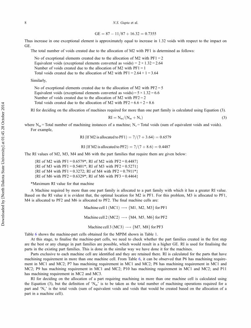
CARI, the heuristic proposed in this paper combines CA and RI for the MPCF. Figure 1 shows the sequence of stepsinvolved in the CARI heuristic in the form of a flow chart.

The major steps involved in the proposed algorithm are as follows:

2 N.S. Gupta et al.

Dow

nloa

ded

by [

Nor

th D

akot

a St

ate

Uni

vers

ity]

at 0

1:45

28

Oct

ober

201

4

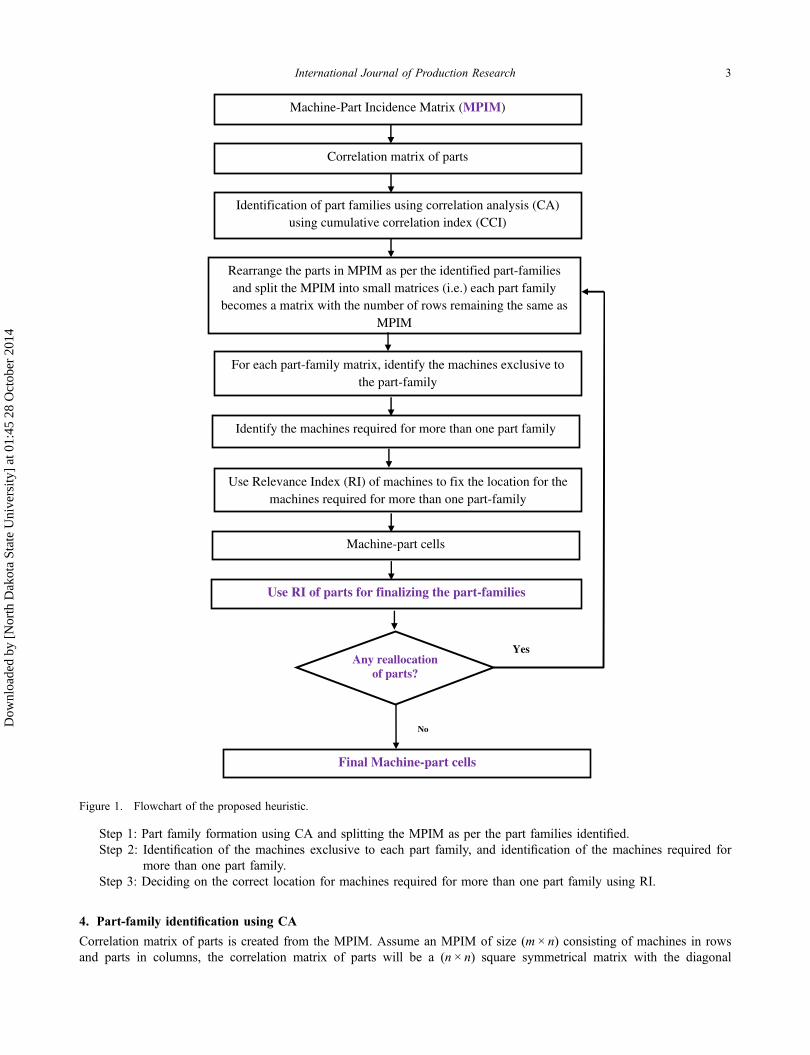
Step 1: Part family formation using CA and splitting the MPIM as per the part families identified.Step 2: Identification of the machines exclusive to each part family, and identification of the machines required for

more than one part family.Step 3: Deciding on the correct location for machines required for more than one part family using RI.

4. Part-family identification using CA

Correlation matrix of parts is created from the MPIM. Assume an MPIM of size (m × n) consisting of machines in rowsand parts in columns, the correlation matrix of parts will be a (n × n) square symmetrical matrix with the diagonal

Machine-Part Incidence Matrix (MPIM)

Correlation matrix of parts

Identification of part families using correlation analysis (CA) using cumulative correlation index (CCI)

Rearrange the parts in MPIM as per the identified part-families and split the MPIM into small matrices (i.e.) each part family

becomes a matrix with the number of rows remaining the same as MPIM

For each part-family matrix, identify the machines exclusive to the part-family

Identify the machines required for more than one part family

Use Relevance Index (RI) of machines to fix the location for the machines required for more than one part-family

Machine-part cells

Use RI of parts for finalizing the part-families

Final Machine-part cells

Any reallocation of parts?

Yes

No

Figure 1. Flowchart of the proposed heuristic.

International Journal of Production Research 3

Dow

nloa

ded

by [

Nor

th D

akot

a St

ate

Uni

vers

ity]

at 0

1:45

28

Oct

ober

201

4

elements equal to 1. The ijth element in the correlation matrix represents the correlation coefficient between the ith andjth vector. The diagonal elements (correlations of variables with themselves) are always equal to 1. In this paper, theMPIM is expressed with machines in rows and parts in columns. The correlation matrix of the MPIM is calculatedusing the ‘corrcoef’ function available as a built-in function in the MATLAB software.

The correlation coefficient is used as the measure of similarity. The correlation value varies from –1 to +1. ‘0’ corre-lation between two parts indicates that there is no relationship, ‘+1’ correlation indicates the perfect linear relationshipand ‘–1’ correlation indicates perfect linear negative relationship between the two parts. Parts that are positively corre-lated are grouped to form the part families. The procedure for the identification of the part families is explained in thesubsequent paragraphs.

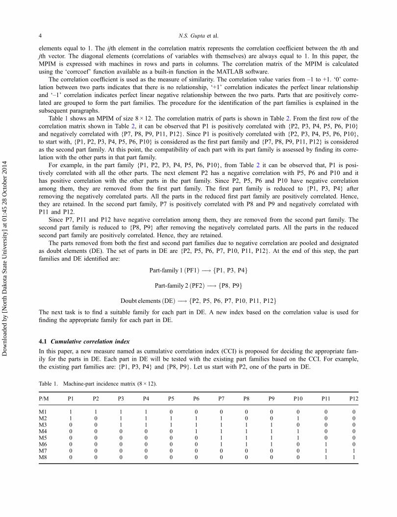
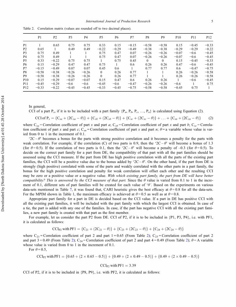
Table 1 shows an MPIM of size 8 × 12. The correlation matrix of parts is shown in Table 2. From the first row of thecorrelation matrix shown in Table 2, it can be observed that P1 is positively correlated with {P2, P3, P4, P5, P6, P10}and negatively correlated with {P7, P8, P9, P11, P12}. Since P1 is positively correlated with {P2, P3, P4, P5, P6, P10},to start with, {P1, P2, P3, P4, P5, P6, P10} is considered as the first part family and {P7, P8, P9, P11, P12} is consideredas the second part family. At this point, the compatibility of each part with its part family is assessed by finding its corre-lation with the other parts in that part family.

For example, in the part family {P1, P2, P3, P4, P5, P6, P10}, from Table 2 it can be observed that, P1 is posi-tively correlated with all the other parts. The next element P2 has a negative correlation with P5, P6 and P10 and ithas positive correlation with the other parts in the part family. Since P2, P5, P6 and P10 have negative correlationamong them, they are removed from the first part family. The first part family is reduced to {P1, P3, P4} afterremoving the negatively correlated parts. All the parts in the reduced first part family are positively correlated. Hence,they are retained. In the second part family, P7 is positively correlated with P8 and P9 and negatively correlated withP11 and P12.

Since P7, P11 and P12 have negative correlation among them, they are removed from the second part family. Thesecond part family is reduced to {P8, P9} after removing the negatively correlated parts. All the parts in the reducedsecond part family are positively correlated. Hence, they are retained.

The parts removed from both the first and second part families due to negative correlation are pooled and designatedas doubt elements (DE). The set of parts in DE are {P2, P5, P6, P7, P10, P11, P12}. At the end of this step, the partfamilies and DE identified are:

Part-family 1 ðPF1Þ �! fP1; P3; P4g

Part-family 2 ðPF2Þ �! fP8; P9g

Doubt elements ðDEÞ �! fP2; P5; P6; P7; P10; P11; P12gThe next task is to find a suitable family for each part in DE. A new index based on the correlation value is used forfinding the appropriate family for each part in DE.

4.1 Cumulative correlation index

In this paper, a new measure named as cumulative correlation index (CCI) is proposed for deciding the appropriate fam-ily for the parts in DE. Each part in DE will be tested with the existing part families based on the CCI. For example,the existing part families are: {P1, P3, P4} and {P8, P9}. Let us start with P2, one of the parts in DE.

Table 1. Machine-part incidence matrix (8 × 12).

P/M P1 P2 P3 P4 P5 P6 P7 P8 P9 P10 P11 P12

M1 1 1 1 1 0 0 0 0 0 0 0 0M2 1 0 1 1 1 1 1 0 0 1 0 0M3 0 0 1 1 1 1 1 1 1 0 0 0M4 0 0 0 0 0 1 1 1 1 1 0 0M5 0 0 0 0 0 0 1 1 1 1 0 0M6 0 0 0 0 0 0 1 1 1 0 1 0M7 0 0 0 0 0 0 0 0 0 0 1 1M8 0 0 0 0 0 0 0 0 0 0 1 1

4 N.S. Gupta et al.

Dow

nloa

ded

by [

Nor

th D

akot

a St

ate

Uni

vers

ity]

at 0

1:45

28

Oct

ober

201

4

In general,CCI of a part Px, if it is to be included with a part family {Pa, Pb, Pc, …, Pn} is calculated using Equation (2).

CCI of Px ¼ fCxa þ ð2Cxa � hÞg þ fCxb þ ð2Cxb � hÞg þ fCxc þ ð2Cxc � hÞg þ . . .þ fCxn þ ð2Cxn � hÞg (2)

where Cxa = Correlation coefficient of part x and part a; Cxb = Correlation coefficient of part x and part b; Cxc = Correla-tion coefficient of part x and part c; Cxn = Correlation coefficient of part x and part n; θ = a variable whose value is var-ied from 0 to 1 in the increment of 0.1.

‘2C – θ’ becomes a bonus for the parts with strong positive correlation and it becomes a penalty for the parts withweak correlation. For example, if the correlation (C) of two parts is 0.9, then the ‘2C – θ’ will become a bonus of 1.3(for θ = 0.5). If the correlation of two parts is 0.1, then the ‘2C – θ’ will become a penalty of –0.3 (for θ = 0.5). Todecide on the correct part family for a part from DE, the compatibility of that part with all the part families should beassessed using the CCI measure. If the part from DE has high positive correlation with all the parts of the existing partfamilies, the CCI will be a positive value due to the bonus added by ‘2C – θ’. On the other hand, if the part from DE isstrongly (high positive) correlated with some of the parts and weakly correlated with the other parts in a part family, thebonus for the high positive correlation and penalty for weak correlation will offset each other and the resulting CCImay be zero or a positive value or a negative value. With which existing part family, the part from DE will have bettercompatibility? This is answered by the CCI measure of that part. Since the θ value is varied from 0.1 to 1 in the incre-ment of 0.1, different sets of part families will be created for each value of ‘θ’. Based on the experiments on variousdata-sets mentioned in Table 7, it was found that, CARI heuristic gives the best efficacy at θ = 0.8 for all the data-sets.For the MPIM shown in Table 1, the maximum efficacy is achieved at θ = 0.5 as well as at θ = 0.8.

Appropriate part family for a part in DE is decided based on the CCI value. If a part in DE has positive CCI withall the existing part families, it will be included with the part family with which the largest CCI is obtained. In case ofa tie, the part is added with any one of the families. In case, if the part has negative CCI with all the existing part fami-lies, a new part family is created with that part as the first member.

For example, let us consider the part P2 from DE. CCI of P2, if it is to be included in {P1, P3, P4}, i.e. with PF1,it is calculated as follows:

CCIP2 with PF1 ¼ fC21 þ ð2C21 � hÞg þ fC23 þ ð2C23 � hÞg þ fC24 þ ð2C24 � hÞgwhere C21 = Correlation coefficient of part 2 and part 1 = 0.65 (From Table 2); C23 = Correlation coefficient of part 2and part 3 = 0.49 (From Table 2); C24 = Correlation coefficient of part 2 and part 4 = 0.49 (From Table 2); θ = A variablewhose value is varied from 0 to 1 in the increment of 0.1.

For θ = 0.5,

CCIP2 with PF1 ¼ f0:65þ ð2� 0:65� 0:5Þg þ f0:49þ ð2� 0:49� 0:5Þg þ f0:49þ ð2� 0:49� 0:5Þg

CCIP2 with PF1 ¼ 3:39

CCI of P2, if it is to be included in {P8, P9}, i.e. with PF2, it is calculated as follows:

Table 2. Correlation matrix (values are rounded off to two decimal places).

P1 P2 P3 P4 P5 P6 P7 P8 P9 P10 P11 P12

P1 1 0.65 0.75 0.75 0.33 0.15 −0.15 −0.58 −0.58 0.15 −0.45 −0.33P2 0.65 1 0.49 0.49 −0.22 −0.29 −0.49 −0.38 −0.38 −0.29 −0.29 −0.22P3 0.75 0.49 1 1 0.75 0.47 0.07 −0.26 −0.26 −0.07 −0.6 −0.45P4 0.75 0.49 1 1 0.75 0.47 0.07 −0.26 −0.26 −0.07 −0.6 −0.45P5 0.33 −0.22 0.75 0.75 1 0.75 0.45 0 0 0.15 −0.45 −0.33P6 0.15 −0.29 0.47 0.47 0.75 1 0.6 0.26 0.26 0.47 −0.6 −0.45P7 −0.15 −0.49 0.07 0.07 0.45 0.6 1 0.77 0.77 0.6 −0.47 −0.75P8 −0.58 −0.38 −0.26 −0.26 0 0.26 0.77 1 1 0.26 −0.26 −0.58P9 −0.58 −0.38 −0.26 −0.26 0 0.26 0.77 1 1 0.26 −0.26 −0.58P10 0.15 −0.29 −0.07 −0.07 0.15 0.47 0.6 0.26 0.26 1 −0.6 −0.45P11 −0.45 −0.29 −0.6 −0.6 −0.45 −0.6 −0.47 −0.26 −0.26 −0.6 1 0.75P12 −0.33 −0.22 −0.45 −0.45 −0.33 −0.45 −0.75 −0.58 −0.58 −0.45 0.75 1

International Journal of Production Research 5

Dow

nloa

ded

by [

Nor

th D

akot

a St

ate

Uni

vers

ity]

at 0

1:45

28

Oct

ober

201

4

CCIP2 with PF2 ¼ fC28 þ ð2C28 � hÞg þ fC29 þ ð2C29 � hÞg

CCIP2 with PF2 ¼ f�0:38þ ð2� ð�0:38Þ � 0:5Þg þ f�0:38þ ð2� ð�0:38Þ � 0:5Þg

CCIP2 with PF2 ¼ �3:28

Since CCIP2 with PF1 is higher than CCIP2 with PF2, the correct part family for P2 is PF1.After including P2 with PF1 the updated part families and DE are shown below:

Part-family 1 ðPF1Þ �! fP1; P3; P4; P2g

Part-family 2 ðPF2Þ �! fP8; P9g

Doubt elements ðDEÞ �! fP5; P6; P7; P10; P11; P12gThe next part in DE is P5, the correct part family for part P5 in DE can be decided by calculating CCI of P5 with theupdated PF1 and PF2. This procedure is repeated until the correct part families are found for all the parts in DE. Thefinal part families are:

PF1 �! fP1 P3 P4 P2 P5 P6g

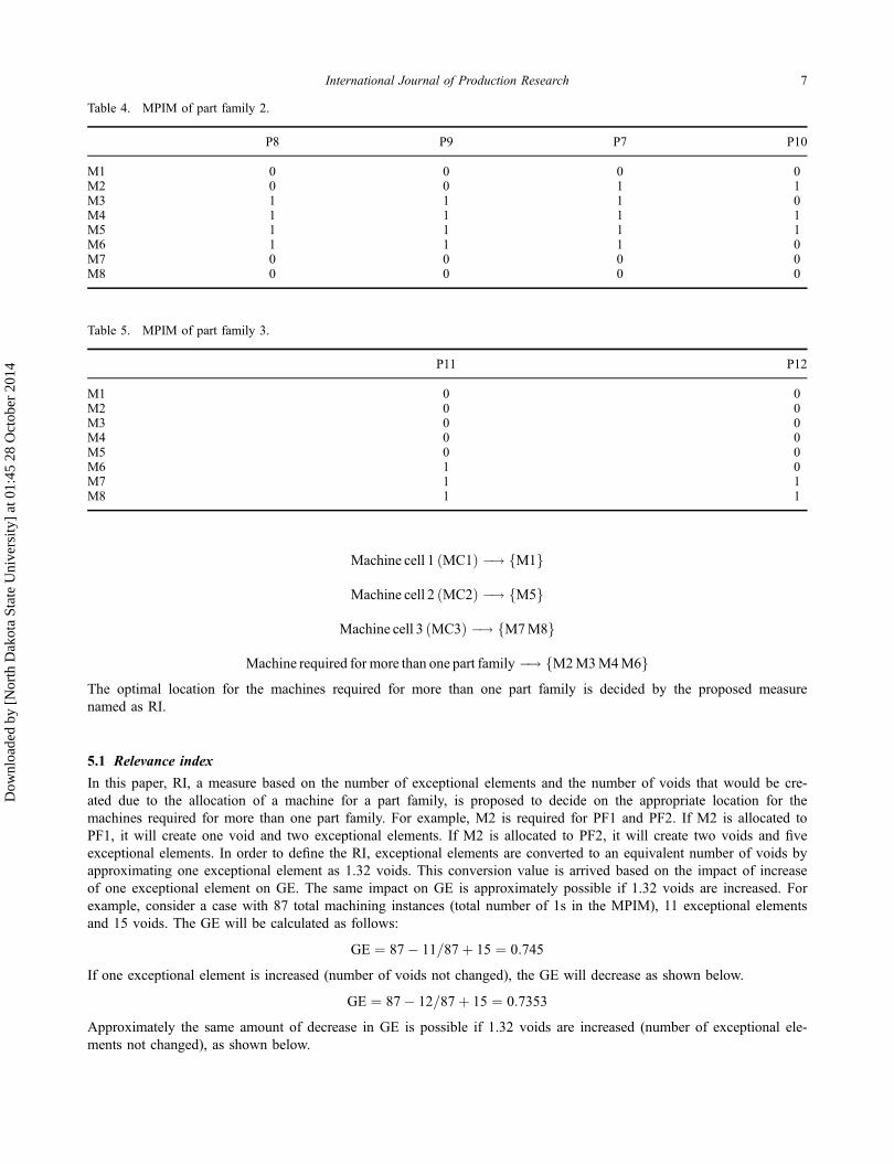
PF2 �! fP8 P9 P7 P10g

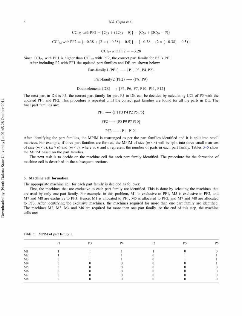
PF3 �! fP11 P12gAfter identifying the part families, the MPIM is rearranged as per the part families identified and it is split into smallmatrices. For example, if three part families are formed, the MPIM of size (m × n) will be split into three small matricesof size (m × a), (m × b) and (m × c), where a, b and c represent the number of parts in each part family. Tables 3–5 showthe MPIM based on the part families.

The next task is to decide on the machine cell for each part family identified. The procedure for the formation ofmachine cell is described in the subsequent sections.

5. Machine cell formation

The appropriate machine cell for each part family is decided as follows:First, the machines that are exclusive to each part family are identified. This is done by selecting the machines that

are used by only one part family. For example, in this problem, M1 is exclusive to PF1, M5 is exclusive to PF2, andM7 and M8 are exclusive to PF3. Hence, M1 is allocated to PF1, M5 is allocated to PF2, and M7 and M8 are allocatedto PF3. After identifying the exclusive machines, the machines required for more than one part family are identified.The machines M2, M3, M4 and M6 are required for more than one part family. At the end of this step, the machinecells are:

Table 3. MPIM of part family 1.

P1 P3 P4 P2 P5 P6

M1 1 1 1 1 0 0M2 1 1 1 0 1 1M3 0 1 1 0 1 1M4 0 0 0 0 0 1M5 0 0 0 0 0 0M6 0 0 0 0 0 0M7 0 0 0 0 0 0M8 0 0 0 0 0 0

6 N.S. Gupta et al.

Dow

nloa

ded

by [

Nor

th D

akot

a St

ate

Uni

vers

ity]

at 0

1:45

28

Oct

ober

201

4

Machine cell 1 ðMC1Þ �! fM1g

Machine cell 2 ðMC2Þ �! fM5g

Machine cell 3 ðMC3Þ �! fM7M8g

Machine required for more than one part family �! fM2M3M4M6gThe optimal location for the machines required for more than one part family is decided by the proposed measurenamed as RI.

5.1 Relevance index

In this paper, RI, a measure based on the number of exceptional elements and the number of voids that would be cre-ated due to the allocation of a machine for a part family, is proposed to decide on the appropriate location for themachines required for more than one part family. For example, M2 is required for PF1 and PF2. If M2 is allocated toPF1, it will create one void and two exceptional elements. If M2 is allocated to PF2, it will create two voids and fiveexceptional elements. In order to define the RI, exceptional elements are converted to an equivalent number of voids byapproximating one exceptional element as 1.32 voids. This conversion value is arrived based on the impact of increaseof one exceptional element on GE. The same impact on GE is approximately possible if 1.32 voids are increased. Forexample, consider a case with 87 total machining instances (total number of 1s in the MPIM), 11 exceptional elementsand 15 voids. The GE will be calculated as follows:

GE ¼ 87� 11=87þ 15 ¼ 0:745

If one exceptional element is increased (number of voids not changed), the GE will decrease as shown below.

GE ¼ 87� 12=87þ 15 ¼ 0:7353

Approximately the same amount of decrease in GE is possible if 1.32 voids are increased (number of exceptional ele-ments not changed), as shown below.

Table 4. MPIM of part family 2.

P8 P9 P7 P10

M1 0 0 0 0M2 0 0 1 1M3 1 1 1 0M4 1 1 1 1M5 1 1 1 1M6 1 1 1 0M7 0 0 0 0M8 0 0 0 0

Table 5. MPIM of part family 3.

P11 P12

M1 0 0M2 0 0M3 0 0M4 0 0M5 0 0M6 1 0M7 1 1M8 1 1

International Journal of Production Research 7

Dow

nloa

ded

by [

Nor

th D

akot

a St

ate

Uni

vers

ity]

at 0

1:45

28

Oct

ober

201

4

GE ¼ 87� 11=87þ 16:32 ¼ 0:7355

Thus increase in one exceptional element is approximately equal to increase in 1.32 voids with respect to the impact onGE.

The total number of voids created due to the allocation of M2 with PF1 is determined as follows:

No of exceptional elements created due to the allocation of M2 with PF1 = 2Equivalent voids (exceptional elements converted as voids) = 2 × 1.32 = 2.64Number of voids created due to the allocation of M2 with PF1 = 1Total voids created due to the allocation of M2 with PF1 = 2.64 + 1 = 3.64

Similarly,

No of exceptional elements created due to the allocation of M2 with PF2 = 5Equivalent voids (exceptional elements converted as voids) = 5 × 1.32 = 6.6Number of voids created due to the allocation of M2 with PF2 = 2Total voids created due to the allocation of M2 with PF2 = 6.6 + 2 = 8.6

RI for deciding on the allocation of machines required for more than one part family is calculated using Equation (3).

RI ¼ Nm=ðNm þ NvÞ (3)

where Nm = Total number of machining instances of a machine; Nv = Total voids (sum of equivalent voids and voids).For example,

RI ðIf M2 is allocated to PF1Þ ¼ 7=ð7þ 3:64Þ ¼ 0:6579

RI ðIf M2 is allocated to PF2Þ ¼ 7=ð7þ 8:6Þ ¼ 0:4487

The RI values of M2, M3, M4 and M6 with the part families that require them are given below:

{RI of M2 with PF1 = 0.6579*; RI of M2 with PF2 = 0.4487}{RI of M3 with PF1 = 0.5401*; RI of M3 with PF2 = 0.5271}{RI of M4 with PF1 = 0.3272; RI of M4 with PF2 = 0.7911*}{RI of M6 with PF2 = 0.6329*; RI of M6 with PF3 = 0.4464}

*Maximum RI value for that machine

A Machine required by more than one part family is allocated to a part family with which it has a greater RI value.Based on the RI value it is evident that, the optimal location for M2 is PF1. For this problem, M3 is allocated to PF1,M4 is allocated to PF2 and M6 is allocated to PF2. The final machine cells are:

Machine cell 1 ðMC1Þ �! fM1; M2; M3g for PF1

Machine cell 2 ðMC2Þ �! fM4; M5; M6g for PF2

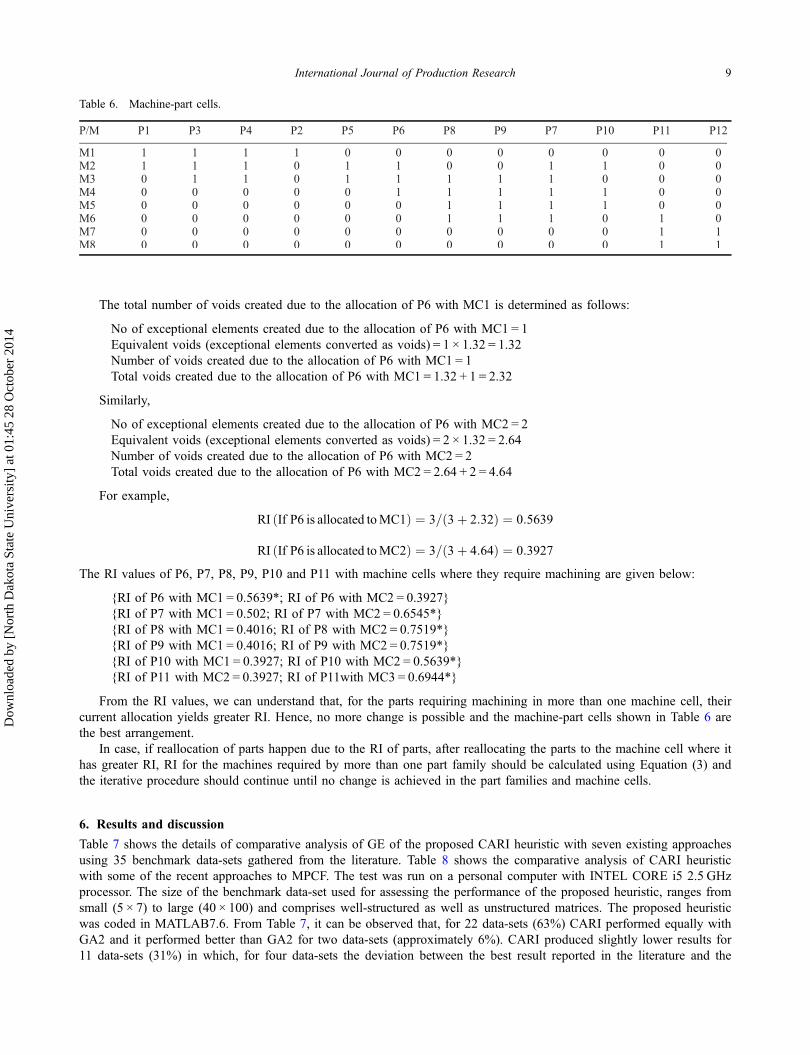
Machine cell 3 ðMC3Þ �! fM7; M8g for PF3Table 6 shows the machine-part cells obtained for the MPIM shown in Table 1.

At this stage, to finalise the machine-part cells, we need to check whether the part families created in the first stepare the best or any change in part families are possible, which would result in a higher GE. RI is used for finalising theparts in the existing part families. This is done in the similar way we have done it for the machines.

Parts exclusive to each machine cell are identified and they are retained there. RI is calculated for the parts that havemachining requirement in more than one machine cell. From Table 6, it can be observed that P6 has machining require-ment in MC1 and MC2; P7 has machining requirement in MC1 and MC2; P8 has machining requirement in MC1 andMC2; P9 has machining requirement in MC1 and MC2; P10 has machining requirement in MC1 and MC2; and P11has machining requirement in MC2 and MC3.

RI for deciding on the allocation of a part requiring machining in more than one machine cell is calculated usingthe Equation (3), but the definition of ‘Nm’ is to be taken as the total number of machining operations required for apart and ‘Nv’ is the total voids (sum of equivalent voids and voids that would be created based on the allocation of apart in a machine cell).

8 N.S. Gupta et al.

Dow

nloa

ded

by [

Nor

th D

akot

a St

ate

Uni

vers

ity]

at 0

1:45

28

Oct

ober

201

4

The total number of voids created due to the allocation of P6 with MC1 is determined as follows:

No of exceptional elements created due to the allocation of P6 with MC1 = 1Equivalent voids (exceptional elements converted as voids) = 1 × 1.32 = 1.32Number of voids created due to the allocation of P6 with MC1 = 1Total voids created due to the allocation of P6 with MC1 = 1.32 + 1 = 2.32

Similarly,

No of exceptional elements created due to the allocation of P6 with MC2 = 2Equivalent voids (exceptional elements converted as voids) = 2 × 1.32 = 2.64Number of voids created due to the allocation of P6 with MC2 = 2Total voids created due to the allocation of P6 with MC2 = 2.64 + 2 = 4.64

For example,

RI ðIf P6 is allocated toMC1Þ ¼ 3=ð3þ 2:32Þ ¼ 0:5639

RI ðIf P6 is allocated toMC2Þ ¼ 3=ð3þ 4:64Þ ¼ 0:3927

The RI values of P6, P7, P8, P9, P10 and P11 with machine cells where they require machining are given below:

{RI of P6 with MC1 = 0.5639*; RI of P6 with MC2 = 0.3927}{RI of P7 with MC1 = 0.502; RI of P7 with MC2 = 0.6545*}{RI of P8 with MC1 = 0.4016; RI of P8 with MC2 = 0.7519*}{RI of P9 with MC1 = 0.4016; RI of P9 with MC2 = 0.7519*}{RI of P10 with MC1 = 0.3927; RI of P10 with MC2 = 0.5639*}{RI of P11 with MC2 = 0.3927; RI of P11with MC3 = 0.6944*}

From the RI values, we can understand that, for the parts requiring machining in more than one machine cell, theircurrent allocation yields greater RI. Hence, no more change is possible and the machine-part cells shown in Table 6 arethe best arrangement.

In case, if reallocation of parts happen due to the RI of parts, after reallocating the parts to the machine cell where ithas greater RI, RI for the machines required by more than one part family should be calculated using Equation (3) andthe iterative procedure should continue until no change is achieved in the part families and machine cells.

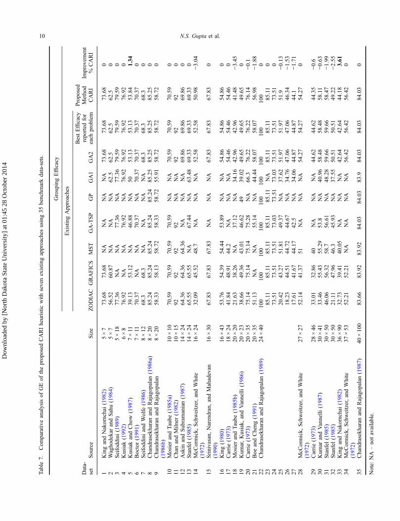
6. Results and discussion

Table 7 shows the details of comparative analysis of GE of the proposed CARI heuristic with seven existing approachesusing 35 benchmark data-sets gathered from the literature. Table 8 shows the comparative analysis of CARI heuristicwith some of the recent approaches to MPCF. The test was run on a personal computer with INTEL CORE i5 2.5 GHzprocessor. The size of the benchmark data-set used for assessing the performance of the proposed heuristic, ranges fromsmall (5 × 7) to large (40 × 100) and comprises well-structured as well as unstructured matrices. The proposed heuristicwas coded in MATLAB7.6. From Table 7, it can be observed that, for 22 data-sets (63%) CARI performed equally withGA2 and it performed better than GA2 for two data-sets (approximately 6%). CARI produced slightly lower results for11 data-sets (31%) in which, for four data-sets the deviation between the best result reported in the literature and the

Table 6. Machine-part cells.

International Journal of Production Research 9

Dow

nloa

ded

by [

Nor

th D

akot

a St

ate

Uni

vers

ity]

at 0

1:45

28

Oct

ober

201

4

Table

7.Com

parativ

eanalysisof

GEof

theprop

osed

CARIheuristic

with

sevenexistin

gapproaches

using35

benchm

arkdata-sets.

Data-

set

Sou

rce

Size

Group

ingEfficacy

ExistingApp

roaches

Propo

sed

Metho

dCARI

Improv

ement

%CARI

ZODIA

CGRAFICS

MST

GA-TSP

GP

GA1

GA2

BestEfficacy

repo

rted

for

each

prob

lem

1KingandNakornchai(198

2)5×7

73.68

73.68

NA

NA

NA

NA

73.68

73.68

73.68

02

Wagho

dekarandSahu(198

4)5×7

56.52

60.87

NA

NA

NA

62.5

62.5

62.5

62.5

03

Seifodd

ini(198

9)5×18

77.36

NA

NA

77.36

NA

77.36

79.59

79.59

79.59

04

Kusiak(199

2)6×8

76.92

NA

NA

76.92

NA

76.92

76.92

76.92

76.92

05

KusiakandCho

w(198

7)7×11

39.13

53.12

NA

46.88

NA

5053

.13

53.13

53.84

1.34

6Boctor(199

1)7×11

70.37

NA

NA

70.37

NA

70.37

70.37

70.37

70.37

07

Seifodd

iniandWolfe

(198

6)8×12

68.3

68.3

NA

NA

NA

NA

68.3

68.3

68.3

08

Chand

rasekh

aran

andRajagop

alan

(198

6a)

8×20

85.24

85.24

85.24

85.24

85.24

85.25

85.25

85.25

85.25

09

Chand

rasekh

aran

andRajagop

alan

(198

6b)

8×20

58.33

58.13

58.72

58.33

58.72

55.91

58.72

58.72

58.72

0

10MosierandTaube

(198

5a)

10×10

70.59

70.59

70.59

70.59

NA

NA

70.59

70.59

70.59

011

ChanandMiln

er(198

2)10

×15

9292

9292

NA

NA

9292

920

12Askin

andSub

ramanian(198

7)14

×24

64.36

64.36

64.36

NA

NA

NA

69.86

69.86

69.86

013

Stanfel

(198

5)14

×24

65.55

65.55

NA

67.44

NA

63.48

69.33

69.33

69.33

014

McC

ormick,

Schweitzer,andWhite

(197

2)16

×24

32.09

45.52

48.7

NA

NA

NA

52.58

52.58

50.98

−3.04

15Srinivasan,

Narendran,andMahadevan

(199

0)16

×30

67.83

67.83

67.83

NA

NA

NA

67.83

67.83

67.83

0

16King(198

0)16

×43

53.76

54.39

54.44

53.89

NA

NA

54.86

54.86

54.86

017

Carrie(197

3)18

×24

41.84

48.91

44.2

NA

NA

NA

54.46

54.46

54.46

018

MosierandTaube

(198

5b)

20×20

21.63

38.26

NA

37.12

NA

34.16

42.96

42.96

41.48

−3.45

19Kum

ar,Kusiak,

andVannelli

(198

6)20

×23

38.66

49.36

43.01

46.62

4939

.02

49.65

49.65

49.65

020

Carrie(197

3)20

×35

75.14

75.14

75.14

75.28

NA

66.3

76.22

76.22

76.14

−0.1

21Boe

andCheng

(199

1)20

×35

51.13

NA

NA

55.14

NA

44.44

58.07

58.07

56.98

−1.88

22Chand

rasekh

aran

andRajagop

alan

(198

9)24

×40

100

100

100

100

100

100

100

100

100

023

85.11

85.11

85.11

85.11

85.11

NA

85.11

85.11

85.11

024

73.51

73.51

73.51

73.03

73.51

73.03

73.51

73.51

73.51

025

20.42

43.27

51.81

49.37

NA

37.62

51.97

51.97

51.9

−0.13

2618

.23

44.51

44.72

44.67

NA

34.76

47.06

47.06

46.34

−1.53

2717

.61

41.67

44.17

42.5

NA

34.06

44.87

44.87

44.1

−1.71

28McC

ormick,

Schweitzer,andWhite

(197

2)27

×27

52.14

41.37

51NA

NA

NA

54.27

54.27

54.27

0

29Carrie(197

3)28

×46

33.01

32.86

40NA

NA

NA

44.62

44.62

44.35

−0.6

30Kum

arandVannelli

(198

7)30

×41

33.46

55.43

55.29

53.8

NA

40.96

58.48

58.48

58.11

−0.63

31Stanfel

(198

5)30

×50

46.06

56.32

58.7

56.61

NA

48.28

59.66

59.66

58.47

−1.99

32Stanfel

(198

5)30

×50

21.11

47.96

46.3

45.93

NA

37.55

50.51

50.51

49.22

−2.55

33KingandNakornchai(198

2)36

×90

32.73

39.41

40.05

NA

NA

NA

42.64

42.64

44.18

3.61

34McC

ormick,

Schweitzer,andWhite

(197

2)37

×53

52.21

52.21

NA

NA

NA

NA

56.42

56.42

56.42

0

35Chand

rasekh

aran

andRajagop

alan

(198

7)40

×10

083

.66

83.92

83.92

84.03

84.03

83.9

84.03

84.03

84.03

0

Note:

NA

–no

tavailable.

10 N.S. Gupta et al.

Dow

nloa

ded

by [

Nor

th D

akot

a St

ate

Uni

vers

ity]

at 0

1:45

28

Oct

ober

201

4

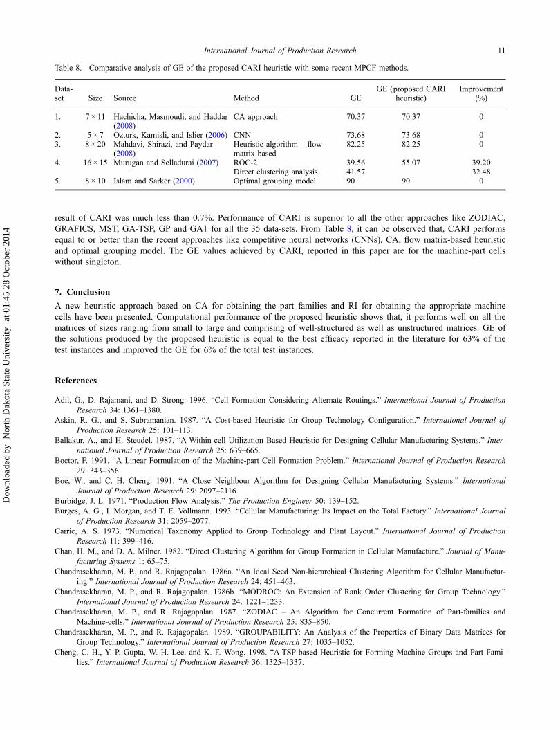
result of CARI was much less than 0.7%. Performance of CARI is superior to all the other approaches like ZODIAC,GRAFICS, MST, GA-TSP, GP and GA1 for all the 35 data-sets. From Table 8, it can be observed that, CARI performsequal to or better than the recent approaches like competitive neural networks (CNNs), CA, flow matrix-based heuristicand optimal grouping model. The GE values achieved by CARI, reported in this paper are for the machine-part cellswithout singleton.

7. Conclusion

A new heuristic approach based on CA for obtaining the part families and RI for obtaining the appropriate machinecells have been presented. Computational performance of the proposed heuristic shows that, it performs well on all thematrices of sizes ranging from small to large and comprising of well-structured as well as unstructured matrices. GE ofthe solutions produced by the proposed heuristic is equal to the best efficacy reported in the literature for 63% of thetest instances and improved the GE for 6% of the total test instances.

References

Adil, G., D. Rajamani, and D. Strong. 1996. “Cell Formation Considering Alternate Routings.” International Journal of ProductionResearch 34: 1361–1380.

Askin, R. G., and S. Subramanian. 1987. “A Cost-based Heuristic for Group Technology Configuration.” International Journal ofProduction Research 25: 101–113.

Ballakur, A., and H. Steudel. 1987. “A Within-cell Utilization Based Heuristic for Designing Cellular Manufacturing Systems.” Inter-national Journal of Production Research 25: 639–665.

Boctor, F. 1991. “A Linear Formulation of the Machine-part Cell Formation Problem.” International Journal of Production Research29: 343–356.

Boe, W., and C. H. Cheng. 1991. “A Close Neighbour Algorithm for Designing Cellular Manufacturing Systems.” InternationalJournal of Production Research 29: 2097–2116.

Burbidge, J. L. 1971. “Production Flow Analysis.” The Production Engineer 50: 139–152.Burges, A. G., I. Morgan, and T. E. Vollmann. 1993. “Cellular Manufacturing: Its Impact on the Total Factory.” International Journal

of Production Research 31: 2059–2077.Carrie, A. S. 1973. “Numerical Taxonomy Applied to Group Technology and Plant Layout.” International Journal of Production

Research 11: 399–416.Chan, H. M., and D. A. Milner. 1982. “Direct Clustering Algorithm for Group Formation in Cellular Manufacture.” Journal of Manu-

facturing Systems 1: 65–75.Chandrasekharan, M. P., and R. Rajagopalan. 1986a. “An Ideal Seed Non-hierarchical Clustering Algorithm for Cellular Manufactur-

ing.” International Journal of Production Research 24: 451–463.Chandrasekharan, M. P., and R. Rajagopalan. 1986b. “MODROC: An Extension of Rank Order Clustering for Group Technology.”

International Journal of Production Research 24: 1221–1233.Chandrasekharan, M. P., and R. Rajagopalan. 1987. “ZODIAC – An Algorithm for Concurrent Formation of Part-families and

Machine-cells.” International Journal of Production Research 25: 835–850.Chandrasekharan, M. P., and R. Rajagopalan. 1989. “GROUPABILITY: An Analysis of the Properties of Binary Data Matrices for

Group Technology.” International Journal of Production Research 27: 1035–1052.Cheng, C. H., Y. P. Gupta, W. H. Lee, and K. F. Wong. 1998. “A TSP-based Heuristic for Forming Machine Groups and Part Fami-

lies.” International Journal of Production Research 36: 1325–1337.

Table 8. Comparative analysis of GE of the proposed CARI heuristic with some recent MPCF methods.

Data-set Size Source Method GE

GE (proposed CARIheuristic)

Improvement(%)

1. 7 × 11 Hachicha, Masmoudi, and Haddar(2008)

CA approach 70.37 70.37 0

2. 5 × 7 Ozturk, Kamisli, and Islier (2006) CNN 73.68 73.68 03. 8 × 20 Mahdavi, Shirazi, and Paydar

(2008)Heuristic algorithm – flowmatrix based

82.25 82.25 0

4. 16 × 15 Murugan and Selladurai (2007) ROC-2 39.56 55.07 39.20Direct clustering analysis 41.57 32.48

5. 8 × 10 Islam and Sarker (2000) Optimal grouping model 90 90 0

International Journal of Production Research 11

Dow

nloa

ded

by [

Nor

th D

akot

a St

ate

Uni

vers

ity]

at 0

1:45

28

Oct

ober

201

4

Dimopoulos, C., and N. Mort. 2001. “A Hierarchical Clustering Methodology Based on Genetic Programming for the Solution ofSimple Cell-formation Problems.” International Journal of Production Research 39: 1–19.

George, A. P., C. Rajendran, and S. Ghosh. 2003. “An Analytical-iterative Clustering Algorithm for Cell Formation in Cellular Manu-facturing Systems with Ordinal-level and Ratio-level Data.” The International Journal of Advanced Manufacturing Technology22: 125–133.

Gonçalves, J. F., and M. G. C. Resende. 2004. “An Evolutionary Algorithm for Manufacturing Cell Formation.” Computers & Indus-trial Engineering 47: 247–273.

Gupta, N. S., and D. Devika. 2011. “A Novel Approach to Machine-part Cell Formation Using Mahalanobis Distance.” EuropeanJournal of Scientific Research 62 (1): 43–47.

Hachicha, Wafik, Faouzi Masmoudi, and Mohamed Haddar. 2008. “Formation of Machine Groups and Part Families in Cellular Man-ufacturing Systems Using a Correlation Analysis Approach.” The International Journal of Advanced Manufacturing Technology36: 1157–1169.

Hyer, N., and U. Wemmerlov. 1989. “Group Technology in the US Manufacturing Industry: A Survey of Current Practices.” Interna-tional Journal of Production Research 27: 1287–1304.

Islam, K. M. S., and B. R. Sarker. 2000. “A Similarity Coefficient Measure and Machine-parts Grouping in Cellular ManufacturingSystems.” International Journal of Production Research 38 (3): 699–720.

King, J. 1980. “Machine-component Grouping in Production Flow Analysis: An Approach Using a Rank Order Clustering Algo-rithm.” International Journal of Production Research 18: 213–232.

King, J., and V. Nakornchai. 1982. “Machine-component Group Formation in Group Technology: Review and Extension.” Interna-tional Journal of Production Research 20: 117–133.

Kumar, K., and M. P. Chandrasekaran. 1990. “Grouping Efficacy: A Quantitative Criterion for Goodness of Block Diagonal Forms ofBinary Matrices in Group Technology.” International Journal of Production Research 28 (2): 233–243.

Kumar, K. R., and A. Vannelli. 1987. “Strategic Subcontracting for Efficient Disaggregated Manufacturing.” International Journal ofProduction Research 25: 1715–1728.

Kumar, K. R., A. Kusiak, and A. Vannelli. 1986. “Grouping of Parts and Components in Flexible Manufacturing Systems.” EuropeanJournal of Operational Research 24: 387–397.

Kusiak, A. 1992. “Group Technology.” In Intelligent Design and Manufacturing, edited by A. Kusiak, 289–302. New York: Wiley.Kusiak, A., and W. Chow. 1987. “Efficient Solving of the Group Technology Problem.” Journal of Manufacturing Systems 6:

117–124.Mahdavi, Iraj, Babak Shirazi, and Mohammad Mahdi Paydar. 2008. “A Flow Matrix-based Heuristic Algorithm for Cell Formation

and Layout Design in Cellular Manufacturing System.” The International Journal of Advanced Manufacturing Technology 39:943–953.

McAuley, J. 1972. “Machine Grouping for Efficient Production.” Production Engineer 51: 53–57.McCormick, W. T., P. J. Schweitzer, and T. W. White. 1972. “Problem Decomposition and Data Reorganization by a Clustering Tech-

nique.” Operations Research 20: 993–1009.Megala, N., C. Rajendran, and R. Gopalan. 2008. “An Ant Colony Algorithm for Cell-formation in Cellular Manufacturing Systems.”

European Journal of Industrial Engineering 2: 298–336.Mosier, C. T., and L. Taube. 1985a. “The Facets of Group Technology and Their Impacts on Implementation – A State-of-the-art Sur-

vey.” Omega 13: 381–391.Mosier, C. T., and L. Taube. 1985b. “Weighted Similarity Measure Heuristics for the Group Technology Machine Clustering Prob-

lem.” Omega 13: 577–579.Murugan, M., and V. Selladurai. 2007. “Optimization and Implementation of Cellular Manufacturing System in a Pump Industry

Using Three Cell Formation Algorithms.” The International Journal of Advanced Manufacturing Technology 35 (1–2):135–149.

Nair, G. J., and T. T. Narendran. 1998. “CASE: A Clustering Algorithm for Cell Formation with Sequence Data.” International Jour-nal of Production Research 36: 157–180.

Onwubolu, G. C., and M. Mutingi. 2001. “A Genetic Algorithm Approach to Cellular Manufacturing Systems.” Computers & Indus-trial Engineering 39: 125–144.

Ozturk, Gurkan, Zehra Kamisli, and A. Attila Islier. 2006. “A Comparison of Competitive Neural Network with Other AI Techniquesin Manufacturing Cell Formation.” Lecture Notes in Computer Science 4221: 575–583.

Seifoddini, H. 1989. “Single Linkage versus Average Linkage Clustering in Machine Cells Formation Applications.” Computers &Industrial Engineering 16: 419–426.

Seifoddini, H., and P. Wolfe. 1986. “Application of the Similarity Coefficient Method in Group Technology.” IIE Transactions 18:271–277.

Srinivasan, G. 1994. “A Clustering Algorithm for Machine Cell Formation in Group Technology Using Minimum Spanning Trees.”International Journal of Production Research 32: 2149–2158.

Srinivasan, G., and T. T. Narendran. 1991. “GRAFICS – A Non-hierarchical Clustering Algorithm for Group Technology.” Interna-tional Journal of Production Research 29: 463–478.

12 N.S. Gupta et al.

Dow

nloa

ded

by [

Nor

th D

akot

a St

ate

Uni

vers

ity]

at 0

1:45

28

Oct

ober

201

4

Srinivasan, G., T. T. Narendran, and B. Mahadevan. 1990. “An Assignment Model for the Part-families Problem in Group Technol-ogy.” International Journal of Production Research 28: 145–152.

Stanfel, L. 1985. “Machine Clustering for Economic Production.” Engineering Costs and Production Economics 9: 73–81.Taguchi, Genichi, and Rajesh Jugulum. 2002. The Mahalanobis-Taguchi Strategy. New York: Wiley.Waghodekar, P. H., and S. Sahu. 1984. “Machine-component Cell Formation in Group Technology: MACE.” International Journal of

Production Research 22: 937–948.

International Journal of Production Research 13

Dow

nloa

ded

by [

Nor

th D

akot

a St

ate

Uni

vers

ity]

at 0

1:45

28

Oct

ober

201

4