The early universe

Carlo Baccigalupi

June 8, 2006

2

Contents

1 Introduction 51.1 Things to know for attending the course . . . . . . . . . . . . . . 51.2 Plan of the lectures . . . . . . . . . . . . . . . . . . . . . . . . . . 51.3 General relativity and quantum field theory . . . . . . . . . . . . 6

2 Cosmology with repulsive gravity 92.1 Comoving coordinates . . . . . . . . . . . . . . . . . . . . . . . . 10

2.1.1 Conformal time . . . . . . . . . . . . . . . . . . . . . . . . 112.2 Stress energy tensor . . . . . . . . . . . . . . . . . . . . . . . . . 112.3 Dynamics and conservation . . . . . . . . . . . . . . . . . . . . . 122.4 Cosmological species . . . . . . . . . . . . . . . . . . . . . . . . . 12

2.4.1 Relativistic and non-relativistic matter . . . . . . . . . . . 132.4.2 Cosmological constant . . . . . . . . . . . . . . . . . . . . 132.4.3 Scalar field . . . . . . . . . . . . . . . . . . . . . . . . . . 14

2.5 Cosmic acceleration . . . . . . . . . . . . . . . . . . . . . . . . . 14

3 Pre-inflationary cosmology 173.1 Thermal history of the universe . . . . . . . . . . . . . . . . . . . 173.2 Cosmological constant problem . . . . . . . . . . . . . . . . . . . 193.3 Flatness problem . . . . . . . . . . . . . . . . . . . . . . . . . . . 203.4 Horizon problem . . . . . . . . . . . . . . . . . . . . . . . . . . . 213.5 Inflationary kinematics . . . . . . . . . . . . . . . . . . . . . . . . 21

4 Inflationary cosmology 254.1 Scalar fields in cosmology . . . . . . . . . . . . . . . . . . . . . . 254.2 Inflation from scalar fields . . . . . . . . . . . . . . . . . . . . . . 26

4.2.1 Slow rolling . . . . . . . . . . . . . . . . . . . . . . . . . . 274.2.2 Inflationary models . . . . . . . . . . . . . . . . . . . . . . 284.2.3 Inflation as an attractor . . . . . . . . . . . . . . . . . . . 304.2.4 Re-heating at the end of inflation . . . . . . . . . . . . . . 32

5 Inflationary perturbations 355.1 Quantum fields in curved spacetime . . . . . . . . . . . . . . . . 35

6 Testing inflation 37

7 Cosmic acceleration today: the dark energy 39

3

4 CONTENTS

Chapter 1

Introduction

The aim of these lectures is to give an overview of the physics of the earlyuniverse, in the context of the inflationary cosmology. At the end of the course,a student should be able to understand most of the modern scientific papers onthis matter, ranging from the theoretical details of quantum fields in cosmology,down to the physical content and implications of the current experimental data.In this chapter, we give an overview of the course, specifying the most importantliterature to look at, as well as reviewing the plan of the lectures. In the end,we also fix the notation we adopt, and introduce very basic elements of generalrelativity and field theory.

1.1 Things to know for attending the course

These lectures aim at being self consistent, although some knowledge of generalrelativity and field theory is necessary in order to apprach them properly. More-over, who’s attending might benefit from having familiarity with the physics ofthe Friedmann Robertson Walker (FRW) background cosmology, as well as anyknowledge of cosmological perturbations.The main text where studying while attending the lectures should be repre-sented by the present notes. The students are on the other hand welcome toconsult the books and papers from where these notes have been taken. Theyare:

• textbook by Andrew R. Liddle and David H. Lyth, Cosmological Inflationand Large Scale Structure, Cambridge Press 2000,

• review paper by Hideo Kodama and Misao Sasaki, Progresses of Theoret-ical Physics Supplement 78, 1, 1984.

1.2 Plan of the lectures

The first part of the course contains a summary of the FRW cosmological back-ground, focusing on the expansion dynamics and in particular on the cosmicacceleration. This initial part sets the notation of the course and grants also acontinuity with possible previous courses that the students may have attended.The lectures then cover the following topics:

5

6 CHAPTER 1. INTRODUCTION

• pre-inflationary cosmology,

• kinematic of inflation,

• scalar fields in cosmology,

• inflationary models,

• the origin of cosmological perturbations,

• testing inflation with cosmic microwave background anisotropies,

• inflation and dark energy.

1.3 General relativity and quantum field theory

Spacetime is described by three spatial dimensions plus the time coordinate.Greek indeces run from 0 to 3, while latin indeces are used for spatial direc-tions, from 1 to 3. We use x to indicate a generic spacetime point, ~x and x forits spatial component and versor, respectively. The fundamental constants weuse are the Planck, Boltzmann and gravitational ones, indicated with h, kB andG, respectively. Unless specified otherwise, we work with unitary light speedvelocity, c = 1.Fields are function of the spacetime point x, and under coordinate transforma-tion they may behave as scalars, vectors or tensors if they have zero, one ormore than one Lorentz indeces, respectively. A tensor with two indeces, indi-cated with gµν(x) and called metric tensor, sets the infinitesimal distance fromtwo spacetime points, defined as

ds2 = gµνdxµdxν , (1.1)

where repeated indeces are summed. By an appropriate change on referenceframe, it is always possible to reduce the metric tensor to the Minkowski one,meaning that the system changes to the one which in free fall locally in x. Thesignature of the metric tensor we adopt is the following:

(−,+,+,+) . (1.2)

The inverse of the metric tensor is represented with the indeces up:

gµρgρν = δνµ , (1.3)

where δνµ is the Kronecker delta. We shall use the Kronecker delta in arbitraryindex configuration:

δνµ = δµν = δµν = 1 if µ = ν, 0 otherwise. (1.4)

The Christoffel symbols are defined as usual as

Γαβγ =12

(∂gαγ∂xβ

+∂gγβ∂xα

− ∂gαβ∂xγ

),

Γαβγ =12gαα

′(∂gα′β∂xγ

+∂gα′γ∂xβ

− ∂gβγ∂xα′

). (1.5)

1.3. GENERAL RELATIVITY AND QUANTUM FIELD THEORY 7

The Riemann, Ricci and Einstein tensors are given by

Rαβµν =∂Γαβν∂xµ

− ∂Γαβµ∂xν

+ ΓαλµΓλβν − ΓαλνΓ

λβµ , (1.6)

Rµν = Rααµν , (1.7)

andGµν = Rµν − 1

2gµνR , (1.8)

where R = Rµµ is the Ricci scalar.To simplify the notation, let us introduce the following conventions for derivationin general relativity:

• ;µ ≡ ∇µ means covariant derivative with respect to xµ,

• |a ≡ s∇a means covariant derivative with respect to the spatial metric,i.e. the 3× 3 array obtained removing the time column and row from themetric tensor in (1.1),

• ,µ means ordinary derivative with respect to xµ .

A vector, vµ can be obtained via covariant derivation of a scalar quantity s as

vµ = s;µ = s,µ , (1.9)

where the last equality holds for scalars only. A tensor can be obtained viacovariant derivation of a vector as

tµν = vµ;ν = vµ,ν − vαΓαµν . (1.10)

Covariant derivative raise further the rank of tensors as

uµνρ = tµν;ρ = tµν,ρ − tανΓαµρ − tµαΓαρνuνµρ = tνµ;ρ = tνµ,ρ − tναΓαµρ + tαµΓνρα , (1.11)

and the process of course is not limited in the number of Lorentz indeces.Field quantization is performed conveniently in the Fourier space. For a real

scalar field ψ(x) with mass m it reads

ψ =∫

d3p

(2π)31√2E~p

[a~pu(~p)ei~p·~x + a+

~p u∗(~p)e−i~p·~x

], (1.12)

where a~p and its Hermitian conjugate a+~p are the annihilation and creation op-

erators of a quantum with momentum ~p, with energy E~p =√m2 + ~p2. The

vacuum state in the Fock space is indicated as usual as |0 >. The u~pei~p·~x func-tion and its complex conjugate u∗(~p)e−i~p·~x are eigenfunctions of the Hamiltonianof the system; for a massless and non-interacting field, u(~p)ei~p·~x = ei(−|~p|t+~p·~x)

The commutation relations are

[ψ(x), ψ+(x′)] = ihδ3(~x− ~x′) , (1.13)

related as usual to the space coordinate only.

8 CHAPTER 1. INTRODUCTION

Chapter 2

Cosmology with repulsivegravity

In this chapter we review the main aspects of the FRW cosmology, focusingon the species which may induce a repulsive gravity effect, appearing as anaccelerated cosmic expansion.

The FRW metric is built upon the hypothesis that space is homogeneousand isotropic at all times. The first condition means that at a given time, thephysical properties, e.g. expansion rate, particle density etc., are the same ineach point. The second condition means that any physical observable does notdepend on the direction of an observer located in any spacetime point x.These assumptions simplify dramatically the structure of the metric tensor gµν .A spherical symmetry around each spacetime location is necessary, so that nooff-diagonal terms are left; homegeneity and isotropy leave essentially only twodegrees of freedom to the system. The first one is a global scale factor, fixingat each time the value of physical lengths. The second one is related to thespacetime curvature, as an homogeneous metric can be globally more or lesscurved. The form of the fundamental length element is therefore

ds2 = −dt2 + a(t)2(

11−Kr2

dr2 + r2dθ2 + r2 sin2 θdφ2

), (2.1)

where a(t) and K represent the global scale factor and the curvature, respec-tively; r, θ and φ are the usual spherical coordinates for radius, polar and azimutangle, respectively.The physical meaning of the scale factor can be read straightforwardly from themetric, and the only point to discuss concerns its dimension. One may assignphysical dimensions to the scale factor a or to the radial coordinate r; in thislectures, we choose the second option. Concerning the curvature, some morediscussion is needed. The first point is about dimensions again; if r is dimen-sionless, K is also dimensionless. If r is a length, then K is the inverse of thesquare of a length. Moreover, if K = 0, then the spatial part of the length (2.1)is Minkowskian, and in this case the FRW metric is flat. If K > 0, there isan horizon in the metric, given by rH = ±1/

√K; this means that an infinite

physical distance corresponds to those coordinates, regardless of the value of thescale factor a, and the FRW metric is closed; note that this does not conflict

9

10 CHAPTER 2. COSMOLOGY WITH REPULSIVE GRAVITY

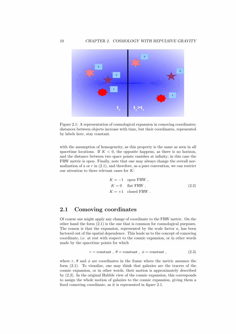
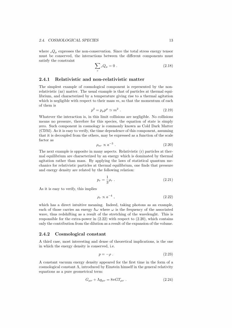
Figure 2.1: A representation of cosmological expansion in comoving coordinates;distances between objects increase with time, but their coordinates, representedby labels here, stay constant.

with the assumption of homogeneity, as this property is the same as seen in allspacetime locations. If K < 0, the opposite happens, as there is no horizon,and the distance between two space points vanishes at infinity; in this case theFRW metric is open. Finally, note that one may always change the overall nor-malization of a or r in (2.1), and therefore, as a pure convention, we can restrictour attention to three relevant cases for K:

K = −1 open FRW ,

K = 0 flat FRW , (2.2)K = +1 closed FRW .

2.1 Comoving coordinates

Of course one might apply any change of coordinate to the FRW metric. On theother hand the form (2.1) is the one that is common for cosmological purposes.The reason is that the expansion, represented by the scale factor a, has beenfactored out of the spatial dependence. This leads us to the concept of comovingcoordinate, i.e. at rest with respect to the cosmic expansion, or in other wordsmade by the spacetime points for which

r = constant , θ = constant , φ = constant , (2.3)

where r, θ and φ are coordinates in the frame where the metric assumes theform (2.1). To visualize, one may think that galaxies are the tracers of thecosmic expansion, or in other words, their motion is approximately describedby (2.3). In the original Hubble view of the cosmic expansion, this correspondsto assign the whole motion of galaxies to the cosmic expansion, giving them afixed comoving coordinate, as it is represented in figure 2.1.

2.2. STRESS ENERGY TENSOR 11

2.1.1 Conformal time

Although time does not enter in the discussion about comoving coordinatesabove, there is a very common time variable which may replace the ordinarytime in (2.1). By performing the coordinate change

dτ =dt

a(t), (2.4)

the FRW metric may be easily written as

gµν ≡ a2 ·

−1 0 0 00 (1−Kr2)−1 0 00 0 r2 00 0 0 r2 sin2 θ

≡ a2γµν (2.5)

so that the cosmic expansion is completely factored out of the comoving partof the metric, which we define as γµν ; τ is the conformal time, and is ourtime variable in the following, unless otherwise specified. We will indicate theconformal time derivative with , while those with respect to the ordinary time areindicated with the subscript t. It is also useful to define two different quantitiesdescribing the velocity of the expansion, i.e.

H =ata

, H =a

a, (2.6)

named ordinary and conformal Hubble expansion rates, respectively; as it iseasy to see, the two are related by H = H/a.

2.2 Stress energy tensor

The stress energy tensor specifies the content of spacetime, in terms of physicalentities, i.e. particles, fields and their properties. We limit ourselves here todescribe a perfect relativistic fluid, homogeneous and isotropic. These assump-tions again restrict dramatically the complexity of the general expression forthe stress energy tensor. The quantities that characterize it are just the energydensity, ρ, and the pressure p. The quantities in the stress energy tensor whichhas direct physical meaning are those with covariant and controvariant indeces.In this form, T νµ is most easy as the (0, 0) components represent the energydensity, while p is isotropically assigned to all directions as

T νµ ≡

−ρ 0 0 00 p 0 00 0 p 00 0 0 p

, (2.7)

where the minus to the energy density is due to the choice of our signature (1.2).The stress energy tensor may also be written as

Tµν = (ρ+ p)uµuν + pgµν , (2.8)

where uµ represents the quadri-velocity of a fluid element, with an affine pa-rameter which for convenience may be taken as the conformal time itself:

uµ =dxµ

dτ. (2.9)

12 CHAPTER 2. COSMOLOGY WITH REPULSIVE GRAVITY

In analogy with the normalization of the quadri-impulse of a particle with massm, pµpµ = −m2, and since the energy is represented by the term ρ+ p in (2.9),the quadri-velocities are normalized as uµuµ = −1. In comoving coordinates,where the ua = 0, this condition implies

uµ ≡(

1a, 0, 0, 0

). (2.10)

2.3 Dynamics and conservation

The Einstein and conservation equations

Gµν = 8πGTµν , T ;νµν = 0 , (2.11)

reduce to two differential equations only, where the independent variable isthe time τ , expressing the dynamics of the expansion, plus the conservation ofenergy, respectively. The first one is the Friedmann equation

H2 =8πG

3a2ρ−K , (2.12)

which is equivalent to the equation ruling the acceleration of the expansion:

H − H2 = −4πGa2(ρ+ p) . (2.13)

The conservation equation becomes

ρ+ 3H(ρ+ p) = 0 . (2.14)

As it is evident, it is impossible to solve this system if some relation betweenpressue and energy density is given, p(ρ). For interesting cases, as those weshall see in the next Section, pressure is proportional to the energy density:

p = wρ , (2.15)

where w is the equation of state of the fluid, which may have a time dependenceas any other cosmological component in the FRW background.

2.4 Cosmological species

So far we did not consider the case in which the stress energy tensor is madeby more than one component, although in a realistic case, several of them arepresent at the same time. In this case, the stress energy tensor we treated so farcorresponds to the total one, a sum over those corresponding to each component,labeled by c as follows:

Tµν =∑c

cTµν . (2.16)

The single stress energy tensors may not be conserved as a result of mutual inter-actions between the different components. Therefore, the conservation equationfor each component may be written as

cT;νµν = cQµ , (2.17)

2.4. COSMOLOGICAL SPECIES 13

where sQµ expresses the non-conservation. Since the total stress energy tensormust be conserved, the interactions between the different components mustsatisfy the constraint ∑

c

cQµ = 0 . (2.18)

2.4.1 Relativistic and non-relativistic matter

The simplest example of cosmological component is represented by the non-relativistic (nr) matter. The usual example is that of particles at thermal equi-librium, and characterized by a temperature giving rise to a thermal agitationwhich is negligible with respect to their mass m, so that the momentum of eachof them is

p2 = pµpµ ' m2 . (2.19)

Whatever the interaction is, in this limit collisions are negligible. No collisionsmeans no pressure, therefore for this species, the equation of state is simplyzero. Such component in cosmology is commonly known as Cold Dark Matter(CDM). As it is easy to verify, the time dependence of this component, assumingthat it is decoupled from the others, may be expressed as a function of the scalefactor as

ρnr ∝ a−3 . (2.20)

The next example is opposite in many aspects. Relativistic (r) particles at ther-mal equilibrium are characterized by an energy which is dominated by thermalagitation rather than mass. By applying the laws of statistical quantum me-chanics for relativistic particles at thermal equilibrium, one finds that pressureand energy density are related by the following relation:

pr =13ρr . (2.21)

As it is easy to verify, this implies

ρr ∝ a−4 , (2.22)

which has a direct intuitive meaning. Indeed, taking photons as an example,each of those carries an energy hω where ω is the frequency of the associatedwave, thus redshifting as a result of the stretching of the wavelenght. This isresponsible for the extra-power in (2.22) with respect to (2.20), which containsonly the contribution from the dilution as a result of the expansion of the volume.

2.4.2 Cosmological constant

A third case, most interesting and dense of theoretical implications, is the onein which the energy density is conserved, i.e.

p = −ρ . (2.23)

A constant vacuum energy density appeared for the first time in the form of acosmological constant Λ, introduced by Einstein himself in the general relativityequations as a pure geometrical term:

Gµν + Λgµν = 8πGTµν . (2.24)

14 CHAPTER 2. COSMOLOGY WITH REPULSIVE GRAVITY

Indeed, bringing it to the right hand side, and passing to the mixed form forthe indeces, one gets

Gνµ = 8πG(T νµ −

Λ8πG

δνµ

), (2.25)

and looking at the form of the stress energy tensor (1.10) it is straightforwardto verify that the one related to the cosmological constant is characterized bypΛ = −ρΛ = −Λ/8πG.

2.4.3 Scalar field

The simplest generalization of a constant energy density is represented by ascalar field Ψ. Its stress energy tensor may be obtained by varying the actionin general relativity with respect to the metric in order to get the Einsteinequations. The Lagrangian density for a scalar field ψ in general relativity isgiven by

L =R

16πG+ ψ;µψ

;µ − V (ψ) , (2.26)

where V represents the potential energy. The variation with respect to themetric leads to the following expression for the scalar field stress energy tensor:

Tµν = ψ;µψ;nu +(

12ψ;ρψ

;ρ − V

)gµν . (2.27)

In a FRW background, the field may depend on the time coordinate only. Bylooking at the expression above in the FRW limit, one may easily see that thescalar field is equivalent to a fluid which has an energy density

ρ =1

2a2ψ2 + V , (2.28)

and a pressure given by

p =1

2a2ψ2 − V , (2.29)

Interestingly, the scalar field reduces to the case of a cosmological constant inthe limit ψ = 0.

2.5 Cosmic acceleration

We close this chapter by pointing out which one among the cosmological speciesmentioned above is able to induce an accelerated cosmic expansion. The lattercondition is simply equivalent to

a > 0. (2.30)

From (2.13), using (2.12), it is immediately evident that

atta

= −4πG3

(ρ+ 3p)− K

a2. (2.31)

2.5. COSMIC ACCELERATION 15

The first thing to note is that an open universe, with K < 0, contributes tomake att > 0. The second thing to note is that in order to have accelerationfrom the content of the stress energy tensor, one must have

w < −13. (2.32)

If the energy density is positive, that means that the pressure must be negativeas in the case of the cosmological constant, or the scalar field with vanishingkinetic energy.

16 CHAPTER 2. COSMOLOGY WITH REPULSIVE GRAVITY

Chapter 3

Pre-inflationary cosmology

In this chapter we review the main aspects of cosmology as it was before theintroduction of the concept of inflation, focusing on the problems of the wholepicture and showing how a phase of exponential expansion in the early universemay constitute an elegant solution.

3.1 Thermal history of the universe

The cosmic microwave background represents a very strong indication that theuniverse was hotter in its early stages. Today the non-relativistic component ofthe energy density, which we indicate generically as matter, is about 25% of thetotal one; photons and neutrinos, which are relativistic and indicated genericallyas radiation, are about 100000 times less abundant. Given that matter scalesas the inverse of the cube of the scale factor, while radiation as the inverse ofthe fourth power, it is easy to calculate that the moment at which matter andradiation were comparable occurs at an epoch corresponding to

1 + zeq =a0

aeq' 104 , (3.1)

where z = a0/aeq−1 is the redshift coordinate, eq marks the equivalence epoch,and a0 represents the value of the scale factor at the present, which we assume tobe 1 in the following. Given that the CMB temperature scales as the inverse ofthe scale factor, and that today it is about 2.726 Kelvin, the equivalence epochcorresponds to about 3 · 104 Kelvin. At that temperature, CMB and photonsare tightly coupled via Thomson scattering. That means that the mean freepath, simply related to the number density of targets and the Thomson crosssection, is typically much smaller than the causal scale associated to the cosmicexpansion, which corresponds to the inverse of the Hubble length:

λT = 1/(neσT ) ¿ H−1 . (3.2)

In this regime, photons are tightly coupled with all charged particles, so that asingle temperature characterizes the whole system. Going back in time, densitiesincrease for all species, and sooner or later all interactions occur on spacetimescales smaller than the horizon, no matter how small is the cross section.

17

18 CHAPTER 3. PRE-INFLATIONARY COSMOLOGY

In other words, the early universe is characterized by a single temperature de-scribing a thermal bath of elementary bosons and fermions tightly coupled bytheir interactions. Is this picture going to persist at any time, no matter howearly it is?There is a natural limit at which this picture cannot be trusted. The currentmodel of particle physics predicts unification of the different interactions athigh energy. An example is represented by the electromagnetic and weak inter-actions, which are thought to decouple via a spontaneous symmetry breakingat an energy scale comparable to the mass of the particle responsible for thatbreaking, the Higgs boson, corresponding to a few hundreds of GeV. In unitsof temperature, 102 GeV is equivalent to about 1015 K. This scale more or lessrepresents the limits of the physics we can probe directly in laboratories.Let us review the most important steps in the thermal cosmic history, goingbackward in time, up to that scale:

• E = kBT ' 10−1 eV, photon baryon decoupling,

• E ' 100 eV, matter radiation equality,

• E ' 10−1 MeV, nucleosynthesis through deuterium formation from neu-tron proton scattering,

• E ' 100 MeV, neutrino decoupling from neutrino antineutrino annihlila-tion in electron positron pairs, electron positron annihilation in two pho-tons,

• E ' 102 GeV, symmetry breaking between electromagnetic and weakinteraction,

• ...?

At higher energies or at earlier cosmological epochs, the electromagnetic andweak interactions should be described by a single one, named electroweak. Sim-ilar models exist for the unification of the strong interaction with the others,which should occur at earlier cosmological epochs. It is conceivable that also thegravitational interaction unifies with the other forces; although there is not asuccessful model for that, one may guess that such epoch corresponds to the en-ergy scale which may be formed combining the fundamental constant includingthe gravitational one:

EPlanck =

√hc5

G' 1019 GeV . (3.3)

In the above expression, we have momentarily re-introduced the use of the speedof light constant, c, keeping that until the end of this section. If this is indeed thescale at which gravity unifies with other forces, then a large gaps seperates thisscale from the highest one which may be probed directly in laboratories on theEarth, which is about 102 GeV. The time coordinate which may be associatedto the fundamental constant, including G, is given by

tPlanck =

√hG

c5' 10−55 s , LPlanck = c · tPlanck =

√hG

c3' 10−35 cm . (3.4)

3.2. COSMOLOGICAL CONSTANT PROBLEM 19

The relations (3.3) and (3.4) may be combined to obtain the Planck energydensity, which is

ρPlanck =EPlanckL3Planck

' 10123ρ0 , (3.5)

where ρ0 = 3(cH0)2/8πG is the present critical energy density, correspondingto about 10−8 g/cm3.The Planck energy scale represents the limit for our understanding of cosmology,but also for physics as a whole. At this epoch, the physics of spacetime andparticles can no longer be thought as decoupled. Since no viable prediction forthe physics at this energy has been produced, at the moment this is the borderbetween physical investigations and speculations.

3.2 Cosmological constant problem

Historically, there are two ways in which a constant vacuum energy appearedin the Einstein equations:

Gµν + Λgµν = 8πG(Tµν + V gµν) . (3.6)

The first term is the cosmological constant, which we have already seen, intro-duced by Einstein in 1916. Its conception is entirely geometric. He removed itfrom the general relativity equations, when he realized that it was not capableof keeping the universe static, as he thought in the beginning. In the FRWcosmology, that is easily seen by noting that the Friedmann equation reduces toH2 = constant, which admits an exponential expansion as a solution. Later on,the case for a constant energy density in the vacuum was raised independentlyby quantum mechanics, and is represented by V in the equation above; essen-tially, there is no reason why quantum systems should have the fundamentalstate at zero energy, and in many cases actually they assign a non-zero energyto it. The simplest example is that of the harmonic oscillator at frequency ω,which has the following energetic levels:

En =(n+

12

)hω . (3.7)

The fundamental state at n = 0 does possess a non-zero energy. Let us lookat the expectations that we may have for Λ and V in (3.6). Basically, thereis no expectation at all for Λ. There is no theory for V , but there is theexpectation that it is of the order of the Planck energy density, for the followingreasons. As we have already stressed, the current hypothesis on the physicalprocesses at high energies do predict the unification of physical interactions.The highest one, involving all interactions including gravity, corresponds to thePlanck energy density. Since quantum mechanics generically predicts a vacuumenergy density, it is reasonable to expect that it is of the order of the Planckenergy density itself.Whatever are the values of Λ and V , the cosmological constant problem isthat they are required to cancel out with a fantastic precision, simply becausethe vacuum energy density today can at most be comparable with the presentcritical energy density in order to be compatible with the recent cosmological

20 CHAPTER 3. PRE-INFLATIONARY COSMOLOGY

history; from (3.5) one gets

|Λ/8πG− V |ρPlanck

<∼ 10−123 . (3.8)

This problem has been there for almost a century now, and the evidence forcosmic acceleration, saying that the number above is actually different fromzero and of the order of 10−123, renewed the interest in it. Since inflationand the models of the early universe deal with an early stage of cosmologicalexpansion which is dominated by some sort of vacuum energy, it is appropriateto mention it here. On the other hand, no model of the early universe, or ingeneral no physical argument has been able to exmplain it so far.

3.3 Flatness problem

In the scenario we have been treating so far, the cosmological expansion isdominated by radiation at arbitrarily small times. This caused several problemsconnected with the dynamics of the cosmic expansion. The first one is knownas the flatness problem, which we describe here.Indicating with ρc = 3H2/8πG the critical density at an arbitrary time, let usconsider the quantity

∣∣∣∣ρ

ρc− 1

∣∣∣∣ = |Ω− 1| = 1a2H2

. (3.9)

where the last equality is taken from the Friedmann equation (2.12), takinginto account that by rescaling the coordinates, it is always possible to deal withvalues of the curvature K equal to 0, ±1. The present data in cosmology saythat the universe is close to flatness, i.e.

|Ω− 1|0 = O(10−2) . (3.10)

Let us see how this number goes back in time. From the known scaling ofmatter and radiation energy densities, it is easy to see that the scaling of H inthe matter and radiation dominated eras (MDE, RDE) are

H ∝ a−3/2 in the MDE ,H ∝ a−2 in the RDE . (3.11)

By assuming that the universe is matter dominated after equivalence and radi-ation dominated before, at an arbitrary epoch during the RDE, one has

|Ω− 1| = a2

a2eq

|Ω− 1|eq =a2

a2eq

a3/2eq

a3/20

|Ω− 1|0 . (3.12)

The ratios between the scale factors at different epochs may be calculated byusing again the energy scale, proportional to the temperature and inverselyproportional to the scale factor. The second ratio in (3.12) yields a factor(10−4)3/2 = 10−6. If we compute the first ratio at the Planck scale (3.3), theresult is

|Ω− 1|Planck = 10−62|Ω− 1|0 . (3.13)

That means that if |Ω − 1|0 today is different from zero, then one must haveadjusted the initial energy density to be extremely close to the critical one,in order to yield the value observed at present. Other than that, there is noexplanation for this problem in the present scenario.

3.4. HORIZON PROBLEM 21

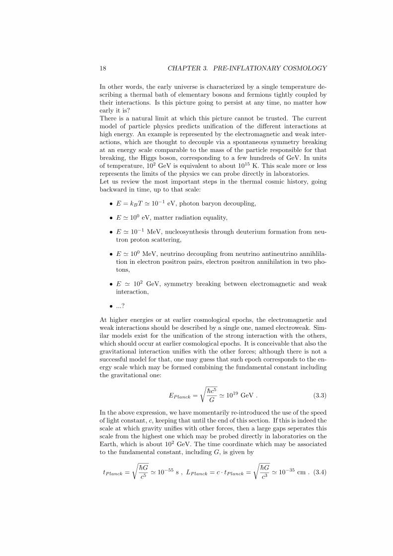
Figure 3.1: A representation of the behavior of horizon and scales as a functionof the scale factor, in a logarithmic scale.

3.4 Horizon problem

In figure 3.1 we show the behavior of horizon and physical scales as a functionof the scale factor, on a logarithmic scale. The scaling of the Hubble horizonhas been taken from (3.11). Physical scales scale of course linearly with a.As it is evident, for any physical scale λ there is only one epoch at which itequals the Hubble horizon, i.e. one moment only in which it is in horizoncrossing. After that epoch, a perturbation on that scale is always within thehorizon, thus capable to thermalize. Before that epoch, no causal connectionexists for structures separated by that scale. The horizon problem comes whenone considers in particular the scale λ which is entering the horizon today. Onthat scale, we see a remarkable isotropy represented by the temperature of theCMB, which is the same with corrections of one part over 105 on all scales. Fromthe elementary reasoning in the figure, we also know that that scale was neverin causal connection in the past, at least in the present scheme. The horizonproblem asks for an explanation of this level of isotropy on super-horizon scales,which in the present scheme where the RDE goes on indefinitely in the past,may be explained only if someone put by hands an extremely high level ofhomogeneity in the perturbations in the early universe.

3.5 Inflationary kinematics

We condlude this chapter showing how an era of accelerated expansion whichoccurs before the RDE may solve at least the last two of the problems mentionedabove.Suppose indeed that the cosmological expansion history is described by the rep-resentation in figure 3.2, in which the RDE comes after and era in which His a constant; in an FRW cosmology, that is achieved by having a cosmologi-cal constant, regardless of the cosmological curvature. Indeed, if K = 0, the

22 CHAPTER 3. PRE-INFLATIONARY COSMOLOGY

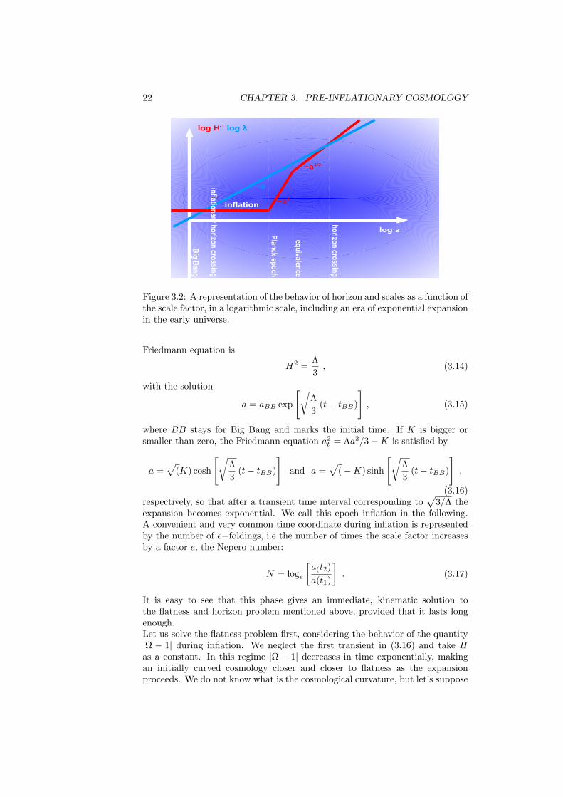
Figure 3.2: A representation of the behavior of horizon and scales as a function ofthe scale factor, in a logarithmic scale, including an era of exponential expansionin the early universe.

Friedmann equation is

H2 =Λ3, (3.14)

with the solution

a = aBB exp

[√Λ3

(t− tBB)

], (3.15)

where BB stays for Big Bang and marks the initial time. If K is bigger orsmaller than zero, the Friedmann equation a2

t = Λa2/3−K is satisfied by

a =√

(K) cosh

[√Λ3

(t− tBB)

]and a =

√(−K) sinh

[√Λ3

(t− tBB)

],

(3.16)respectively, so that after a transient time interval corresponding to

√3/Λ the

expansion becomes exponential. We call this epoch inflation in the following.A convenient and very common time coordinate during inflation is representedby the number of e−foldings, i.e the number of times the scale factor increasesby a factor e, the Nepero number:

N = loge

[a(t2)a(t1)

]. (3.17)

It is easy to see that this phase gives an immediate, kinematic solution tothe flatness and horizon problem mentioned above, provided that it lasts longenough.Let us solve the flatness problem first, considering the behavior of the quantity|Ω − 1| during inflation. We neglect the first transient in (3.16) and take Has a constant. In this regime |Ω − 1| decreases in time exponentially, makingan initially curved cosmology closer and closer to flatness as the expansionproceeds. We do not know what is the cosmological curvature, but let’s suppose

3.5. INFLATIONARY KINEMATICS 23

that cosmology at the beginning is represented by some value |Ω−1|BB differentfrom zero. We may as how long the inflation has to last, in order to match thevalue at the Planck epoch which we extrapolate from the present, in (3.13). Itis easy to see that the latter condition implies

|Ω− 1|Planck = |Ω− 1|BB(

aBBaPlanck

)2

= 10−62|Ω− 1|0 . (3.18)

By giving to the last quantity the present upper limit, |Ω−1|0 <∼ 10−2, one gets

aPlanckaBB

=√

1064|Ω− 1|BB . (3.19)

If one assumes that initially the cosmological curvature and energy densityyielded comparable terms, represented by |Ω − 1|BB = O(1), a solution to theflatness problem is achieved if inflation lasts for about 74 e−foldings at least.Let us now consider the horizon problem. Rejecting the hypothesis of an exter-nal intervention setting the initial conditions on super-horizon scales, the wholeuniverse we see today must have been within the Hubble horizon in the past, inorder to thermalize and reach the remarkable level of homogeneity we see todaythrough the CMB. As it is evident in figure 3.2, inflation gives you an easysolution to this problem, provided again that it lasts long enough so that thecosmological scale corresponding to the observed universe today was inside thehorizon after the Big Bang. The scale of the observed universe today is abouttwice to the present value of the Hubble horizon, which is about 8200 Mpc. Theepoch of the horizon crossing during inflation is obtained by matching that scalewith H−1 during inflation, which constant and therefore equal to the value ithas at the Planck epoch, H−1

Planck. This leads to the condition

2H−10 · aIHC

a0= H−1

Planck , (3.20)

where IHC indicates the inflationary horizon crossing. By using the knownscaling in the MDE and RDE up to the Planck epoch, it is easy to see thatH−1Planck = (aPlanck/aeq)2(aeq/a0)3/2H−1

0 ' 10−60H−10 . Moreover, aIHC/a0 =

(aIHC/aPlanck) · (aPlanck/a0) ' 10−31(aIHC/aPlanck). Thus the relation (3.20)becomes

2aIHCaPlanck

= 10−29 , (3.21)

which implies that inflation must have lasted for about 67 e−foldings at leastin order to have the whole universe we see today in horizon crossing duringinflation itself.

The solution to the flatness and horizon problems is due essentially to theexponentially accelerated cosmological expansion, which goes like under theeffect of a repulsive gravity, radically different from the behavior induced bythe ordinary particles in the RDE and MDE. This tells that the kinematic ofinflation is very promising in solving at least two of the three classical problemsof the pre-inflationary FRW cosmology. This motivated the construction ofsome physical models for this process, to be treated in the next chapter.

24 CHAPTER 3. PRE-INFLATIONARY COSMOLOGY

Chapter 4

Inflationary cosmology

In this chapter we review the simplest inflationary models, focusing on thebehavior of the background expansion. We first give the basics of scalar fieldphysics in the context of cosmology, then give the conditions for having a viableinflationary epoch out of a scalar field model, and finally we treat some specificmodel in some detail.

4.1 Scalar fields in cosmology

A dynamical quantity q of a point-like object moving under the effect of apotential V (q) is described by the action

S =∫ +∞

−∞Ldt =

∫ +∞

−∞

[12q2t − V (q)

]dt , (4.1)

where L represents the Lagrangian of the system. The motion equation corre-spond to the trajectories q(t) which extremize the action above:

d

dt

∂L

∂qt+ Vq = 0 ⇔ qtt + Vq = 0 . (4.2)

In field theory, the system above represents the global limit of a local theory, inwhich the degrees of freedom are different in any spacetime point:

q(t) → ψ(x) . (4.3)

If ψ is constrained to be homogeneous in space, i.e. in the coordinates ~x, fieldtheory reduces to the physical system above. Correspondingly, the action mustbe generalized to

S =∫ +∞

−∞L√−gd4x , (4.4)

where the integration is over the whole spacetime now, and the term√−g with

g indicating the metric tensor determinant is necessary to make S a generalrelativistic invariant. The Lagrangian becomes a Lagrangian density, where thefield dependence on all coordinates is made manifest by the covariant derivativesinstead than on time only; the potential V (ψ) still rules the dynamics, and if the

25

26 CHAPTER 4. INFLATIONARY COSMOLOGY

argument of the potential is the field only, the field is self-interacting. moreover,the Lagrangian of gravity in general relativity is the scalar quantity R/16πG.Thus, the dynamics of a self-gravitating and self-interacting scalar fiels is givenby

L =R

16πG+

12ψµψ

µ − V (ψ) . (4.5)

The motion equations again correspond to the trajectories extremizing the ac-tion. We have now a double dynamics, induced separately by gravity and thescalar field. The extremization with respect to the metric gives the Einsteinfield equations

∂L∂gµν

− 12gµνL = 0 ⇔ Gµν = 8πGTµν , (4.6)

where

ψTµν = ψ;µψ;ν − gµν

[12ψ;ρψ

;ρ + V (ψ)]. (4.7)

Similarly, the extremization with respect to the scalar field trajectories give theKlein-Gordon equation

(∂L∂ψµ

)

;µ

+∂V

∂ψ⇔ ψ;µ

;mu + Vψ = 0 , (4.8)

where = ψ;µ;µ . The latter equation coincides with the conservation equation

(ψT νµ );ν = 0.The FRW limit of the present picture nicely reduces to a system as simple asthe one we described in the beginning of this section. The dependence on ~xdisappears and the Klein-Gordon equation becomes

ψtt + 3Hψt + Vψ = 0 , (4.9)

where with respect to (4.2) we notice effect of gravity, through a cosmologicalfriction equal to the number of spatial dimensions multiplied by the Hubbleexpansion rate. The latter also corresponds to the continuity equation ρψtt +3H(ρψ + pψ), where

ρψ =12ψ2t + V (ψ) (4.10)

pψ =12ψ2t − V (ψ) . (4.11)

The Friedmann equation is therefore

H2 =8πG

3ρφ +

K

a2=

8πG3

[12ψ2t + V (ψ)

]+K

a2. (4.12)

4.2 Inflation from scalar fields

It is clear that in the limit of a static field, ψt → 0, the system of equationsabove reduces to the one of a cosmological constant, where the latter is simplythe scalar field potential V . The whole idea of inflation from a scalar field, namedthe inflaton, is that the latter enters a low dynamic phase in which the potentialenergy V > 0 plays the role of a slowly dynamical cosmological constant; this

4.2. INFLATION FROM SCALAR FIELDS 27

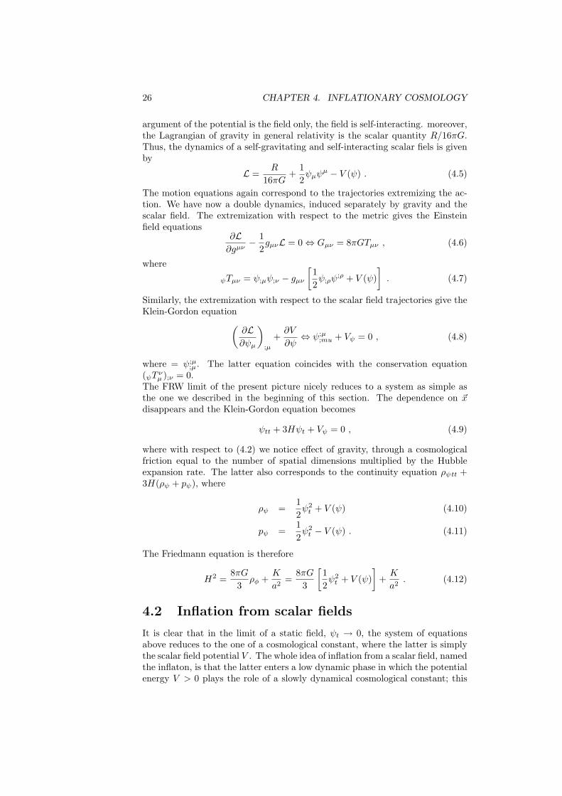
Figure 4.1: The simplest picture of an inflationary model.

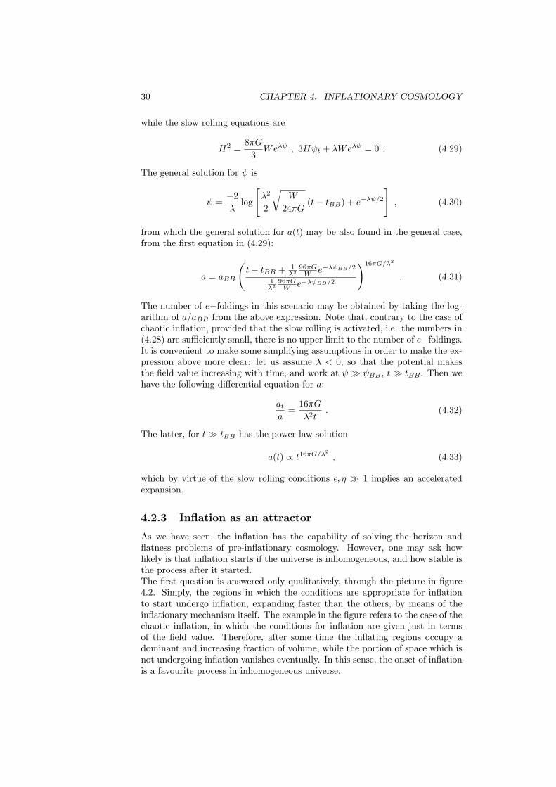
phase must last long enough to inflate the space as needed to solve the horizonand flatness problems mentioned in the previous chapter. This mechanism isquite natural in a shallow potential V with a global minimum, as representedin figure 4.1. In this picture, the field value ψ undergoes a slow rolling on thepotential, activating the inflationary expansion which ends when it reaches theminimum.

4.2.1 Slow rolling

The concept of slow rolling is actually common to most of the inflationarymodels proposed so far, and may be casted as a requirement to the shape ofthe potential in order to be able to activate the inflationary expansion for anamount of time which is enough to solve the horizon and flatness problems. If ascalar field ψ is the only cosmological component obeying the dynamics imposedby the potential energy density V , the Friedmann and Klein Gordon equationsare

H2 =8πG

3

(12ψ2t + V

)+K

a2, ψtt + 3Hψt + Vψ = 0 (4.13)

and complete the description of the system. In order to be close to the expan-sion regime of a cosmological constant, the following three conditions must besatisfied. First, in the Friedmann equation the kinetic energy must be negligiblewith respect to the potential one. Second, the field acceleration must be smallin order to have this condition satisfied for a non-zero time interval. Third, thistime interval must be long enough to make the cosmological curvature negligible:

H2 ' 8πG3

V , 3Hψt + Vψ ' 0 . (4.14)

It is possible to express these requirements more formally, defining the slowrolling parameters

εsl =ψ2t

2V¿ 1 , ηsl =

∣∣∣∣ψtt

3Hψt

∣∣∣∣ ¿ 1 . (4.15)

28 CHAPTER 4. INFLATIONARY COSMOLOGY

These conditions are sufficient to make the slow rolling active in a time intervalcentered on the time in which they are satisfied. Such time interval must belong enough to solve the flatness and horison problems, i.e. about 60 e−foldings.For practical reasons, however, it is convenient to have relations which constraindirectly the potential shape. The requirement that the potential is flat enoughto allow a dynamics close to the case of a cosmological constant is convenientlyexpressed in terms of its curvature; specifically, the first and second derivativeof potential with respect to the field must be small enough. Two convenientdimensionless conditions are

ε =1

48πG

(VφV

)2

¿ 1 , η =∣∣∣∣

124πG

VφφV

∣∣∣∣ ¿ 1 . (4.16)

Since these are conditions which affect directly the potential shape, they areoften used in any practical application, and named generically slow rolling con-ditions, while ε and η are slow rolling parameters. The general phenomenologyis that if they are sufficiently small, for a suitable class of initial conditions in-flation starts, makes the initial curvature negligible, and continues long enoughto solve horizon and flatness problems. Their choice is not unique however, butconvenient because they can be put in direct relation with εsl and ηsl. Specifi-cally, the conditions (4.16) are necessary if (4.15) are satisfied, as we now verify:

εsl < 1, ηsl < 1 ⇒ ε < 1, η < 1 . (4.17)

Indeed, ηsl ¿ 1 implies H2 = V 2ψ/9ψ

2t which is also equal to (8πG/3)V by

virtue of εsl ¿ 1. This means V 2ψ/24πGV = ψ2

t , which implies ε ¿ 1 by usingεsl ¿ 1 again. Moreover, using ψt = −Vψ/3H = −Vψ/

√24πGV and deriving

once in time, after dividing both sides by 3Hψt =√

24πGV ψt and substitutingagain ψt = −Vψ/

√24πGV everywhere, one gets η = |ε − ψtt/3Hψt|; since ε

and ηsl are both much smaller than one, this also implies η ¿ 1. Note finallythat the implication in (4.17) is in one sense only. For example, for a potentialarbitrarly flat, one could start from a large ψt and ψtt so that the conditions(4.15) are not satisfied.

Let us now get an expression for the number of e−foldings N defined in(3.17) during the slow rolling regime. A formal solution for the Friedmannequation is a = aBB exp (

∫ ttBB

Hdt), so that

N =∫ t

tBB

Hdt . (4.18)

If ψ is a monotonic function of t, one may change integration variable, dt =dψ/ψt. Therefore, using the slow rolling expressions (4.14) one gets

N = −8πG∫ ψ

ψBB

V

Vψdψ , (4.19)

giving the number of e−foldings directly as an integral function of the potentialshape and the field motion.

4.2.2 Inflationary models

We now review the simplest models of scalar field inflation. We choose two ofthem yielding a quasi-exponential and a power law expansion, respectively.

4.2. INFLATION FROM SCALAR FIELDS 29

Chaotic inflation

The simplest model of inflation is obtained by assigning a mass to the inflatonfield:

V =12m2ψ2 . (4.20)

The slow rolling parameters are independent on the mass:

ε = η =1

12πGψ2. (4.21)

That means that in this scenario, a successful inflation depends only on themagnitude of the field, independently on the amplitude of the potential. Thesolution to the slow rolling equations (4.14)

H2 =4πG

3m2ψ2 = 0 , 3Hψt +m2ψ = 0 (4.22)

is given by

ψ = ψBB − m√12πG

(t− tBB) , a = aBB exp [2πG(ψ2BB − ψ2)] , (4.23)

where the argument of the exponential above also coincides with the number ofe−foldings, accordingly to (4.18) and (4.19). The last equality may be writtenalso as

a = aBB expm(t− tBB)√G/3(ψ + ψBB) , (4.24)

making explicit that the expansion is quasi-exponential, since the linear increaseof the first term in parenthesis is counterbalanced by the decrease of the quantityin the second one. From the slow rolling conditions (4.16), in order to haveinflation the condition

|ψ| ≥ 1√12πG

(4.25)

must be satisfied along the trajectory, where the equality marks the exit fromthe slow rolling regime, and the end of the inflationary expansion itself. Thenumber of e−foldings achievable is therefore

Nmaximum = 2πGψ2BB −

16. (4.26)

In this scenario, a sufficiently long period of inflation is achieved for a largeenough initial condition, and no potential parameter. The name of the presentchaotic inflationary scenario is due to this remarkable capability of allowing asuccessful inflation rather independently on the internal details of the theory.

Exponential inflation

Let us consider an exponential shape for the potential:

V = W expλψ . (4.27)

The slow rolling parameters become

ε =η

2=

148πG

λ2 , (4.28)

30 CHAPTER 4. INFLATIONARY COSMOLOGY

while the slow rolling equations are

H2 =8πG

3Weλψ , 3Hψt + λWeλψ = 0 . (4.29)

The general solution for ψ is

ψ =−2λ

log

[λ2

2

√W

24πG(t− tBB) + e−λψ/2

], (4.30)

from which the general solution for a(t) may be also found in the general case,from the first equation in (4.29):

a = aBB

(t− tBB + 1

λ296πGW e−λψBB/2

1λ2

96πGW e−λψBB/2

)16πG/λ2

. (4.31)

The number of e−foldings in this scenario may be obtained by taking the log-arithm of a/aBB from the above expression. Note that, contrary to the case ofchaotic inflation, provided that the slow rolling is activated, i.e. the numbers in(4.28) are sufficiently small, there is no upper limit to the number of e−foldings.It is convenient to make some simplifying assumptions in order to make the ex-pression above more clear: let us assume λ < 0, so that the potential makesthe field value increasing with time, and work at ψ À ψBB , tÀ tBB . Then wehave the following differential equation for a:

ata

=16πGλ2t

. (4.32)

The latter, for tÀ tBB has the power law solution

a(t) ∝ t16πG/λ2, (4.33)

which by virtue of the slow rolling conditions ε, η À 1 implies an acceleratedexpansion.

4.2.3 Inflation as an attractor

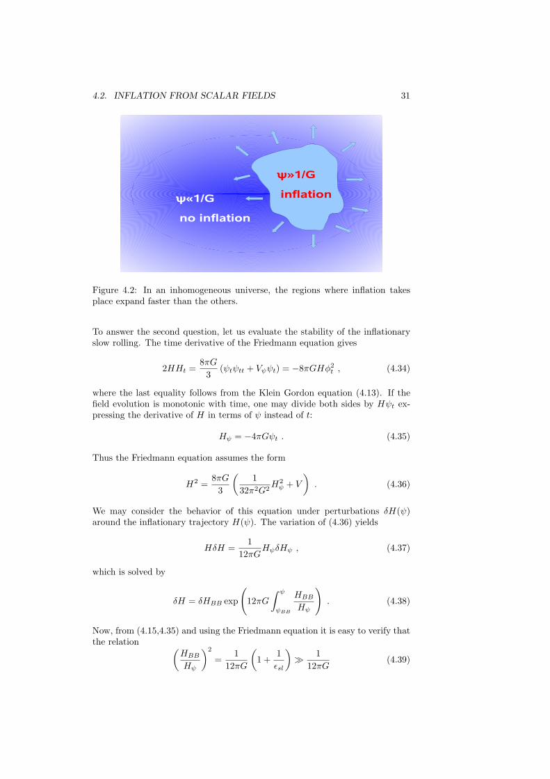
As we have seen, the inflation has the capability of solving the horizon andflatness problems of pre-inflationary cosmology. However, one may ask howlikely is that inflation starts if the universe is inhomogeneous, and how stable isthe process after it started.The first question is answered only qualitatively, through the picture in figure4.2. Simply, the regions in which the conditions are appropriate for inflationto start undergo inflation, expanding faster than the others, by means of theinflationary mechanism itself. The example in the figure refers to the case of thechaotic inflation, in which the conditions for inflation are given just in termsof the field value. Therefore, after some time the inflating regions occupy adominant and increasing fraction of volume, while the portion of space which isnot undergoing inflation vanishes eventually. In this sense, the onset of inflationis a favourite process in inhomogeneous universe.

4.2. INFLATION FROM SCALAR FIELDS 31

Figure 4.2: In an inhomogeneous universe, the regions where inflation takesplace expand faster than the others.

To answer the second question, let us evaluate the stability of the inflationaryslow rolling. The time derivative of the Friedmann equation gives

2HHt =8πG

3(ψtψtt + Vψψt) = −8πGHφ2

t , (4.34)

where the last equality follows from the Klein Gordon equation (4.13). If thefield evolution is monotonic with time, one may divide both sides by Hψt ex-pressing the derivative of H in terms of ψ instead of t:

Hψ = −4πGψt . (4.35)

Thus the Friedmann equation assumes the form

H2 =8πG

3

(1

32π2G2H2ψ + V

). (4.36)

We may consider the behavior of this equation under perturbations δH(ψ)around the inflationary trajectory H(ψ). The variation of (4.36) yields

HδH =1

12πGHψδHψ , (4.37)

which is solved by

δH = δHBB exp

(12πG

∫ ψ

ψBB

HBB

Hψ

). (4.38)

Now, from (4.15,4.35) and using the Friedmann equation it is easy to verify thatthe relation (

HBB

Hψ

)2

=1

12πG

(1 +

1εsl

)À 1

12πG(4.39)

32 CHAPTER 4. INFLATIONARY COSMOLOGY

Figure 4.3: After inflation, the inflaton field rapidly oscillates around the mini-mum of the potential.

holds by virtue of the inflationary expansion. This means that

12πG∫ ψ

ψBB

HBB

Hψ¿√

12πG∫ ψ

ψBB

dψ =√

12πG(ψ − ψBB) (4.40)

if Hψ > 0, while if Hψ < 0 a minus is in front of the last quantity. Usingagain (4.35) one may see that the last quantity in the relation above is alwaysnegative, meaning that δH is exponentially damped along the trajectory, andproving the stability of the inflationary trajectory.

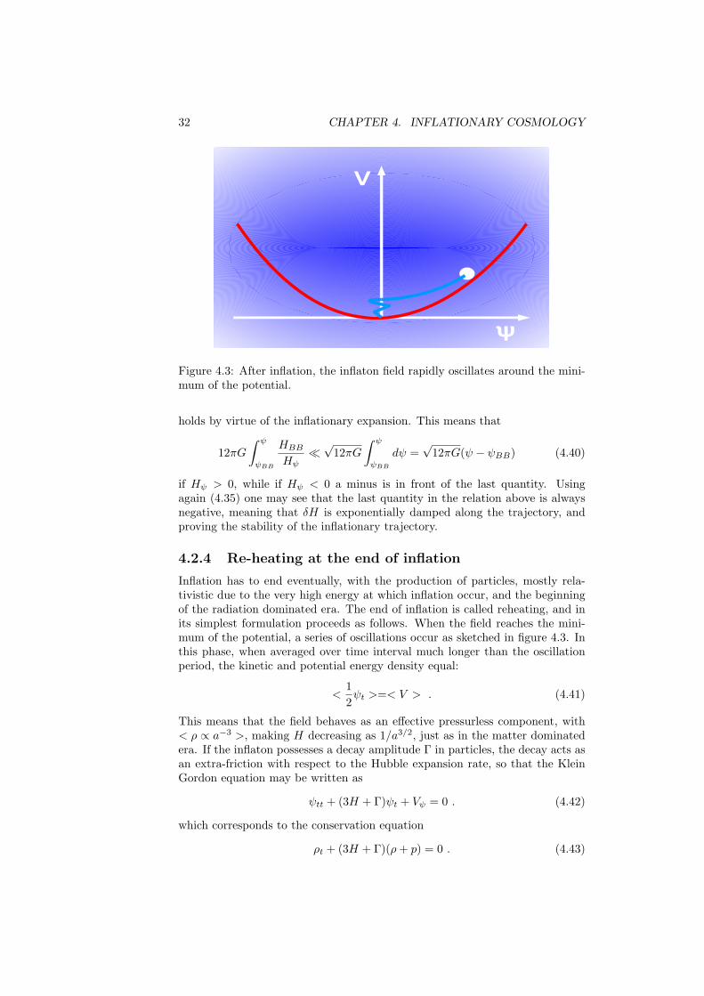
4.2.4 Re-heating at the end of inflation

Inflation has to end eventually, with the production of particles, mostly rela-tivistic due to the very high energy at which inflation occur, and the beginningof the radiation dominated era. The end of inflation is called reheating, and inits simplest formulation proceeds as follows. When the field reaches the mini-mum of the potential, a series of oscillations occur as sketched in figure 4.3. Inthis phase, when averaged over time interval much longer than the oscillationperiod, the kinetic and potential energy density equal:

<12ψt >=< V > . (4.41)

This means that the field behaves as an effective pressurless component, with< ρ ∝ a−3 >, making H decreasing as 1/a3/2, just as in the matter dominatedera. If the inflaton possesses a decay amplitude Γ in particles, the decay acts asan extra-friction with respect to the Hubble expansion rate, so that the KleinGordon equation may be written as

ψtt + (3H + Γ)ψt + Vψ = 0 . (4.42)

which corresponds to the conservation equation

ρt + (3H + Γ)(ρ+ p) = 0 . (4.43)

4.2. INFLATION FROM SCALAR FIELDS 33

We may guess that in order to have inflation, the decay must be negligible withrespect to the amplitude of H during inflation itself. But in the oscillatory phaseof the field which follows the inflationary expansion, H decreases fast, becomingeventually comparable with the decay amplitude of the field. At this point, thedecay takes over, and the energy density stored in the field is transferred in thedecay products.

34 CHAPTER 4. INFLATIONARY COSMOLOGY

Chapter 5

Inflationary perturbations

In this chapter we make a quick review of how cosmological perturbations arethought to be born during inflation. We need ro review the basics of quan-tum field theory in curved spacetimes, before applying them to the inflationaryprocess.

5.1 Quantum fields in curved spacetime

Assume a Minkowski background, and consider the evolution of scalar field ψ,self-interacting only through its mass m. Suppose that the field is also nothomogeneous in space, ψ(t, ~x). The Klein Gordon equation is simply

ψtt −52ψ +m2ψ = 0 , (5.1)

where 52 = ~5 · ~5 is the Laplace operator. It is suitably solved in the Fourierspace, decomposing the field as follows:

ψ(t, ~x) =∑

~k

ψ~k(t)ei~k·~x . (5.2)

The choice of plane waves as expansion function is convenient as they are eigen-gunctions of the at eigenvalue k2 = ~k · ~k of the Laplace operator in the Fourierspace. Thus, still in the Fourier space, the solution to the Klein Gordon equationis analytical:

ψ~ktt + E2~kψ~k = 0 , E~k =

√k2 +m2 , ψ~k(t) ∝ e±iE~k

t . (5.3)

The general solution for (5.1) is therefore

ψ(t, ~x) =∑

~k

12E~k

[a~ke

i(~k·~x−E~kt) + a+

~ke−i(~k·~x−E~k

t)

], (5.4)

where the 2/√

2E~k factor is purely conventional and a~k, a+~k

represent the am-plitude of the field at each mode.The quantization of the system proceeds as usual elevating the field ψ to the role

35

36 CHAPTER 5. INFLATIONARY PERTURBATIONS

of quantum operator on the space of its possible states. , obeying the followingcommutation relations:

[ψ(~x, t), ψ(~x′, t)] = 0 ,[ψ(~x, t), ψ(~x′, t)] = ihδ(~x− ~x′) , (5.5)

[ψt(~x, t), ψt(~x′, t)] = 0 .

We must identify what are numbers and what are operators in the expression(5.4). The only possible choice is represented by a~k and a+

~k; the commutation

relations (5.5) impose the corresponding ones on them:[a~k, a~k′

]= 0 ,[

a~k, a+~k′

]= ihδ(~k − ~k′) , (5.6)

[a+~k, a+~k′

]= 0 .

The space in which these operators act is called the Fock space; it has an emptystate, |0 >, defined by

a~k|0 >= 0∀~k , (5.7)

while a quantum of field at wavenumber is given by

|1~k >= a+~k|0 >= 0∀~k . (5.8)

The field status with many quanta at different wavevectors is given by

|1~k, 1~k, 1~k, ... >= a+~ka+~ka+~k...|0 > , (5.9)

while if ~k is repeated it is easy to see that the commutation relations (5.6) imply

a+~k|n~k > =

√n+ 1|(n+ 1)~k > , (5.10)

a~k|n~k > =√n|(n− 1)~k > . (5.11)

(5.12)

Chapter 6

Testing inflation

37

38 CHAPTER 6. TESTING INFLATION

Chapter 7

Cosmic acceleration today:the dark energy

39