Carmichael numbers and pseudoprimes

Notes by G.J.O. Jameson

Introduction

Recall that Fermat’s “little theorem” says that if p is prime and a is not a multiple of

p, then ap−1 ≡ 1 mod p.

This theorem gives a possible way to detect primes, or more exactly, non-primes: if for

a certain a coprime to n, an−1 is not congruent to 1 mod n, then, by the theorem, n is not

prime. A lot of composite numbers can indeed be detected by this test, but there are some

that evade it. We give ourselves some notation and terminology to discuss them.

For a fixed a > 1, we write F (a) for the set of positive integers n satisfying an−1 ≡ 1

mod n. By Fermat’s theorem, F (a) includes all primes that are not divisors of a.

If n ∈ F (a), then gcd(a, n) = 1, since, clearly, gcd(an−1, n) = 1. Also, an ≡ a mod n;

the reverse implication is true provided that a and n are coprime.

A composite number n belonging to F (a) is called an a-pseudoprime, or a pseudoprime

to the base a. (Some writers require that n should also be odd, but we will not adopt this

convention here.) 2-pseudoprimes are sometimes just called “pseudoprimes”.

A number n that is a-pseudoprime for all a coprime to n is called a Carmichael number,

in honour of R.D. Carmichael, who demonstrated their existence in 1912.

1. Carmichael numbers (1)

1.1. Every Carmichael number is odd.

Proof. If n (≥ 4) is even, then (n− 1)n−1 ≡ (−1)n−1 = −1 mod n, so is not congruent

to 1 mod n. �

We now establish a pleasantly simple description of Carmichael numbers, due to Ko-

rselt. First, we need the following notion. Let a and p be coprime (usually, p will be prime,

but this is not essential). The order of a modulo p, denoted by ordp(a), is the smallest

positive integer m such that am ≡ 1 mod p. Recall [NT4.5]: If ordp(a) = m and r is any

integer such that ar ≡ 1 mod p, then r is a multiple of m. In particular, if p is prime, then

ordp(a) divides into p− 1.

For one half of the following proof (which the reader is at liberty to defer), we need

1

the following theorem (see, e.g. [JJ, chap. 6]):

If p is prime, then there exist a, b such that ordp(a) = p− 1 and ordp2(b) = p(p− 1).

These numbers a, b are called “primitive roots” mod p and p2 respectively. The theorem

equates to the statement that the groups Gp and Gp2 are cyclic.

1.2 THEOREM. A number n is a Carmichael number if and only if n = p1p2 . . . pk, a

product of (at least two) distinct primes, and pj − 1 divides n− 1 for each j.

Proof. Let n be as stated, and let gcd(a, n) = 1. By Fermat’s theorem, for each j, we

have apj−1 ≡ 1 mod pj. Since pj − 1 divides n− 1, an−1 ≡ 1 mod pj. This holds for each

j, hence (by [NT1.15]) an−1 ≡ 1 mod n.

Now assume that n is a Carmichael number. Let p be a prime divisor of n: say n = pku

for some k, where u is not a multiple of p. Take a with ordp(a) = p − 1. By the Chinese

remainder theorem, there exists a1 such that a1 ≡ a mod p and a1 ≡ 1 mod u. Then a1 is

coprime to both p and u, and therefore to n. By hypothesis, an−11 ≡ 1 mod n, so an−1

1 ≡ 1

mod p. Also, ordp(a1) = p− 1. So p− 1 divides n− 1.

Suppose that p2 divides n. Take b with the property stated above, and derive b1 from

it in the same way as a1. Then ordp2(b1) = p(p − 1) and bn−11 ≡ 1 mod p2, so n − 1 is a

multiple of p(p− 1) (so of p). But this is not true, since n is a multiple of p. (An alternative

proof of this part, avoiding the use of b, will be given later.) �

Note 1. The reasoning in the first part of the proof also shows that aλ(n) ≡ 1 mod n,

where λ(n) is the lowest common multiple of p1− 1, . . . , pk − 1. Of course, λ(n) can be very

much smaller than n− 1.

Note 2. If n = p1p2 . . . pk, then pn1 ≡ p1 mod pj for each j (trivial for j = 1, by

Fermat’s theorem for j 6= 1. By [NT1.15], pn1 ≡ p1 mod n. Similarly for each pj. So if n is a

Carmichael number, then pn ≡ p mod n for all primes p, and hence an ≡ a mod n for all a.

At this point, some texts simply state that 561 (= 3×11×17) is a Carmichael number,

and invite the reader to verify it. This is indeed easily done using 1.2. However, this gives

no idea how it, and other examples, can be found, or how to determine whether it is the first

Carmichael number. More generally, how might one detect all the Carmichael numbers up

to a given magnitude N? We will show how to do this, taking N = 3000 (this value is just

large enough to illustrate the principles involved). We start with some easy consequences of

1.2.

2

1.3 LEMMA. Let n = pu. Then p− 1 divides n− 1 if and only if it divides u− 1.

Proof. (n− 1)− (u− 1) = n− u = pu− u = (p− 1)u. The statement follows. �

1.4. A Carmichael number has at least three prime factors.

Proof. Suppose that n has two prime factors: n = pq, where p, q are prime and p > q.

Then p− 1 > q− 1, so p− 1 does not divide q− 1. By 1.3, p− 1 does not divide n− 1. So

n is not a Carmichael number. �

1.5. Suppose that n is a Carmichael number and that p and q are prime factors of n.

Then q is not congruent to 1 mod p.

Proof. Suppose that q ≡ 1 mod p, so that p divides q − 1. Since q − 1 divides n− 1, it

follows that p divides n− 1. But this is not true, since p divides n. �

First, consider numbers with three prime factors: n = pqr, with p < q < r. By 1.2 and

1.3, we require that

(1) p− 1 divides qr− 1, (2) q− 1 divides pr− 1, (3) r− 1 divides pq− 1.

Note that r − 1 6= pq − 1, since r (being prime) is not equal to pq.

With p, q chosen, it is easy to detect the primes r > q such that pqr is a Carmichael

number. Consider the even divisors (if there are any) d of pq − 1 with q < d < pq − 1 and

check whether d + 1 (= r) is prime. Then we have ensured (3), and we check whether (1)

and (2) hold.

We now apply this procedure to find all the Carmichael numbers pqr less than 3000.

We must consider all pairs of primes (p, q) for which pqr < 3000 for at least some primes

r > q. However, because of 1.5, we leave out any combination that has q ≡ 1 mod p (for

example, (3, 7), (3, 13), (5, 11)).

The results are best presented in tabular form, as follows. In each case, we only list

3

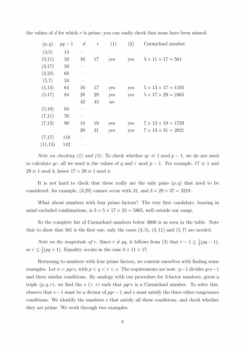
the values of d for which r is prime; you can easily check that none have been missed.

(p, q) pq − 1 d r (1) (2) Carmichael number

(3,5) 14 –

(3,11) 32 16 17 yes yes 3× 11× 17 = 561

(3,17) 50 –

(3,23) 68 –

(5,7) 34 –

(5,13) 64 16 17 yes yes 5× 13× 17 = 1105

(5,17) 84 28 29 yes yes 5× 17× 29 = 2465

42 43 no

(5,19) 94 –

(7,11) 76 –

(7,13) 90 18 19 yes yes 7× 13× 19 = 1729

30 31 yes yes 7× 13× 31 = 2821

(7,17) 118 –

(11,13) 142 –

Note on checking (1) and (2): To check whether qr ≡ 1 mod p − 1, we do not need

to calculate qr; all we need is the values of q and r mod p − 1. For example, 17 ≡ 1 and

29 ≡ 1 mod 4, hence 17× 29 ≡ 1 mod 4.

It is not hard to check that these really are the only pairs (p, q) that need to be

considered: for example, (3,29) cannot occur with 31, and 3× 29× 37 = 3219.

What about numbers with four prime factors? The very first candidate, bearing in

mind excluded combinations, is 3× 5× 17× 23 = 5865, well outside our range.

So the complete list of Carmichael numbers below 3000 is as seen in the table. Note

that to show that 561 is the first one, only the cases (3, 5), (3, 11) and (5, 7) are needed.

Note on the magnitude of r. Since r 6= pq, it follows from (3) that r − 1 ≤ 12(pq − 1),

so r ≤ 12(pq + 1). Equality occurs in the case 3× 11× 17.

Returning to numbers with four prime factors, we content ourselves with finding some

examples. Let n = pqrs, with p < q < r < s. The requirements are now: p−1 divides qrs−1

and three similar conditions. By analogy with our procedure for 3-factor numbers, given a

triple (p, q, r), we find the s (> r) such that pqrs is a Carmichael number. To solve this,

observe that s−1 must be a divisor of pqr−1 and s must satisfy the three other congruence

conditions. We identify the numbers s that satisfy all these conditions, and check whether

they are prime. We work through two examples.

4

Example 1.1. (p, q, r) = (7, 11, 13). Then pqr = 1001, so s − 1 must be a divisor of

1000. The congruence condition for 6 will be implied by the one for 12, so we can leave it

out. The other two are:

7× 13× s ≡ 1 mod 10; since 7× 13 = 91 ≡ 1 mod 10, this is equivalent to s ≡ 1 mod 10;

7× 11× s ≡ 1 mod 12; since 77 ≡ 5 mod 12, this is equivalent to 5s ≡ 1 mod 12, hence

to s ≡ 5 mod 12.

This pair of conditions is equivalent to s ≡ 41 mod 60 (found by considering 5, 17, 29, 41

until we find a number congruent to 1 mod 10). So s − 1 is congruent to 40 mod 60 and a

divisor of 1000. The only numbers satisfying this are 40 and 100. Since 41 and 101 are prime,

these two values of s are the solution to our problem. (In fact, 7× 11× 13× 41 = 41, 041 is

the smallest 4-factor Carmichael number.)

If pqr is itself a Carmichael number, then the congruence conditions equate to s being

congruent to 1 mod p− 1, q − 1 and r − 1, since (for example) qr ≡ 1 mod p− 1.

Example 1.2. (p, q, r) = (7, 13, 19). By the previous remark, s is congruent to 1 mod 6,

12 and 18, hence congruent to 1 mod 36. Also, s− 1 must divide pqr− 1 = 1728 = 48× 36.

So the possible values for s are of the form 36k + 1, where k is a divisor of 48. We list these

values, indicating by * those that are prime, thereby giving a Carmichael number:

37∗, 73∗, 109∗, 145, 217, 289, 433∗, 577∗, 865.

2. Pseudoprimes

We start by showing how one can find some examples of pseudoprimes. First, a trivial

observation: any composite divisor of a − 1 is a-pseudoprime, since a ≡ 1 mod n. (In yet

another variation of the definition, some writers require that n > a, thereby excluding these

cases). However, by considering divisors of am − 1 instead of a − 1, we obtain an instant

method for generating non-trivial pseudoprimes:

2.1. Suppose, for some m, that n divides am − 1 and n ≡ 1 mod m. Then n ∈ F (a).

Proof. Then am ≡ 1 mod n, and n− 1 is a multiple of m. Hence an−1 ≡ 1 mod n. �

So we factorise am − 1 (for a chosen m) and look for any composite divisors that are

congruent to 1 mod m. In particular, if p and q are prime factors of am− 1, both congruent

to 1 mod m, then pq is such a divisor. Also, if p2 appears in the factorisation, where p ≡ 1

mod m, then p2 is a divisor of the type wanted.

5

Note that when n is even (say m = 2k), the first step in the factorisation is a2k − 1 =

(ak + 1)(ak − 1).

We give two examples for a = 2 and two with a = 3.

Example 2.1. We have 210 − 1 = (25 + 1)(25 − 1) = 33 × 31 = 3 × 11 × 31. Both 11

and 31 are congruent to 1 mod 10, so 11× 31 = 341 is 2-pseudoprime.

Example 2.2. We have 211 − 1 = 2047 = 23× 89. Both 23 and 89 are congruent to 1

mod 11, so 23× 89 is 2-pseudoprime.

Example 2.3. We have 35 − 1 = 242 = 2× 112. Hence 112 = 121 is 3-pseudoprime.

Example 2.4. We have 36 − 1 = 26 × 28 = 23 × 7 × 13. Hence 7 × 13 = 91 is

3-pseudoprime.

You can easily verify that these are the lowest powers of 2 and 3 that generate pseu-

doprimes in this way.

It is also easy to verify that the first two examples are not 3-pseudoprimes, and the

second two are not 2-pseudoprimes (of course, 1.2 and 1.4 show that none of them are

Carmichael numbers).

All these examples are special cases of the following general result, first proved by

Cipolla in 1904.

2.2 PROPOSITION. Let a ≥ 2, and let r be an odd number belonging to F (a), or any

odd prime. Let

n1 =ar − 1

a− 1, n2 =

ar + 1

a + 1.

Then:

(i) if gcd(r, a− 1) = 1, then n1 ∈ F (a) (so is a-pseudoprime if it is composite);

(ii) if gcd(r, a + 1) = 1, then n2 ∈ F (a);

(iii) if gcd(r, a2 − 1) = 1, then n1n2 ∈ PS(a).

Hence there are infinitely many a-pseudoprimes.

Proof. By the geometric series, n1 = 1 + a + · · · + ar−1. This shows that n1 is an

integer, and also that it is odd (obvious if a is even, and a sum of r odd numbers if a is odd).

Similarly for n2. Now n1, n2 and n1n2 divide a2r − 1, so 2.1 will apply in each case if we

can show that n1 and n2 are congruent to 1 mod 2r. Now (a− 1)(n1 − 1) = ar − a. By the

hypothesis (either variant), this is a multiple of r. By Euclid’s lemma, since gcd(r, a−1) = 1,

6

r divides n1−1. Since n1−1 is also even, it is a multiple of 2r, so n1 ≡ 1 mod 2r, as required.

Similarly for n2. �

Example 2.1 is n1n2 for a = 2, r = 5, and Example 2.4 is n1n2 for a = 3, r = 3.

Example 2.2 is n1 for a = 2, r = 11. Example 2.3 is n1 for a = 3, r = 5.

2.3 COROLLARY. If r ∈ F (2), then 2r − 1 ∈ F (2). In particular, any “Mersenne

number” 2p − 1 (p prime) is 2-pseudoprime if it is composite. Further, if r ∈ PS(2), then

2r − 1 ∈ PS(2).

Proof. The only point not included in 2.2 is that if r is composite, then so is 2r − 1 (if

r = st, then 2r = cs, where c = 2t, and cs − 1 = (c− 1)(1 + c + · · ·+ cs−1)). �

We will now work towards a characterisation of pseudoprimes, which of course will have

to incorporate ways of detecting numbers that are not pseudoprimes. We shall illustrate the

results by finding all the 2-pseudoprimes less than 1000; as we shall see, this exercise is rather

more complex than the corresponding one for Carmichael numbers.

The notion of the order of a number mod p (defined earlier) is basic for these results.

With a fixed, write ordp(a) = m(p).

2.4. If n ∈ PS(a) and p is a prime factor of n, then m(p) divides n − 1. Further, if

r = n/p, then m(p) divides r − 1. The same applies if p is replaced by any q ∈ F (a).

Proof. an−1 ≡ 1 mod n, so an−1 ≡ 1 mod p. Hence m(p) divides n − 1. Also, m(p)

divides p− 1 and

n− 1 = pr − 1 = (p− 1)r + (r − 1),

so m(p) divides r − 1. The same applies if p is replaced by any q ∈ F (a). �

The analogue of 1.4 for pseudoprimes is:

2.5 COROLLARY. Let n be an a-pseudoprime. If p and q are prime and p divides

m(q), then p and q cannot both be prime factors of n.

Proof. Suppose that q is a prime factor of n and p divides m(q). Then m(q) divides

n− 1, so p divides n− 1. Hence p does not divide n. �

We can derive a complete characterisation of square-free pseudoprimes:

2.6 PROPOSITION. Let n = p1p2 . . . pk, where k ≥ 2 and the numbers pj are distinct

primes that do not divide into a. Let rj = n/pj for each j. Then the following three

statements are equivalent:

7

(i) n is a-pseudoprime,

(ii) m(pj) divides n− 1 for each j,

(iii) m(pj) divides rj − 1 (equivalently, arj−1 ≡ 1 mod pj) for each j.

Proof. We have seen in 2.4 that (i) implies (ii) and (iii)

(ii) implies (i): If (ii) holds, then an−1 ≡ 1 mod pj for each j, hence an−1 ≡ 1 mod n.

(iii) implies (ii), since m(pj) divides pj − 1 and n− 1 = (pj − 1)rj + (rj − 1). �

Clearly, (ii) and (iii) correspond to 1.2 and 1.3 for Carmichael numbers,

We will now find all the square-free 2-pseudoprimes less than 1000. Continue to write

m(p) for ordp(2)). It is not hard to determine m(p):

Example 2.5. Find ord31(2). Denote it by m. Note that 25 = 32 ≡ 1 mod 31. So m

divides 5. Since 5 is prime, m = 5.

We now simply record the values of m(p) for primes p up to 31.

p 3 5 7 11 13 17 19 23 29 31

m(p) 2 4 3 10 12 8 18 11 28 5

We start with numbers with two prime factors. Let n = pq, with p < q. For this special

case, the characterisation in 2.6 (with a = 2) reduces to the following, which we state in two

equivalent forms

(i) 2q−1 ≡ 1 mod p and 2p−1 ≡ 1 mod q;

(ii) m(p) divides q − 1 and m(q) divides p− 1.

So, given p, the only candidates for q are divisors of 2p−1−1. The product pq will then

be 2-pseudoprime if m(p) divides q − 1 (we call this the “m(p) test”). For each p ≤ 23, it is

not hard to find the full factorisation of 2p−1 − 1, helped by the fact that p− 1 is even and

the knowledge that p itself must be a factor. This process will detect all the 2-pseudoprimes

of the form pq; some of them may be larger than 1000, but out of generosity we will include

them!

To start with,

22 − 1 = 3, 24 − 1 = 3× 5, 26 − 1 = 32 × 7,

showing that there are no cases with p equal to 3, 5 or 7. For 11 ≤ p ≤ 23, we tabulate the

results as follows:

8

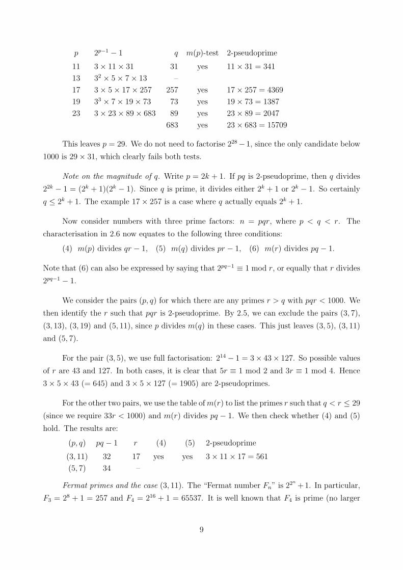
p 2p−1 − 1 q m(p)-test 2-pseudoprime

11 3× 11× 31 31 yes 11× 31 = 341

13 32 × 5× 7× 13 –

17 3× 5× 17× 257 257 yes 17× 257 = 4369

19 33 × 7× 19× 73 73 yes 19× 73 = 1387

23 3× 23× 89× 683 89 yes 23× 89 = 2047

683 yes 23× 683 = 15709

This leaves p = 29. We do not need to factorise 228− 1, since the only candidate below

1000 is 29× 31, which clearly fails both tests.

Note on the magnitude of q. Write p = 2k + 1. If pq is 2-pseudoprime, then q divides

22k − 1 = (2k + 1)(2k − 1). Since q is prime, it divides either 2k + 1 or 2k − 1. So certainly

q ≤ 2k + 1. The example 17× 257 is a case where q actually equals 2k + 1.

Now consider numbers with three prime factors: n = pqr, where p < q < r. The

characterisation in 2.6 now equates to the following three conditions:

(4) m(p) divides qr − 1, (5) m(q) divides pr − 1, (6) m(r) divides pq − 1.

Note that (6) can also be expressed by saying that 2pq−1 ≡ 1 mod r, or equally that r divides

2pq−1 − 1.

We consider the pairs (p, q) for which there are any primes r > q with pqr < 1000. We

then identify the r such that pqr is 2-pseudoprime. By 2.5, we can exclude the pairs (3, 7),

(3, 13), (3, 19) and (5, 11), since p divides m(q) in these cases. This just leaves (3, 5), (3, 11)

and (5, 7).

For the pair (3, 5), we use full factorisation: 214 − 1 = 3× 43× 127. So possible values

of r are 43 and 127. In both cases, it is clear that 5r ≡ 1 mod 2 and 3r ≡ 1 mod 4. Hence

3× 5× 43 (= 645) and 3× 5× 127 (= 1905) are 2-pseudoprimes.

For the other two pairs, we use the table of m(r) to list the primes r such that q < r ≤ 29

(since we require 33r < 1000) and m(r) divides pq − 1. We then check whether (4) and (5)

hold. The results are:

(p, q) pq − 1 r (4) (5) 2-pseudoprime

(3, 11) 32 17 yes yes 3× 11× 17 = 561

(5, 7) 34 –

Fermat primes and the case (3, 11). The “Fermat number Fn” is 22n+1. In particular,

F3 = 28 + 1 = 257 and F4 = 216 + 1 = 65537. It is well known that F4 is prime (no larger

9

Fermat primes are known). Given this fact, we can easily revisit the case (p, q) = (3, 11) and

apply full factorisation: 232 − 1 = 3 × 5 × 17 × 257 × F4. Both 257 and F4 satisfy (4) and

(5), so both give a 2-pseudoprime 3× 11× r.

As in the case of numbers with two prime factors, if pqr is 2-pseudoprime and pq =

2k + 1, then r must divide either 2k + 1 or 2k − 1. The example 3× 11× F4 is a case where

r equals 2k + 1.

What about numbers with four prime factors? Given the exclusions resulting from 2.5,

the first candidate is 3× 5× 17× 23 = 5865, well outside our chosen range. (The first such

2-pseudoprime is actually 5 × 7 × 17 × 19 = 11305.) So we can now give the full list of

square-free 2-pseudoprimes less than 1000:

11× 31 = 341, 3× 11× 17 = 561, 3× 5× 43 = 645.

We saw in Example 2.3 that 112 ∈ PS(3), so pseudoprimes, unlike Carmichael numbers,

are not always square-free. We now extend the previous characterisation to general numbers.

2.7 LEMMA. If b ≡ 1 mod p, then: (i) bp ≡ 1 mod p2, (ii) bpk−1 ≡ 1 mod pk for all

k ≥ 2.

Proof. (i) By the geometric series,

bp − 1 = (b− 1)(1 + b + b2 + · · ·+ bp−1).

By hypothesis, b − 1 is a multiple of p. The second bracket is the sum of p terms, each

congruent to 1 mod p. Hence it is congruent to p mod p, in other words, again a multiple

of p. So bp − 1 is a multiple of p2. (Alternatively, write b = 1 + sp and use the binomial

theorem).

(ii) Induction. Assume the statement for a particular k. Write c = bpk−1. By assump-

tion, pk divides c− 1, and

bpk − 1 = cp − 1 = (c− 1)(1 + c + c2 + · · ·+ cp−1).

As in (i), the second bracket is a multiple of p, hence bpk − 1 is a multiple of pk+1. �

We continue the standing assumption that p is prime and a is not a multiple of p.

2.8 THEOREM. Suppose that n = pkr ∈ PS(a) for some k ≥ 2 and r (we do not

exclude r being a multiple of p). Then: (i) am ≡ 1 mod pk, where m = ordp(a), (ii)

pk ∈ PS(a).

10

Proof. Again we give the proof for k = 2 first, since it is simpler. Since n ∈ PS(a), we

have an ≡ a mod n, hence an ≡ a mod p2. By 2.7, with b = am, we have apm ≡ 1 mod p2.

So

am ≡ amn = ap2rm = (apm)pr ≡ 1 mod p2.

Statement (ii) follows, since m divides p2 − 1.

Now consider k ≥ 3. By 2.7, ampk−1 ≡ 1 mod pk. The result follows as before, since

mn = mpkr = (mpk−1)pr. �

In particular, if pk ∈ PS(a) for some k > 2, then p2 ∈ PS(a).

So to determine whether pk is in PS(a), we only have to consider am instead of apk−1,

a big simplification! Two further consequences are:

2.9 COROLLARY. If (and only if) pk ∈ PS(a), then ap−1 ≡ 1 mod pk.

Proof. p− 1 is a multiple of m. �

2.10 COROLLARY. If pk is in PS(a) and m is even, say m = 2n, then an ≡ −1

mod pk.

Proof. By 2.8, pk divides into a2n − 1 = (an + 1)(an − 1), so appears in the (unique)

prime factorisation of this product. By the definition of m, p does not divide an − 1. Hence

pk is a factor of an + 1. �

Alternative proof that Carmichael numbers are square-free. Suppose that n = pkr is a

Carmichael number, where k ≥ 2 and r is not a multiple of p. Then by CPS11, ap−1 ≡ 1

mod p2 for any a coprime to n. Now by the binomial theorem,

(p + 1)p−1 = 1 + (p− 1)p + tp2

for some integer t; this is congruent to 1− p (so not congruent to 1) mod p2. By the Chinese

remainder theorem, there exists a congruent to p + 1 mod pk and congruent to 1 mod r.

Then a is coprime to pk and to r, hence coprime to n, but ap−1 6≡ 1 mod p2. �

We are now ready to give the fully general characterisation of a-pseudoprimes.

2.11 THEOREM. Suppose that gcd(n, a) = 1 and that n = q1q2 . . . qk, where qj = pkj

j

for distinct primes pj. Let rj = n/qj. Then n is a-pseudoprime if and only if

(i) apj−1 ≡ 1 mod qj for all j

and (ii) arj−1 ≡ 1 mod qj for all j.

11

Proof. Suppose that n is a-pseudoprime. Then 2.8 shows that (i) holds whenever

kj ≥ 2; of course, it holds automatically if kj = 1. Statement (ii) is given by 2.4.

Conversely, if (i) and (ii) hold, then the reasoning in 2.6 applies without change to

show that n ∈ PS(a). �

The two conditions can be combined as follows: let nj = gcd(rj − 1, pj − 1). Then

n ∈ PS(a) iff anj ≡ 1 mod qj for all j. Further, nj = gcd(n − 1, pj − 1), since n − 1 =

(qj − 1)rj + (rj − 1) and pj − 1 divides qj − 1.

By 2.8, (i) is also equivalent to qj ∈ F (a), and to m(pj) = m(qj). Given that this

holds, (ii) is equivalent to m(pj) dividing rj − 1 for each j.

Completion of the search for 2-pseudoprimes below 1000. We can now show quite

quickly that there are no non-square-free 2-pseudoprimes below 1000, so the only 2-pseudoprimes

below 1000 are the three square-free ones already listed, i.e. 341, 561 and 645.

It is enough to show that p2 is not 2-pseudoprime for each prime p ≤ 31. By 2.9, if

p2 ∈ PS(2), then p2 divides 2p−1 − 1. For each p ≤ 23, the full factorisation of 2p−1 − 1 was

given earlier. In each case, we see that p2 is not a factor (although, of course, p is).

It remains to consider 29 and 31. Write just m for m(p). If p2 ∈ PS(2), then 2.8 tells

us that 2m ≡ 1 mod p2; if also m = 2n, then 2.10 says that 2n ≡ −1 mod p2.

p = 29: Then m = 28, so n = 14. Now 27 = 128 = 4× 29 + 12, so (mod 292)

214 ≡ 96× 29 + 144 = 101× 29− 1 ≡ 14× 29− 1 6≡ −1.

p = 31: Then m = 5, and 25 − 1 = 31, not a multiple of 312.

It turns out that the first prime p for which p2 is 2-pseudoprime is 1093 (this was

discovered by Meissner in 1913, long before the age of computers). Long before this, one

might have been tempted to conjecture that there are no such primes! Even more remarkably,

it is now known that there are only two such primes less than 109, namely 1093 and 3511.

Searching for 3-pseudoprimes. The reader may choose to undertake a similar exercise

for 3-pseudoprimes. To assist the process, we provide a table of values of m(p) = ordp(3) for

p ≤ 43:

p 5 7 11 13 17 19 23 29 31 37 41 43

ordp(3) 4 6 5 3 16 18 11 28 30 18 8 42

12

By definition, 3 is no longer permitted as a prime factor, which shortens the list of

pairs (p, q). If we adhere to the form of the definition that allows even numbers, then 2 is

permitted, but by 2.5, it can only be combined with q having m(q) odd.

Since 112 is 3-pseudoprime, it is necessary to investigate numbers of the form 112q (it

turns out that there are no other primes p ≤ 31 with p2 3-pseudoprime). By 2.11, for 112q to

be 3-pseudoprime, we require m(11) (= 5) to divide q− 1 and m(q) to divide 120. From the

table above, we see that these conditions are satisfied by 31 and 41 (they are also satisfied

by 61).

The list of 3-pseudoprimes less than 1000 is;

7× 13 = 91 11× 61 = 671

112 = 121 19× 37 = 703

2× 11× 13 = 286 13× 73 = 949

We include one further result on 2-pseudoprimes with two prime factors. Recall that

the numbers Mk = 2k − 1 are the “Mersenne numbers”. We need two lemmas:

2.12 LEMMA. If gcd(j, k) = 1, then gcd(Mj, Mk) = 1.

Proof. Let gcd(Mj, Mk) = d. Then 2j and 2k are congruent to 1 mod d. So ordd(2)

divides both j and k, hence is 1. This means that 2 ≡ 1 mod d, hence d = 1. �

2.13 LEMMA. If k ≥ 5 is not a multiple of 3, then 2k +1 has prime factors other than

3.

Proof. 23 ≡ −1 mod 9, so 2r ≡ −1 mod 9 only when r is an odd multiple of 3, hence

2k is not congruent to −1 mod 9. So 2k +1 is not of the form 3s, and has prime factors other

than 3. �

2.14 PROPOSITION. There are infinitely many 2-pseudoprimes with two prime fac-

tors.

Proof. Take any prime k ≥ 5. Choose a prime factor p of 2k − 1 and a prime factor

q 6= 3 of 2k + 1. Then 2k ≡ 1 mod p: since k is prime, m(p) = k. So p− 1 is a multiple of

k, and hence (since it is even) of 2k. Similarly, 22k ≡ 1 mod q, so m(q) divides 2k, hence is

either 2 or 2k. But if m(q) = 2, then q divides 22 − 1 = 3, so q = 3, contrary to our choice.

So m(q) = 2k, and q − 1 is a multiple of 2k. By 2.6, pq ∈ PS(2). Finally, if k′ is another

prime, with corresponding p′, q′, then by Lemma 2.12, p is different from p′ and q′ (note that

q′ divides M2k′ and gcd(k, 2k′) = 1), so pq 6= p′q′. �

13

3. The bases for which a given number is pseudoprime

So far, the emphasis has been on finding the members n of PS(a) for a fixed a. Instead,

we will now fix an odd, composite number n and focus attention on the set of numbers a for

which n ∈ PS(a), in other words, such that an−1 ≡ 1 mod n. Recall that this necessarily

implies that gcd(a, n) = 1.

If this is satisfied by a, it is also satisfied by any b congruent to a mod n. So we only

need to consider congruence classes mod n, reducing the problem to a finite one.

We denote by Gn the group of congruence classes (alias residue classes) coprime to n.

This can be described as the group of units in the ring Zn of (all) congruence classes mod

n. We write r (or r when r is a longer expression) for the congruence class containing r.

For a finite set S, we denote by |S| (when there is no danger of confusion) the number

of members of S. By definition, |Gn| = φ(n).

The statement an−1 ≡ 1 mod n is equivalent to an−1 = 1. We denote by Pn the set of

elements of Gn that satisfy this, in other words, the set of a (mod n) for which n ∈ PS(a).

By definition, n is a Carmichael number if and only if Pn = Gn.

Of course, it is of no great interest to say that n ∈ PS(1). However, we must recognise

that 1 is an element (indeed, an important one) of Pn.

3.1. Pn is a subgroup of Gn, hence |Pn| divides φ(n).

Proof. In any abelian group G with identity e, it is elementary that {a ∈ G : am = e}is a subgroup for any positive integer m. Also, the order of a subgroup divides |G|. �

So if n is not a Carmichael number, then |Pn| is a proper divisor of φ(n); in particular,

|Pn| ≤ 12φ(n).

3.2. If a ∈ Pn, then (n− a) ∈ Pn. In particular, −1 ∈ Pn.

Proof. Since n− 1 is even, (−a)n−1 = an−1. �

Recall the characterisation of a-pseudoprimes in 2.11. One way to state it is as follows.

Let n = q1q2 . . . qk, where qj = pkj

j for distinct primes pj, and let rj = n/qj. let nj =

gcd(n− 1, pj − 1) = gcd(rj − 1, pj − 1). Then n ∈ PS(a) iff anj ≡ 1 mod qj for all j.

This can be read equally as a characterisation of the elements of Pn. We deduce an

expression for |Pn|. We use again the fact that the group Gq is cyclic if q = pr for an odd

14

prime p, together with the following lemma.

3.3 LEMMA. Let G be a cyclic group of order n, and let k ≥ 1. Then the number of

elements a ∈ G satisfying ak = e is gcd(k, n).

Proof. Let u be a generator of G, so u has order n. Let gcd(k, n) = d, and write

k = k1d, n = n1d. Then gcd(k1, n1) = 1. Let a = uj. Then ak = ujk = e iff n divides jk,

equivalently n1 divides jk1. By Euclid’s lemma, this occurs iff j is a multiple of n1. So the

distinct elements uj satisfying the condition are given by j = rn1 for 1 ≤ r ≤ d. �

3.4 THEOREM. Let n be as above. Then |Pn| = n1n2 . . . nk.

Proof. Since nj divides φ(qj), there are exactly nj numbers a (mod qj) satisfying

anj ≡ 1 mod qj. By the Chinese remainder theorem, there are n1n2 . . . nk elements (mod n)

that satisfy this condition for all j. �

This theorem can be seen as a generalisation of Korselt’s characterisation of Carmichael

numbers (Theorem 1.2): to have |Pn| = φ(n), we require that φ(n) =∏k

j=1(pj − 1) (so n is

square-free) and nj = pj − 1, so pj − 1 divides n− 1, for each j.

We will now describe the group Pn in some particular cases.

3.5. Let n = pq, where p, q are prime and 2 < p < q. Let gcd(p− 1, q − 1) = g. Then

|Pn| = g2. The set Pn consists of the elements a satisfying ag ≡ 1 mod p and mod q.

Proof. In the notation of 4.4, n1 = n2 = g. However, we already know from 2.6 that

to have a ∈ Pn we require ordp(a) to divide q − 1, and hence to divide g, and similarly for

ordq(a). �

In particular, if p− 1 divides q − 1, then |Pn| = (p− 1)2. The members of Pn are the

numbers satisfying ap−1 ≡ 1 mod q − 1.

We specialise further to numbers of the form n = pq with q − 1 = 2(p − 1). Clearly,

for such numbers we have |Pn| = 12φ(n) (one might call them “semi-Carmichael numbers”).

Note that if p > 3, then for q to be prime, p must be congruent to 1 mod 6, since if p ≡ 5

mod 6, then q ≡ 3 mod 6, so is a multiple of 3. So p = 6k+1 and q = 12k+1 for some k. The

members of Pn are those satisfying ap−1 ≡ 1 mod q; by Euler’s criterion, this is equivalent

to a being a quadratic residue mod q, or (a | q) = 1 in the notation of the Legendre symbol.

We now identify the cases when 2, 3 and 5 belong to Pn, using the following well-known

facts:

15

(2 | q) = 1 iff q ≡ ±1 mod 8,

(3 | q) = 1 iff q ≡ ±1 mod 12,

(5 | q) = 1 iff q ≡ ±1 mod 5.

3.6. Suppose that p (≥ 5) and q = 2p− 1 are prime, and n = pq. Then:

(i) 2 ∈ Pn iff p ≡ 1 mod 4;

(ii) 3 ∈ Pn in all cases

(iii) 5 ∈ Pn iff p ≡ 1 mod 10.

Proof. (i) If p = 4r + 1, then q = 8r + 1, so (2 | q) = 1. If p = 4r + 3, then q = 8r + 5,

so (2 | q) = −1.

(ii) As seen above, q = 12k + 1 for some k.

(iii) Corresponding to the values 1, 2, 3, 4 for p mod 5, the values for q mod 5 are 1,

3, 0, 2. Only the first case (in which case p ≡ 1 mod 10) gives (5 | q) = 1. �

We list the first few pairs (p, q) with both prime. The cases with p ≡ 1 mod 4 (so that

pq ∈ PS(2)) are indicated by ∗.

p 7 19 31 37∗ 79 97∗ 139 157∗

q 13 37 61 73 157 193 277 313

Next, we consider n = p2. By 3.4, |Pn| = p − 1. However, we will establish a direct

description of Pn without relying on the theorem that Gn is cyclic. Note first that for any b

not a multiple of p, we have bp(p−1) ≡ 1 mod p2: this is a case of the Euler-Fermat theorem,

but it also follows from 2.7 applied to bp−1.

3.7 LEMMA. Suppose that b and c are not multiples of p. Then bp ≡ cp mod p2 if and

only if b ≡ c mod p.

Proof. Suppose that b ≡ c mod p. We have

bp − cp = (b− c)(bp−1 + bp−2c + · · ·+ cp−1).

Exactly as in 2.7, it follows that bp − cp is a multiple of p2.

Conversely, if this holds, then b ≡ bp ≡ cp ≡ c mod p. �

3.8. Let n = p2. Then Pn consists of the p − 1 elements (bp) (1 ≤ b ≤ p − 1), which

are distinct in Gn.

16

Proof. If a ∈ Pn, then by 2.7, ap−1 ≡ 1 mod p2, so a ≡ ap mod p2. Conversely, if a ≡ xp

mod p2, then ap−1 ≡ xp(p−1) ≡ 1 mod p2.

Every x ∈ Gn is congruent (mod p) to some b with 1 ≤ b ≤ p − 1. By the Lemma,

xp ≡ bp mod p2, and further, the elements bp are distinct mod p2. �

We can now revisit the observed scarcity of primes p such that p2 ∈ PS(2), or equiva-

lently, such that 2 ∈ Pn (where n = p2). Of the p(p− 1) elements of Gn, just p− 1 belong to

Pn, two of which are 1 and −1. If the others, in some sense, are equally distributed across

the available values, then it would be reasonable to conclude that the “probability” (again

in some sense) of 2 belonging to Pn is (p − 3)/p(p − 1) < 1/p. So the expected number of

primes p < x such that p2 ∈ PS(2) would be∑

p<x1p, which is known to be approximated

by log log x. Now log log 109 ≈ 3.03, so we should not be surprised that there are only two

such primes less than 109.

4. Carmichael numbers (2)

This section is largely devoted to further results on Carmichael numbers with three

prime factors. We have shown how to find the Carmichael numbers of form pqr for a given

(p, q). We now establish a much more striking fact: there are only finitely many Carmichael

numbers of the form pqr for a given p. Furthermore, we can give an upper bound for the

number of them and describe a systematic way of finding them.

We restate the previous (1),(2),(3) more explicitly: n = pqr is a Carmichael number if

and only if there are integers h1, h2, h3 such that

qr − 1 = h1(p− 1), (7)

pr − 1 = h2(q − 1), (8)

pq − 1 = h3(r − 1). (9)

The rough significance of these numbers is shown by the approximations h1 ≈ qr/p (etc.)

when p, q, r are large.

4.1. We have 2 ≤ h3 ≤ p− 1.

Proof. Since r − 1 > q, we have qh3 < pq, hence h3 < p. Since both are integers,

h3 ≤ p− 1. Also, h3 6= 1 since r 6= pq (r is prime!). So h3 ≥ 2. �

The essential point is that we can express q and r in terms of p, h2 and h3:

17

4.2. We have

q − 1 =(p− 1)(p + h3)

h2h3 − p2. (10)

Proof. By (8) and (9),

h2(q − 1) = p(r − 1) + (p− 1)

=p

h3

(pq − 1) + (p− 1),

so

h2h3(q − 1) = p(pq − 1) + h3(p− 1) = p[p(q − 1) + (p− 1)] + h3(p− 1),

hence

(h2h3 − p2)(q − 1) = (p + h3)(p− 1). �

Once p, q and h3 are known, r is determined by (9).

4.3 THEOREM. Let p be prime. Then there are only finitely many 3-factor Carmichael

numbers with smallest prime factor p. Denote this number by f3(p). Then

f3(p) ≤ (p− 2)(log p + 2).

Moreover, for any ε > 0, we have f3(p) < εp log p for sufficiently large p, so in fact

f3(p)

p log p→ 0 as p →∞.

Proof. Choose h3 satisfying 2 ≤ h3 ≤ p− 1. Write h2h3 − p2 = ∆. We will work with

∆ rather than h2. When ∆ is chosen, q is determined by (10) and then r by (9). By (10),

∆ =(p− 1)(p + h3)

q − 1.

Clearly, ∆ is a positive integer, so ∆ ≥ 1. Also, since p − 1 < q − 1, we have ∆ < p + h3,

so in fact ∆ ≤ p + h3 − 1, and ∆ must lie in an interval of length p + h3 − 2. In addition,

∆ must be congruent to −p2 mod h3, so each block of length h3 contains only one possible

value for ∆. Hence the number of choices for ∆ is no more than

p + h3 − 2

h3

+ 1 =p− 2

h3

+ 2.

We now add over the possible values of h3 and use the well-known fact that∑p

h=21h

< log p

to obtain

f3(p) ≤p−1∑h=2

(p− 2

h+ 2

)< (p− 2)(log p + 2).

18

You at liberty not to bother with the second half of the proof! For those bothering, the

point is that the estimation just found took no notice of the fact that ∆ also has to be a divisor

of (p− 1)(p + h3). We use the well-known fact that for any ε > 0, τ(n)/nε → 0 as n →∞,

where τ(n) is the number of divisors of n. So the number of choices for ∆ is also bounded by

τ [(p−1)(p+h3)], which is less than pε for large enough p (since (p−1)(p+h3) < 2p2). Using

this bound for h3 ≤ p1−ε and the previous one for h3 > p1−ε, together with the elementary

estimation∑

y<n≤x1n≤ log x− log y+1, we see that f3(p) ≤ S1 +S2, where S1 = p1−εpε = p

and

S2 ≤∑

p1−ε<h<p

(p

h+ 2

)≤ p(ε log p + 1) + 2p = εp log p + 3p,

so f3(p) < εp log p + 4p < 2εp log p for large enough p. Of course, we can now replace 2ε

by ε. �

Note. Using known bounds for the divisor function, the estimate can be refined to

f3(p) ≤ (p log p)/(log log p) for large enough p (see [Jam]).

The proof of 4.3 also amounts to a procedure for finding the Carmichael numbers pqr

for a given p. We choose h3, then search for possible values of ∆. They have to satisfy:

∆ ≤ p + h3 − 1,

∆ ≡ −p2 mod h3,

∆ divides (p− 1)(p + h3).

For example, if h3 = 2, the second condition restricts ∆ to odd values.

We list the values of ∆ satisfying these conditions. For each of them, q is defined

by q − 1 = (p− 1)(p + h3)/∆. Of course, q may or may not be prime. If it is, we continue,

deriving r from (9). (The r defined this way will always be an integer: by the expression

for h2(q − 1) in the proof of 4.2, h3 divides p(pq − 1); now by Euclid’s lemma, h3 divides

pq−1). The algebra of 4.2, taken in reverse, shows that we have ensured that (8) is satisfied.

We still have to check whether r is prime and whether qr ≡ 1 mod (p − 1): if both these

things happen, then pqr is a Carmichael number. Furthermore, this process will detect all

Carmichael numbers of the form pqr.

We now work through the cases p = 3, 5, 7. We present the numbers in factorised form

without multiplying them out First, take p = 3. The only value for h3 is 2. We require ∆ to

be odd, no greater than 4, and a divisor of 10. The only choice is ∆ = 1, giving q = 11. By

(9), 2(r− 1) = 32, so r = 17. Clearly, qr ≡ 1 mod 2. So 3× 11× 17 is a Carmichael number,

and it is the only one with p = 3.

19

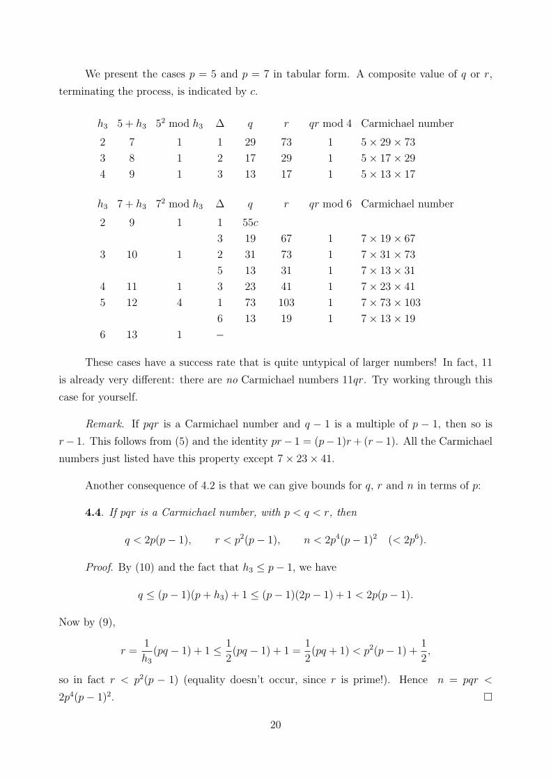
We present the cases p = 5 and p = 7 in tabular form. A composite value of q or r,

terminating the process, is indicated by c.

h3 5 + h3 52 mod h3 ∆ q r qr mod 4 Carmichael number

2 7 1 1 29 73 1 5× 29× 73

3 8 1 2 17 29 1 5× 17× 29

4 9 1 3 13 17 1 5× 13× 17

h3 7 + h3 72 mod h3 ∆ q r qr mod 6 Carmichael number

2 9 1 1 55c

3 19 67 1 7× 19× 67

3 10 1 2 31 73 1 7× 31× 73

5 13 31 1 7× 13× 31

4 11 1 3 23 41 1 7× 23× 41

5 12 4 1 73 103 1 7× 73× 103

6 13 19 1 7× 13× 19

6 13 1 −

These cases have a success rate that is quite untypical of larger numbers! In fact, 11

is already very different: there are no Carmichael numbers 11qr. Try working through this

case for yourself.

Remark. If pqr is a Carmichael number and q − 1 is a multiple of p − 1, then so is

r− 1. This follows from (5) and the identity pr− 1 = (p− 1)r + (r− 1). All the Carmichael

numbers just listed have this property except 7× 23× 41.

Another consequence of 4.2 is that we can give bounds for q, r and n in terms of p:

4.4. If pqr is a Carmichael number, with p < q < r, then

q < 2p(p− 1), r < p2(p− 1), n < 2p4(p− 1)2 (< 2p6).

Proof. By (10) and the fact that h3 ≤ p− 1, we have

q ≤ (p− 1)(p + h3) + 1 ≤ (p− 1)(2p− 1) + 1 < 2p(p− 1).

Now by (9),

r =1

h3

(pq − 1) + 1 ≤ 1

2(pq − 1) + 1 =

1

2(pq + 1) < p2(p− 1) +

1

2,

so in fact r < p2(p − 1) (equality doesn’t occur, since r is prime!). Hence n = pqr <

2p4(p− 1)2. �

20

Similar results apply to numbers with four prime factors, n = pqrs with p < q < r < s

and (p, q) given. All we have to do is substitute pq for p in our previous reasoning. It doesn’t

make any difference that pq is not prime until the final step, where of course the congruences

for p− 1 and q − 1 must be checked separately. We define h4 by h4(s− 1) = pqr − 1, from

which it follows that 2 ≤ h4 ≤ pq − 1 (and also h4 cannot be a multiple of p or q). Identity

(10) becomes r − 1 = (pq − 1)(pq + h4)/∆, where ∆ = h3h4 − p2q2, so that

∆ =(pq − 1)(pq + h4)

r − 1< p(pq + h4).

Of course, ∆ also has to divide (pq−1)(pq+h4). This limits the number of possible values for

it to (pq)ε (for any given ε > 0) for large enough pq, so the number of Carmichael numbers

of this form is bounded by (pq)1+ε.

Returning to Carmichael numbers with three prime factors, let C3(x) be the number of

such numbers not greater than x. We can give an estimation of C3(x) using Theorem 4.3 and

Chebyshev’s well-known estimate for prime numbers, which states the following: let P (x)

denote the set of primes not greater than x, and let θ(x) =∑

p∈P (x) log p. Then θ(x) ≤ cx

for all x, where c is a constant not greater than log 4.

4.5. There is a constant C ≤ 2 log 4 such that C3(x) ≤ Cx2/3 for all x > 2.

Proof. Use 4.3 in the form f3(p) ≤ 2p log p. If n = pqr ≤ x, then p < x1/3. Hence

C3(x) ≤∑

p∈P (x1/3)

2p log p ≤ 2x1/3θ(x1/3) ≤ 2cx2/3. �

For a Carmichael number n = pqr, let g be the gcd of p−1, q−1 and r−1. Obviously,

g is even and g ≤ p− 1. Write

p− 1 = ag, q − 1 = bg, r − 1 = cg, (11)

so that a < b < c (hence b ≥ 2, c ≥ 3 and abc ≥ 6). Clearly, abcg3 < n, so g < n1/3.

4.6. We have g = gcd(p− 1, q − 1) (etc.), hence a, b, c are pairwise coprime.

Proof. Let gcd(p− 1, q − 1) = g0. Now qr − 1 is a multiple of (p− 1), so of g0. But g0

divides q − 1, and qr − 1 = (q − 1)r + (r − 1). So g0 divides r − 1, hence g0 = g. �

Hence a = 1 iff q− 1 is a multiple of p− 1. As remarked earlier, this occurs frequently.

Example. For n = 7× 13× 19, we have g = 6, a = 1, b = 2, c = 3.

There are numerous identities and inequalities linking these numbers. First, (7), (8)

and (9) can be restated as follows.

21

4.7. We have

h1a = bcg + b + c, h2b = acg + a + c, h3c = abg + a + b. (12)

Proof. (7) says h1ag = (bg + 1)(cg + 1)− 1 = bcg2 + bg + cg. Similarly for (8), (9). �

Note that h3c can also be written as aq + b and as bp + a.

4.8. Let

E = (bc + ca + ab)g + a + b + c.

Then there is an integer k such that E = kabc.

Proof. By 4.7, we have

E = a(b + c)g + a + (bcg + b + c) = a(b + c)g + a + h1a,

so a divides E. Similarly for b and c. Since a, b, c are pairwise coprime, abc divides E. �

4.9. If a, b, c are given, then there is only one possible choice for g mod abc.

Proof. Write bc + ca + ab = S. If d divides S and a, then it divides bc and a, so

d = 1. So gcd(S, a) = 1. Similarly for b, c, hence gcd(S, abc) = 1. By 4.8, g has to satisfy

Sg ≡ −a− b− c mod abc. This determines g uniquely mod abc. �

Conversely, suppose that a, b, c (pairwise coprime) are given, and that g satisfies Sg ≡−a − b − c mod abc, so that E is a multiple of abc. Let p, q, r be defined by (11) and let

n = pqr. Then the algebra in 4.7 and 4.8, in reverse, shows that (12) holds for certain

integers h1, h2, h3, and hence that (7), (8), (9) hold. So if p, q, r are prime, then n is

a Carmichael number. This gives a procedure for searching for Carmichael numbers with

specified a, b, c.

Example. (a, b, c) = (1, 2, 3). The condition for g is 11g ≡ −6 mod 6, hence g = 0 mod

6. The first three cases that give three primes are:

g = 6: 7× 13× 19; g = 36: 37× 73× 109; g = 210: 211× 421× 631.

In general, g = 6m, giving p = 6m + 1, q = 12m + 1, r = 18m + 1. If it could be shown

that there are infinitely many values of m such that these three are all prime, then it would

follow that there are infinitely many Carmichael numbers with three prime factors. However,

this is a typical example of a whole family of problems about prime numbers that remain

unsolved. We remark that to avoid any of p, q, r being a multiple of 5, we need m to be

congruent to 0 or 1 mod 5.

22

Example. (a, b, c) = (2, 3, 5). Then 31g ≡ −10 ≡ 20 mod 30, so g ≡ 20 mod 30. The

first three cases are:

g = 20: 41× 61× 101; g = 50: 101× 151× 251; g = 140: 281× 421× 701.

In general, g = 30m + 20, giving p = 60m + 41, q = 90m + 61, r = 150m + 101.

We mention some inequalities for these quantities.

4.10 We have a ≤ 3g − 1 and a <√

3n1/6.

Proof. Recall that a < b < c and g ≥ 2. By 4.8,

kab = g

(a + b +

ab

c

)+

(1 +

a

c+

b

c

)< g(2a + b) + 3 ≤ g(3b− 2) + 3 < 3bg,

so ka < 3g, hence a ≤ ka ≤ 3g − 1. Hence also a2 < 3ag < 3p ≤ 3n1/3. �

4.11. We have p < 3g2, q < 18g4, r < 27g6, n < 2.36 g12.

Proof. Since g ≥ 2, we have p = ag + 1 ≤ (3g− 1)g + 1 < 3g2. The other bounds now

follow from 4.4. �

With more care, these estimations can be improved considerably. By 4.11, there are

only finitely many 3-factor Carmichael numbers with a given value of g. In fact, it can be

shown that this number is bounded by an estimate of the form Cεg1+ε. Also, by further

development of this analysis, the estimation of C3(x) in 4.5 has been greatly strengthened

in successive steps. The best current estimate [HBr] is C3(x) ≤ x7/20+ε for large enough x.

A gentle exposition of these results can be seen in [Jam].

5. Concluding remarks

Up to 106, there are just 43 Carmichael numbers and 245 2-pseudoprimes, whereas

there are 78,498 primes – so the original idea of using the Fermat property to detect primes

is not so bad after all!

R.G.E. Pinch [Pi] has computed the Carmichael numbers up to 1018 and the 2-pseudoprimes

up to 1013. Some of his results are as follows. Here, C(x) denotes the number of Carmichael

numbers up to x, C3(x) the number with three prime factors, and P2(x) the number of

23

2-pseudoprimes.x 106 109 1012

C(x) 43 646 8, 241

C3(x) 23 172 1, 000

P2(x) 245 5, 597 101, 629

It was an unsolved problem for many years whether there are infinitely many Carmichael

numbers. The question was resolved in 1994 in a classic article by Alford, Granville and

Pomerance in 1994 [AGP]. Here it was shown, using sophisticated methods, not only that

the answer is yes, but that in fact C(x) > x2/7 for sufficiently large x. The 27

has been

improved to 0.33 by Harman [Har]. (Recall from 2.2 that the corresponding question for

pseudoprimes is very easily answered.)

Pinch’s figures suggest an upper bound of the form xα (with α possibly close to 13) for

C(x), but no such bound is known, and it is regarded as a serious possibility that none is

valid. The best known upper bound [Pom2] is as follows: write log2(x) = log log x (etc.) and

l(x) = exp(log x log3 x/ log2 x). Then for any ε > 0, C(x) ≤ x/l(x)1−ε for large enough x.

Meanwhile, P2(x) ≤ x/l(x)1/2 for large enough x [Pom1].

Various subspecies of pseudoprimes have been defined, such as “strong” and “Euler”

pseudoprimes. They are even more sparse than ordinary pseudoprimes (which are sometimes

called “Fermat pseudoprimes” by contrast), thereby providing an even better primality test;

in particular, strong pseudoprimes correspond to the “Miller-Rabin test”. See [Ros], [Rib],

[Kob], [CP].

REFERENCES

[AGP] W.R. Alford, Andrew Granville and Carl Pomerance, There are infinitely manyCarmichael numbers, Annals of Math. 140 (1994), 703–722.

[Car] R.D. Carmichael, On composite numbers P which satisfy the Fermat congruenceaP−1 ≡ 1 (mod P ), American Math. Monthly 19 (1912), 22–27.

[CP] Richard Crandall and Carl Pomerance, Prime Numbers: A ComputationalPerspective, Springer (2001).

[Har] Glyn Harman, On the number of Carmichael numbers up to x, Bull. London Math.Soc. 37 (2005), 641–650.

[HBr] D.R. Heath-Brown, Carmichael numbers with three prime factors,Hardy-Ramanujan J. 30 (2007), 6–12.

[Jam] G.J.O. Jameson, Carmichael numbers with three prime factors, atwww.maths.lancs.ac.uk/~jameson

24

[JJ] G.A. Jones and J.M. Jones, Elementary Number Theory, Springer (1998).

[Kob] Neal Koblitz, A Course in Number Theory and Cryptography, Springer (1987).

[NT] G.J.O. Jameson, Number Theory, Lancaster University lecture notes.

[Pi] R.G.E. Pinch, The Carmichael numbers up to 1018, atwww.chalcedon.demon.co.uk/rgep/carpsp.html

[Pom1] Carl Pomerance, The distribution of pseudoprimes, Math. Comp. 37 (1981),587–593.

[Pom2] Carl Pomerance, Two methods in elementary number theory, Number Theory andApplications (Banff, 1988; R.A. Mollin, ed.), NATO Adv. Sci. Ser. C 265 (1989),135–161.

[Rib] P. Ribenboim, The New Book of Prime Number Records, Springer (1995).

[Ros] Kenneth H. Rosen, Elementary Number Theory and its Applications, Addison-Wesley(1988).

May 2010

25