Embed Size (px)
Citation preview
1
Case-based Approach for
Process Modeling
Authors:Qin Cao and Bijun Wan
Supervisor: Ning Xiong, Malardalen University
Examiner: Peter Funk
28th May 2013
2
ABSTRACT
Case-based reasoning is a technique to solve new problems based on previous
successful cases. Similar problems have similar solutions is the main assumption
when case-based reasoning is used. For the problem that the prediction accuracy of
real-valued attribute data is not high and some algorithms can be time-consuming, a
novel case-based approach is proposed in this article, which combines K nearest
neighbor algorithm and regression. This case-based approach is studied with the
purpose of improving the efficiency of case retrieval. It was known to be
computationally expensive due to the matrix calculation when regression is applied
as well as the use of mutual Euclidean distance between elements as a similarity
measure. Here, the authors propose to alleviate this drawback by conducting off-line
calculation using K nearest neighbor regression method for the existing cases in the
dataset. In this way, each case in the dataset can have an extra useful attribute. In the
experiments, this case-based approach is applied to a furnace process. After making
full use of some updated cases, on-line calculation for the unsolved problem proves to
be much faster which owes to the substantial calculation reduction. Some other
common methods are also studied in this thesis. Ten-fold cross validation is applied
to show that the prediction performance of this CBR system appears almost the same
as the other methods, while the size of the useful updated cases decreases
significantly.
Date: 28 MAY 2013
Carried out at: MDH
Supervisor at MDH: Ning Xiong
Examiner: Peter Funk

3
PREFACE First and foremost, we really appreciate our advisor, Ning Xiong, for his
supervision on our thesis. His suggestions and comments is always right to the point.
He gives us helpful advice how to work more efficiently. After this thesis work, I think
I learn the knowledge as well as how to fulfill a more effective teamwork. On the
other hand, we are also very grateful for this exchange student program, which give
us the chance to study in Sweden. It turns out to be an unforgettable experience. I
learn a lot and also have many friends now.
At the same time, we want to thank some friends who care and help us in study.
They really help to improve ourselves in daily life. At last, we do believe that this
thesis work experience and life here is very nice and unforgettable.
Place and month year: Västerås, May 2013
Qin Cao
Bijun Wan
4
Content
1. Introduction ......................................................................................... 6
2.Background ........................................................................................... 6
2.1 Basic Concept of CBR .................................................................... 6
2.2 Case-based Reasoning Foundations ............................................. 7
2.3 Application of CBR ........................................................................ 8
3. Algorithm ............................................................................................. 9
3.1 Off-line Calculation Method ......................................................... 9
3.1.1 K Nearest Neighbor Algorithm ............................................. 9
3.1.2 Case Adaptation ................................................................ 10
3.1.3 Regression ......................................................................... 10
3.2 On-line Calculation Method ....................................................... 12
3.3 some related methods ............................................................... 12
3.3.1 Average ............................................................................. 12
3.3.2 Weighted average .............................................................. 13
4 Ten-fold Cross Validation .................................................................... 13
4.1 Historical Background ................................................................. 14
4.2 Why 10-Fold Cross-Validation: From Ideal to Reality .................. 14
4.3 Applications of Cross Validation ................................................. 15
5 Implement Procedures ........................................................................ 15
6 Experiment tests ................................................................................. 17
6.1 Data set ...................................................................................... 17
5
6.2 Results and Evaluation................................................................ 18
6.2.1 Test for simple Linear regression ....................................... 18
6.2.2 Test for Adaptation ............................................................ 20
6.2.3 Test for improved algorithm .............................................. 22
7 Summary and Conclusion .................................................................... 24
8 Future work ........................................................................................ 24
Reference .............................................................................................. 24
6
1. Introduction
Case-based Reasoning (CBR) systems fall in the domain of Artificial Intelligence
(AI). Problems are solved by reusing past knowledge, the way humans use their past
experiences. Past cases as well as their solutions are stored in the case base of a
particular domain. As an important reasoning approach in AI, CBR overcomes the
bottleneck of capturing knowledge. CBR avoids solving problems from the scratch for
each time so as to improve the reasoning efficiency.
Case-based reasoning system (CBR) includes 4 processes: case retrieve, case
revise, case reuse and case retain[1], among which case retrieve is the key link of the
reasoning system. The efficiency of the retrieval affects the whole system.
Prediction to some important parameters using CBR is of significant importance
in industry domain, including continuous industrial processes. Outcome estimation
in a continuous process requires tuning a few other model parameters, which may
affect the result. Knowledge acquisition for a furnace process is a difficult task.
The furnace process has inherently time-delay, time-varying and non-linear
characteristics. Traditional control strategies such as PID are no longer in force while
confronting the combustion problem of the furnace process, because there are no
exact mathematical models for describing the characteristics. Therefore some
advanced control strategies have been researched and implemented for solving this
control problem, such as fuzzy control or expert control methods reported in
literatures[2-5]. But the natures of these intelligent control strategies are of rule-based,
consequently the obstacle or so called “bottle neck” for gaining the expert knowledge,
which is the basis for realizing the above mentioned strategies, is inevitable
eventually.
We have proposed a novel case-based approach which utilizes CBR rather than
rule-based reasoning (RBR) as its reasoning machine for getting the control
information. This proposed case-based approach in this thesis is essentially applying
K nearest neighbor regression algorithm, however, with some significant
improvements.
The thesis is organized as follow: chapter 2 introduces some related background
and theory. Chapter 3 describes this novel case-based approach in detail. And chapter
4 explains the procedure of cross validation. Chapter 5 gives a brief description of the
procedures in the implementation. Chapter 6 is one of the most important part in this
thesis with focus on implementation and evaluation. In this part, several methods are
conducted to prove that this proposed approach brings improvements in some
aspects. At the end, conclusions are given in chapter 7 as well as some future work in
chapter 8.
2.Background
2.1 Basic Concept of CBR
7
Case-based reasoning (CBR), broadly construed, is the process of solving new
problems based on the solutions of similar past problems. It has been argued that
CBR is not only a powerful method for computer reasoning, but also a pervasive
behavior in everyday human problem solving; more radically, that all reasoning is
based on past cases. This view is related to prototype theory, which is most deeply
explored in cognitive science.
Although CBR is based on cognitive science, and also it was borne by artificial
intelligence, it still had a lot of disadvantages. People do not deny it just because of
their experience, there is no strict proof, which make it very hard to solve some
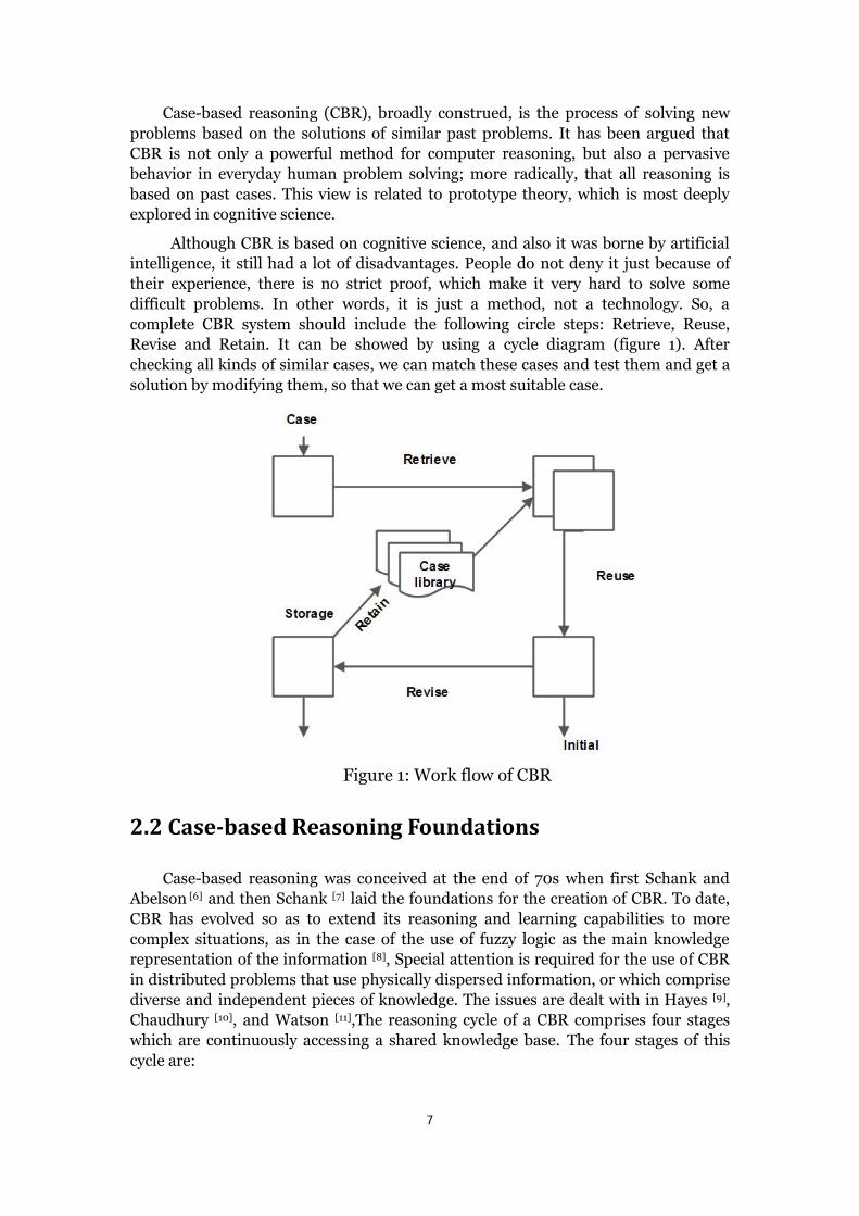
difficult problems. In other words, it is just a method, not a technology. So, a
complete CBR system should include the following circle steps: Retrieve, Reuse,
Revise and Retain. It can be showed by using a cycle diagram (figure 1). After
checking all kinds of similar cases, we can match these cases and test them and get a
solution by modifying them, so that we can get a most suitable case.
Figure 1: Work flow of CBR
2.2 Case-based Reasoning Foundations
Case-based reasoning was conceived at the end of 70s when first Schank and
Abelson [6] and then Schank [7] laid the foundations for the creation of CBR. To date,
CBR has evolved so as to extend its reasoning and learning capabilities to more
complex situations, as in the case of the use of fuzzy logic as the main knowledge
representation of the information [8], Special attention is required for the use of CBR
in distributed problems that use physically dispersed information, or which comprise
diverse and independent pieces of knowledge. The issues are dealt with in Hayes [9],
Chaudhury [10], and Watson [11],The reasoning cycle of a CBR comprises four stages
which are continuously accessing a shared knowledge base. The four stages of this
cycle are:
8
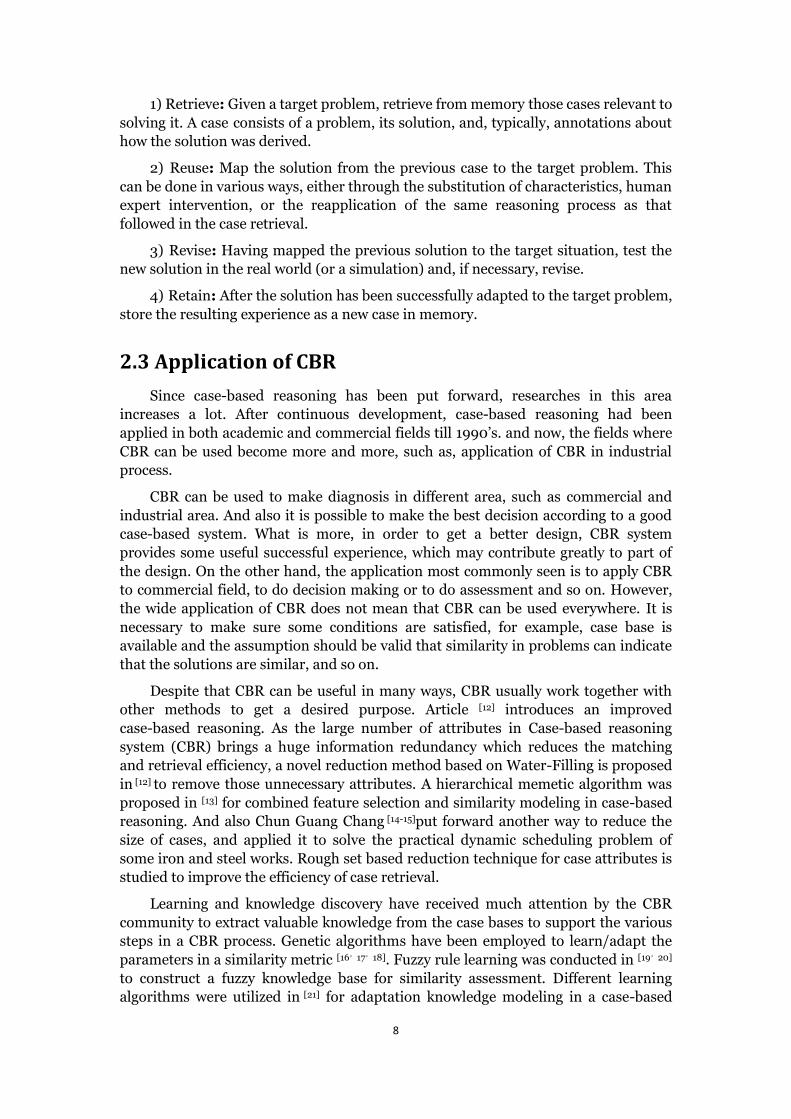
1) Retrieve: Given a target problem, retrieve from memory those cases relevant to
solving it. A case consists of a problem, its solution, and, typically, annotations about
how the solution was derived.
2) Reuse: Map the solution from the previous case to the target problem. This
can be done in various ways, either through the substitution of characteristics, human
expert intervention, or the reapplication of the same reasoning process as that
followed in the case retrieval.
3) Revise: Having mapped the previous solution to the target situation, test the
new solution in the real world (or a simulation) and, if necessary, revise.
4) Retain: After the solution has been successfully adapted to the target problem,
store the resulting experience as a new case in memory.
2.3 Application of CBR
Since case-based reasoning has been put forward, researches in this area
increases a lot. After continuous development, case-based reasoning had been
applied in both academic and commercial fields till 1990’s. and now, the fields where
CBR can be used become more and more, such as, application of CBR in industrial
process.
CBR can be used to make diagnosis in different area, such as commercial and
industrial area. And also it is possible to make the best decision according to a good
case-based system. What is more, in order to get a better design, CBR system
provides some useful successful experience, which may contribute greatly to part of
the design. On the other hand, the application most commonly seen is to apply CBR
to commercial field, to do decision making or to do assessment and so on. However,
the wide application of CBR does not mean that CBR can be used everywhere. It is
necessary to make sure some conditions are satisfied, for example, case base is
available and the assumption should be valid that similarity in problems can indicate
that the solutions are similar, and so on.
Despite that CBR can be useful in many ways, CBR usually work together with
other methods to get a desired purpose. Article [12] introduces an improved
case-based reasoning. As the large number of attributes in Case-based reasoning
system (CBR) brings a huge information redundancy which reduces the matching
and retrieval efficiency, a novel reduction method based on Water-Filling is proposed
in [12] to remove those unnecessary attributes. A hierarchical memetic algorithm was
proposed in [13] for combined feature selection and similarity modeling in case-based
reasoning. And also Chun Guang Chang [14-15]put forward another way to reduce the
size of cases, and applied it to solve the practical dynamic scheduling problem of
some iron and steel works. Rough set based reduction technique for case attributes is
studied to improve the efficiency of case retrieval.
Learning and knowledge discovery have received much attention by the CBR
community to extract valuable knowledge from the case bases to support the various
steps in a CBR process. Genetic algorithms have been employed to learn/adapt the
parameters in a similarity metric [16,17,18]. Fuzzy rule learning was conducted in [19,20]
to construct a fuzzy knowledge base for similarity assessment. Different learning
algorithms were utilized in [21] for adaptation knowledge modeling in a case-based
9
pharmaceutical design task.
3. Algorithm
After considering many aspects, a novel case-based approach is proposed to get
the unsolved real value output. Two main steps for this new algorithm are as follows:
at first, K nearest neighbor regression algorithm is used to add one more attribute to
the original cases, that is, the coefficients of the linear line. Secondly, a new unknown
input attribute x0 remains to be solved. After searching for some useful cases which
already add the coefficient as an input attribute, the output of the new problem can
be calculated in a very easy and time-saving way.
3.1 Off-line Calculation Method
K nearest neighbor algorithm together with regression is applied in the off-line
calculation stage. By using KNN regression, the coefficients for the linear line can be
calculated, which is an important step in this proposed case-based approach.
3.1.1 K Nearest Neighbor Algorithm
K Nearest Neighbor (KNN) algorithm is a classification and prediction method
used widely in pattern recognition and data mining, and it is a supervised machine
learning method. It is also one of the basic technologies in the field of data mining. It
has been proved to be very effective in many fields, but the researches on KNN
algorithm applying for real-valued output are rare relatively.
Given a set of training samples:
{( , ) 1,2, , , ( , ) }p
i i i iS x y i m x y R R
where xi and yi respectively represent input attribute and output, and they are
both real values. Given a sample x0 to be predicted, KNN is used to predict its
associated real-valued output y0 .
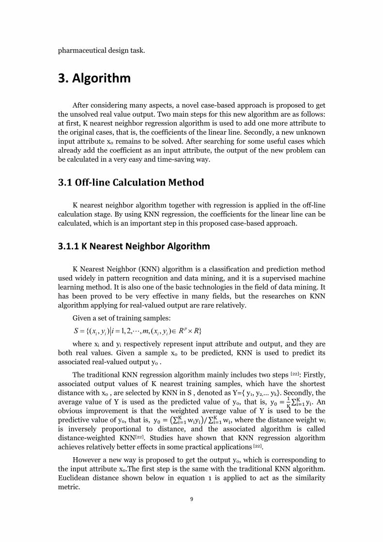
The traditional KNN regression algorithm mainly includes two steps [22]: Firstly,
associated output values of K nearest training samples, which have the shortest
distance with x0 , are selected by KNN in S , denoted as Y={ y1, y2,… yk}. Secondly, the
average value of Y is used as the predicted value of y0, that is,
∑ . An
obvious improvement is that the weighted average value of Y is used to be the
predictive value of y0, that is, (∑ ) ∑
, where the distance weight wi
is inversely proportional to distance, and the associated algorithm is called
distance-weighted KNN[22]. Studies have shown that KNN regression algorithm
achieves relatively better effects in some practical applications [22].
However a new way is proposed to get the output y0, which is corresponding to
the input attribute x0.The first step is the same with the traditional KNN algorithm.
Euclidean distance shown below in equation 1 is applied to act as the similarity
metric.
10
Distance √(x − x )^2 + (x2 − x2 )^2 + …+ (xn − xn )^2 (equation 1)
where x is a n-dimension variable, (x , x2 , ……,xn ) is the input attribute of
the unsolved problem, and (x ,x2 ,…,xn ) is the existing case. By calculating all
the Euclidean distance between the unsolved problem x0 and the known cases in the
dataset, the specified K nearest neighbors can be obtained. On the other hand, the
second step is regression essentially, but some more work has to be done before
applying regression, that is, the following case adaptation part.
3.1.2 Case Adaptation
The major difficulty in case-based reasoning system is the adaptation from
retrieved case. Most of the design problems have to be adapted manually due to the
complexity of the adaptation processes. The approach to make case adaptation varies
much.
The adaptation patterns are the combinations of process parameters, which
would affect the final outcome of a product. A particular process pattern when
observed in a process suggests a good or bad effect in the final product unlike the
traditional adaptation rules, which suggest the amount of change to be made to the
final solution.
In this thesis, from the K neighbors relative to be the nearest to the unsolved
input attribute x0. it is possible to find a method to get the output of this input x0. This
kind of method can be used to get the average value of these neighbors or something
else. However, in this thesis, case adaptation is conducted to get more accurate
information with these limited neighbors. that is, get the incremental value between
two different neighbors. In this way, the useful size of data is increased to Ck2. thus
more accurate information are given by using these limited useful neighbors.
Xnew ∑ ∑ (x − xj) j +
(equation 2)
Ynew ∑ ∑ ( − j) j +
(equation 3)
In the equations above, Xnew and Ynew are vectors to store the adapted cases. And
xi and yi is the obtained cases by using K nearest neighbor algorithm.
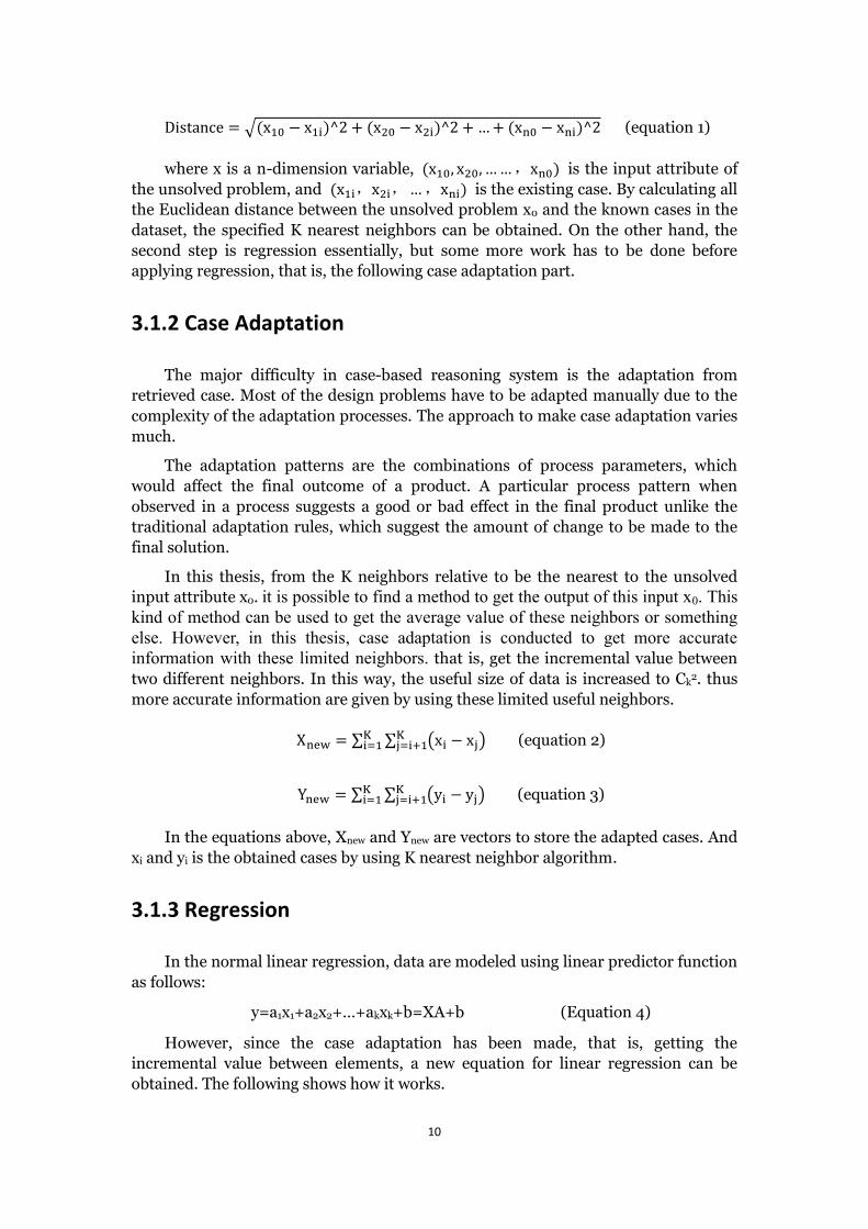
3.1.3 Regression
In the normal linear regression, data are modeled using linear predictor function
as follows:
y=a1x1+a2x2+…+akxk+b=XA+b (Equation 4)
However, since the case adaptation has been made, that is, getting the
incremental value between elements, a new equation for linear regression can be
obtained. The following shows how it works.
11
0 0
0 0
( )y xA b
y y x x Ay x A b
y xA
Y XA
( Equation 5)
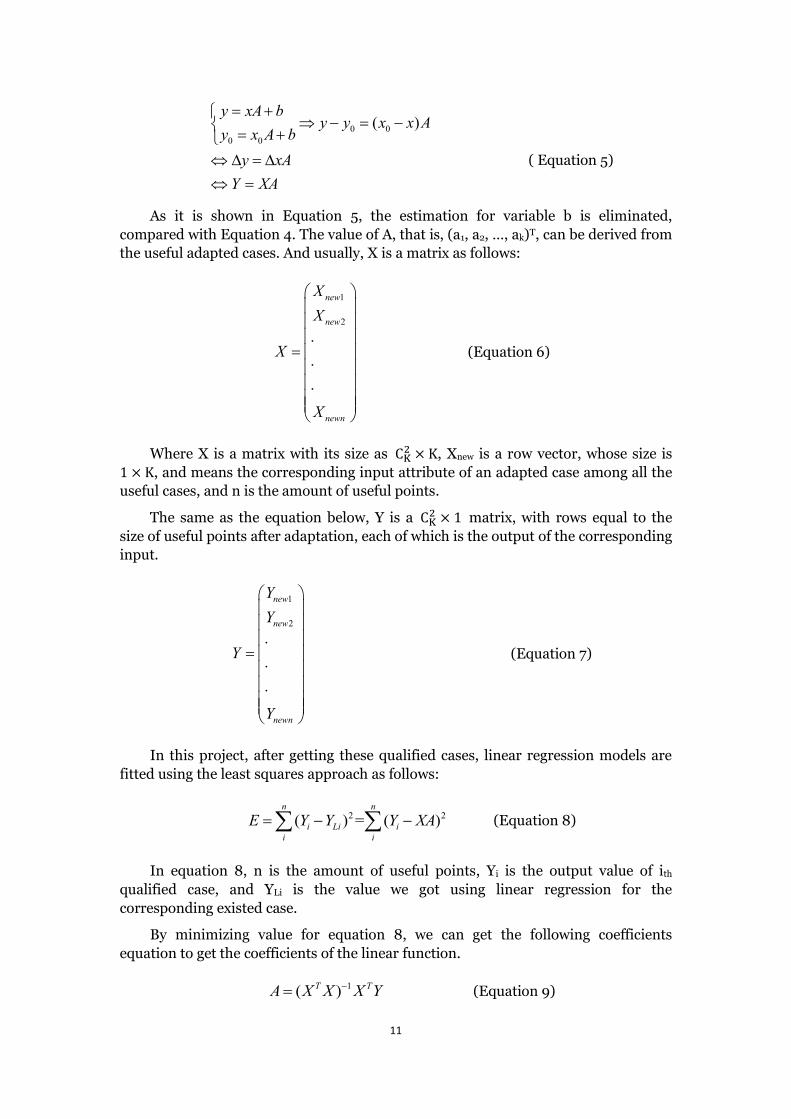
As it is shown in Equation 5, the estimation for variable b is eliminated,
compared with Equation 4. The value of A, that is, (a1, a2, …, ak)T, can be derived from
the useful adapted cases. And usually, X is a matrix as follows:
1
2
new
new
newn
X
X
X
X
(Equation 6)
Where X is a matrix with its size as C 2 × K, Xnew is a row vector, whose size is
1 × K, and means the corresponding input attribute of an adapted case among all the
useful cases, and n is the amount of useful points.
The same as the equation below, Y is a C 2 × 1 matrix, with rows equal to the
size of useful points after adaptation, each of which is the output of the corresponding
input.
1
2
new
new
newn
Y
Y
Y
Y
(Equation 7)
In this project, after getting these qualified cases, linear regression models are
fitted using the least squares approach as follows:
2 2( ) = ( )n n
i Li i
i i
E Y Y Y XA (Equation 8)
In equation 8, n is the amount of useful points, Yi is the output value of ith
qualified case, and YLi is the value we got using linear regression for the
corresponding existed case.
By minimizing value for equation 8, we can get the following coefficients
equation to get the coefficients of the linear function.
1( )T TA X X X Y (Equation 9)

12
As we can see in K nearest neighbor regression method, large quantity of matrix
calculation is really time-consuming. However, all of the time-costing calculation can
be finished before the unsolved problem really comes. The following is about how this
work is done.
Without the real unsolved problem as an input, every time each of the existing
cases in the dataset acts as the unsolved problem. At the same time, all the other
cases act as the training data, thus the desired coefficient for the temporary test case
can be obtained. In this way, with the knowledge of the existing successful cases, each
existing case in the dataset can get one more useful input attribute.
3.2 On-line Calculation Method
After the off-line work has been done, an updated dataset is achieved. Every time
a new problem arrives, instead of large calculation of the K nearest neighbor
regression method mentioned above, the output value can be calculated in a very
simple way with the help of the coefficient attribute. Obviously, this way to deal with
CBR system is much less time-consuming.
On the other hand, it is necessary to understand the reason for the validity and
reliance of this new input attribute. Let us consider two situations: the first situation
is applying K nearest neighbor regression method and calculating everything on-line
when a new problem comes; the second situation can be the approach we put forward
in this article, making some off-line calculation and then get the on-line results. In
the first situation, the new problem is the test case and all the data in the original
dataset are the training data when conducting KNN regression. And coefficients for
the linear line will be calculated and used to get the output value. However, in the
second situation, one of the data in the original dataset acts as the test case, and all
the others are training data. As it can be seen, the only difference between these two
situations when calculating the coefficient attribute is that there is just one case less
in the training data in the second situation compared with the first situation. Usually,
if one case is eliminated from a dataset, which has a pretty large amount of data,
there will not be big difference to the desired results.
To make the output value more accurate, a specified number of neighbors for the
unsolved problem can be found. It is better to take the average value of all the output
of these neighbors.
3.3 some related methods
3.3.1 Average
An average is a measure of the “middle” or “typical” value of a data set. It is thus a
measure of central tendency. In the most common case, the data set is a list of numbers,
13
and the average of a list of numbers is a single number intended to typify the numbers in
the list.
y=(y1+y2+…+yk)/k (Equation 10)
3.3.2 Weighted average
Weighted average is aimed to compute a kind of arithmetic mean of a set of
numbers in which some elements of the set are more important than others. The
influence of different elements in this data set is distinguished by the weighted
coefficient, wi. That is, wi determine the relative importance of each element on the
final average value. Average, or arithmetic mean, is actually a special case of a
weighted average, except all the weights are equal to 1.
y=(w1y1+w2y2+…+wkyk)/(w1+w2+…+wk) (Equation 11)
Here in some part of work in this thesis, the weighted coefficient is related to the
Euclidean distance between this element in the data set with the unsolved element. The
closer they are, the bigger the weighted coefficient is. That is,
1 √(x − x )^2 + (x2 − x2 )^2 + …+ (xn − xn )^2 (Equation 12)
In [23] it was suggested that case similarity degrees being used as the weights to
calculate the weighted average of the outcomes of retrieved cases in prediction for the
new query problem.
4 Ten-fold Cross Validation
Cross-Validation is a statistical method of evaluating and comparing learning
algorithms by dividing data into two segments: one used to learn or train a model and
the other used to validate the model. In typical cross-validation, the training and
validation sets must cross-over in successive rounds such that each data point has a
chance of being validated against. The basic form of cross-validation is k-fold
cross-validation. Other forms of cross-validation are special cases of k-fold
cross-validation or involve repeated rounds of k-fold cross-validation.
Cross-validation is used to evaluate or compare learning algorithms as follows: in
each iteration, one or more learning algorithms use k-1 folds of data to learn one or
more models, and subsequently the learned models are asked to make predictions
about the data in the validation fold. The performance of each learning algorithm on
14
each fold can be tracked using some predetermined performance metric like accuracy.
Upon completion, k samples of the performance metric will be available for each
algorithm. Different methodologies such as averaging can be used to obtain an
aggregate measure from these samples, or these samples can be used in a statistical
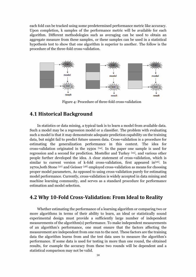
hypothesis test to show that one algorithm is superior to another. The follow is the
procedure of the three-fold cross-validation.
Figure 4: Procedure of three-fold cross-validation
4.1 Historical Background
In statistics or data mining, a typical task is to learn a model from available data.
Such a model may be a regression model or a classifier. The problem with evaluating
such a model is that it may demonstrate adequate prediction capability on the training
data, but might fail to predict future unseen data. Cross-validation is a procedure for
estimating the generalization performance in this context. The idea for
cross-validation originated in the 1930s [24]. In the paper one sample is used for
regression and a second for prediction. Mosteller and Turkey [25], and various other
people further developed the idea. A clear statement of cross-validation, which is
similar to current version of k-fold cross-validation, first appeared in[26]. In
1970s,both Stone [27] and Geisser [28] employed cross-validation as means for choosing
proper model parameters, As opposed to using cross-validation purely for estimating
model performance. Currently, cross-validation is widely accepted in data mining and
machine learning community, and serves as a standard procedure for performance
estimation and model selection.
4.2 Why 10-Fold Cross-Validation: From Ideal to Reality
Whether estimating the performance of a learning algorithm or comparing two or
more algorithms in terms of their ability to learn, an ideal or statistically sound
experimental design must provide a sufficiently large number of independent
measurements of the algorithm(s) performance. To make independent measurements
of an algorithm’s performance, one must ensure that the factors affecting the
measurement are independent from one run to the next. These factors are the training
data the algorithm learns from and the test data uses to measure the algorithm’s
performance. If some data is used for testing in more than one round, the obtained
results, for example the accuracy from these two rounds will be dependent and a
statistical comparison may not be valid.
15
Now the issue becomes selecting an appropriate value for k. A large k is
seemingly desirable, since with a larger k, there are more performance estimates, and
the training set size is closer to the full data size, thus increasing the possibility that
any conclusion made about the learning algorithm(s) under test will generalize to the
case where all the data is used to train the learning model. As k increases, however,
the overlap between training sets also increases. For example, with 5-fold
cross-validation, each training set shares only 3∕4 of its instances with each of the
other four training sets whereas with 10-fold cross-validation, each training set shares
8/9 of its instances with each of the other nine training sets. Furthermore, increasing
k shrinks the size of the test set, leading to less precise, less fine-grained performance
metric. These competing factors have all been considered and the general consensus
in the data mining community seems to be that k = 10 is a good compromise. This
value of k is particularity attractive because it makes predictions using 90% of the
data, making it more likely to be generalizable to the full data.
4.3 Applications of Cross Validation
Cross-validation can be applied in three contexts: performance estimation,
model selection, and tuning learning model parameters. The early uses of
cross-validation were for the investigation of prediction equations but, more recently,
they have been used for model selection purposes. And it also can be used to compare
the performances of different predictive modeling procedures. Many classfiers are
parameterized and their parameters can be tuned to achieve the best result with a
particular dataset. In most cases it is easy to learn the proper value for a parameter
from the available data. Besides it can be performed on the training data as to
measure the performance with each value being tested. Alternatively a portion of the
training set can be reserved for this purpose and not used in the rest of the learning
process. But if the amount of labeled data is limited, this can significantly degrade the
performance of the learned model and cross-validation may be the best option.
5 Implement Procedures
With the help of some graphs, the description below shows how this case-based
approach is fulfilled. All the graph vividly depict how it works in a single input and
single output continuous process. And ten-fold cross validation is used to test the
accuracy.
1. Make use of the existing dataset. The first case in the dataset acts as test case, that
is, the unsolved problem x0. And all the other cases are training data.
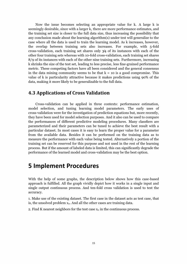
2. Find K nearest neighbors for the test case x0 in the continuous process.
16
x0
X
Y
?
0 2 8-4
X 5 6x0
X0=5.2
0.4
a
b
c
d
e
Figure 2: find K nearest neighbors
3. Make case adaptation. After some incremental calculation, CK2 useful points are
found.
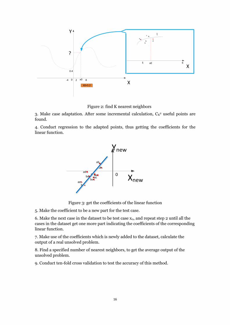
4. Conduct regression to the adapted points, thus getting the coefficients for the
linear function.
Xnew
ab
ac
ad
aebc
bd
be
cd
cede 0
Ynew
Figure 3: get the coefficients of the linear function
5. Make the coefficient to be a new part for the test case.
6. Make the next case in the dataset to be test case x0, and repeat step 2 until all the
cases in the dataset get one more part indicating the coefficients of the corresponding
linear function.
7. Make use of the coefficients which is newly added to the dataset, calculate the
output of a real unsolved problem.
8. Find a specified number of nearest neighbors, to get the average output of the
unsolved problem.
9. Conduct ten-fold cross validation to test the accuracy of this method.
17
6 Experiment tests
The gas furnace datasets is a commonly used benchmark, and it also very useful
in valuation, we compare the results with three different algorithms on this dataset,
these algorithms are applied to estimate the output in a furnace process. Firstly, we
use the simple linear fitting to get the result(square error) comparing with the
method of average and weighted-average, secondly, we add case adaptation to make
the first method more perfect, because this method can make us use less data points
to get the appropriate results, after that we use off-line calculation to subscribe this
online-calculation. In order to make the result more accurate, ten-cross validation is
applied when testing these algorithms.
6.1 Data set
The data set consists of 296 input-output measurements sampled at a fixed
interval of 9 seconds. The measured input u(k) represents the flow rate of the
methane gas in a gas furnace and the output measurement y(k) represents the
concentration of carbon dioxide in the gas mixture flowing out of the furnace under a
steady air supply.
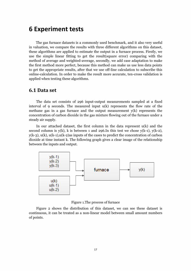
In our attached dataset, the first column in the data represent u(k) and the
second column is y(k), k is between 1 and 296.In this test we chose y(k-1), y(k-2),
y(k-3), u(k), u(k-1),u(k-2)as inputs of the cases to predict the concentration of carbon
dioxide at time instant k. The following graph gives a clear image of the relationship
between the inputs and output.
Figure 1.The process of furnace
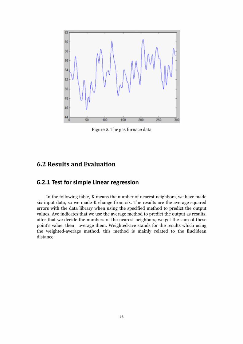
Figure 2 shows the distribution of this dataset, we can see these dataset is
continuous, it can be treated as a non-linear model between small amount numbers
of points.
18
Figure 2. The gas furnace data
6.2 Results and Evaluation
6.2.1 Test for simple Linear regression
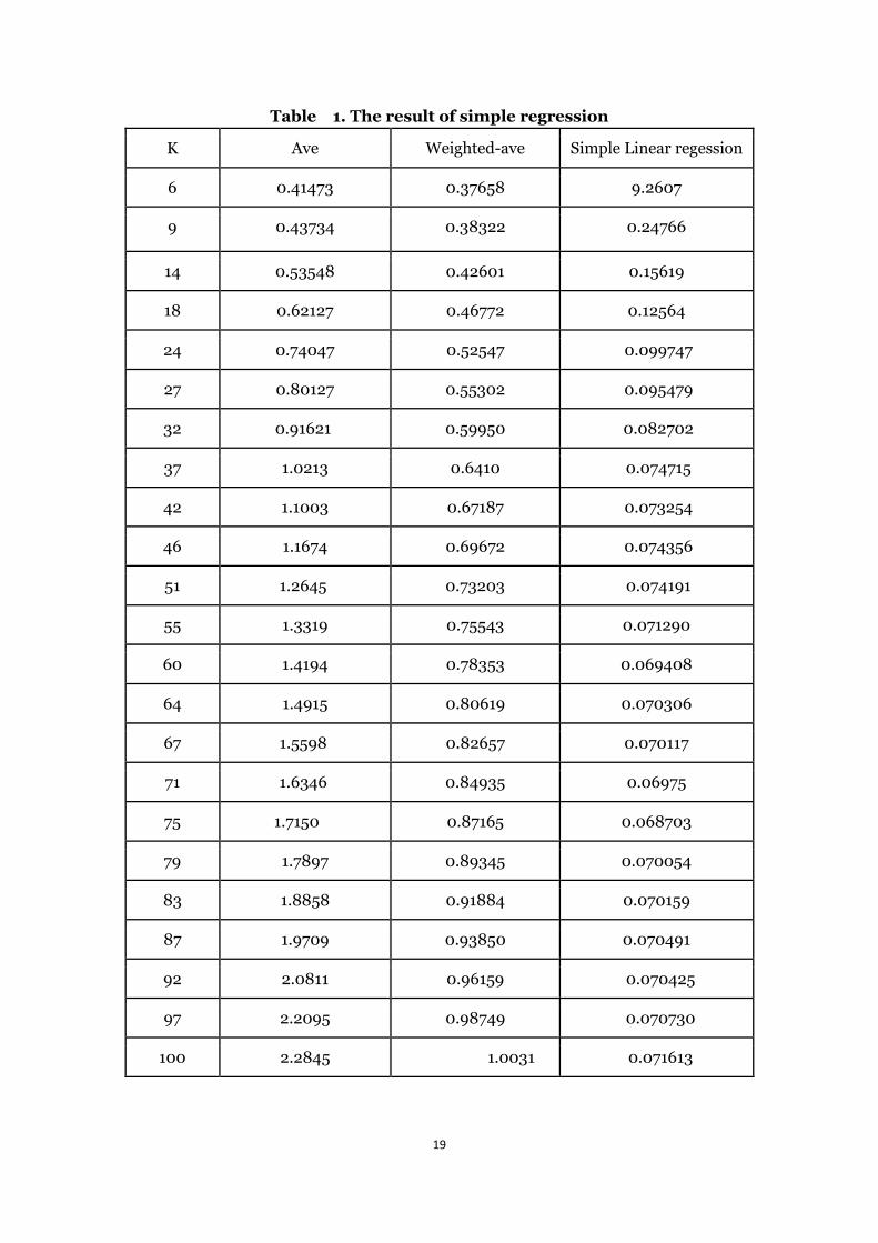
In the following table, K means the number of nearest neighbors, we have made
six input data, so we made K change from six. The results are the average squared
errors with the data library when using the specified method to predict the output
values. Ave indicates that we use the average method to predict the output as results,
after that we decide the numbers of the nearest neighbors, we get the sum of these
point’s value, then average them. Weighted-ave stands for the results which using
the weighted-average method, this method is mainly related to the Euclidean
distance.
19
Table 1. The result of simple regression
K Ave Weighted-ave Simple Linear regession
6 0.41473 0.37658 9.2607
9 0.43734 0.38322 0.24766
14 0.53548 0.42601 0.15619
18 0.62127 0.46772 0.12564
24 0.74047 0.52547 0.099747
27 0.80127 0.55302 0.095479
32 0.91621 0.59950 0.082702
37 1.0213 0.6410 0.074715
42 1.1003 0.67187 0.073254
46 1.1674 0.69672 0.074356
51 1.2645 0.73203 0.074191
55 1.3319 0.75543 0.071290
60 1.4194 0.78353 0.069408
64 1.4915 0.80619 0.070306
67 1.5598 0.82657 0.070117
71 1.6346 0.84935 0.06975
75 1.7150 0.87165 0.068703
79 1.7897 0.89345 0.070054
83 1.8858 0.91884 0.070159
87 1.9709 0.93850 0.070491
92 2.0811 0.96159 0.070425
97 2.2095 0.98749 0.070730
100 2.2845 1.0031 0.071613
20
From the result above, we can see that there are many important factors we
should notice, because they will have a great effect to the result, firstly, with different
amount of neighbors, which is denoted by K, the results vary greatly, for the first
method, when K increase, the result is also turned to increase, but for Simple Linear
regression, when K is small, such as, 6, the error is pretty big, but when k increases
from 6,the error decreases gradually, the larger number the less square error. When
K increase to 75,we can see that the result is the smallest, However, when K continues
to increase, the error becomes larger. The reasons why the error behaves in this way
are explained as follows:
1) When the amount of neighbors is small, the possibility of inaccuracy is much
higher. Since the data library with small number of the nearest neighbor may be not
so concentrated, it is easy to get inaccurate approximation linear line.
2) On the other hand, if the amount of neighbors is too large, it is pointless to
search for the nearest neighbor, because with large number data points, the linear
line will deviate greatly compared to the real line, and we know that linear regression
prove to be very good locally in small interval.
Meanwhile, from the result we can see that the results from simple linear
regression are much better than another two methods(average method and
weighted-average method). So the simple linear regression method is more accurate
than these two methods.
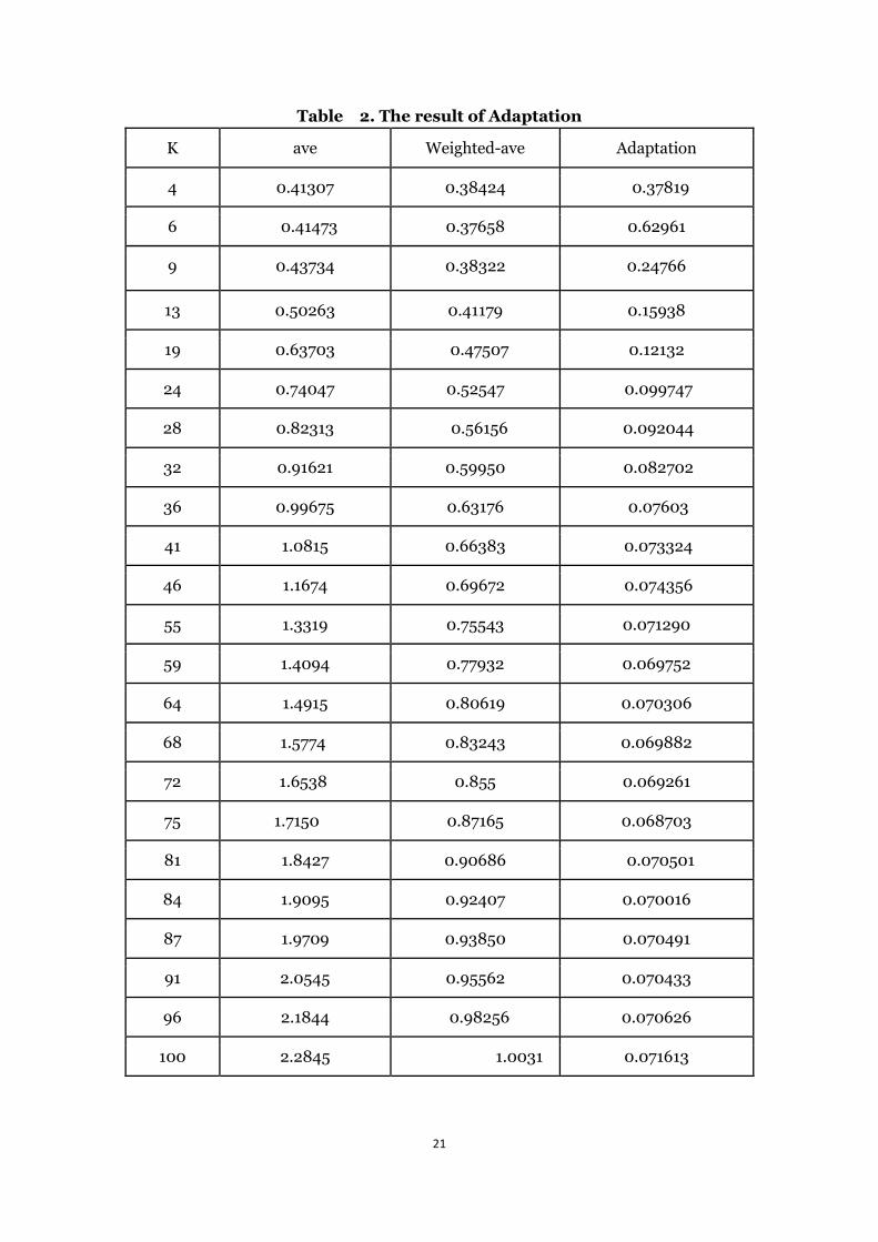
6.2.2 Test for Adaptation
The parameters below (K, ave, Weighted-ave) is the same as above we have
described. For the adaptation part, we just do a little change based on the simple
linear regression, after deciding the number of the nearest neighbor, we don’t use
these data points to do regression directly as last method, firstly making the
adaptation based on these data points, for instance, if we choose four data points,
after the adaptation we can get six data points to do regression, so for the six input
system, the start value of K is four.
21
Table 2. The result of Adaptation
K ave Weighted-ave Adaptation
4 0.41307 0.38424 0.37819
6 0.41473 0.37658 0.62961
9 0.43734 0.38322 0.24766
13 0.50263 0.41179 0.15938
19 0.63703 0.47507 0.12132
24 0.74047 0.52547 0.099747
28 0.82313 0.56156 0.092044
32 0.91621 0.59950 0.082702
36 0.99675 0.63176 0.07603
41 1.0815 0.66383 0.073324
46 1.1674 0.69672 0.074356
55 1.3319 0.75543 0.071290
59 1.4094 0.77932 0.069752
64 1.4915 0.80619 0.070306
68 1.5774 0.83243 0.069882
72 1.6538 0.855 0.069261
75 1.7150 0.87165 0.068703
81 1.8427 0.90686 0.070501
84 1.9095 0.92407 0.070016
87 1.9709 0.93850 0.070491
91 2.0545 0.95562 0.070433
96 2.1844 0.98256 0.070626
100 2.2845 1.0031 0.071613
22
From the result, with the increment of K, the error of first two methods increase
in the meantime, and for adaptation part, the result is same as the simple linear
regression, when K equals 75, the best result comes out.
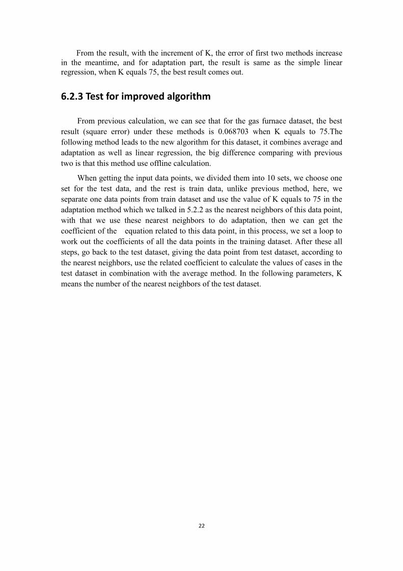
6.2.3 Test for improved algorithm
From previous calculation, we can see that for the gas furnace dataset, the best
result (square error) under these methods is 0.068703 when K equals to 75.The
following method leads to the new algorithm for this dataset, it combines average and
adaptation as well as linear regression, the big difference comparing with previous
two is that this method use offline calculation.
When getting the input data points, we divided them into 10 sets, we choose one
set for the test data, and the rest is train data, unlike previous method, here, we
separate one data points from train dataset and use the value of K equals to 75 in the
adaptation method which we talked in 5.2.2 as the nearest neighbors of this data point,
with that we use these nearest neighbors to do adaptation, then we can get the
coefficient of the equation related to this data point, in this process, we set a loop to
work out the coefficients of all the data points in the training dataset. After these all
steps, go back to the test dataset, giving the data point from test dataset, according to
the nearest neighbors, use the related coefficient to calculate the values of cases in the
test dataset in combination with the average method. In the following parameters, K
means the number of the nearest neighbors of the test dataset.
23
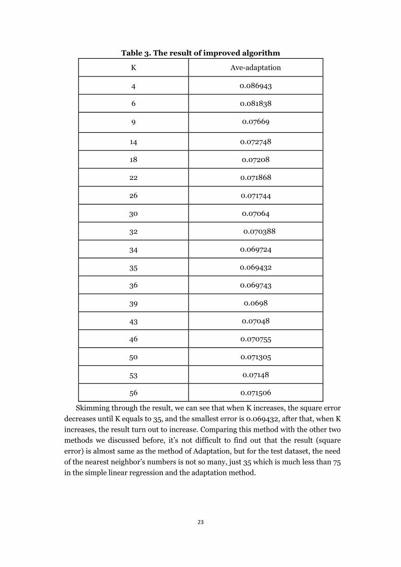
Table 3. The result of improved algorithm
K Ave-adaptation
4 0.086943
6 0.081838
9 0.07669
14 0.072748
18 0.07208
22 0.071868
26 0.071744
30 0.07064
32 0.070388
34 0.069724
35 0.069432
36 0.069743
39 0.0698
43 0.07048
46 0.070755
50 0.071305
53 0.07148
56 0.071506
Skimming through the result, we can see that when K increases, the square error
decreases until K equals to 35, and the smallest error is 0.069432, after that, when K
increases, the result turn out to increase. Comparing this method with the other two
methods we discussed before, it’s not difficult to find out that the result (square
error) is almost same as the method of Adaptation, but for the test dataset, the need
of the nearest neighbor’s numbers is not so many, just 35 which is much less than 75
in the simple linear regression and the adaptation method.
24
7 Summary and Conclusion
After all the test methods, we can see that without designing complicated
mathematical models, CBR can get the desired output with a tolerant error. From the
simple linear regression and adaptation, we can see that the choice of the nearest
neighbor is so important, different value of K will make the result totally different. We
also should notice that the result from the linear regression and adaptation is much
better than the average and weighted-average methods, so these two methods are
more appropriate for this continuous dataset compared with simple average and
weighted-average method.
In the third part, we have presented an operational and a new approach based on
the classical gas furnace dataset in CBR. This method mainly do some changes on the
previous methods(simple linear fitting and adaptation),it combines linear regression
and adaptation with the nearest neighbors, and it also firstly calculate the coefficients
of the equation related to training dataset, so we don’t need to calculate the
coefficients online which is so time-consuming when given the new problem, just use
the coefficients calculated before. Regarding the numbers of the nearest neighbors,
this method gets the best result when K equals 35 instead of 75 in the other two
methods. It use fewer cases to get the best result which is almost the same as the
previous methods. Moreover, this approach has the advantage of being general and
easy to understand and to reuse. In particular, it fits well with the “real world”
applications.
8 Future work
The experiment shows that the approach proposed in this thesis has its own
advantage compared with some other methods. However, there is still some ways to
improve the prediction performance of the CBR system. Due to the time limitation,
we are not able to study it further.
In our opinion, there is at least one improvement for this method. It is possible
and reasonable to make use of some techniques to deal with more complex and high
dimensional dataset. such as, K-means algorithm. In this way, combine clustering
and case-based reasoning is possible to reach better accuracy.
Reference
[1] Schank.R, “Dynamic Memory, A theory of learning in computers and people”,
Cambridge university press,1982.
[2] Kenneth R. Muske, James W. Howse, Glen A.. Hanson et al., Temperature Profile
Estimation for a Thermal Regenerator, Proceeding of the 38th Conference on
Decision and Control, 3944-3949, 1998.
25
[3] Huang Zhaojun, Bai Fengshuang, Zhuang Bin et al., Flow Set and Control Expert
System of Hot Stoves for Blast Furnace, Metallurgical Automation, Vol.26, No.5,
38-40, 2002.
[4] Ma Zhuwu, Lou Shengqiang, Li Gang et al., The Intelligence Burning Control of
the Hot Stove of Lianyuan Iron & Steel Group Co., Metallurgical Automation, Vol.26,
No.4, 11-15, 2002.
[5] Sun Jinsheng, Research on a Case-Based Reasoning AI Control Strategy for Blast
Furnace Stove Combustion, Doctor Thesis, China University of Mining and
Technology, 2005.
[6] R.Schank, R. Abelson, Script, Plans, Goals and Understanding, Hillsdale, NJ:
Erlbaum, 1977.
[7] R.Schank, Dynamic Memory: A Theory of Learning in Computers and People,
Cambridge University Press, New York, 1982.
[8] H.Li,S Dick.A similarity measure for fuzzy rrlebases based on linguistic gradients.
Information Science 176, 2006, pp.2960-2987.
[9] C.Hayes, C., P. Cunningham, P., M. Doyle, M.Distributed CBR using XML
(Department of Computer Science Trinity College, Dublin)2001.
[10] S.Chaudhury, T.Singh, P.S.Goswami. Distributed fuzzy case based reasoning.
Applied Soft Computing,4, 2004, pp.323-343.
[11] I.Watson, D. Gardingen, “A Distributed Case Based Reasoning Application for
Engineering Sales Support”. In Procc. of the IJCAI-99, 1999, pp. 600-605.
[12] Hui Zhao, Ai-jun Yan, Chun-xiao Zhang and Pu Wang, Attribute Reduction
Method Using Water-filling Principle for Case-based Reasoning. Proceedings of the
10th World Congress on Intelligent Control and Automation. July 6-8, 2012, Beijing,
China.
[13] N. Xiong, and P. Funk, “Combined feature selection and similarity modeling in
case-based reasoning using hierarchical memetic algorithm”, In: Proceedings of the
IEEE World Congress on Computational Intelligence, 2010, pp. 1537-1542.
[14] Chun Guang Chang, Ding Wei Wang, Kun Yuan Hu, Zhi Tao., Study on rough set
based reduction technique for case attributes, proceedings of the Third International
Conference on Machine Learning and Cybernetics, shanghai, 26-29, August 2004.
[15] J. W. Han, and M. Kamber, “Data Mining: Concepts and Techniques,” China
Machine Press, 2007, Beijing.
[16] H. Ahn, K. Kim, and I. Han, “Global optimization of feature weights and the
number of neighbors that combine in a case-based reasoning system,” Expert
Systems, vol. 23, pp. 290-301, 2006.
[17] J. Jarmulak, S. Craw, and R. Rowe, “Genetic algorithms to optimize CBR
retrieval,” In: Proc.European Workshop on Case-Based Reasoning (EWCBR 2000),
2000, pp. 136-147.
[18] N. Xiong, “Towards coherent matching in case-based classification”, Cybernetics
and Systems, Vol. 42, 2011, pp. 198-214.
[19] N. Xiong, “Learning fuzzy Rules for similarity assessment in case-based
reasoning”, Expert Systems and Applications, Vol 38, 2011, pp. 10780-10786.
26
[20] N. Xiong, “Fuzzy rule-based similarity model enables learning from small case
bases,” Applied Soft Computing, vol. 13, pp. 2057-2064, 2013.
[21] S. Craw, N. Wiratunga, and R. C. Rowe, Learning adaptation knowledge to
improve case-based reasoning, Artificial Intelligence, Vol. 170, 2006, pp. 1175-1192.
[22] T. Ye, X. F. Zhu, X. Y. Li, and B. H. Shi, “Soft sensor modeling based on a
modified k-nearest neighbor regression algorithm,” Acta Automatica Sinica. 2007, vol.
33, pp. 996–999.
[23] N. Xiong, and P. Funk, “Building similarity metrics reflecting utility in
case-based reasoning”, Journal of Intelligent and Fuzzy Systems, Vol. 17, No. 4,
2006, pp. 407-416.
[24] Larson S.The shrinkage of the coefficient of multiple correlation. J. Educat.
Psychol., 22:45–55,1931.
[25] Mosteller F.and Wallace D.L.Inference in an authorship problem. J. Am. Stat.
Assoc,58:275–309, 1963.
[26]Mosteller F. and Turkey J.W. Data analysis, including statistics. In Handbook of
Social Psychology. Addison-Wesley, Reading,MA, 1968.
[27] Stone M. Cross-validatory choice and assessment of statistical predictions. J.
Royal Stat. Soc., 36(2):111–147,1974.
[28] Geisser S. The predictive sample reuse method with applications. J. Am. Stat.
Assoc., 70(350):320–328,1975.