Case Study: HDM-4 adaptation for analyzing Kenya roads

Jennaro B. Odoki

131 Swarthmore Road Selly Oak

Birmingham B29 4NN

United Kingdom

Email: jennarodoki@yahoo.co.uk

ACRONYMS AND ABBREVIATIONS AADT – Annual Average Daily Traffic BCR - Benefit Cost Ratio ESALF - Equivalent Standard Axle Load Factor FYRR - First Year Rate of Return HDM-4 - Highway Development and Management Tool IQL - Information Quality Level IRI - International Roughness Index IRR - Internal Rate of Return KeNHA - Kenya National Highways Authority KeRRA - Kenya Rural Roads Authority KRB - Kenya Roads Board KURA - Kenya Urban Roads Authority KWS - Kenya Wildlife Services MCA - Multi-Criteria Analysis MT - Motorized Transport MOTI - Ministry of Transport and Infrastructure MTRD - Materials Testing and Research Department NMT - Non-motorized Transport NPV - Net Present Value NTSA - National Transport and Safety Authority PCSE - Passenger Car Space Equivalent RAC - Road Agency Cost RSIP - Road Sector Investment Programme RSIP TF - Road Sector Investment Programme Task Force RUC - Road User Cost RUE - Road User Effects VOC - Vehicle Operating Costs

1

1 Introduction

This paper presents a case study to adapt the highway development and

management tool (HDM-4) for investigating road investment choices in Kenya.

Roads constitute the most important mode of transport in Kenya since more than

93% of all freight and passenger traffic is transported by road. Kenya’s public

road network comprises some 161,451km of which 14,561km is paved while

146,890km is unpaved. The estimated value of the road asset is KShs 2.5 trillion

and this represents a significant portion of the country’s public investments.

Given its contribution to the country’s socioeconomic development and the

public investment it represents, the roads network must be continuously

developed, managed and maintained in a prudent and effective manner.

There is currently a widespread recognition in Kenya of the importance of road

development and maintenance and the value placed on the issue both by users

and the wider community. There is also an increasing understanding of the

serious consequences of failure to invest adequately and effectively in

maintaining the national road network. For this reason, the Government of

Kenya desires to have an objective and scientific system to assist decision-makers

in the allocation of resources for road maintenance and development that is

consistent with the actual needs of the road network. It also wants to have better

appreciation of the effect of various investment levels and its long-term impact

on the condition of the road network, the road users and the environment. In the

allocation of resources, there is need to have a mechanism that ensures optimum

and equitable distribution that avoids skewedness to any class or type of road

within the network. In the face of scarce resources, the determination of road

investment priorities that yield maximum returns to the economy of Kenya is

also of concern to the Government.

2

The adoption of HDM-4 by the Ministry of Transport and Infrastructure and its

agencies is therefore aimed at improving decision-making on expenditures in the

road sector by enabling effective and sustainable utilisation of the latest Highway

Development and Management (HDM-4) knowledge.

This case study constitutes a broader assignment commissioned by Kenya Roads

Board (KRB) with the following objectives:

(i) To improve the configuration and calibration parameters of HDM-4

Kenyan Workspace. The update of configuration and calibration

parameters will be done for the latest version of HDM-4 (Version 2.08).

(ii) In close consultation with the Road Sector Investment Programme Task

Force (RSIP TF), develop a detailed short term 5 year Road Sector

Investment Programme (2015 – 2019) anchored on long term sector plans

(including the 15 year RSIP) and national priorities.

2 HDM-4 Analytical Framework

2.1 Introduction

The basic unit of analysis in HDM-4 is the homogeneous road section. Several

investment options can be assigned to a road section for analysis. The vehicle

types that use the road must also be defined together with the traffic volume

specified in terms of the annual average daily traffic (AADT).

The analytical framework of HDM-4 is based on the concept of pavement life

cycle analysis, which is typically 15 to 40 years depending on the pavement type.

This is applied to predict road deterioration (RD), road works effects (WE), road

user effects (RUE), and socio-economic and environmental effects (SEE) (Odoki

and Kerali, 2006). The underlying operation of HDM-4 is common for the project,

programme or strategy applications. In each case, HDM-4 predicts the life cycle

pavement performance and the resulting user costs under specified maintenance

3

and/or road improvement scenarios. The agency and user costs (i.e. RAC and

RUC, respectively) are determined by first predicting physical quantities of

resource consumption and then multiplying these by the corresponding unit

costs.

Two or more options comprising different road maintenance and/or

improvement works should be specified for each candidate road section with one

option designated as the base case (usually representing minimal routine

maintenance). The benefits derived from implementation of other options are

calculated over a specified analysis period by comparing the predicted economic

cost streams in each year against that for the respective year of the base case

option. The discounted total economic cost difference is defined as the net

present value (NPV). Other economic indicators calculated are the internal rate

of return (IRR), benefit-cost ratio (BCR) and first year rate of return (FYRR). The

average life cycle riding quality measured in terms of the international roughness

index (IRI) is also calculated for each option.

2.2 Overall Logic Sequence

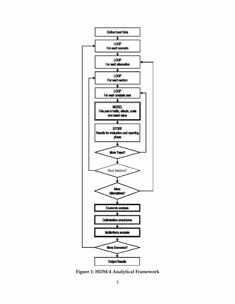
The overall logic sequence for economic analysis and optimisation is illustrated

in Figure 1. This figure shows the following (Odoki and Kerali, 2006):

The outer analysis loop - enables economic comparisons to be made for each pair of

investment options, using the effects and costs calculated over the analysis

period for each option, and it allows for variations in generated and diverted

traffic levels depending on the investment option considered.

The inner analysis loop – shows how annual effects and costs to the road agency

and to the road users, and asset values are calculated for individual road section

options.

Optimisation procedures and budget scenario analysis - these are performed after

economic benefits of all the section options have been determined.

4

Multiple criteria analysis (MCA) - provides a means of comparing investment

options using criteria that cannot easily be assigned an economic cost. Note that

this capability has not been used in the present study.

2.3 Data Requirements

The main data sets required as inputs for HDM-4 analyses are categorised as

follows (Kerali et al., 2000):

(i) Road network data comprising: inventory, geometry, pavement type,

pavement strength, and road condition defined by different distress

modes;

(ii) Vehicle fleet data including vehicle physical and loading characteristics,

utilisation and service life, performance characteristics such as driving

power and braking power, and unit costs of vehicle resources;

(iii) Traffic data including details of composition, volumes and growth rates,

speed-flow types and hourly traffic flow pattern on each road section;

(iv) Road works data comprising historical records of works performed on

different road sections, a range of road maintenance activities practised in

the country and their associated unit costs.

(v) Economic analysis parameters including time values, discount rate and base

year.

5

Figure 1: HDM-4 Analytical Framework

6

2.4 Reliability of results

The reliability of the results obtained from HDM-4 analysis is dependent upon

two primary considerations (Bennett and Paterson, 2000):

How well the data provided to the model represent the reality of current

conditions and influencing factors, in the terms understood by the model;

and,

How well the predictions of the model fit the real behavior and the

interactions between various factors for the variety of conditions to which

it is applied.

Application of the model thus involves two important steps:

(i) Data input: a correct interpretation of the data input requirements, and

achieving a quality of input data that is appropriate to the desired

reliability of the results.

(ii) Calibration of outputs: adjusting the model parameters to enhance how well

the forecast and outputs represent the changes and influences over time

and under various interventions in Kenya. Calibration of the HDM model

focuses on the components that determine the physical quantities, costs

and benefits predicted for the Road Deterioration and Works Effects

(RDWE), Road User Effects (RUE), Traffic Characteristics and Socio-

Economic Effects (SEE) analysis.

The accuracy required of the input data is dictated by the objectives of the

analysis. For a very approximate analysis there is no need to quantify the input

data to a very high degree of accuracy. Conversely, for a detailed analysis it is

important to quantify the data as accurately as is practical given the available

resources.

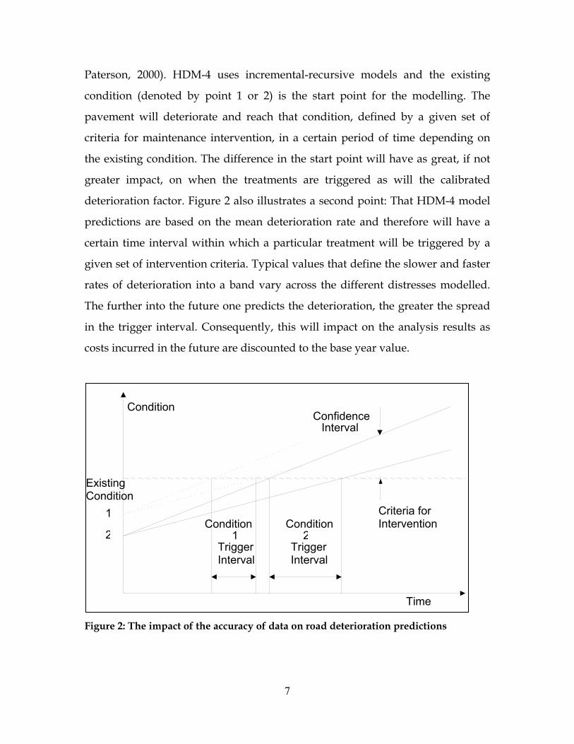
Figure 2 illustrates the impact of the accuracy of input data on road deterioration

predictions and the timing of future maintenance interventions (Bennett and

7

Paterson, 2000). HDM-4 uses incremental-recursive models and the existing

condition (denoted by point 1 or 2) is the start point for the modelling. The

pavement will deteriorate and reach that condition, defined by a given set of

criteria for maintenance intervention, in a certain period of time depending on

the existing condition. The difference in the start point will have as great, if not

greater impact, on when the treatments are triggered as will the calibrated

deterioration factor. Figure 2 also illustrates a second point: That HDM-4 model

predictions are based on the mean deterioration rate and therefore will have a

certain time interval within which a particular treatment will be triggered by a

given set of intervention criteria. Typical values that define the slower and faster

rates of deterioration into a band vary across the different distresses modelled.

The further into the future one predicts the deterioration, the greater the spread

in the trigger interval. Consequently, this will impact on the analysis results as

costs incurred in the future are discounted to the base year value.

Figure 2: The impact of the accuracy of data on road deterioration predictions

Time

Condition

Existing Condition

Confidence Interval

Criteria for Intervention

1

2Condition

2Trigger Interval

Condition1

Trigger Interval

8

3 Configuration and Calibration of HDM-4

The adaptation of HDM-4 for analysing Kenya roads involves two major

activities: configuration and calibration. Each of these is outlined below. Prior to

using HDM-4 for the first time in any country, the system should be configured

and calibrated for local use.

3.1 Configuration

The primary objective of configuration is to make the analysis from the model

relevant and compatible to the environment in Kenya by restructuring default

configuration data in line with local conditions, standards and practices. HDM-4

configuration shall involve a number of activities that include the following:

(i) Provision of information on the climatic conditions prevailing in Kenya,

different road types and functional classes, and the pavement types that

constitute the road network.

(ii) Definition of the general characteristics of traffic flow on the different road

types in the network; the traffic bands, traffic composition by

representative vehicle types and traffic growth rates pertaining to each

road type/class. Types of accidents predominant on each road type and

accident rates have to be determined.

(iii) Definition of road surface condition in aggregate form (e.g. good, fair,

poor) based on measures of surface distresses (e.g. cracking, ravelling,

rutting, potholes, edgebreak, roughness, thickness of gravel) to conform to

local standards and practices.

(iv) General assessment of quality of road construction in Kenya using strict

adherence to technical specifications and design standards as a measure of

full compliance in order to reflect local quality control regime.

(v) Estimation of pavements strength of the various road types and classes

expressed in terms of structural number and deflection.

9

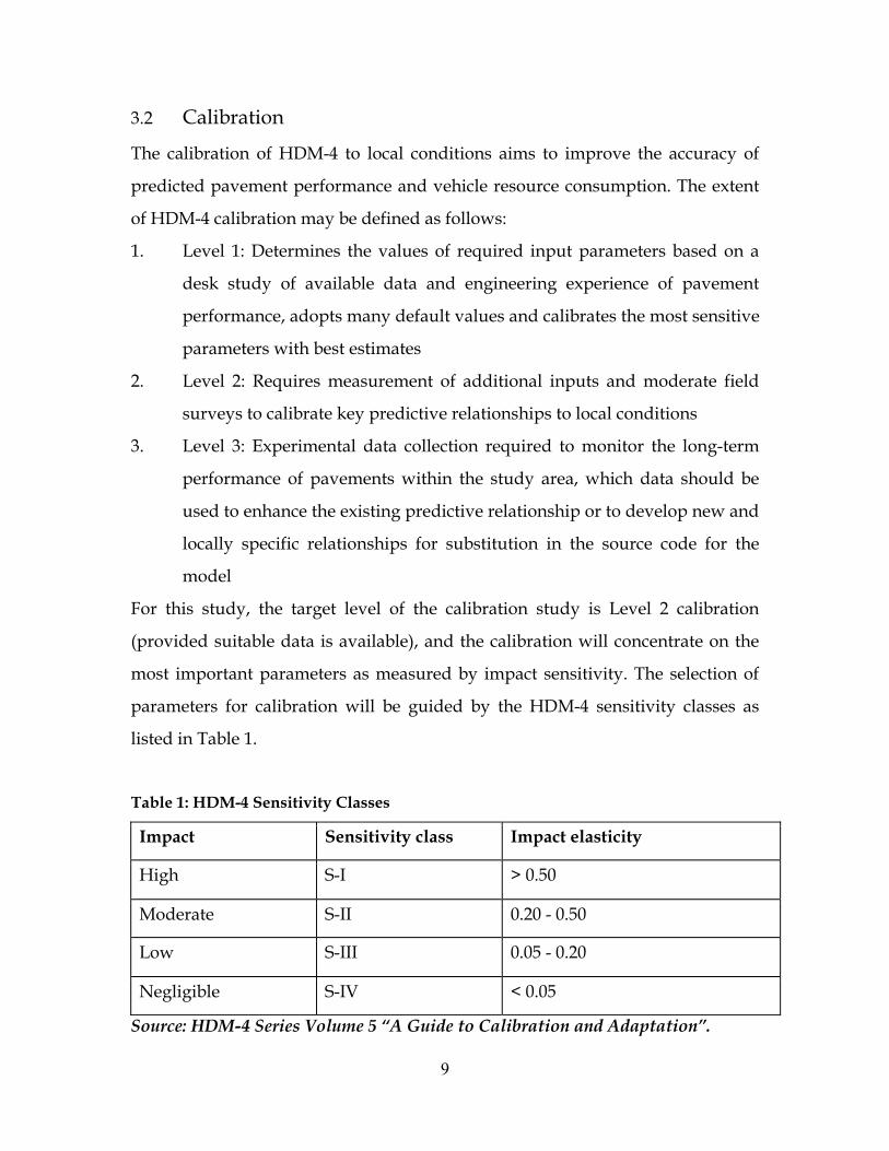
3.2 Calibration

The calibration of HDM-4 to local conditions aims to improve the accuracy of

predicted pavement performance and vehicle resource consumption. The extent

of HDM-4 calibration may be defined as follows:

1. Level 1: Determines the values of required input parameters based on a

desk study of available data and engineering experience of pavement

performance, adopts many default values and calibrates the most sensitive

parameters with best estimates

2. Level 2: Requires measurement of additional inputs and moderate field

surveys to calibrate key predictive relationships to local conditions

3. Level 3: Experimental data collection required to monitor the long-term

performance of pavements within the study area, which data should be

used to enhance the existing predictive relationship or to develop new and

locally specific relationships for substitution in the source code for the

model

For this study, the target level of the calibration study is Level 2 calibration

(provided suitable data is available), and the calibration will concentrate on the

most important parameters as measured by impact sensitivity. The selection of

parameters for calibration will be guided by the HDM-4 sensitivity classes as

listed in Table 1.

Table 1: HDM-4 Sensitivity Classes

Impact Sensitivity class Impact elasticity

High S-I > 0.50

Moderate S-II 0.20 - 0.50

Low S-III 0.05 - 0.20

Negligible S-IV < 0.05

Source: HDM-4 Series Volume 5 “A Guide to Calibration and Adaptation”.

10

In identifying data to be collected, HDM-4 Volume 5 documentation series

provides guidance which recommends that efforts should be based on the results

of these sensitivity analyses. Those data items or model coefficients with

moderate to high impacts (S-I and S-II) should receive the most attention. The

low to negligible impact (S-III and S-IV) items should receive attention only if

time or resources permit.

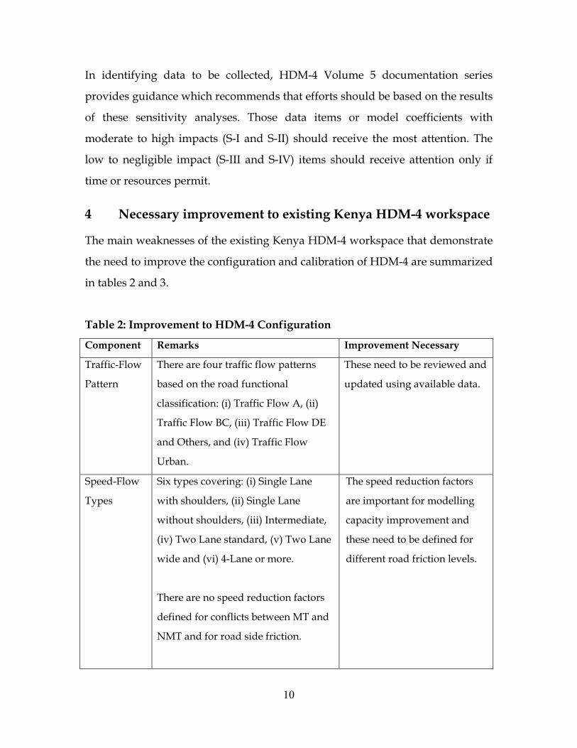
4 Necessary improvement to existing Kenya HDM-4 workspace

The main weaknesses of the existing Kenya HDM-4 workspace that demonstrate

the need to improve the configuration and calibration of HDM-4 are summarized

in tables 2 and 3.

Table 2: Improvement to HDM-4 Configuration

Component Remarks Improvement Necessary

Traffic-Flow

Pattern

There are four traffic flow patterns

based on the road functional

classification: (i) Traffic Flow A, (ii)

Traffic Flow BC, (iii) Traffic Flow DE

and Others, and (iv) Traffic Flow

Urban.

These need to be reviewed and

updated using available data.

Speed-Flow

Types

Six types covering: (i) Single Lane

with shoulders, (ii) Single Lane

without shoulders, (iii) Intermediate,

(iv) Two Lane standard, (v) Two Lane

wide and (vi) 4-Lane or more.

There are no speed reduction factors

defined for conflicts between MT and

NMT and for road side friction.

The speed reduction factors

are important for modelling

capacity improvement and

these need to be defined for

different road friction levels.

11

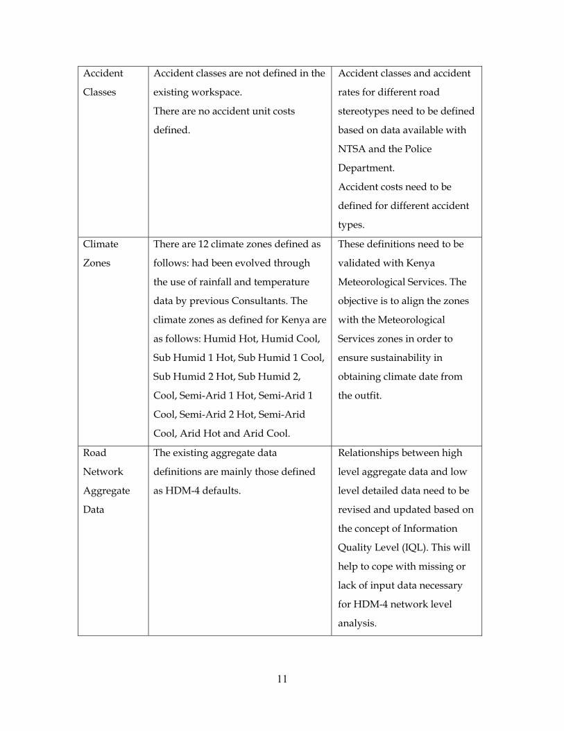
Accident

Classes

Accident classes are not defined in the

existing workspace.

There are no accident unit costs

defined.

Accident classes and accident

rates for different road

stereotypes need to be defined

based on data available with

NTSA and the Police

Department.

Accident costs need to be

defined for different accident

types.

Climate

Zones

There are 12 climate zones defined as

follows: had been evolved through

the use of rainfall and temperature

data by previous Consultants. The

climate zones as defined for Kenya are

as follows: Humid Hot, Humid Cool,

Sub Humid 1 Hot, Sub Humid 1 Cool,

Sub Humid 2 Hot, Sub Humid 2,

Cool, Semi-Arid 1 Hot, Semi-Arid 1

Cool, Semi-Arid 2 Hot, Semi-Arid

Cool, Arid Hot and Arid Cool.

These definitions need to be

validated with Kenya

Meteorological Services. The

objective is to align the zones

with the Meteorological

Services zones in order to

ensure sustainability in

obtaining climate date from

the outfit.

Road

Network

Aggregate

Data

The existing aggregate data

definitions are mainly those defined

as HDM-4 defaults.

Relationships between high

level aggregate data and low

level detailed data need to be

revised and updated based on

the concept of Information

Quality Level (IQL). This will

help to cope with missing or

lack of input data necessary

for HDM-4 network level

analysis.

12

Table 3: Improvement to HDM-4 Model Calibration

Component Remarks Improvement Necessary

Road

Deterioration

The workspace does not

include reasonable calibrated

road deterioration (RD)

model and calibration sets.

The RD models need to be

calibrated in order to accurately

predict the deterioration trends of

different pavement types in Kenya.

Works Standards

and Effects

There are no optimal work

standards derived for

different road functional

classes.

Optimal work standards need to be

defined.

Unit costs of various work

activities are not defined in the

Work Standard.

Road User Effects Road user effects models

have been calibrated in a

study conducted in 2011.

Unit costs of various vehicle

resource consumption need to be

updated.

Table 4 summarizes other areas that warrant improvement to Kenya HDM-4

Workspace.

Table 4: Improvement to Other HDM-4 Workspace Data

Component Remarks Improvement Necessary

Vehicle Fleet Kenya has the following 10

vehicle classes: Car, 4WD & Jeep,

Pick-up Utility, Mini- bus

(Matatu), Small Bus, Large Bus,

Light Truck, Medium Truck,

Heavy Truck, Articulated Truck

The values of equivalent

standard axle load factors

(ESALF) given in the

workspace are not correct.

There are no Non-Motorised

Transport defined in the

Vehicle Fleet reviewed. NMT

need to be included.

Representative traffic growth

rates need to be defined.

13

Worked

Examples of

Typical Case

Studies

Only HDM-4 default case studies

are available.

Typical case studies relevant to

Kenya road network

development and maintenance

are not included.

Furthermore, there is no HDM-4 workspace to model roads under Kenya

Wildlife Services (KWS). KWS will have to provide inventory of the road

network they manage in a excel spreadsheet format. This together with the

workspaces for KeRRA, KURA and KeNHA will be used to prepare a

consolidated HDM-4 workspace to be used in the preparation of the RSIP.

5 Study Approach and Methodology

5.1 HDM-4 Configuration

Traffic Flow Patterns

The levels of traffic congestion vary with the hour of the day and on different

days of the week and year. To take account of this, the number of hours of the

year for which different ranges of hourly flows are applicable will be determined

from the data that will be collected. To configure traffic flow pattern, the

distribution of hourly flows over 8760 hours of the year will be defined for each

road use type based on available data from the road agencies.

Speed-Flow and Speed Reduction Factors

The speed-flow model adopted in HDM-4 for motorised transport (MT) is the

three-zone model illustrated in Figure 3. Motorised vehicle speeds and operating

resources are determined as functions of the characteristics of each type of

vehicle and the geometry, surface type and current condition of the road, under

both free flow and congested traffic conditions.

14

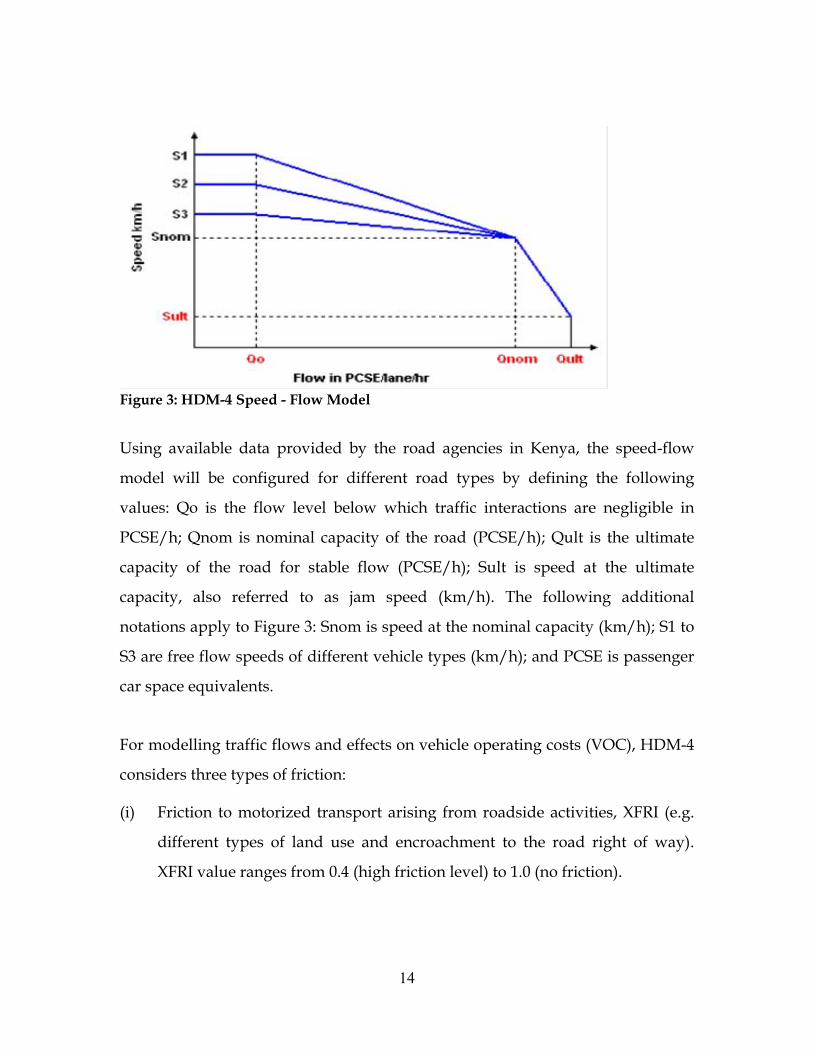
Figure 3: HDM-4 Speed - Flow Model

Using available data provided by the road agencies in Kenya, the speed-flow

model will be configured for different road types by defining the following

values: Qo is the flow level below which traffic interactions are negligible in

PCSE/h; Qnom is nominal capacity of the road (PCSE/h); Qult is the ultimate

capacity of the road for stable flow (PCSE/h); Sult is speed at the ultimate

capacity, also referred to as jam speed (km/h). The following additional

notations apply to Figure 3: Snom is speed at the nominal capacity (km/h); S1 to

S3 are free flow speeds of different vehicle types (km/h); and PCSE is passenger

car space equivalents.

For modelling traffic flows and effects on vehicle operating costs (VOC), HDM-4

considers three types of friction:

(i) Friction to motorized transport arising from roadside activities, XFRI (e.g.

different types of land use and encroachment to the road right of way).

XFRI value ranges from 0.4 (high friction level) to 1.0 (no friction).

15

(ii) Friction to motorized transport due to the presence of non-motorised

transport XNMT (e.g. pedestrians, bicycles, animal carts). XNMT value

ranges from 0.4 (high friction level) to 1.0 (no friction).

(iii) Friction to non-motorized transport arising from motorized transport using

the road, XMT. Values of XMT also range from 0.4 to 1.0.

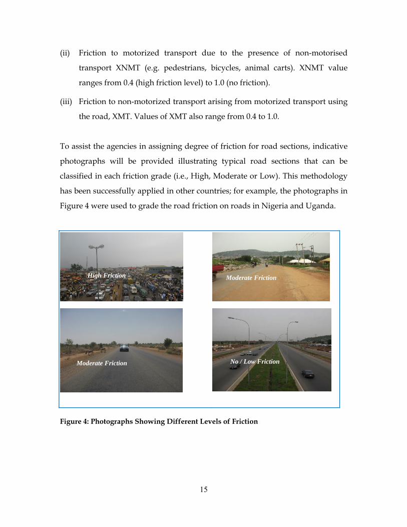
To assist the agencies in assigning degree of friction for road sections, indicative

photographs will be provided illustrating typical road sections that can be

classified in each friction grade (i.e., High, Moderate or Low). This methodology

has been successfully applied in other countries; for example, the photographs in

Figure 4 were used to grade the road friction on roads in Nigeria and Uganda.

Figure 4: Photographs Showing Different Levels of Friction

High Friction Moderate Friction

Moderate Friction No / Low Friction

16

Accident Classes, Rates and Costs

Accident rates for road stereotypes will be determined using data from the

Kenya Police Service records, the National Transport and Safety Authority

(NTSA) and other sources. Accident rates in ‘number per 100 million vehicle

kilometres’ will be determined for the following categories of accidents modelled

in HDM-4: fatal accidents; injury; and damage only accidents. Accident rates for

each severity vary with parameters like road type, traffic level and flow-pattern,

the presence of non-motorized transport, road geometry, and road surface

characteristics.

Although it is not easy to attribute monetary values to the losses arising from

accidents, estimates of accident costs are essential aid to decision-making in the

road safety aspects and investment choices. Costs of road accidents arise from

the following areas, TRL (2005):

Damage to vehicles and other property

Costs of hospital treatment, police work, administration, etc.

Loss of life and injury

The first two areas of losses involve material resources and are normally readily

defined, even though their values may be uncertain. They can be translated into

economic terms without great difficulty. Costs relating to the loss of life and

injury are subjective, involving the need to value human life and ‘pain, grief and

suffering’. The valuing of human life is a difficult and often contentious process.

Several methods of valuing human life exist including the gross output, net

output, life insurance, court award, value of risk-charge, and implicit public

sector valuation. Different accident cost methodologies will be investigated in

order to select those that are relevant to the objectives being pursued taking into

consideration data availability and quality in Kenya.

17

Climate Zones

Existing HDM-4 workspaces used by the road agencies in Kenya have input for

the Climate Zone. Twelve climate zones have been defined for Kenya based on

temperature classification and moisture regime. These need to be reviewed using

new data from Kenya Meteorological Department and literature with the aim of

rationalizing the number of climate zones relative to the degree of accuracy

required by HDM-4 analysis. For each climate zone, the following parameters

will be reviewed and if found necessary updated: moisture Index; duration of

dry season as a percentage of the year; mean temperature; number of days with

temperature greater than 35 degrees Celsius; freeze index; and percentage of

time vehicles are driven on wet roads.

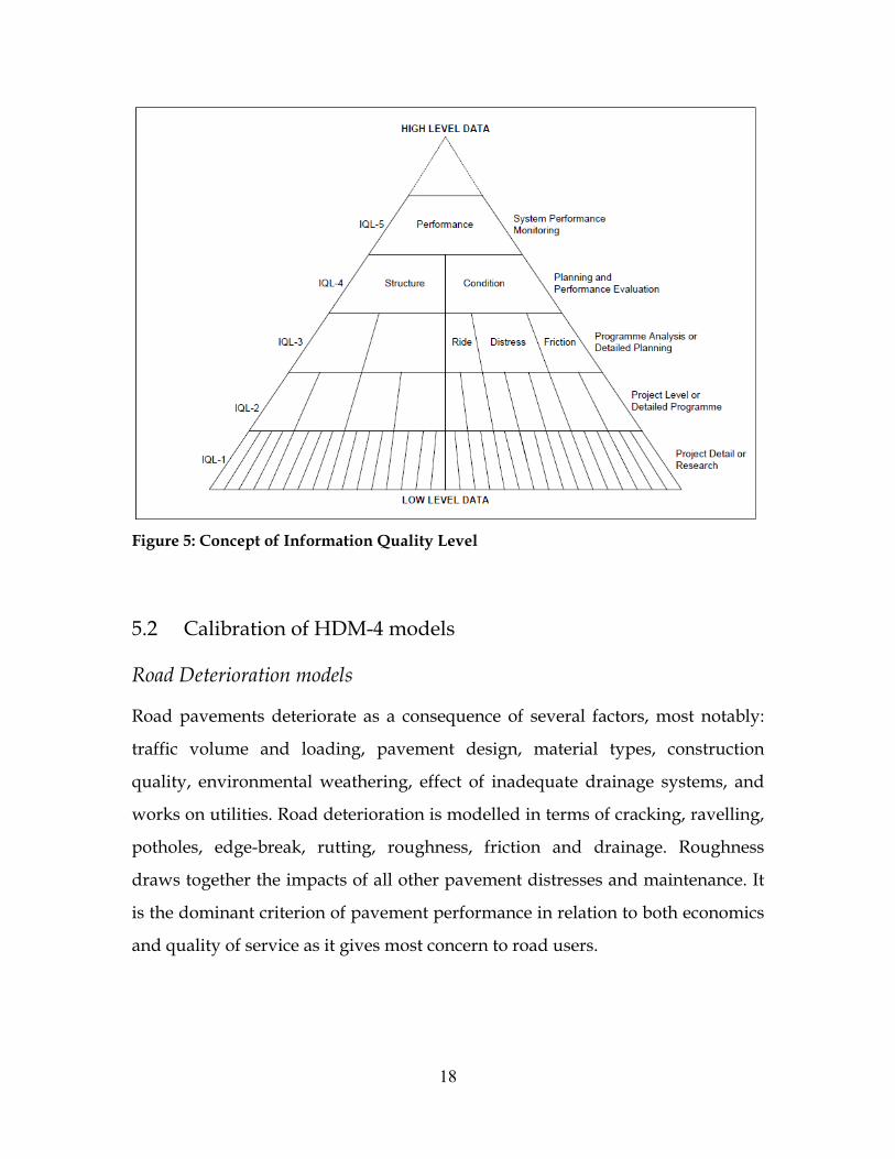
Road Network Aggregate Data

The entails defining relationships between high level aggregate data and low

level detailed data using the concept of Information Quality Level (IQL),

Paterson and Sculllion (1990). The IQL concept, depicted in Figure 5, allows data

to be structured in ways that suit the needs of different levels of decision making

and the variety of effort and sophistication of methods for collecting and

processing data.

Configuration of aggregate data will involve the definition of aggregate

information for the following: Traffic levels: e.g., low, medium, high; Geometry

class: in terms of parameters reflecting horizontal and vertical alignment;

Pavement characteristics: structure and strength parameters defined according to

pavement surface class; Road condition: ride quality, surface distress and surface

texture; and Pavement history: mainly construction quality and pavement age.

18

Figure 5: Concept of Information Quality Level

5.2 Calibration of HDM-4 models

Road Deterioration models

Road pavements deteriorate as a consequence of several factors, most notably:

traffic volume and loading, pavement design, material types, construction

quality, environmental weathering, effect of inadequate drainage systems, and

works on utilities. Road deterioration is modelled in terms of cracking, ravelling,

potholes, edge-break, rutting, roughness, friction and drainage. Roughness

draws together the impacts of all other pavement distresses and maintenance. It

is the dominant criterion of pavement performance in relation to both economics

and quality of service as it gives most concern to road users.

19

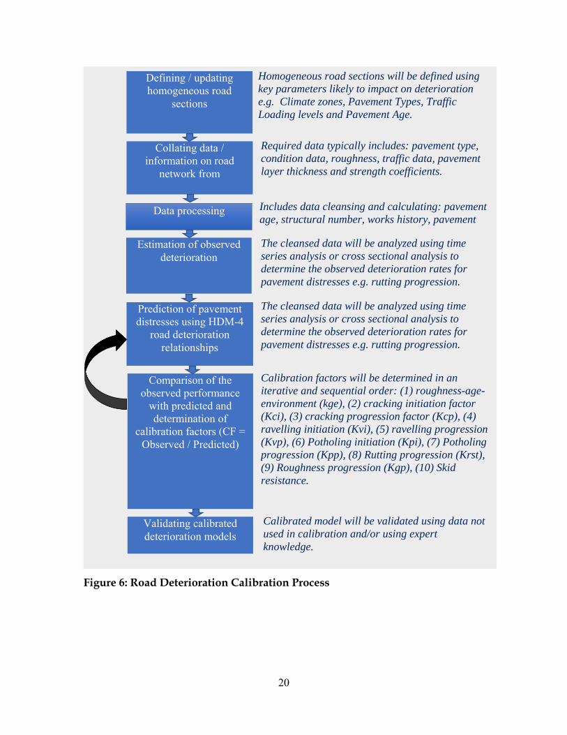
For each pavement type and each distress type there is a generic model which

describes how the pavement deteriorates. The approach for calibrating RD

models can be summarised by the steps illustrated by Figure 6.

Work Effects model, Standards and Unit Costs

The approach to calibrate Work Effects models will ensure the effects of works

performed on bituminous, unsealed and concrete roads are determined. We will

review maintenance history data and for various treatment types, determine the

condition of the road pavement before and after treatment. This information will

be used to calibrate HDM-4 works effects models for different types of

treatments such as new construction or reconstruction, overlay, and reseal

amongst others. When a works activity is performed, the immediate effects on

road characteristics and road use need to be specified in terms of the following:

pavement strength, pavement condition, pavement history, road use patterns,

and asset value.

The standard of road construction is dependent on the materials, degree of

compliance with design specifications, construction tolerances and the level of

site supervision. The key construction defect indicators in HDM-4 are:

Construction defect indicator for surfacing (CDS), which influences the

initiation of cracking and ravelling, and rutting due to plastic deformation

Construction defect indicator for the road-base (CDB), which influences

the formation of potholes

Relative compaction of the whole pavement (COMP), which affects

rutting.

It is important to define these construction defect indicators to depict the general

situation in Kenya.

20

Figure 6: Road Deterioration Calibration Process

Defining / updating homogeneous road

sections

Collating data / information on road

network from

Data processing

Estimation of observed deterioration

Prediction of pavement distresses using HDM-4

road deterioration relationships

Comparison of the observed performance

with predicted and determination of

calibration factors (CF = Observed / Predicted)

Validating calibrated deterioration models

Homogeneous road sections will be defined using key parameters likely to impact on deterioration e.g. Climate zones, Pavement Types, Traffic Loading levels and Pavement Age.

Required data typically includes: pavement type, condition data, roughness, traffic data, pavement layer thickness and strength coefficients.

Includes data cleansing and calculating: pavement age, structural number, works history, pavement

The cleansed data will be analyzed using time series analysis or cross sectional analysis to determine the observed deterioration rates for pavement distresses e.g. rutting progression.

The cleansed data will be analyzed using time series analysis or cross sectional analysis to determine the observed deterioration rates for pavement distresses e.g. rutting progression.

Calibration factors will be determined in an iterative and sequential order: (1) roughness-age-environment (kge), (2) cracking initiation factor (Kci), (3) cracking progression factor (Kcp), (4) ravelling initiation (Kvi), (5) ravelling progression (Kvp), (6) Potholing initiation (Kpi), (7) Potholing progression (Kpp), (8) Rutting progression (Krst), (9) Roughness progression (Kgp), (10) Skid resistance.

Calibrated model will be validated using data not used in calibration and/or using expert knowledge.

21

Standards refer to the levels of conditions and response that a road

administration aims to achieve in relation to functional characteristics of the road

network system. The choice of an appropriate standard is based on the road

surface class, the characteristics of traffic on the road section, and the general

operational practice in the study area based upon engineering, economic and

environmental considerations. In HDM-4, a standard is defined by a set of works

activities with definite intervention criteria to determine when to carry them out.

In general terms, intervention levels define the minimum level of service that is

allowed. Road agency resource needs for road maintenance are expressed in

terms of the physical quantities and the monetary costs of works to be

undertaken. The annual costs to road agency incurred in the implementation of

road works are calculated in economic and/or financial terms depending on the

type of analysis being performed. The cost of each works activity need to be

updated regularly and considered under the corresponding user-specified

budget category (capital, recurrent or special).

Road User Effects (RUE)

The impacts of the road condition, road design standards, and traffic levels on

road users are measured in terms of road user costs, and other social and

environmental effects. Road user costs comprise vehicle operation costs, costs of

travel time, and costs to the economy of road accidents. Vehicle operating costs

are obtained by multiplying the various resource quantities by the unit costs or

prices. Thus, the annual road user costs (RUC) are calculated for each vehicle

type, for each traffic flow period and for each road section alternative. HDM-4

RUE models have been calibrated to conditions in Kenya in a study conducted in

2011. Unit costs of various vehicle resource consumption will be collected in a

field survey and used to update the Kenya HDM-4 workspace.

22

5.3 Vehicle Fleet Data

Equivalent Standard Axle Load Factors (ESALF)

Axle load data from all weighbridges in Kenya will be used to derive equivalent

standard axle load factors for the representative vehicles included in Kenya

HDM-4 workspace. The approach to the task can be summarized as follows:

1. Review the axle configuration of the representative vehicles used in the

current HDM-4 workspace with data from weighbridges and from other

sources within Kenya and update if necessary;

2. Analyse the axle load data from weighbridges to establish the severity of

overloading particularly on strategic routes used by heavy vehicles and to

determine ESALF by vehicle type and region (defined by weighbridge

location);

3. Enter the calculated ESALF in HDM-4 workspace for Kenya.

Non-Motorized Transport

Relevant non-motorized transport modes need to be identified and defined in

Kenya HDM-4 workspace. It is expected that bicycles, pedestrians and animal

carts will be included as NMT modes in the Vehicle Fleet in HDM-4 workspace.

Traffic Growth

As a guide it will good to include traffic growth rates in the Vehicle Fleet. Ideally,

growth rates would be inferred from historical records of vehicle–km for traffic

in the project corridor. When such records do not exist, however, inferences have

to be drawn from: traffic counts; numbers of registered vehicles; fuel sales; GDP

growth; GDP per capita and population growth.

23

5.4 Updated Customized HDM-4 Workspace for Kenya

The outputs from the configuration and calibration tasks described in previous

sections will be used to produce an updated customized HDM-4 workspace for

analysing road investment choices in Kenya. The customized workspace will

contain vehicle fleet characteristics and resource consumption unit costs; traffic

growth rates; default unit costs of road works in financial and economic terms;

maintenance standards; asset valuation parameters; configuration datasets;

model calibration parameters; project analysis case studies; programme analysis

case study; and strategy analysis case study.

6 Challenges

The main challenges being encountered in the exercise to configure and calibrate

HDM-4 to conditions in Kenya relate to data. Some of the major challenges are

presented as follows:

1. Road agencies have been collecting and maintaining data for its road

network for some years. This data is being stored in various formats in the

agencies’ respective databases. It has been particularly difficult not only to

retrieve this data from the databases but also to obtain complete historical

data sets that can be used to calibrate HDM-4 RD and WE models.

2. Data on the current status of the road network is required in order to

configure and calibrate HDM-4 models. This data need to be collected

from the field however it is costly and time consuming.

3. A lot of field data is being collected and the processing of this data into

suitable formats required as inputs for carrying out HDM-4 configuration

and calibration poses a major challenge to the road agencies.

4. Dealing with the issue of missing incomplete or lack of data is also a major

challenge being encountered. This is being addressed by applying the IQL

concept and using look-up tables of representative road sections.

24

7 Conclusions

The case study presented in this paper has demonstrated how HDM-4 can be

established as a comprehensive decision support tool for use by the road

agencies in Kenya. This would enable the road agencies to carry out medium to

long-term planning of development and maintenance expenditure and

investigate investment choices on Kenya roads. Prior to using HDM-4 in any

country, the system should be configured and the relevant prediction models

should be calibrated to reflect local conditions. The major challenges being

encountered relate to availability of complete data sets, in particular the lack of

appropriate time series data on road pavement performance and traffic, for the

calibration of road deterioration models.

HDM-4 can be used to determine the effects of various funding levels. Both the

strategy and programme analysis tools optimize investment options subject to

available budget to minimize total transport costs by considering the costs to the

road authority and road users. To that end, HDM-4 provides a good framework

for ensuring that funds for maintenance of roads are distributed equitably

amongst road authorities, and provide value for money for the taxpayer. From

the foregoing, it is clear that there is the need for Kenya to adopt one configured

and calibrated HDM-4 workspace in order to improve the accuracy of

investment modelling and guide investment decision making in the sector.

25

References

Bennett, C.R. and Paterson, W.D.O. (2000). A Guide to Calibration and

Adaptation – Volume 5. International Study of Highway Development and

Management Series, World Road Association (PIARC), PARIS. ISBN: 2-84060-

063-3

Kerali, H.G.R., McMullen, D. and Odoki, J.B. (2000). Applications Guide –

Volume 2. International Study of Highway Development and Management

Series, World Road Association (PIARC), PARIS. ISBN: 2-84060-060-9

Odoki, J.B. and Kerali, H.G.R. (2006). Analytical Framework and Model

Descriptions – Volume 4. International Study of Highway Development and

Management Series, World Road Association (PIARC), PARIS. ISBN: 2-84060-

062-5

Paterson, W.D.O. and Scullion, T. (1990). Information Systems for Road

Management: Draft Guidelines on System Design and Data Issues. World Bank

Technical Paper INU 77, Infrastructure and Urban Development Department,

The World Bank, Washington, D.C.

Paterson, W.D.O. (1987). Road Deterioration and Maintenance Effects, Models

for Planning and Management. A World Bank Publication, The John Hopkins

University Press, Baltimore and London.

TRL, (2005). Overseas Road Note 5. A guide to road project appraisal. The

Department for International Development, UK. ISBN: 0-9543339-6-9