Embed Size (px)
Citation preview

CASE STUDY OF A LONG-LIVED THUNDERSNOW EVENT
Abstract
On 23 March 1966, thundersnow was reported over a period of 9 hours (non-consecutive) at Eau Claire, Wisconsin. This event is unique, as it constitutes the longest period of thundersnow (known to these authors) at a single station from a surface observation dataset of 226 stations spanning the years 1961-1990. In this study, the characteristics of a long-lived snowstorm with lightning and thunder are examined. Using model output from a simulation by the Workstation Eta (WS-Eta), we determine that the thermodynamic characteristics of the thundersnow event do not change appreciably with the evolution of the cyclone in this case. For the duration of the event, Eau Claire is north-northeast of the surface cyclone, with ample moisture, and forcing for ascent via a trough of warm air aloft (trowal) feature that is present upstream at 0000 UTC and then coinciding with Eau Claire at 1200 UTC. Negative equivalent potential vorticity (EPV) and conditional symmetric instability (CSI) are present in early cross-section analysis. Yet, elevated convective (potential) instability fails to develop toward the end of the event. These conclusions are bolstered by a WS-Eta run that provides an excellent meso-β simulation of the storm, with output similar to the 48-hr precipitation field. This thundersnow event resulted largely from the prolonged existence of frontogenesis in the presence of weak symmetric stability northeast of a surface cyclone. Localized soundings also exhibit many of the characteristics found in wintertime thunderstorm cases. On the larger scale, this scenario was created and maintained by the presence of a trowal airstream over the Eau Claire, Wisconsin, region for an extended period.
Corresponding Author: Patrick Market, 302 ABNR, Columbia, MO 65211 or via e-mail:
Patrick S. Market, Rebecca L. Ebert-Cripe
Department of Soil, Environmental and Atmospheric SciencesUniversity of Missouri-Columbia
Columbia, Missouri
Michael BodnerDOC/NOAA/NWS/NCEP/Hydrometeorological Prediction Center
Camp Springs, Maryland

104 National Weather Digest
Market et al.
1. Introduction
On 23 March 1966, an extended period of thundersnow occurred at Eau Claire, Wisconsin. From 0300 UTC to 1200 UTC, 4 separate thundersnow observations were recorded at the surface weather station with a recurrence time of 2-3 hours. Locally, 18 cm (7 in) of snow fell at Eau Claire with locations in bands north of the city receiving as much as 45 cm (18 in) in storm-total snow fall. In fact, substantial snowfall totals occurred over parts of four states (Fig. 1) during 22-24 March 1966, and near blizzard conditions existed in some locations in the wake of the snowfall from this system. At least one other location (Sioux Falls, Iowa) reported thundersnow with this event, just prior to the onset of the Eau Claire event, and there may have been other observations during this storm that were never reported. The climatology of Branick (1997) suggests strongly that thundersnow events have historically been underrepresented. Yet, the event at Eau Claire had one of the longest known durations of observed thundersnow known to these authors. In an effort to understand better this heavy snowfall event as well as the environment that produced lightning, data from that time period were analyzed and also used to initialize a mesoscale numerical model. Output from a run of the Workstation Eta was examined in order to understand the mesoscale processes that shaped a thundering snowstorm in this system.
The purpose of this study is to reveal the characteristics of a particularly strong, long-lived thundersnow event, within which thundersnow existed over a period of nine non-consecutive hours. Clearly, some persistent process(es) acted to generate (and regenerate) the conditions necessary for lightning and thunder. Two objectives are identified to accomplish the aforementioned purpose. This research seeks to:
Determine if convection was slantwise or upright in •nature, or if the environment evolved from one type to the other. Examine the static stability and its tendency to determine •the thermodynamic environment that harbored recurrent lightning and thunder.
To complete our study, this paper takes the followingformat: section 2 addresses points of methodology, including
the objective analysis of observed upper air data as well as model architecture and its performance; section 3 provides a brief synoptic analysis of the event; section 4 features mesoscale analyses from the model output; in section 5 we offer some concluding remarks.
2. Methodology
This study relies on both observed data and a special run of the Workstation Eta (hereafter the WS-Eta) mesoscale numerical weather forecasting system developed at the National Center for Atmospheric Research (NCAR). The WS-Eta is based upon the operational Eta model (Black 1994) at the NOAA/National Weather Service (NWS) National Centers for Environmental Prediction (NCEP). In this section, we explore the observed data employed in this study, how it is analyzed objectively, and the architecture of the WS-Eta, from which more sophisticated diagnostics are derived.
a. Observed data Upper-air data from up to 82 North American radiosonde observation stations were used in this study. These radiosonde data were objectively analyzed (Barnes 1973) using the General Meteorological Package (GEMPAK) as discussed by Koch et al. (1983) in order to facilitate more
Figure 1: A map showing the 48-hour total snowfall accumulation (0000 UTC 22 March 1966to 0000 UTC 24 March 1966) in inches from cooperative climate observation stations. Contoursat 1, 5, 10, and 15 inches (2.5, 12.7, 25.4, and 38.1 cm). Eau Claire, Wisconsin, is denoted bya star.
27
Fig. 1. A map showing the 48-hour total snowfall accumulation (0000 UTC 22 March 1966 to 0000 UTC 24 March 1966) in inches from cooperative climate observation stations. Contours at 1, 5, 10, and 15 inches (2.5, 12.7, 25.4, and 38.1 cm). Eau Claire, Wisconsin, is denoted by a star.

Volume 31 Number 2 ~ December 2007 105
A Long-lived Thundersnow Event
advanced diagnostics such as Q vectors and frontogenesis from the uniform grid. The grid was centered on 39.8°N. and 99.5°W. using a polar stereographic projection situated over North America and possessing 32 points in the east-west direction and 25 points in the north-south direction. The horizontal grid-spacing was 150 km, with a vertical spacing of 50 mb, from 1000 to 300 mb, inclusive. Two passes were made through the data, and a search radius of 25 Δn (25 grid spaces) was used, as suggested by Koch et al. (1983). The spectral response function, γ, is a means to extract more signal from smaller waves; for these analyses, γ was set to 0.25. With these criteria, a wave of 12 Δn (1800 km when Δn=150km), is ~90% resolved, resulting in grids with sufficient resolution to generate a satisfactory synoptic analysis.
b. Numerical model simulation The WS-Eta simulation presented here used NCEP/NCAR Reanalysis Data (Kalnay et al. 1996) for initial and 6-hourly lateral boundary conditions. In this work, the WS-Eta possesses a horizontal grid spacing of 32 km (Fig. 2) and 45 vertical levels, with one-way, parasitic lateral boundary conditions. The latter condition only permits the introduction of waves from the outer grid on to the inner,
model domain, but waves that are generated on the model grid are not able to impact the boundary conditions; upscale feedback to the larger environment is thus not considered. This architecture was the same as used for operational WS-Eta runs at the NCEP Hydrometeorological Prediction Center (HPC) at the time the research was conducted. It allows for a hydrostatic rendering of the atmosphere on a scale that requires the parameterization of cumulus convection.
Physical parameterization schemes that are used
include the Mellor-Yamada (1982) planetary boundary layer scheme, and the Betts-Miller-Janjic (BMJ) cumulus parameterization scheme (Betts and Miller 1986; Janjic 1994). The BMJ scheme was chosen, as it responds to both a shallow and deep convective environment, and a recent internal HPC study suggested that the BMJ tended to perform better with QPF on the cold side of fronts. Four soil levels are incorporated into the model. Along the west-east axis, there are 54 mass grid points along the first row, and 83 rows in the north-south direction. For a 32 km horizontal grid-spacing, a time step of 90 seconds is used. The grid spacing in the east-west direction is therefore 0.222° and in the north-south direction 0.205°, with the top of the atmosphere set at 25 hPa. The specific model solution presented here was begun at 1200 UTC 22 March 1966 and run for 36 hours.
This model architecture was considered adequate for the task. Although use of a horizontal grid spacing of 32 km is relatively coarse even by current standards, the selected grid spacing allowed for useful solutions on the meso-β and lower meso-α scales. While this build will not allow the very finest precipitation bands to be resolved, the parent environment in which they form is well-rendered. In the absence of higher-resolution data from which to initialize, and radar or satellite imagery for even a subjective verification, results from a finer-scale model run, while of great curiosity, were considered less than ideal.
c. Model performanceThe comparison of the 36-hour accumulated liquid
equivalent precipitation field from the WS-Eta (Fig. 3) to the actual storm-total (48-hour) snow field (Fig. 1) for the study area both ending at 0000 UTC on 24 March 1966 reveals a workable subjective solution. Both analyses place a large mesoscale band of precipitation across lower Minnesota and northern Wisconsin southwestward into Iowa and Nebraska. Throughout this large mesoscale band, there are smaller, heavier observed bands of snow that developed (Fig. 1). The heaviest observed snowband that was produced during the event occurred on the eastern Minnesota-Wisconsin border where greater than 15 inches of snow fell.
On the WS-Eta 36-hour output (Fig. 3), this snowfall was captured as one large band and shown as a liquid equivalent of 2.25 inches snow-to-liquid. The ratio of predicted liquid to actual snow was nearly 7:1, which is a viable number in March when snowfall tends to be more moist and dense (Baxter 2003). In the Eau Claire area, a total of 7 inches was reported by observers and shown on the subjective analysis. The WS-Eta also showed that Eau Claire received between 1.5 and 1.75 inches of liquid equivalent precipitation. If the rainfall amount prior to the
Figure 2: The 32-km WS-Eta grid architecture for this run.
28
Fig. 2. The 32-km WS-Eta grid architecture for this run.

106 National Weather Digest
Market et al.
Fig. 4. Meteorogram for Eau Claire, Wisconsin, for the period 0000 UTC to 1500 UTC on 23 March 1966. The top bar depicts the temperature (solid) and dew point (dashed) trends (°F); the second is a barograph of sea level pressure (mb); the middle bar shows the wind speed trend (solid line; knots) while the shafts with barbs show the wind direction and speed, respectively, as one might see in a standard station model; the fourth bar depicts the visibility trend (statute miles); the bottom bar shows standard symbols for weather type (above) and sky condition (below).
Figure 4: Meteorogram for Eau Claire, Wisconsin, for the period 0000 UTC to 1500 UTC on 23March 1966. The top bar depicts the temperature (solid) and dew point (dashed) trends (◦F ); thesecond is a barograph of sea level pressure (mb); the middle bar shows the wind speed trend (solidline; knots) while the shafts with barbs show the wind direction and speed, respectively, as onemight see in a standard station model; the fourth bar depicts the visibility trend (statute miles);the bottom bar shows standard symbols for weather type (above) and sky condition (below).
30
onset of measurable snow is taken into account, then this is a valid analysis of the WS-Eta output of total accumulated precipitation. It can be stated that the total accumulated precipitation output by the WS-Eta captured the mesoscale banding that took place and the location where those bands formed, if not the fine-scale structures found in the observed snow swath. We note, however, that the eastern half of the modeled precipitation field (Fig. 3) tends to align about 100 km south of the observed precipitation field. This is an important point that will be revisited in our later discussions of instability and lightning generation. Nevertheless, these results represent the best match to the observations that we were able to obtain.
Thunder, lightning, and heavy snowfall were observed in the Eau Claire area, so it is fair to state that convection did take place. Yet, it is important to note that while the precipitation scheme activated for this event, no convective precipitation was rendered by the WS-Eta. This suggests that perhaps convection induced by upright and symmetric instability was limited by the model, or the use of a global initialization contributed to both limitations in the deployment of the convective scheme as well as the noted spatial QPF errors. Indeed, a model with a grid spacing of 32 km, which
0.25
0.25
0.25
0.25
0.250.25
0.25
0.25
0.25
0.5
0.5
0.5
0.50.5
0.5
0.75
0.75
0.75
0.750.75
0.750.75
1
1
1
1.251.51.75
22.25
0 1 2
EAU
Figure 3: The WS-Eta accumulated liquid precipitation forecast (solid, every 0.25” (6.35 mm));shaded over 1.0” (25.4 mm) for the 36-hour period from 1200 UTC 22 March 1966 to 0000 UTC24 March 1966. Eau Claire, Wisconsin, is marked by the letters EAU.
29
Fig. 3. The WS-Eta accumulated liquid equivalent precipitation forecast (solid, every 0.25” (6.35 mm)); shaded over 1.0” (25.4 mm) for the 36-hour period from 1200 UTC 22 March 1966 to 0000 UTC 24 March 1966. Eau Claire, Wisconsin, is marked by the letters EAU.
is parameterizing convection over a large area, is unlikely to account for isolated convective episodes, especially when relatively small amounts of instability are present, and tend to be elevated, such as in cold season cyclones.
3. Synoptic Analysis
First, we shall focus our attention on the observed data from a 12-hour period that encompassed the most significant weather at Eau Claire, Wisconsin. From 0300 UTC to 1200 UTC on 23 March 1966, snow with thunder was reported at Eau Claire for 9 non-consecutive hours, as shown by the meteorogram for the period 0000 UTC 23 March 1966 through 1500 UTC 23 March 1966 (Fig. 4). Although the accumulated snowfall totaled only 18.5 cm (7.3 inches), at Eau Claire during a period of ~ 27 hours, the long-lived nature of lightning and thunder with this event demands further scrutiny. In the evaluation of this case, the 48-hour snowfall accumulation has been calculated and presented in Fig. 1. Notice the presence of a large band of snow from northern Wisconsin to western Iowa; within this large band, there are smaller mesoscale bands embedded causing a snow gradient to be distinctly identified.

Volume 31 Number 2 ~ December 2007 107
A Long-lived Thundersnow Event
The time period for which actual data are analyzed in this case study is 0000 UTC 23 March 1966. This is three hours before the first report of thundersnow was issued by human observers at the Eau Claire Municipal Airport. Examination of the surface analysis from 0000 UTC 23 March 1966 (Fig. 5) reveals a deepening cyclone southwest of Eau Claire,
Fig. 6. Analysis of the 850-mb geopotential height (solid; every 30 gpm) and temperature (dashed; every 5°C) valid at 0000 UTC 23 March 1966.
−25
−20
−15
−10
−5
0
5
10
10
15
20
660323/0000 850 MB TMPC
1350
1350
1380
1380
1410
1410
1440
1440
1470
1470
1470
1500
1500
1500
1500
1530
1530
1530
1560
660323/0000 850 MB HGHT
Figure 6: Analysis of the 850-mb geopotential height (solid; every 30 gpm) and temperature(dashed; every 5◦C) valid at 0000 UTC 23 March 1966.
32
Wisconsin, thereby placing the thundersnow northeast of the surface cyclone center. A warm front extends from northwestern Missouri through northern Indiana, putting Eau Claire north of the warm frontal boundary. A weak inverted trough extends to the northeast of the cyclone center, a region with temperatures cooler than at Eau Claire,
but also several surface reports of thunderstorms, indicating elevated convective activity at the time.
The 850-mb height and isotherm analysis for 0000 UTC 23 March 1966 (Fig. 6), shows warm advection (WAA) just south of the Eau Claire area, in a wide band that covers eastern Iowa, northern Illinois, and western Michigan. WAA just south of the event location signifies where the warm conveyor belt (WCB) is ascending into the upper Midwest around the cyclonic curvature of the upper-level low.
The 500 mb heights and vorticity map (Fig. 7) reveal the presence of two troughs. The first located over Missouri, while a relatively weak negatively-tilted trough, did significantly affect this particular event, as will be explained shortly. The second, deeper trough is positively tilted, and located through portions of Kansas, the panhandle of Oklahoma and Texas and into
Fig. 7. Analysis of the 500-mb geopotential height (solid; every 60 gpm) and absolute vorticity (dashed, every 2 x 10⁻⁵ s-1; vorticity maxima are denoted by ‘X’ while minima are marked with ‘N’) valid at 0000 UTC 23 March 1966.
5280
5340
5400
54605520
55805640
5700
660323/0000 500 MB HGHT
46 6
6
6
6
6
6
8
8
8
10
10
10
10
12
12
12
12
12
14
14
14
16
16
18
18 20
X
X
X
X
N
N
N
N
N
660323/0000 500 MB AVORWND (*10**5)
Figure 7: Analysis of the 500-mb geopotential height (solid; every 60 gpm) and absolute vorticity(dashed; every 2 × 10⁻⁵s−1) valid at 0000 UTC 23 March 1966.
33
Fig. 5. The surface analysis valid at 0000 UTC 23 March 1966. Sea level pressure (solid; every 4 mb) and temperature (dashed; every 10°F) are analyzed subjectively. Eau Claire is identified by the flying arrow at upper right.

108 National Weather Digest
Market et al.
Fig. 8. Analysis of 300-mb geopotential height (every 120 gpm) and isotachs (dashed; every 10 kts starting at 50 kts) for 0000 UTC 23 March 1966. The location of Eau Claire, Wisconsin, is marked with an ‘X’.
Fig. 10. Analysis of the 400-700 mb layer mean Q-vector and its divergence (positive is solid, negative is dashed; every 10 x 10-14 mb m-2 s-1) at 0000 UTC 23 March 1966. The location of Eau Claire, Wisconsin, is marked with an ‘X’.
Fig. 9. Analysis of the 900-700-mb mean relative humidity (every 10%; dashed below 50%), a linear average of 900, 800, and 700-mb relative humidities at 0000 UTC 23 March 1966. The location of Eau Claire, Wisconsin, is marked with an ‘X’.
jet structure. Indeed, at 300 mb the Eau Claire region was home to the center of a local divergence maximum in excess of 3 x 10⁻⁵ s-1 (not shown).
The analysis of 900-700-mb mean layer relative humidity (Fig. 9), shows an area where the mean layer relative humidity is 70% or greater. Sufficient moisture is present throughout the lower- to mid-troposphere for the production of precipitation. This map shows that not only Eau Claire, but the entire area along and north of the warm frontal boundary, possessed significant moisture.
Figure 10 is the analysis of 400-700-mb layer Q-vector divergence. Q-vectors describe the changes that a parcel’s potential temperature gradient vector undergoes as the parcel moves with the geostrophic wind. Here, we employ the layer Q-vector which, based upon the GEMPAK code, we write here in a simplified form as
(1)
where gV
is the geostrophic wind, and θ is the potential temperature. The divergence of this vector is then formed simply as Q
•∇ , resulting in units of mb m-2 s-1. With this
formulation, when the Q-vector divergence is negative, then forcing for upward vertical motion would result and Q-vector fields appear to converge. At 0000 UTC there is strong Q-vector convergence to the southwest of Eau Claire; this region extends later to include Eau Claire by 1200 UTC, although the maximum at that time still resides southwest
∇•
∂∂
+
∇•
∂∂
∂∂
= jy
Vi
xVpQ gg
layerˆˆ θθ
θ
New Mexico. This configuration suggests a system that will continue to deepen as it translates. Indeed, the trough location evinces a favorable baroclinic structure.
The analysis at 300-mb (Fig. 8) indicates a meridional trough through western Kansas, the panhandle of Oklahoma and into western Texas. This is in association with a curved 80-kt jet streak. Eau Claire is located in the left exit region of this curved jet on the poleward side. This is typically an area of enhanced upward motion and convergence (Moore and Van Knowe 1992), which is verified shortly in the 400-700 mb Q-vector analysis. There is also evidence of a coupled
660323/0000 280 K VECSUBWSUBV
700
750800
850
850
850 900
660323/0000 280 K PRES
Figure 11: An analysis of the 280 K isentropic surface with pressure (bold solid; every 50 mb) and
storm-relative streamlines (where �C has components of u = +10.9 m s−1, v = + 6.4 m s−1),validat 0000 UTC 23 March 1966. Analysis does not fill the entire map, because the isentropic surfaceintersects the earth’s surface. Bold arrow denotes axis of cold conveyor belt.
37

Volume 31 Number 2 ~ December 2007 109
A Long-lived Thundersnow Event
of the city. This suggests significant forcing for upward motion in association with the surface cyclone. With the presence of synoptic-scale upward motion, and ample moisture in the layer, the ingredients needed for significant snow are becoming assembled.
Isentropic surfaces are also used in order to diagnose storm-relative ( CV
− ) airstream structures and their
associated descending and ascending motions, visualized as conveyor belts (e.g., Carlson 1991); here V
is the actual
wind, and C
is the storm motion. The first surface that was analyzed was the 280 K isentropic surface (Fig. 11) at 0000 UTC 23 March 1966. On this surface the range in pressure height is from 900 mb through 700 mb. The streamlines on this surface denote where the cold conveyor belt (CCB) is descending from higher levels toward the ground, and beginning to swirl around the backside of the surface low pressure, before intersecting the surface. The 296 K isentropic surface (Fig. 12) from 0000 UTC 23 March 1966, reveals pressures from 950-400 mb. The warm conveyor belt (WCB) is apparent as warm air from the lower Ohio River Valley is being pulled up and around the surface low. Starting from the 950-mb level, warm air is ascending and wrapping around the surface low to a level of 550 mb. This image is a good representation of the vertical structure surrounding a cyclonic system on an isentropic surface. Finally, on the 312 K isentropic surface (Fig. 13) the levels
Fig. 11. An analysis of the 280 K isentropic surface with pressure (bold solid; every 50 mb) and storm-relative streamlines (where has components of u= +10.9 m s-1, v= + 6.4 m s-1), valid at 0000 UTC 23 March 1966. Analysis does not fill the entire map, because the isentropic surface intersects the earth’s surface. Bold arrow denotes axis of cold conveyor belt.
660323/0000 280 K VECSUBWSUBV
700
750800
850
850
850 900
660323/0000 280 K PRES
Figure 11: An analysis of the 280 K isentropic surface with pressure (bold solid; every 50 mb) and
storm-relative streamlines (where �C has components of u = +10.9 m s−1, v = + 6.4 m s−1),validat 0000 UTC 23 March 1966. Analysis does not fill the entire map, because the isentropic surfaceintersects the earth’s surface. Bold arrow denotes axis of cold conveyor belt.
37
660323/0000 296 K VECSUBWSUBV
400
450
500 550 600 650
650
700
750
800
800
850
900
950
660323/0000 296 K PRES
Figure 12: An analysis of the 296 K isentropic surface with pressure (bold solid; every 50 mb)
and storm-relative streamlines (where �C has components of u = +10.9 m s−1, v = + 6.4 ms −1), valid at 0000 UTC 23 March 1966. Analysis does not fill the entire map, because theisentropic surface intersects the earth’s surface. Bold arrow denotes axis of warm conveyor belt.
38
Fig. 12. An analysis of the 296 K isentropic surface with pressure (bold solid; every 50 mb) and storm-relative streamlines (where has components of u = +10.9 m s-1, v = + 6.4 m s-1), valid at 0000 UTC 23 March 1966. Analysis does not fill the entire map, because the isentropic surface intersects the earth’s surface. Bold arrow denotes axis of warm conveyor belt.
Fig. 13. An analysis of the 312 K isentropic surface with pressure (bold solid; every 50 mb) and storm-relative streamlines (where has components of u = +10.9 m s-1, v = + 6.4 m s-1), valid at 0000 UTC 23 March 1966. Bold arrow denotes axis of dry conveyor belt. The location of Eau Claire, Wisconsin, is marked with an ‘X’.
C
C
C

110 National Weather Digest
Market et al.
Fig. 14. A skew-T log p analysis for Eau Claire, Wisconsin (KEAU), valid at 0000 UTC 23 March 1966, from the 12-hour forecast fields produced by the WS-Eta. Inset of “Theta-E vs Height” features θe as the x-axis variable, marked arbitrarily every 10K; pressure appears as the y-axis variable, ticked every 100 mb from 1000 mb to 500 mb, and marked at 800, 700, and 600 mb.
800
600
700
KEAU 19660323/0000V012
Figure 14: A skew-T log p analysis for Eau Claire, Wisconsin (KEAU), valid at 0000 UTC 23March 1966, from the 12-hour forecast fields produced by the WS-Eta. Inset of “Theta-E vsHeight” features θe as the x-axis variable, marked arbitrarily every 10K; pressure appears as they-axis variable, marked every 100 mb from 1000 mb to 500 mb.
40
start at 600 mb and continue to 300 mb. This image gives a representation of the dry descending airstream penetrating toward the surface over the southern plains, wrapping into the cyclone and providing contrast with the warm moist air on lower surfaces that are being advected and lifted into the cyclone. Yet, there is ascent diagnosed at this time over Eau Claire. While unsaturated, the air (as deduced from soundings, discussed shortly) is not terribly dry, and the cooling from ascent in this flow only serves to drive up the relative humidity. While not in strict conformance with Nicosia and Grumm (1998) for the production of negative equivalent potential vorticity, this situation certainly supports the production of precipitation.
4. Mesoscale Analysis
Having established the synoptic setting that supported this event using actual data, we turn now to the mesoscale environment as rendered by the WS-Eta. In this section, the output generated by the WS-Eta provides insight into the dynamics that contributed to the duration and magnitude of this snowfall event.
a. Assessing static stabilityWe now examine the model
solutions to assess the static stability and its tendency at Eau Claire, Wisconsin, between 0000 UTC and 1200 UTC 23 March 1966. We will begin with an examination of the modeled thermodynamic profiles and finish with calculations of static stability tendency (Bluestein 1992) for the crucial layer in the storm.
We begin our analysis with the 12 hour forecast (Fig. 14) valid at 0000 UTC 23 March 1966. Although quite moist through a significant depth, this sounding is also moist statically stable throughout the troposphere. The 700-500 mb lapse rate is 5.1°C km-1. Note also the veering wind profile through the troposphere, maximized in the 2-5 km layer. This warm air advection signature is critical for destabilizing the environment over Eau Claire, Wisconsin, over the ensuing 12 hours. Of course, this sounding also shows a surface based layer nearly 1 km deep that is above freezing. This matches quite closely the actual surface observation at Eau Claire at 0000 UTC (Figs. 4 and 5).
By 0300 UTC (Fig. 15), the surface based above freezing layer is more shallow and cold enough to support
Fig. 15. A skew-T log p analysis for Eau Claire, Wisconsin (KEAU), as in Fig. 14 but valid at 0300 UTC 23 March 1966, from the 15-hour forecast fields produced by the WS-Eta. Inset axes as in Fig. 14.
KEAU 19660323/0300V015
Figure 15: A skew-T log p analysis for Eau Claire, Wisconsin (KEAU), as in Fig. 14 but valid at0300 UTC 23 March 1966, from the 15-hour forecast fields produced by the WS-Eta.
41
Volume 31 Number 2 ~ December 2007 111
A Long-lived Thundersnow Event
KEAU 19660323/0600V018
Figure 16: A skew-T log p analysis for Eau Claire, Wisconsin (KEAU), as in Fig. 14 but valid at0600 UTC 23 March 1966, from the 18-hour forecast fields produced by the WS-Eta.
42
Fig. 16. A skew-T log p analysis for Eau Claire, Wisconsin (KEAU), as in Fig. 14 but valid at 0600 UTC 23 March 1966, from the 18-hour forecast fields produced by the WS-Eta. Inset axes as in Fig. 14.
KEAU 19660323/0900V021
Figure 17: A skew-T log p analysis for Eau Claire, Wisconsin (KEAU), as in Fig. 14 but valid at0900 UTC 23 March 1966, from the 21-hour forecast fields produced by the WS-Eta.
43
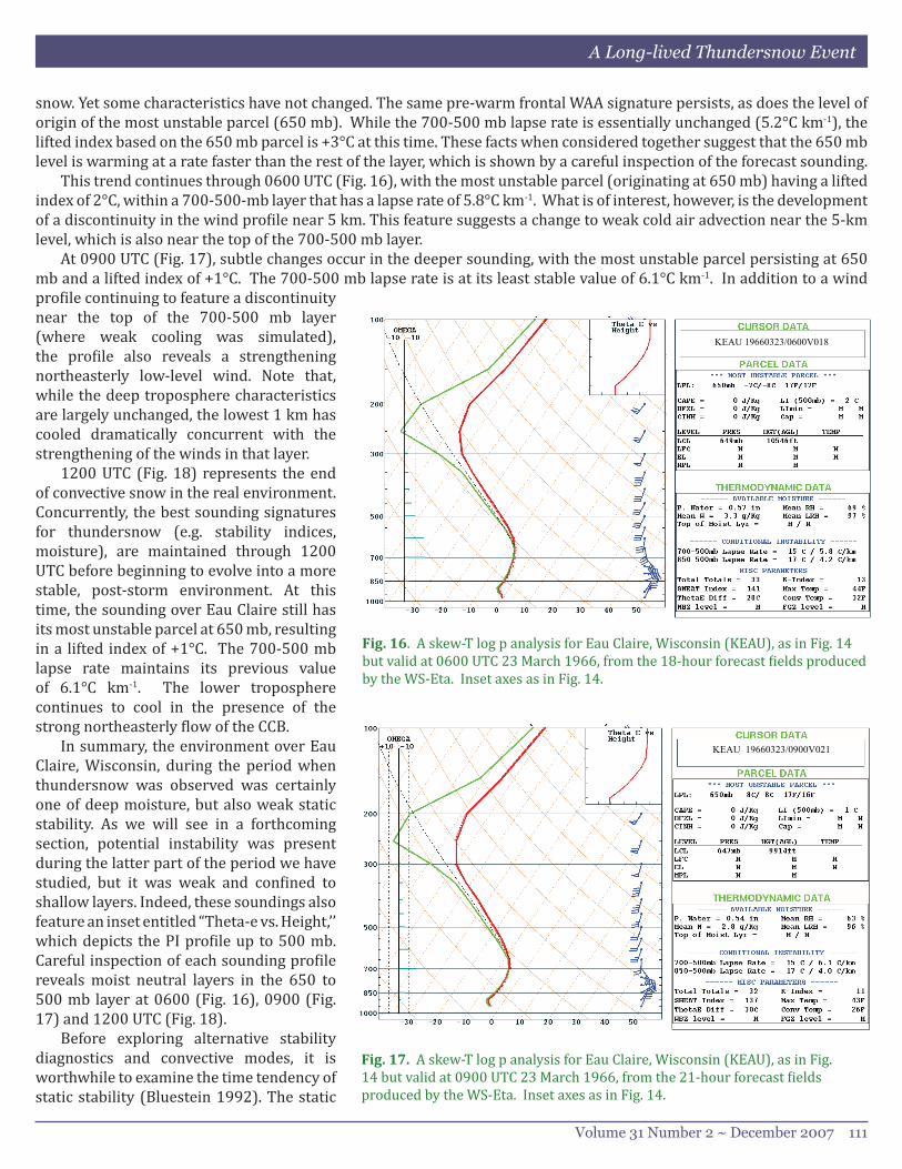
Fig. 17. A skew-T log p analysis for Eau Claire, Wisconsin (KEAU), as in Fig. 14 but valid at 0900 UTC 23 March 1966, from the 21-hour forecast fields produced by the WS-Eta. Inset axes as in Fig. 14.
snow. Yet some characteristics have not changed. The same pre-warm frontal WAA signature persists, as does the level of origin of the most unstable parcel (650 mb). While the 700-500 mb lapse rate is essentially unchanged (5.2°C km-1), the lifted index based on the 650 mb parcel is +3°C at this time. These facts when considered together suggest that the 650 mb level is warming at a rate faster than the rest of the layer, which is shown by a careful inspection of the forecast sounding.
This trend continues through 0600 UTC (Fig. 16), with the most unstable parcel (originating at 650 mb) having a lifted index of 2°C, within a 700-500-mb layer that has a lapse rate of 5.8°C km-1. What is of interest, however, is the development of a discontinuity in the wind profile near 5 km. This feature suggests a change to weak cold air advection near the 5-km level, which is also near the top of the 700-500 mb layer.
At 0900 UTC (Fig. 17), subtle changes occur in the deeper sounding, with the most unstable parcel persisting at 650 mb and a lifted index of +1°C. The 700-500 mb lapse rate is at its least stable value of 6.1°C km-1. In addition to a wind profile continuing to feature a discontinuity near the top of the 700-500 mb layer (where weak cooling was simulated), the profile also reveals a strengthening northeasterly low-level wind. Note that, while the deep troposphere characteristics are largely unchanged, the lowest 1 km has cooled dramatically concurrent with the strengthening of the winds in that layer.
1200 UTC (Fig. 18) represents the end of convective snow in the real environment. Concurrently, the best sounding signatures for thundersnow (e.g. stability indices, moisture), are maintained through 1200 UTC before beginning to evolve into a more stable, post-storm environment. At this time, the sounding over Eau Claire still has its most unstable parcel at 650 mb, resulting in a lifted index of +1°C. The 700-500 mb lapse rate maintains its previous value of 6.1°C km-1. The lower troposphere continues to cool in the presence of the strong northeasterly flow of the CCB.
In summary, the environment over Eau Claire, Wisconsin, during the period when thundersnow was observed was certainly one of deep moisture, but also weak static stability. As we will see in a forthcoming section, potential instability was present during the latter part of the period we have studied, but it was weak and confined to shallow layers. Indeed, these soundings also feature an inset entitled “Theta-e vs. Height,’’ which depicts the PI profile up to 500 mb. Careful inspection of each sounding profile reveals moist neutral layers in the 650 to 500 mb layer at 0600 (Fig. 16), 0900 (Fig. 17) and 1200 UTC (Fig. 18).
Before exploring alternative stability diagnostics and convective modes, it is worthwhile to examine the time tendency of static stability (Bluestein 1992). The static

112 National Weather Digest
Market et al.
stability tendency equation:
(2)
represents the local changes in static stability due to changes in four different terms: differential temperature advection (first term on the right-hand side), vertical advection of static stability (second term on the right-hand side), vertical stretching or shrinking of an air column (third on the right-hand side), and differential diabatic heating (fourth on right-hand side). When the differential temperature advection term is considered, then it can be assumed that it is equivalent to geostrophic stability advection and differential ageostrophic temperature advection. In a quasigeostrophic atmosphere, ageostrophic temperature advection is neglected, and hence only geostrophic stability is considered (Bluestein 1992). We note that the geostrophic stability advection can only transport stability from one place to another. It can neither create nor destroy stability. Thus, the ageostrophic wind is crucial in this term for affecting changes in stability. Also, the process of vertical advection cannot create or destroy stability. Static stability can be created or destroyed locally through
KEAU 19660323/1200V024
Figure 18: A skew-T log p analysis for Eau Claire, Wisconsin (KEAU), as in Fig. 14 but valid at1200 UTC 23 March 1966, from the 24-hour forecast fields produced by the WS-Eta.
44
Fig. 18. A skew-T log p analysis for Eau Claire, Wisconsin (KEAU), as in Fig. 14 but valid at 1200 UTC 23 March 1966, from the 24-hour forecast fields produced by the WS-Eta. Inset axes as in Fig. 14.
0.0
0.0 3.0 6.0 9.0
Time (UTC)12.0 15.0
-1.5x10⁻⁶
-1.0x10⁻⁶
5.0x10⁻⁷
1.0x10⁻⁶
1.5x10⁻⁶
-5.0x10⁻⁷
K m
b-1 s
-1
Figure 19: A plot from the WS-Eta output of the static stability tendency (K mb−1s−1) versustime for the period 0000 UTC to 1200 UTC, for the layer 700-600 mb over Eau Claire, WI.
45
Fig. 19. An analysis plot from the WS-Eta output of the static stability tendency (K mb-1 s-1) versus time for the period 0000 UTC to 1200 UTC, for the layer 700-600 mb over Eau Claire, WI.
the stretching or shrinking of an air column or through differential diabatic heating (Bluestein 1992).
In this study, each term is calculated for the 700-600 mb layer using a 6-hr centered, time difference. This approach places the bottom of the layer in question at or near the top of the frontal inversion. All of the terms come from the output fields except for the last (differential diabatic heating) term, which is solved for as a residual. Perturbation analysis of the kind used by Moore (1985) revealed that error accounts for no more than 5% of the differential diabatic heating term.
A plot of the static stability tendency (Fig. 19) shows a marked trend toward destabilization in the model over Eau Claire, WI, beginning after 0300 UTC and lasting until after 0900 UTC. Assessing the static stability tendency equation at 650 mb over Eau Claire, we see that the vertical advection of stability was negligible throughout the period, while the differential temperature advection and stability divergence terms tend to offset one another (Fig. 20). Yet differential temperature advection was the dominant of the three terms. Indeed, a careful examination of the model sounding at 0600 and 0900 UTC reveals no change in the temperature at 700 mb, but several degrees of cooling at 600 mb.
The differential diabatic heating term (Fig. 21) contributed consistently to stabilization during the crucial period. This behavior indicates an increase in diabatic heating with height, which is due, in part, to the moister environment at the bottom of the layer (700 mb) than the top (600 mb). Yet, even within the confines of the established uncertainty, the differential advection of θ dominated over Eau Claire in this case. That the differential diabatic heating and differential temperature advection terms both should be minimized at 0900 UTC is consistent with the presence of the trowal (trough of warm air aloft) axis over EAU at that time. The trowal is a canyon of warm moist air that often parallels the surface occluded front, wraps cyclonically around the poleward side of an extratropical cyclone (e.g., Moore et al. 2005), and is often associated with a westward
dtdQ
TcppppV
ppt pp

Volume 31 Number 2 ~ December 2007 113
A Long-lived Thundersnow Event
extension of the warm conveyor belt (Carlson 1991) known as the “trowal airstream’’ (Martin 1999).
In all, this exercise shows more clearly the various processes that lead to destabilization. The decrease with height of warm air advection and the increase with height of diabatic heating, both above the top of the inversion, strongly suggest the presence of the trowal while paving the way for more elaborate stability analyses.
b. Assessing symmetric stabilityPetterssen (1956) defined frontogenesis as the tendency
toward the formation of a discontinuity, known as a front, or the intensification of such discontinuity. This can be represented by:
(3)
where def is the deformation of the horizontal wind field, div is the divergence of the horizontal wind field, and β is the angle between the axis of dilatation and the isentropes. According to Carlson (1991), frontogenesis is not merely the passive concentration of isotherms by an advecting wind, but a type of instability in which the differential advection of temperature and momentum feedback, via ageostrophic motions, to produce a singularity known as a front. Thus, the effect of horizontal deformation alone is to promote frontogenesis when the axis of dilatation lies within 45° of the isotherms, and to promote frontolysis when the axis of dilatation forms an angle of 45° to 90° with respect to the isotherms. Convergence acts frontogenetically, and
0.0 3.0 6.0 9.0 12.0 15.0
Time (UTC)-1.0x10⁻⁵
-5.0x10⁻⁶
0.0
5.0x10⁻⁶
1.0x10⁻⁵
K m
b-1 s
-1
Figure 20: A plot from the WS-Eta output of the differential temperature advection term (rep-resented by dots), vertical advection of stability (rectangles) and vertical stretching (triangles)terms (all in K mb−1s−1) versus time for the period of 0000 UTC to 1500 UTC for the 700-600mb layer over Eau Claire, WI.
46
Fig. 20. A plot from the WS-Eta output of the differential temperature advection term (represented by dots), vertical advection of stability (rectangles) and vertical stretching (triangles) terms (all in K mb-1 s-1) versus time for the period of 0000 UTC to 1500 UTC for the 700-600 mb layer over Eau Claire, WI.
0.0 3.0 6.0 9.0 12.0 15.0
Time (UTC)1.0x10⁻⁶
2.0x10⁻⁶
3.0x10⁻⁶
4.0x10⁻⁶
5.0x10⁻⁶
6.0x10⁻⁶
7.0x10⁻⁶
8.0x10⁻⁶
9.0x10⁻⁶
K m
b-1
s-1
Figure 21: A plot from the WS-Eta output of the differential diabatic heating (middle) term (Kmb−1s−1) versus time from the period 0300 to 1200 UTC for the 700-600 mb layer over EauClaire, WI. The “sidebars” above and below are a kind of error bar for each period, as the actualdifferential diabatic heating was solved for as a residual.
47
Fig. 21. A plot from the WS-Eta output of the differential diabatic heating (middle) term (K mb-1 s-1) versus time from the period 0300 to 1200 UTC for the 700-600 mb layer over Eau Claire, WI. The “sidebars” above and below are a kind of error bar for each period, as the actual differential diabatic heating was solved for as a residual.
( )[ ]{ }divdef −∇
=ℑ βθ
2cos2
divergence acts frontolytically (Bluestein 1986).Equivalent potential vorticity (EPV) can provide
quantitative values to assess the presence of conditional symmetric instability (CSI; Moore and Lambert 1993). The release of CSI is thought to culminate in the creation of slantwise convection. To illustrate how this process works, a cross section display may be created of relative humidity, equivalent potential temperature (θe) and the quantity Mg, which is the geostrophic pseudo-angluar momentum. A saturated parcel displaced along an Mg surface will maintain its θe. If it encounters an environment with lower θe, that is, when the slope of the θe lines are steeper than the Mg lines, it becomes unstable and “convects” (McCann 1995). The original Moore and Lambert (1993) expression for EPV is best applied with an analysis of relative humidity (values greater than 80%) in a cross-section perpendicular to the thermal wind. A relative humidity less than 80% is unsaturated even with respect to ice and creates a greater gap between θe and θes with the former allowing for a diagnosis of potential symmetric instability (PSI) and the latter CSI (Schultz and Schumacher 1999). Considering that this approach can be cumbersome in an actual forecast environment, McCann (1995) developed a three dimensional form of EPV that eliminates the need to compare the slopes of Mg and θe (or θes) on a cross-section:
(4)
∂∂
+
∂∂
−∂∂
−∂∂
∂∂
−∂∂
∂∂
=p
fyu
xv
pu
ypv
xgEPV e
kgggege θθθ

114 National Weather Digest
Market et al.
The three dimensional EPV allows for an easier determina-tion of the atmospheric stability, either vertically or slant-wise. If EPV is negative where θe decreases with height then the atmosphere is primarily potentially unstable. If EPV is negative and θe increases with height (potentially stable) then PSI is present (Schultz and Schumacher 1999); CSI is present when the atmosphere is saturated (and thus θe = θes). In the situation where McCann’s three dimensional EPV shows the lapse rate to be slightly stable and the horizontal temperature gradient is strong, the large negative value of the first term more than compensates for the small positive value of the second term, and slantwise convection results (McCann 1995). We note also the reality in many cases (in-cluding the one under scrutiny) that the flow may become quite curved, which can cause significant departures from geostrophy, an assumption upon which the larger discus-sion of symmetric instability is based. To establish the WS-Eta cross-section analysis for 0300-0900 UTC 23 March 1966, a thickness in a layer from 400-700 mb was used. This layer was used because it placed the middle of the analysis around 550 mb, which is the region that better encompasses where the sounding profiles suggest convection should be, with the most unsta-ble parcel beginning at 650-mb. The cross-section is taken perpendicular to the thickness pattern so that, in theory, the thermal wind is blowing normal to the thickness contours. Thus the only change in the wind is its speed not direction. In a geostrophic sense this has to be assumed. A cross-section taken from International Falls, Minnesota (INL), to Davenport, Iowa (DVN; Fig. 22), was evaluated for frontogenesis, EPV, and θe at 0300 UTC 23 March 1966. In the cross-section of frontogenesis (Fig. 23), notice a frontogenesis maximum of 6 K 100 km-1 3 hr-1 directly above the location of Eau Claire, Wisconsin. This would indicate that over a 3 hour period the temperature gradient will compress by 6 K over 100 km, a considerable amount. The circulation vectors on this analysis are the scaled addition of the ageostrophic wind (horizontal component) and ω (vertical component). This pattern of relatively strong ascent on the warm side of a frontogenesis maximum is typical behavior in a well-developed frontal zone. In an evaluation of ω (Fig. 24) along this same cross-section there is a vertical velocity maximum of 20 μb s-1 also directly above Eau Claire. The maximum vertical velocity is found towards the warm air from the frontogenesis maximum. This should be expected to occur as a response of the atmosphere to the frontogenesis maximum. Looking at the 0300 UTC cross-section analysis of Mg and θe (Fig. 25) it is apparent that there is a location directly over Eau Claire at a level between 700-800 mb where the θe contours are more vertical then the Mg contours. This signifies an area
3960
3990
4020
40504080
41104140
4170
4200
4230
4260
660323/0300V015 400:700 MB SUBHGHT
+
Figure 22: A map showing the model solution of the 400-700 mb thickness (solid; every 30 gpm),valid at 0300 UTC . The cross section at 0300 UTC from International Falls, MN, to Davenport,IA, is represented by the solid line, whereas the 0900 UTC cross-section from Park Rapids, MN,to Milwaukee, WI, is the dashed line.
48
Fig. 22. A map showing the model solution of the 400-700 mb thickness (solid; every 30 gpm), valid at 0300 UTC. The cross section at 0300 UTC from International Falls, MN, to Davenport, IA, is represented by the solid line, whereas the 0900 UTC cross-section from Park Rapids, MN, to Milwaukee, WI, is the dashed line.
-2
0
0
0 00
0
0
0
0
0
0
0
2
2
22 2
4
444
6
6
66
250
300
350
400
450
500
550
600
650
700
750
800
850
900
950
INL DVN660323/0300V015 FRNTTHTAUOBS
EAU
Figure 23: The cross-section analysis of frontogenesis, (K 100 km−13hr−1) along a line fromInternational Falls, MN (INL), to Davenport, IA (DVN), from the WS-Eta output fields validat 0300 UTC 23 March 1966, 15 hours into the simulation. The location of Eau Claire, WI, isapproximated with the ‘EAU’.
49
Fig. 23. The cross-section analysis of frontogenesis, (K 100 km-1 3 hr-1) and ageostrophic circulation vectors along a line from International Falls, MN (INL), to Davenport, IA (DVN), from the WS-Eta output fields valid at 0300 UTC 23 March 1966, 15 hours into the simulation. The location of Eau Claire, WI, is approximated with the ‘EAU’.

Volume 31 Number 2 ~ December 2007 115
A Long-lived Thundersnow Event
conducive to PSI, and even CSI given the relative humidity. Since the Mg are scooping concavely and the θe contours are scooping convexly, this indicates an area of negative EPV. This is verified by the EPV analysis for this cross-section (Fig. 26), where EPV is -0.5 x 10⁻⁶ K m2 kg-2 s-1. In the analysis of slantwise convective available poten-tial energy (SCAPE) which has been detailed by previous authors (e.g., Wolfsberg et al. 1986), the 40 kg m s-1 surface
-20
-18-16
-14
-12
-10
-10-8
-6
-6
-4
-4
-4
-2
-2
-2
-2
-2
-2
0
0
0
000
2
250
300
350
400
450
500
550
600
650
700
750
800
850
900
950
INL DVN660323/0300V015 OMEG (*10**3)
EAU
Figure 24: The cross-section analysis of ω (µb s−1) from the WS-Eta output fields valid at0300 UTC 23 March 1966, 15 hours into the simulation. The location of Eau Claire, WI, isapproximated with the ‘EAU’.
50
Fig. 24. The cross-section analysis of ω (µb s-1) from the WS-Eta output fields valid at 0300 UTC 23 March 1966, 15 hours into the simulation. The location of Eau Claire, WI, is approximated with the ‘EAU’.250
300
350
400
450
500
550
600
650
700
750
800
850
900
950
INL DVN660323/0300V015
276
278 280 282 284286
288290
292294
296298
300302
304306
308310
312
312
312
314
314
316
316
318
318
320
320
322
322
324250
300
350
400
450
500
550
600
650
700
750
800
850
900
950
INL DVN660323/0300V015
010
20
3040 50
60
7080
90
100
250
300
350
400
450
500
550
600
650
700
750
800
850
900
950
INL DVN660323/0300V015
EAU
Figure 25: The cross-section analysis of Mg (dashed; every 10 kg m s−1) and θe (solid; every 2K), and relative humidity (shaded for 70%, 80%, and 90%) from the WS-Eta output fields validat 0300 UTC 23 March 1966, 15 hours into the simulation. The location of Eau Claire, WI, isapproximated with the ‘EAU’. Bold line encloses region of PSI.
51
Fig. 25. The cross-section analysis of Mg (dashed; every 10 kg m s-1) and θe (solid; every 2 K), and relative humidity (shaded for 70%, 80%, and 90%) from the WS-Eta output fields valid at 0300 UTC 23 March 1966, 15 hours into the simulation. The location of Eau Claire, WI, is approximated with the ‘EAU’. Bold line encloses region of PSI.
-0.75-0.75
-0.5
-0.5
-0.5
-0.5
-0.25
-0.25
-0.25
-0.25
-0.25-0.25
0
0
0
00
0
0 0
0 0
0
0.25
0.25
0.250.25
0.25
0.25
0.25
0.250.25
0.25 0.25
250
300
350
400
450
500
550
600
650
700
750
800
850
900
950
INL DVN660323/0300V015
EAU
Figure 26: The cross-section analysis of 3-D equivalent potential vorticity (solid; every 0.25 ×10⁻⁶K m2 kg−1 s−1) from the WS-Eta output fields valid at 0300 UTC 23 March 1966, 15 hoursinto the simulation. The location of Eau Claire, WI, is approximated with the ‘EAU’.
52
Fig. 26. The cross-section analysis of 3-D equivalent potential vorticity (solid; every 0.25 x 10⁻⁶ K m2 kg-1 s-1) from the WS-Eta output fields valid at 0300 UTC 23 March 1966, 15 hours into the simulation. The location of Eau Claire, WI, is approximated with the ‘EAU’.
was used to make the calculation, resulting in a value of 13 J kg-1 and a vertical velocity of 5 m s-1 (Fig. 27). Although this is a vertical velocity that is generally considered too weak to be responsible for charge separation (Zipser and Lutz 1994; Van Den Broeke et al. 2005), we note that 0300 UTC is the time that convection started in the observed data. The last cross-section taken at 0900 UTC from Park Rapids, Minnesota (PKD), to Milwaukee, Wisconsin (MKE), is also shown in Fig. 22. Here in the cross-section of fron-togenesis (Fig. 28), a frontogenesis/frontolysis couplet has developed. This means there should be rising motion on the warm side of the frontogenesis maximum and the cold side of the frontolysis maximum. An ω of 16 μb s-1 (Fig. 29), lies directly in between the frontogenesis/frontolysis cou-plet directly over Eau Claire. The cross-section of Mg and θe (Fig. 30) at 0900 UTC shows that the area where θe is more vertical than Mg has become extremely shallow with only a small area of negative EPV present (Fig. 31). Again, there is no SCAPE (values of approximately 0; inferred from the small EPV values and the nearly parallel slopes of the Mg and θe contours represented in the 0900 UTC analysis in Fig. 30) in the 0900 UTC calculation, nor for the modeled time period of 0600 to 1200 UTC. Thus, there appears to be a steady state SCAPE generation/consumption mode in the model over Eau Claire which would explain persistent convection in a layer from 550-650 mb.

116 National Weather Digest
Market et al.
Figure 27: The skew-T analysis of SCAPE from WS-Eta output valid at 0300 UTC 23 March1966 a long the 40 kg m s−1 contour in Fig. 25.
53
Fig. 27. The skew-T analysis of SCAPE from WS-Eta output valid at 0300 UTC 23 March 1966 along the 40 kg m s-1 contour in Fig. 25. Temperature (red solid), dew point (red dashed), and virtual temperature (purple) from along the 40 kg m s-1 contour are plotted. Pink shading denotes the SCAPE for a parcel lifted from 650 mb. The yellow bar on the left denotes the vertical region where lightning production is likely based upon an automated algorithm.
EAU
Figure 28: A cross-section analysis of frontogenesis from the WS-Eta output, as seen in Fig. 23,but from Park Rapids, MN, (PKD) to Milwaukee, WI, (MKE) and vaild for 0900 UTC 23 March1966.
54
Fig. 28. A cross-section analysis of frontogenesis from the WS-Eta output, as seen in Fig. 23, but from Park Rapids, MN, (PKD) to Milwaukee, WI, (MKE) and vaild for 0900 UTC 23 March 1966.
EAU
Figure 29: A cross-section analysis of ω from the WS-Eta output, as seen in Fig. 24, but fromPark Rapids, MN, (PKD) to Milwaukee, WI, (MKE) and vaild for 0900 UTC 23 March 1966.
55
Fig. 29. A cross-section analysis of ω from the WS-Eta output, as seen in Fig. 24, but from Park Rapids, MN, (PKD) to Milwaukee, WI, (MKE) and vaild for 0900 UTC 23 March 1966.
Fig. 30. A cross-section analysis of Mg and θe from the WS-Eta output, as seen in Fig. 25, but from Park Rapids, MN, (PKD) to Milwaukee, WI, (MKE) and vaild for 0900 UTC 23 March 1966. Bold line encloses region of PSI.
EAU
Figure 30: A cross-section analysis of Mg and θe from the WS-Eta output, as seen in Fig. 25,but from Park Rapids, MN, (PKD) to Milwaukee, WI, (MKE) and vaild for 0900 UTC 23 March1966. Bold line encloses region of PSI.
56

Volume 31 Number 2 ~ December 2007 117
A Long-lived Thundersnow Event
Fig. 31. A cross-section analysis of 3-D equivalent potential vorticity from the WS-Eta output, as seen in Fig. 26, but from Park Rapids, MN, (PKD) to Milwaukee, WI, (MKE) and valid for 0900 UTC 23 March 1966.
EAU
Figure 31: A cross-section analysis of 3-D equivalent potential vorticity from the WS-Eta output,as seen in Fig. 26, but from Park Rapids, MN, (PKD) to Milwaukee, WI, (MKE) and vaild for0900 UTC 23 March 1966.
57
c. Lightning
Knowing that the modeled swath of accumulated snowfall was placed too far to the south, we look briefly at the sounding profile from a similar distance south of Eau Claire. In this case, we examine the profile for Sparta, Wisconsin (CMY). The model output valid at 0600 UTC 23 March 1966 reveals a CMY sounding (Fig. 32) that is nearly saturated up to 600 mb, with a nearly isothermal layer hovering about 0°C. from 700 to 900 mb, and a surface temperature of ~3°C. Aloft, the most unstable parcel originates at 700 mb and remains buoyant through an equilibrium level of 575 mb. However, this yields only 10 J kg-1 of convective available potential energy (CAPE) for a vertical displacement, which is below the threshold thought to be necessary for lightning production suggested by Van Den Broeke et al. (2005).
Yet, a number of features exist in this sounding that is common to other thundersnow soundings. First, the temperature
Figure 32: A skew-T log p analysis for Sparta, Wisconsin (CMY), valid at 0300 UTC 23 March1966, from the 15-hour forecast fields produced by the WS-Eta.
58
Fig. 32. A skew-T log p analysis for Sparta, Wisconsin (CMY), valid at 0300 UTC 23 March 1966, from the 15-hour forecast fields produced by the WS-Eta.

118 National Weather Digest
Market et al.
of the level from which the most unstable parcel is lifted (-3°C), allows the parcel to originate below the first charge reversal temperature of -10°C as well as from a level that will introduce a significant number of supercooled water droplets into the region above the parcel’s level of origin (Bright et al. 2004).
Moreover, the -10°C level exists far above the surface (~3.5 km above ground level), well in excess of the empirical 1.8 km threshold suggested by Michimoto et al. (1993) for the creation of lightning in winter storms. This is due, in part, to the deep isothermal layer that becomes established between 0600 UTC (Fig. 16) and 1200 UTC (Fig. 18) on 23 March 1966. Although not conclusive, these facts do support the existence of lightning within this storm and in the Eau Claire region (especially when the error in the model precipitation field is taken into account).
d. SummaryIn the analysis of the WS-Eta ouput, it became apparent
that the model guidance was accurate in the large-scale placement of the surface characteristics and precipitation. On the finer scale, the eastern portion of the snow swath was displaced too far south, but this knowledge allowed us to examine additional soundings for wintertime lightning signatures. In the cross-sectional analysis, the warm front was well-defined in the frontogenesis and θe cross-sections, with the warm front laying in the θe pattern. Analysis of ω showed a sloped response with maximum vertical motion over the frontal surface directly over Eau Claire. Eau Claire’s 600-650 mb EPV quantifies the area where CSI is most prone. Calculations revealed measurable SCAPE present on the 40 kg m s-1 surface only at 0300 UTC; for the next 6 hours, Mg and θe contours became nearly parallel (Fig. 30), suggesting an environment that was neutral to moist slantwise perturbations. We speculate that the SCAPE may have been consumed at a rate equal to its production, but the grid scale of the model prohibited a full examination of the SCAPE tendency.
5. Discussion
Observations of thundersnow at Eau Claire, Wisconsin, for 9 hours (non-consecutive) on 23 March 1966 prompted deeper investigation using a mesoscale numerical model. The WS-Eta produced a successful numerical simulation, duplicating many of the salient features including the placement and depth of the surface cyclone as well as an acceptable rendering of the precipitation field. WS-Eta output at Eau Claire revealed moisture and ascent throughout much of the event, but little in the way of instability. Yet, many soundings produce lightning even in the absence of measurable CAPE (Schultz 1999; Market et al. 2006). Indeed the WS-Eta soundings for Eau Claire showed many of the characteristics expected of an environment that produces lightning (Bright et al. 2004; VanDenBroeke et al. 2005; Market et al. 2006). A similar conclusion was reached when examining nearby model soundings (CMY). While quantitatively more similar to previously studied soundings that accompanied thundersnow (Market et al. 2006), even the CMY sounding presented here only revealed CAPE at one time.
Subsequent cross section analyses revealed a frontogenesis maximum in the presence of weak CSS. The ensuing vertical motion maximum south of the frontogenesis maximum was thus over Eau Claire. This condition persisted for hours, suggesting an atmosphere that had achieved a nearly steady-state condition where SCAPE ≈ 0. Evolution of the static stability tendency revealed a trend toward destabilization, especially with the advance of the trowal axis toward Eau Claire. While the outcome in the model soundings was not a conditionally unstable state, most likely due to the relatively coarse grid employed, the model rendered well the parent frontogenetical circulation and resultant snow swath.
This case study suggests several features that operational meteorologists may look for in similar extratropical cyclones in order to anticipate prolonged periods of thundersnow:
the presence of the trowal axis over their area of forecast •responsibility for an extended period, a maximum in warm advection just above the top of •the temperature inversion along the trowal axis, with decreasing values father aloft,an increase in diabatic heating just above the top of the •temperature inversion along the trowal axis, anda sounding profile that closely resembles that of Market •et al. (2006) which is largely (if not entirely) below freezing, features a significant lapse rate (> 6.5 K km-1) above a frontal inversion, and a most-unstable parcel that originates from a level warmer than -10°C. (Fig. 32 is a good example).

Volume 31 Number 2 ~ December 2007 119
A Long-lived Thundersnow Event
Authors
Patrick Market is an Associate Professor of Atmospheric Science at the University of Missouri-Columbia. He earned his BS in meteorology from Millersville University of Pennsylvania in 1994, and his MS and Ph D degrees from Saint Louis University in 1996 and 1999, respectively. Dr. Market’s current teaching assignments include the synoptic meteorology sequence, mesoscale meteorology, and the daily forecasting practicum. His research explores issues in heavy rain and snow forecasting, including the occurrence of thundersnow, and the precipitation efficiency of mesoscale convective systems. In service to the National Weather Association, Dr. Market has served as a Council member, Co-editor of the National Weather Digest, a tape evaluator for the Broadcast Meteorology Committee, and a Co-Chair of the Weather Analysis and Forecasting Committee.
Rebecca L. Ebert-Cripe received a B.S in Atmospheric Science in December of 2002 and a M.S. in August of2004 from the University of Missouri-Columbia. She had been employed with the University of Missouri-Columbiafrom 2002 through 2006 as an instructor of Introduction to Atmospheric Science. In March of 2006 she briefly took an internship with the National Weather Service in Reno, Nevada. She is currently employed with the NevadaDivision of Environmental Protection were she works on state air pollution initiatives.
Mike Bodner is a meteorologist and developer at the NCEP’s Hydrometeorological Prediction Center (HPC) since 2001. Mike received his BS in Meteorology from St. Louis University and has done graduate studies at the University of Maryland. Prior to coming to HPC, Mike worked as a forecaster at WFO Pleasant Hill, MO. His interests include winter weather forecasting as well as medium range and inter-seasonal forecasting.
Acknowledgments
This work is supported by the National Science Foundation (NSF), Award No. ATM-0239010. Any opinions, findings, conclusions or recommendations expressed herein are those of the authors and do not necessarily reflect the views of the NSF. The au-thors are indebted to Messrs. Bradford Johnson and Allen Logan who performed much of the ground work and early analysis on this event. The authors would also like to thank Dr. Scott Rochette and Mr. Pete Manousos for reading early draft versions of this manuscript, as well as Dr. Brad Ferrier who provided useful insights on cumulus param-eterization. Finally, we thank Messrs. Chris Smallcomb and Rusty Pfost whose formal reviews were most helpful in clarifying and improving the final manuscript.
References
Barnes, S. L., 1973: Mesoscale objective map analysis using weighted time-series observations.
Baxter, M. A., 2003: A Climatology and Case Studies of Snow to Liquid Ratio for the United States. M. S. Thesis, Department of Earth and Atmospheric Sciences, St. Louis University, St. Louis, MO, 111 pp.
Betts, A. K., and M. J. Miller, 1986: A new convective adjustment scheme. Part II: Single column tests using GATE wave, BOMEX, ATEX and arctic air-mass data sets. Quart. J. Roy. Meteor. Soc., 112, 693-709.
Black, T., 1994: The new NMC mesoscale Eta model: Description and forecast example. Wea. Forecasting, 9, 265-278.
Bluestein, H. B., 1986: Fronts and jet streaks: a theoretical perspective. Mesoscale Meteorology and Forecasting. P. S. Ray, Ed., Amer. Meteor. Soc., Boston, 177-180.
____________, 1992: Synoptic-Dynamic Meteorology in Midlatitudes, Volume I: Principles of Kinematics and Dynamics. Oxford University Press, 431 pp.
Branick, M. L., 1997: A climatology of significant winter-type weather events in the contiguous United States, 1982-1994. Wea. Forecasting, 12, 193-207.
Bright, D. R., M. S. Wandishin, R. E. Jewell, and S. J. Weiss, 2004: A physically based parameter for lightning prediction and its calibration in ensemble forecasts. Preprints, Conf . on Meteor. Applications of Lightning Data, San Diego, CA, Amer. Meteor. Soc.,
CD-ROM, 4.3.

120 National Weather Digest
Market et al.
Carlson, T. N., 1991: Mid-latitude Weather Systems. Amer. Meteor. Soc., Harper Collins Academic, Boston, 507 pp.
Janjic, Z. I., 1994: The step-mountain Eta coordinate model: Further developments of the convection, viscous sublayer and turbulence closure schemes. Mon. Wea. Rev., 122, 927-945.
Kalnay, E., and coauthors, 1996: The NCEP/NCAR 40-Year Reanalysis Project. Bull. Amer. Meteor. Soc., 77, 437-471.
Koch, S. E., M. desJardins, and P. Kocin, 1983: An interactive Barnes objective map analysis scheme for use with satellite and conventional data. J. Climate Appl. Meteor., 22, 1487-1503.
Market, P.S., A. M. Oravetz, D. Gaede, E. Bookbinder, A. R. Lupo, C. J. Melick, L. L. Smith, R. S. Thomas, R. N. Redburn, B. P. Pettegrew, and A. E. Becker, 2006: Proximity soundings of thundersnow in the central United States. J. Geophys. Res., 111, D19208, doi:10.1029/2006JD007061.
Martin, J. E., 1999: Quasigeostrophic forcing of ascent in the occluded sector of cyclones and the trowal airstream. Mon. Wea. Rev., 127, 70-88.
McCann, D. W., 1995: Three-dimensional computations of equivalent potential vorticity. Wea. Forecasting, 10, 798-802.
Mellor, G. L., and T. Yamada, 1982: Development of a turbulence closure model for geophysical fluid problems. Rev. of Geophys. Space Phys., 120, 851-875.
Michimoto, K., 1993: A study of radar echoes and their relation to lightning discharges of thunderclouds in the Hokuriku District. Part II: Observations and analysis of single-flash thunderclouds in midwinter. J. Meteor. Soc. Japan, 71, 195-204.
Moore, J. T., 1985: A case study of the effects of random errors in rawinsonde data on computations of ageostrophic winds. Mon. Wea. Rev., 113, 1633-1643.
__________, and G. E. Van Knowe, 1992: The effect of jet-streak curvature on kinematic fields. Mon. Wea. Rev., 120, 2429-2441.
__________, and T. E. Lambert, 1993: The use of equivalent potential vorticity to diagnose regions of conditional symmetric instability. Wea. Forecasting, 8, 301-308.
__________, C. E. Graves, S. Ng, and J. L. Smith, 2005: A process-oriented methodology toward understanding the organization of an extensive mesoscale snowband: A diagnostic case study of 4-5 December 1999. Wea. Forecasting, 20, 35-50.
Nicosia, D. J., and R. H. Grumm, 1998: Mesoscale band formation in three major northeastern United Sates snowstorms. Wea. Forecasting, 14, 346-368.
Petterssen, S., 1956: Weather Analysis and Forecasting: Volume 1. McGraw-Hill, 428 pp.
Schultz D.M., 1999: Lake-effect snowstorms in northern Utah and western New York with and without lightning. Wea. Forecasting, 14, 1023-1031.
_________, and P. N. Schumacher, 1999: The use and misuse of conditional symmetric instability. Mon. Wea. Rev., 127, 2709-2732; Corrigendum, 128, 1573.
Van Den Broeke, M. S., D. M. Schultz, R. H. Johns, J. S. Evans, and J. E. Hales, 2005: Cloud-to-ground lightning production in strongly forced, low-instability convective lines associated with damaging wind. Wea. Forecasting, 20, 517-530.
Wolfsberg, D. G., K. A. Emanuel, and R. E. Passarelli, 1986: Band formation in a New England winter storm. Mon. Wea. Rev., 114, 1552-1569.
Zipser, E. J., and K. R. Lutz, 1994: The vertical profile of radar reflectivity of convective cells: A strong indicator of storm intensity and lightning probability? Mon. Wea. Rev., 122, 1751-1759.