Caste, Female Labor Supply and the Gender Wage Gap in India:

Boserup Revisited

By Mahajan Kanika and Bharat Ramaswami

Indian Statistical Institute

7 SJS Sansanwal Marg, Delhi-110016, India

The gender wage gap is notable not just for its persistence and ubiquity but also

for its variation across regions. A natural question is how greater work

participation by women matters to female wages and the gender wage gap. Within

India, a seeming paradox is that gender differentials in agricultural wage are the

largest in southern regions of India that are otherwise favorable to women.

Boserup (1970) hypothesized that this is due to greater labor force participation by

women in these regions. This is not obvious as greater female labor supply could

depress male wage as well. Other factors also need to be controlled for in the

analyses. This paper undertakes a formal test of the Boserup proposition. We find

that differences in female labor supply are able to explain 55 percent of the gender

wage gap between northern and southern states of India.

1

1. Introduction

The gender gap in wages is a persistent feature of labor markets despite laws mandating

equal treatment of women at workplace. What is just as notable is the variation in the gender

wage gap across regions and countries, and in some cases, over time as well. In a cross-country

context, observable differences in characteristics and endowments, explain only a small portion

of the wage gap (Hertz et al. 2009). Since the unexplained component is the dominant one, the

geographical variation in the wage gap is commonly attributed to discrimination.

However, discrimination may not be the only reason. If female and male labor are

imperfect substitutes, then the wage gap would vary with male and female labor supply. In many

regions of the United States, female wages fell relative to male wages during the Second World

War (Aldrich 1989; Acemoglu, Autor and Lyle 2004). By exploiting cross-sectional variation in

the change in female work participation rates that occurred during World War II, Acemoglu et al.

(2004) showed that higher female labor supply increased the gender gap in wages in the United

States. In a sample of 22 countries drawn mostly from the OECD, Blau and Kahn (2003) also

explored the idea that higher female labor supply can exacerbate the gender wage gap.

In a developing country context, the role of female labor supply in influencing the gender

gap in wages was highlighted by Boserup (1970) in her influential book, Women’s Role in

Economic Development. She pointed to the geographical variation in the ratio of female to male

agricultural wage that existed in India during the 1950s. The gender wage gap was greater in

southern states of India relative to the states in north India and Boserup ascribed this to the much

higher female participation rates in farming in South India. Figure 1 maps the ratio of female to

male agricultural wage across Indian states for year 2004. It is easy to observe a systematic

regional pattern – of the same kind as Boserup described 50 years ago.

Boserup’s hypothesis is based on raw correlations drawn from wage data across Indian

villages in the 1950s. However, the hypothesis is not immediately obvious because variation in

female labor supply could affect male wage as well. The extent to which the female and the male

labor are substitutes matters. In addition, there are competing explanations. For instance, there

2

could be gender segregation by task where `female’ tasks are possibly paid less than supposedly

`male’ tasks. Second, the relative efficiency of female to male labor in agriculture could vary

across regions due to differences in agricultural technology, variation in cropping pattern and

agro-climatic conditions. Third, factors that affect the supply of male labor to agriculture, such as

non-farm employment, could also matter to the wage gap. The impacts of all these factors must

be considered in the analysis. This is what is done in this paper.

The goal of this paper is to explain the spatial variation in the gender gap in agricultural

wage in India. In particular, the paper asks whether exogenous variations in female as well as

male labor supply to agriculture play any part in explaining the gender wage gap.

The effect of male labor supply on gender wage gap is of independent interest as well. It

is well known that the labor flow from agriculture to other sectors has been much more marked

for males than for females (Eswaran et al. 2009). So if men have greater access to non-farm work

opportunities, do women working as agricultural labor gain from growth in the non-farm sector?

In trying to understand the impact of economic growth on the economic well being of women,

the effect of non-farm employment on the gender wage gap is of immense importance.

Econometrically, we estimate district level inverse demand functions that relate female

and male agricultural wages to exogenous variation in female and male labor supply to

agriculture. The conceptual challenge is to identify exogenous variation in female and male labor

supply to agriculture. The effect of female labor supply on wages is identified by the variation in

cultural and societal norms that regulate female labor supply. In India, the pattern of high female

work participation rates in south India relative to north India has persisted over many decades

(Nayyar 1987; Chen 1995; Bardhan, K 1984) and Das (2006) suggesting the salience of cultural

norms. Boserup observed that typically, higher caste Hindu women take no part in cultivation

activities while tribal and low caste women have traditions of female farming either on their own

land or as wage labor. She also points out that tribal and low caste populations are lower in north

India relative to other parts of the country. Boserup follows up these observations with its

consequences. In her words,

3

“The difference between the wages paid to women and to men for the same agricultural

tasks is less in many parts of Northern India than is usual in Southern India and it seems

reasonable to explain this as a result of the disinclination of North Indian women to leave

the domestic sphere and temporarily accept the low status of an agricultural wage

laborer.” (Boserup 1970, 61).

The plausibility of social norms driving the north-south divide in female work

participation is consistent with the well-known finding that women have greater autonomy in the

southern states of India (Dyson and Moore 1983). Basu (1992) and Jejeebhoy (2001) also find

similar patterns in woman’s status indicators across India’s north and south.1 Boserup’s

association of social group membership with female work participation has been confirmed in

later work as well (Chen 1995; Das 2006; Eswaran, Ramaswami and Wadhwa 2013). Taking a

cue from these studies, we take the proportion of households that are low-caste as an instrument

for female labor supply. The idea that social norms determine women’s labor supply decisions is

not unique to India (Boserup 1970; Goldin 1995; Mammen and Paxson 2000). What is

characteristic of India is the variation of these norms along identifiable social groups.2 As

variation in low-caste population might be correlated with variables that directly affect the

demand for agricultural labor, we include them as controls to identify the causal impact. These

variables include agro-climatic endowment, cropping patterns and infrastructure.

The proportion of men employed in large-sized non-farm enterprises instruments male

labor supply to agriculture. Large enterprises reflect external demand and are therefore a source

of exogenous variation in agricultural labor supply. As we argue later, the possible pitfalls in the

use of this variable as an instrument are addressed by inclusion of appropriate controls in the

estimating equation.

1 However, Rahman and Rao (2004) do not find such a distinct differentiation across all indicators of woman’s

status. 2 Cross-country variation in women’s participation can also be related to cross-country variation in social norms

(Cameron, Dowling and Worswick 2001)

4

In the next section we relate this paper to the relevant literature. In section 3, we provide

suggestive evidence in support of Boserup hypothesis. Section 4 outlines a theoretical framework

which is followed in section 5 by a discussion of the empirical strategy. The data is described in

section 6 and section 7 contains the estimation results. To check for robustness, section 8

considers alternative specifications. The estimation results are used in section 9 to quantitatively

decompose the proportion of wage gap difference across northern and southern states of India

into its various explanatory components. Concluding remarks are gathered in section 10.

2. Relation to Literature

Blau and Kahn (2003) analyze the gender wage gap across 22 countries and find evidence

that the gender gap in wages is lower when women are in shorter supply relative to their demand.

They construct a direct measure of female net supply using data across all occupations and

recognize that their estimates might be biased due to reverse causality. Acemoglu et al. (2004)

correct for the endogeneity of female labor supply using male mobilization rates during World

War II as an instrument for labor supply of females to the non-farm sector in the United States.

They find that an increase in female labor supply lowers female wage relative to male wage. In

some specifications, the endogenous variable that is instrumented is the female to male labor

supply ratio. In other specifications, the female and the male labor supply enter as separate

explanatory variables but only the female labor supply is instrumented.

In the Indian context, Rosenzweig (1978) was the first paper to estimate labor demand

functions for agricultural labor in India to estimate the impact of land reforms on male and

female wage rates. This exercise is embedded within a general equilibrium market clearing

model of wage determination. In the empirical exercise, Rosenzweig estimates inverse demand

and supply equations for hired labor of males, females and children in agriculture using wage

data on 159 districts in India for the year 1960-61. His results show that an increase in female

labor supply has a negative effect on both male and female wage rates. Further, the paper is

unable to reject the null hypothesis that both effects are of equal magnitude. Thus, the Boserup

hypothesis is not supported.

5

There are several reasons to revisit this analysis. First, the wage data used by

Rosenzweig, is not well-suited for capturing cross-sectional variation.3 The better data set for this

purpose (and which is used in this paper) is the unit level data from the Employment and

Unemployment schedule of the National Sample survey (NSS) which was unavailable to

researchers at the time Rosenzweig did his study. 4 Second, as a measure of agricultural labor

supply, Rosenzweig uses the percentage of male (or female) agricultural labor force to the total

labor force. However, after controlling for agricultural labor supply, changes in total labor supply

should not matter to wages. Our specification for the labor demand function derives from a

production function that has land and labor as inputs, and exhibits constant returns to scale. As a

result, the relevant labor supply variable is the agricultural employment (male or female) per unit

of cultivated land.

Third, Rosenzweig limits the definition of agricultural labor to hired labor alone. This

paper, on the other hand, estimates the demand for total labor and not for hired agricultural labor

because it is harder to find instruments that are valid for hired labor demand. Suppose and

are the aggregate labor supply to the home farm and to the outside farms respectively. Similarly,

let

and be the aggregate demand for family and hired labor respectively. Then equilibrium

in the labor market can either be written as

or as

. However, for

econometric estimation, it is preferable to estimate the inverse demand for all agricultural labor

than for hired labor alone. This is because the instruments that affect labor supply to outside

farms would also affect own farm labor supply and hence potentially affect the demand for hired

labor. For instance, higher caste women may refrain from work outside the home and also limit

their work on own farms. Similarly, availability of non-farm work opportunities may reduce the

family labor supply of landed households to own farms and increase the demand for hired labor.

3 Rosenzweig (1978) uses the wage data reported in Agricultural Wages in India (AWI). The problem with AWI is

that no standard procedure is followed by states as the definition of ‘wage’ is ambiguous. Only one village is

required to be selected in a district for the purpose of reporting wage data and the prevailing wage is reported by a

village official on the basis of knowledge gathered. 4 See Rao (1972) and Himanshu (2005) for a discussion about the merits of different sources of data. The consensus

is that although the AWI data may work well for long-term trend analysis but it is not suitable for a cross sectional

analysis if the data biases differ across states.

6

A simple sum of hired and family labor would, however, contradict the accepted notion that

family labor is more efficient than hired labor. Moreover, as we shall see later, the implication of

using an un-weighted aggregate is that there might be an omitted variable correlated with the

aggregate labor supply. However, we demonstrate that our findings are robust to whichever way

the family and the hired labor are weighted to form aggregate labor supply.

Finally, current data allows for more comprehensive controls and better identification

strategies than available to Rosenzweig. We are able to employ controls for crop composition,

agro-ecological endowments and district infrastructure. For identification, Rosenzweig assumes

that the demand for hired labor (whether male, female or child labor) is not affected by

proportion of population living in urban areas in the district, indicators of the non-farm economy

(factories and workshops per household, percentage of factories and workshops employing five

or more workers, percentage of factories and workshops using electricity) and the percentage of

population that is Muslim. We do not use urbanization as an instrument because that could be

directly correlated with agricultural productivity by determining the access to technology and

inputs. We therefore employ urbanization as a control variable in some of our specifications. We

improve on the non-farm economy instrument by confining it to traded sectors and large

enterprises. Section 5 argues why such an instrument is plausibly exogenous. We replace the

percentage Muslim population variable by the proportion of population that is of low-caste. As

we argue in section 5, there is a large literature that has already highlighted caste-specific norms

of female labor supply in India.

Other studies that estimate structural demand and supply equations for hired agricultural

labor in India are Bardhan (1984) and Kanwar (2004). Bardhan (1984) estimates simultaneous

demand and supply equations for hired male laborers at village level in West Bengal. He

instruments the village wage rate by village developmental indicators, unemployment rate and

seasonal dummies. Kanwar (2004) estimates village level seasonal labor demand and supply

equations for hired agricultural labor simultaneously accounting for non-clearing of the labor

market using ICRISAT data. Neither of these studies analyze male and female laborers

separately and they cover only a few villages in a state. Singh (1996) estimates an inverse

7

demand function for both males and females in agriculture, using state level pooled time series

data for 1970 to 1989; however ordinary least squares methods are used and the endogeneity of

labor supply is not corrected. Datt (1996) develops an alternative bargaining model of wage and

employment determination in rural India. In this model, the gender wage gap is determined by

the relative bargaining power of females. The lower wage of female agricultural laborer relative

to male laborer in rural India is thus attributed to their lower bargaining power in comparison to

males, during the bargaining process with the employers.

3. The Gender Gap in Wages and Female Labor Supply: Correlations

Figure 2 cross-plots the state-level average of female to male wage ratio against female

labor time in agriculture per unit of cultivable land. The figure is based on data from a national

survey in 2004 and is consistent with Boserup’s hypothesis that the two variables are inversely

related.5

If female and male labor are perfect substitutes in agricultural production, then a change

in female labor supply, say a decline, would raise both female and male wages proportionately

and not affect the gender wage gap (which in a world without discrimination would be solely due

to gender differences in marginal product). For the Boserup hypothesis to hold, female and male

labor must not be perfect substitutes so that changes in female labor supply affects female wage

more than male wage. The lack of perfect substitutability is closely related to the gender division

of labor within agriculture that is often found in many countries (Burton and White 1984; Doss

1999). For instance, in many societies, weeding is usually seen as a task mostly performed by

females while ploughing is a task done mostly by males. Direct evidence on limited

substitutability of female and male labor in agriculture has been found in a number of studies in

India and other countries (Jacoby 1992; Laufer 1985; Skoufias 1993; Quisumbing 1996).

5 Kerala, the state with the best human development indicators, is an outlier to the Boserup relation. Like other

southern states, its female to male wage ratio is low. Unlike other southern states, however, the agricultural female

employment (per unit of land) is also low. This is partly because Kerala uses less labor (female or male) per unit of

land than other southern states. So if the female labor supply was measured as a proportion of male labor supply,

Kerala is substantially closer to the Boserup line although it remains an outlier.

8

If some tasks are better paid than others and if males mostly do the better paid tasks and

females do the less paying tasks, then that could result in a gender wage gap. In this case, the

geographical variation in the gender wage gap could simply be because of variation in the gender

division of labor. It is, in fact, true that the gender division of labor is more pronounced in

southern states of India6. However, this is not the primary reason for either the gender wage gap

or its variation.

In table 1, individual wage rates are regressed on gender, age, age square, education and

marital status. With these control variables, column (1) shows that females get a 35 percent

lower daily wage than males in agriculture. In column (2) we add the controls for agricultural

task for which the daily wage was recorded. The gender wage gap narrows slightly to 33 percent.

Thus, the gender wage gap in Indian agriculture is mostly within tasks.

A direct way of accounting for variation across states in the gender division of labor is to

hold it constant and to re-do the Boserup plot of figure 2. The female to male wage ratio for state

`s’ is the weighted mean across tasks given by

where is the female (male) wage in state `s’, ) is the proportion of females

(males) working in task ‘j’ in state ‘s’ and is the female (male) wage in task `j’ in

state `s’. Suppose we replace the state proportions in tasks by females and males by the

proportions observed for the southern state of Tamil Nadu (arbitrarily chosen), then the wage

ratio in state `s’ becomes

Figure 3 plots this measure of wage ratio, which is devoid of variation in gender division of labor

across states, against the female employment in agriculture. The negative relationship between

female to male wage ratio and female employment still persists, even when we account for

6 This was found by computing, for each state, the proportion of agricultural labor days of males and females spent

in each task. An index of gender division of labor (in agricultural tasks) for each state was constructed by

considering the Euclidean distance measure between female and male labor proportions.

9

differential participation in tasks by males and females across states in India. As shown earlier,

this is because the wage difference across males and females in Indian agriculture is mostly

within the same task.

4. Theoretical Framework

Before proceeding with the empirical strategy it is useful to discuss the theoretical

implications of exogenous changes in male and female labor supply on male and female wages.

When male and female labor supply changes are exogenous, the resulting impact on wages can

be determined by reading off the labor demand curve. Identification of such exogenous changes

and the estimation of the demand curve is the subject of later sections.

Assume a homogenous, continuous and differentiable agricultural production function

with three factors of production – Land (A), Male labor (Lm) and Female labor (Lf). Returns to

each factor are diminishing and land is fixed in the short run. The profit function is given by:

Let and denote the marginal product of male and female labor respectively. For given

wages, the first order conditions for labor demand satisfy

If labor supply were to, say, increase for a reason exogenous to wages, then wages must adjust to

increase demand. We derive the own and cross-price elasticities of male labor demand as

10

Similarly, expressions for own and cross-price elasticity of female labor demand are given by

The diminishing return to factor inputs implies that own-price elasticities, (3) and (5) are

negative. To sign the cross-price elasticity we need to know whether male and female labor are

substitutes or complements in the production process. If they are imperfect substitutes then (4)

and (6) will also be negative since the marginal product of male labor will decline if female labor

increases and vice versa. If they are complements then (4) and (6) will be positive.

The effect of female employment on the gender wage gap is given by

-

. If male and female labor are imperfect substitutes, this expression cannot be

signed without further restrictions. If the two kinds of labor are complements, then increase in

female labor employment will decrease the female to male wage ratio (or increase the gender

wage gap). Similarly, the effect of male labor employment on the gender wage gap is given by

. Again, this expression cannot be signed when male and female labor are imperfect

substitutes. If they are complements, then an increase in the male labor employment will increase

the female to male wage ratio (or reduce the gender wage gap). Note that the relative magnitude

of the cross-price elasticities can be obtained from (4) and (6). This is given by

11

The relative magnitude of cross-price elasticities can, thus, be expressed as a product of male to

female labor employment and male to female wage ratio. In the Indian agricultural labor market,

it is seen that the labor supply of males is greater than that of females and the male wage is also

greater than female wage. Therefore, the above expression will be greater than unity which

implies that the effect of male labor employment on female wage will be greater than the effect

of female labor employment on male wage. Later, in the paper we see if the estimate of the

relative cross-price elasticities, implied by the above theoretical model, holds ground

empirically.

5. Empirical strategy

For observed levels of female and male employment in agriculture, the inverse demand

functions can be written as

where ‘i’ indexes district, W is log of real wage, L is log of labor employed in agriculture, X are

other control variables. The inverse demand functions are estimated at the level of a district.

This requires Indian districts to approximate separate agricultural labor markets. This has also

been assumed in previous studies on Indian rural labor markets (Jayachandran 2006; Rosenzweig

1978) and is supported by the conventional wisdom that inter-district permanent migration rates

are low in India (Mitra and Murayama 2008; Munshi and Rosenzweig 2009; Parida and

Madheswaran 2010). While some recent work has questioned this, the evidence here points to

rural-urban and out-country migration rather than rural-rural migration (Tumbe 2014). If rural-

rural labor mobility across districts is large in India, then, the district level effect of labor supply

changes on agricultural wages will be insignificant.

12

From (8a) and (8b), it can be seen that the effect of female labor supply on female to

male wage ratio is given by (α1 – α0). As α1 is expected to be negative, an increase in female

labor supply leads to a greater gender gap in agricultural wages (i.e., the Boserup hypothesis) if

(α1 – α0) < 0. Similarly, the effect of male labor supply on the gender gap in agricultural wages is

(β1 – β0). A decline in male labor supply to agriculture due to greater non-farm employment

opportunities would increase the gender gap in agricultural wages if (β1 – β0) > 0. Identification

requires that we relate wages to exogenous variation in female and male labor supply to

agriculture.

5.1 Identification of the Impact of Female Labor Supply

For female labor supply, this paper uses the proportion of district population that is low

caste as an instrument.7 The relation between district level female employment in agriculture and

the instrument is plotted in figure 4. The positive association between the two is consistent with

earlier work that has established the effect of caste on female labor supply. These studies observe

that high caste women refrain from work participation because of `status’ considerations

(Aggarwal 1994; Bagchi and Raju 1993; Beteille 1969; Boserup 1970; Chen 1995). Correlations

from village level and local studies have been confirmed by statistical analysis of large data sets.

Using nationally representative employment data, Das (2006) shows that castes ranking higher in

the traditional caste hierarchy have consistently lower participation rates for women. The `high’

castes also have higher wealth, income and greater levels of education. So could the observed

effect be due to only the income effect? In an empirical model of household labor supply,

Eswaran et al. (2013) show that `higher’ caste households have lower female labor supply even

when there are controls for male labor supply, female and male education, family wealth, family

7 The definition of `low caste’ is the following. In the employment survey (which is our data source), households are

coded as ‘scheduled tribes’, ‘scheduled castes’, ‘other backward classes’ and ‘others’. Scheduled tribes (ST) and

scheduled castes (SC) are those social groups, in India, that have been so historically disadvantaged that they are

constitutionally guaranteed affirmative action policies especially in terms of representation in Parliament, public

sector jobs, and education. Other backward class (OBC) is also a constitutionally recognized category of castes and

communities that are deemed to be in need of affirmative action (but not at the cost of the representation of ST and

SC groups). ‘Others’ are social groups that are not targets of affirmative action. We define a household to be low

caste if it is ST, SC or OBC.

13

composition, and village level fixed effects that control for local labor market conditions (male

and female wages) as well as local infrastructure.

The exclusion restriction for identification of the impact of female labor supply on wage

rates is that caste composition affects wages only through its affect on labor supply of women to

agriculture. Could the caste composition of a district directly affect the demand for agricultural

labor? Das and Dutta (2008) find no evidence of wage discrimination against low castes in the

casual rural labor market in India. An earlier village level study by Rajaraman (1986) also did

not find any effect of caste on offered wage in Indian agriculture.

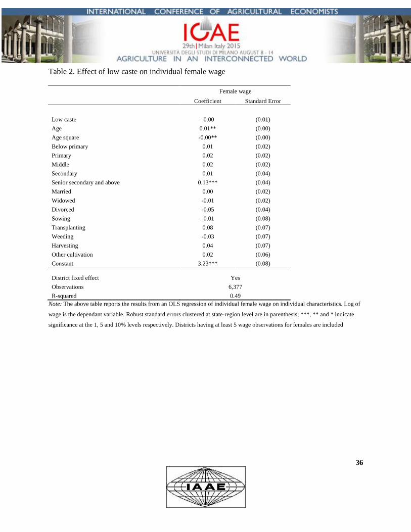
However, the disinclination of higher-caste women to work suggests that their reservation

wage ought to be higher. Table 2 shows the results for the regression of individual female wages

on a dummy for low caste and other controls. The low caste dummy is insignificant controlling

for age, education, marital status, type of agricultural operation and district fixed effects. If the

district fixed effects are dropped, then the low caste dummy is negative and significant even with

other district controls. These controls do not, however, capture the across district variation in

male and female labor supply all of which are impounded in the district fixed effects. Thus,

within a district, differential selection into the labor force does not matter across castes.8

The second concern with caste composition as an instrument is that areas with greater

low-caste households may have lower access to inputs, public goods and infrastructure (Banerjee

and Somanathan 2007). Such areas may also have agro-ecological endowments which are

unfavorable to agriculture. For these reasons, we include a comprehensive set of controls for

irrigation, education, infrastructure (roads, electrification, banks), urbanization and agro-climatic

endowments.

While there is no ex-ante way of knowing whether our controls are good enough, we can

perform the following consistency check. Suppose conditional on our controls, the instrument is

still correlated with omitted variables that affect the demand for agricultural labor. Then the caste

composition also ought to have an effect on the demand for male labor. This can be easily

8 In another set of regressions, we control for the interaction of caste with the education and the age of an individual.

The earnings for low caste women are lower than that of others for educations levels of graduate and higher.

14

checked from the first-stage regressions of the instrument variable procedure. As will be shown

later, conditional on controls for agro-climatic endowments and infrastructure, caste composition

does not have a statistically significant effect on the employment of male labor in agriculture.

A third possibility is that the caste composition in a district reflects long run development

possibilities. In this story, the `higher’ castes used their dominance to settle in better endowed

regions. Once again, this would require adequate controls for agro-ecological conditions. Finally,

could caste composition itself be influenced by wages? Anderson (2011) argues that village level

caste composition in India has remained unchanged for centuries and location of castes is

exogenous to current economic outcomes. This is, of course, entirely consistent with the low

levels of mobility in India noted earlier.

5.2 Identification of the Impact of Male Labor Supply

For male labor supply, this paper uses, as instrument, the district proportion of men (in

the age group 15-59) employed in non-farm manufacturing and mining units with a workforce of

at least 20. The relation between this instrument and district level male employment in

agriculture is plotted in figure 5. The negative association visible in the graph is consistent with

the proposition that competition from non-farm jobs reduces labor supply to agriculture and

increases wages (Lanjouw and Murgai 2009). Rosenzweig’s (1978) study of agricultural labor

markets also uses indicators of non-farm economy as an instrument for labor supply to

agriculture.9 However, not all non-farm activity can be considered to be exogenous to

agriculture. We define our instrument to include employment in manufacturing and mining

sectors, and further restrict it to only large scale units. Our case, elaborated below, is that

employment in the non-traded sectors and in small enterprises is endogenous to agricultural

development but that is not so for large enterprises in traded sectors.

The rural non-farm sector is known to be heterogeneous. Some non-farm activity is of

very low productivity and “functions as a safety net – acting to absorb labor in those regions

9 The variables used by Rosenzweig are the number of factories and workshops per household, percentage of

factories and workshops employing five or more people and the percentage of factories and workshops using power.

15

where agricultural productivity has been declining – rather than being promoted by growth in the

agricultural sector” (Lanjouw and Murgai 2009). These are typically service occupations with

self-employment and limited capital. It is clear that such non-farm activity is endogenous to

agricultural wages.

The other case is when a prosperous agriculture stimulates demand for non-farm activity.

This type of non-farm employment tends to be concentrated in the non-traded sector of retail

trade and services and mostly in small enterprises. Using a village level panel data set across

India, Foster and Rosenzweig (2003) argue that non-traded sectors are family businesses with

few employees while factories are large employers and frequently employ workers from outside

the village in which they are located. In a companion paper, they state that on an average non-

traded service enterprises consist of 2-3 workers. This is no different from the international

experience of developing countries (World Bank 2008, Chapter 9).

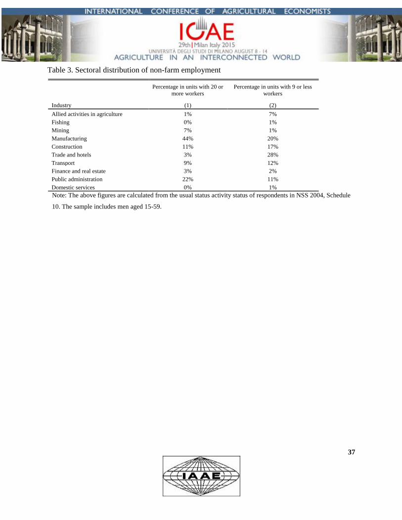
Column 1 in table 3 presents the sectoral distribution of non-farm employment in

production units with workforce of size 20 or more. This can be compared to the sectoral

distribution of non-farm employment in production units with workforce of size nine or less in

column 2 of table 3. It can be seen that, manufacturing and mining account for a substantially

larger proportion of large work units while non-tradable sectors such as trade and hotels,

transport and construction are less important. These considerations dictate that a valid instrument

that captures withdrawal of labor from farm sector would measure non-farm employment in

large units and in the traded sectors.

Even though the tradable non-farm goods and services do not depend on local demand,

this variable could still be invalid if large non-farm enterprises locate in areas of low agricultural

wages. This possibility is suggested in the work of Foster and Rosenzweig (2004). They analyze

a panel data set over the period 1971-1999 collected by the National Council of Applied

Economic Research (NCAER). This data suggests a much higher expansion of rural non-farm

activity than that implied by the nationally representative employment survey data of NSS

(Lanjouw and Murgai 2009). To see if the non-farm sector gravitates towards agriculturally

16

depressed areas in this data set, Lanjouw and Murgai (2009) estimate the impact of growth in

agricultural yields on growth in non-farm sector employment. They take growth in agricultural

yields as a proxy for agricultural productivity and do not find a negative relationship between

manufacturing employment and yield growth. They find a positive association between the two

in the specification with state fixed effects and no other district controls. However, the addition

of region fixed effects makes the positive relation also disappear.

Therefore, if anything, the traded non-farm sector grew more in areas that were relatively

agriculturally advanced. One explanation for this has been provided by Chakravorty and Lall

(2005). They analyze the spatial location of industries in India in the late 1990s and find that

private investment gravitates towards already industrialized and coastal districts with better

infrastructure. No such pattern is seen for government investment. The significance of

geographical clusters is that it makes initial conditions of agricultural productivity and

infrastructure important in determining future investments. This implies that estimation of labor

demand equation should include adequate controls for infrastructure to sustain the validity of the

instrument.

Again, the adequacy of controls that ensures validity of the non-farm employment

instrument may be hard to judge ex-ante. However, if non-farm employment instrument is

correlated with omitted variables that affect overall agricultural labor demand, then the

instrument ought to be significant in the first-stage regression for female employment. As we

show later, this consistency check shows that non-farm employment in large manufacturing and

mining units is not a significant explanatory variable for female employment in agriculture.

6. Data

The key data this paper uses is from the nationally representative Employment and

Unemployment survey of 2004/05 conducted by NSS. The survey contains labor force

participation and earnings details for a reference period of a week. Some of the other variables

including the instruments are also constructed from this data set. The control variables are

obtained from a variety of sources (see Appendix A.1).

17

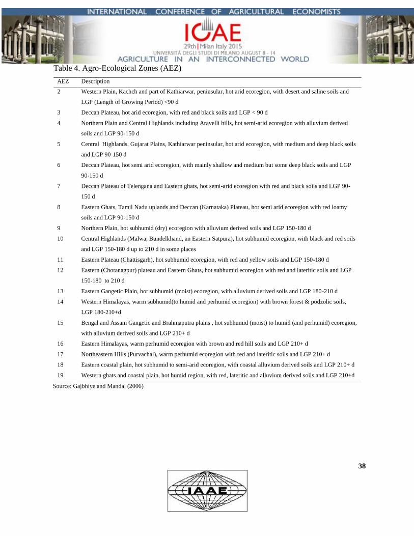
The first set of control variables relate to agriculture: irrigation, inequality in land

holdings, rainfall, agro-climatic endowments, and land allocation to various crops. The agro-

climatic variables are derived from a classification of the country into 20 agro-ecological zones

(AEZ) described in table 4 (Palmer-Jones and Sen 2003). The independent variables are

computed by taking the proportion of area of a district under a particular AEZ. A second set of

control variables relate to infrastructure: roads, electrification and banking. A third set of

variables relate to education and urbanization. Table 5 contains a description of all the variables,

their definitions and descriptive statistics.

The district-level regressions are weighted by district population and the standard errors

are robust and corrected for clustering at state-region level. In some districts, there are very few

wage observations. To avoid the influence of outliers, the districts where the number of wage

observations for either males or females was less than 5 were dropped from the analysis.

Dropping districts where either male or female observations are few in number results in a data

set with equal observations for males and females. However, this could lead to a biased sample

as the districts where female participation in the casual labor market is the least are most likely to

be excluded from the sample. To see whether such selection matters, we also estimate male labor

demand function for districts in which number of male wage observations are at least five

(ignoring the paucity, if any, in the number of female observations) and similarly estimate female

labor demand function for districts in which number of female wage observations are at least five

(ignoring the paucity, if any, of male wage observations).

7. Main Findings

Table 6(a) shows the system two stage least squares(2SLS) estimates of inverse demand

functions for total male and female labor in agriculture. The first specification considers only the

agriculture controls of irrigation, land inequality, rainfall, agro-ecological endowments and

allocation of land to various crops. In the second specification, we add the infrastructure controls

of roads, electrification and banking. The final specification includes the controls for education

and urbanization. Table 6(b) shows the coefficients of the instruments in the first-stage reduced

18

form regressions for each of these three specifications. Table 6(c) displays the coefficients of the

labor supply variables from an ordinary least squares regression.

In Table 6(b), for all specifications, we find a significantly positive association between

proportion of low caste households in a district and female employment in agriculture. Similarly,

a greater presence of large scale non-farm enterprises in manufacturing and mining sectors

decreases male employment in agriculture significantly in all the specifications. The F-statistic

for the instruments is reported in the bottom of table 6(a) and it is significant at five percent level

for female labor supply and at one percent level for male labor supply. The first-stage regressions

thus confirm the causal story about these variables: that status norm govern female labor supply

and that non-farm opportunities are primarily received by men.

Note also that the proportion of low caste households does not affect employment of male

labor in agriculture and presence of large scale non-farm manufacturing and mining enterprises

does not affect female labor employment in agriculture significantly. The significance of this

observation is that if, despite the controls, the instruments retained some residual correlation with

demand for agricultural labor, then we would expect both instruments to be significant in both

the first-stage reduced form regressions. The fact that this is not so supports the case that these

are valid instruments for labor supply to agriculture. Returning to the labor demand equations,

the system 2SLS estimates of the effect of female and male labor supply on own wage rates in

table 6(a) are larger in magnitude and statistically more significant than the OLS estimates in

table 6(c), and have the expected negative signs for own effects. 10 The coefficients of the labor

supply variables do not change much between the three specifications in table 6(a). The

agriculture controls seem to be the most important in removing the correlation between

agricultural labor demand and the instruments.

The cross effects of labor supply on wage rates are negative in sign. This implies that

males and females are substitutes in agriculture. However, male labor and female labor are not

perfect substitutes. In the system 2SLS regressions with full set of controls (the third

10

By the Durbin-Wu-Hausman test, the null hypothesis that the employment variables can be treated as exogenous

is rejected for all specifications (at 10 % significance level).

19

specification), female labor supply has a significant impact on female wage with an inverse

demand elasticity of – 0.52. However, the impact of female labor supply on male wage is

smaller (around -0.1) and is not significantly different from zero. Thus, an increase in female

labor supply by 10% decreases female wage by 5.2%, male wage by 1.3% and decreases the

female to male wage ratio by 4%. To test formally that the impact on female wage is greater (in

absolute terms) than the impact on male wage, we carry out a chi-square-test. In all of the

specifications, the chi-square-test rejects the null that the coefficients are equal against the

alternative that the coefficient of female labor supply in the female wage regression is higher

than the coefficient of female labor supply in the male wage regression. This is supportive of the

Boserup hypothesis that the caste driven variation in female labor supply leads to variation in the

gender wage gap in agriculture across regions of India. In particular, greater female work

participation decreases female wage relative to male wage.11

In contrast, the effect of male labor supply variation is significant for both male and

female wage rates. In the third specification with the full set of controls, the point estimate of the

inverse demand elasticity is -0.37 for female and -0.28 for male wage with respect to male labor

supply. Although large scale non-farm employment is dominated by men, non-farm labor

demand has favorable effects on female and male wage rates. The point estimates would imply

that a 10% decrease in male labor supply increases male wage by 2.8%, female wage by 3.7%

and increases the female to male wage ratio by one percent. A chi-square test however, does not

reject (in all the specifications) the null of equality of the two coefficients in the male and female

inverse demand functions for male labor supply. Hence, a decrease in male labor supply to

agriculture has no significant impact on gender wage gap in agriculture.

11

We also estimated the Rosenzweig specification for our data set with instruments that are as close as possible to

those employed by him. In these results, the female labor supply has a significant negative impact on both female

and male wages but not on the gender wage gap. This matches the finding of Rosenzweig for the 1961 data. We also

find that male labor supply does not have a significant impact on the gender wage gap even though the impact on

male wages is significant and negative and insignificant for female wages. In Rosenzweig’s earlier analysis, male

labor supply had an insignificant impact on male and female wages and therefore did not matter to the gender wage

gap.

20

There is, thus, an asymmetry between the effects of gender specific variation in labor

supply on the wage of the opposite gender. Male labor supply matters to female wage but the

effect of female labor supply on male wage is small and insignificant. Why is this so? The

theoretical model posited in section 3 predicts that the elasticity of female wage with respect to

male labor supply relative to the similar cross elasticity of male wage is the product of two

ratios: the ratio of male to female labor employment and the male to female wage ratio. The

sample estimate of male and female labor employment is 5.17 and 2.57 days per week per

hectare of land respectively while the sample estimate for male and female wage is Rs 47.3 and

Rs 36.13 per day respectively. This gives an estimate of relative cross-wage elasticities to be

2.63. The results in table 6(a), for the specification with the full set of controls, yield an

econometric estimate of the ratio of cross-wage elasticities as 2.84 which is close to the

prediction from the theoretical model.

The control variables (i.e., other than the labor supply variables) could also have an effect

on the gender wage gap. To ascertain this, a chi-square test was conducted to test for the equality

of coefficients for each control variable across male and female demand equations. The null

hypothesis of equality of coefficients is rejected at the five percent level of significance for rice

cultivation, access to roads and landholding inequality. Rice growing areas have a higher

demand for female labor which leads to a higher wage rate for women and translates into a lower

gender wage gap. Many researchers have documented greater demand for female labor in rice

cultivation due to greater demand for females in tasks like transplanting and weeding (Mbiti

2007) and this result validates their observations. On the other hand, access to roads seems to

increase demand for only male labor resulting in a larger wage gap between females and males in

districts with better access to roads. Landholding inequality measured by the Gini coefficient for

a district affects demand for both males and females significantly negatively reflecting the well

known feature that large farms use less labor per unit of land than small farms. However, women

are more adversely affected by men resulting in a larger gender wage gap in districts with higher

land inequality. Theoretically, the effect of landholding inequality on gender wage differential is

ambiguous (Rosenzweig 1978).

21

A concern with the 2SLS results is that the first-stage F-statistic though significant is not

very large. Weak-instruments could lead to biased estimates and to finite sample distributions

that are poorly approximated by the theoretical asymptotic distribution. While such concerns are

greater in an over-identified model, the weak-instrument critique suggests caution in interpreting

the 2SLS results. As a check for just identified models with possibly weak-instruments, Angrist

and Pischke (2008) and Chernozhukov and Hansen (2008) recommend looking at the reduced

form estimates (of the dependent variable on all exogenous variables) since they have the

advantage of being unbiased. Chernozhukov and Hansen (2008) formally show that the test for

instrument irrelevance in this reduced form regression can be viewed as a weak-instrument-

robust test of the hypothesis that the coefficient on the endogenous variable in the structural

equation is zero. The sign and the strength of the coefficients in the reduced form regression can

provide evidence of whether a causal relationship exists.

Table 6(d) shows the results for the coefficients of instruments from the reduced form

regression of male and female wage on instruments and other covariates. The instruments are

significant in this regression and so it can be concluded that the weak-instrument problem does

not contaminate the inference from the structural regressions. It can be seen that an increase in

proportion of low caste households reduces only the female wage. This is entirely consistent with

the 2SLS results where the instrument increases only female labor supply (the first-stage

regression) which in turn has a significantly negative impact only on female wage. On the other

hand, large scale industrial employment has a significantly positive impact on male and female

wage rates. This is also in line with the 2SLS results where the presence of large enterprises in

the non-farm sector decreases only male labor supply to agriculture which in turn impacts both

male and female wage positively.

8. Robustness checks

The third specification in table 6(a) is our baseline and we consider the robustness of its

estimates. Table 7(a) adds more agriculture controls: fertilizers per unit of cultivated land and

implements (consisting of tractor and power operated tools) per unit of cultivated land. Including

22

fertilizers (first two columns) does not change the impact of female labor supply on male and

female wage and a 10% increase in female labor supply increases the gender wage gap by 3.6%.

The chi-square test does not reject the equality of male labor supply coefficients across male and

female labor demand equations but rejects the equality of female labor supply coefficients. The

inclusion of fertilizers does, however, reduce the coefficient of irrigation in both equations to the

point that it becomes insignificant in the female labor demand equation. This is possibly because

of a high positive correlation (0.4) between irrigation and fertilizer use. Controlling for

implements used per unit land cultivated (column 3 and 4) does not change any of the principal

findings of the base specification. Again, the chi-square test does not reject the equality of male

labor supply coefficients across male and female demand equations but rejects the equality of

female labor supply coefficients.

In a third robustness check, we control for male and female health in rural areas.

Nutrition status can affect productivity which in turn could impact rural wage. If nutrition status

is correlated with our instrumental variable of low caste composition, then it could bias our

results as well. Adult measures of health in India are not available at district level. Weight and

height measurements are available at state level from the National Family and Health Survey of

2005-06. The measure of under-nutrition is percentage of rural adults with a body mass index of

less than 18.5. Table 7(b) shows the structural estimates for the total demand for labor with state

level health controls. The results from the base specification continue to hold. While increase in

female labor supply increases the gender wage gap significantly, male labor supply has no

impact.

As a fourth check, we reconsider our sample selection rule. Recall, that we chose districts

for which there were at least five observations for female as well as male wages. While this

ensures an equal sample size for males and females, it also entails a risk of dropping districts

where female participation in wage work is the least. To check robustness, we consider the

following alternative. For the male worker sample, we considered all districts where there are at

least five observations for male wages. Similarly, for the female worker sample, we included all

districts where there are at least five observations for female wages. This increases the number of

23

districts from 279 in the matched sample to 359 for males and to 288 for females. Table 8 shows

the estimates from the baseline specification on this enlarged sample. The estimates validate our

central result that the gender wage gap is sensitive to female labor supply and not to male labor

supply. In fact, the effect of female labor supply on gender wage gap in the enlarged sample is

greater. A 10% increase in female labor supply results in a 4.8% decline in female to male wage

ratio in the enlarged sample compared to 4% in the matched sample.

In a fifth robustness check, we control for differential participation in tasks by males and

females across districts. As noted earlier, some agricultural tasks are traditionally deemed as

male while others are dominated by women. In section 3, we showed that the gender wage gap in

Indian agriculture is within tasks. A very small percentage of the wage gap can be attributed to

differential participation of men and women across tasks. To address this issue formally, we

regress individual wages on individual characteristics (age, age square, education dummies, and

marital status dummies), district level female and male labor employment in agriculture (suitably

instrumented), other district controls and dummy variables for agricultural tasks for which the

wage is recorded. The agricultural tasks are ploughing, sowing, transplanting, weeding,

harvesting and other agricultural activities.

The estimates are reported in table 9(a). They show that a 10% increase in female labor

supply reduces female wage by 5.5% and has no significant effect on male wage. Male labor

supply on the other hand has an identical negative effect on male and female wage.

Lastly, we consider the possibility that hired and family labor may not be equally

efficient. Family labor may be more efficient because of better incentives. If this is so, a simple

aggregate of family and hired labor is not valid and could lead to inconsistent estimates.

Suppose one unit of hired labor is equivalent to units of family labor (with less than one).

Then in terms of efficiency units of family labor, the total labor supply is

, where

and are the aggregate labor supply to home farm and to outside farms. In the regressions, we

have measured labor supply as

. Since,

= ln

+ ln[(

, the second term is absorbed in the error term of the regressions. This could

24

lead to inconsistent estimates. The instruments will be correlated with

if they not

only affect the total labor supply but also the allocation of labor between own farm and outside

farm. It is possible that low caste women have a greater propensity to work outside their family

farm due to less social restrictions. Similarly, the opportunity of employment in manufacturing

and mining could lead landed households to divert their labor supply to industry and increase

hiring of labor on their farms.

To meet these concerns, we estimate the baseline specification for values of ={0.5, 0.7,

0.9}, for both male and female labor. The results are shown in table 10. The last column shows

the results with =1 which corresponds to the results of the base specification in table 6(a). As

the value of decreases, the impact of female labor supply on male wage does not change but

the impact of female labor supply on female wage falls in magnitude. The chi-square test for the

equality of the impact of female labor supply on female and male wage continues to be rejected

for the selected values of . A decrease in the value of increases the impact of male labor

supply on both male and female wage. Once again, the chi-square test for the equality of the

impact of male labor supply on male and female wage is not rejected for the selected values of .

9. Explaining the difference in wage gap between northern and southern states of India

While our findings support the Boserup hypothesis, there are other factors as well that

matter to the gender wage gap. So to what extent does the Boserup hypothesis, i.e., the difference

in female work participation across northern and southern states in India explain the observed

difference in the gender wage gap?

From estimation equations (8a) and (8b), the gender wage gap in a southern state can be

written as

where, W is the log of wages, L is the log of labor supply and X are other district level covariates

included in the empirical analysis. ‘M’ and ‘F’ index males and females respectively. Similarly,

the gender wage gap in a northern state can be written as

25

Subtracting 10 from 9, we obtain

The ratio is the proportion of the

difference in wage gap across north and south that is explained by the difference in female labor

supply.

To implement this, we let the variables take the average values of northern and southern

states respectively.12 The mean values are listed in table 11. The parameters are drawn from the

coefficient estimates of the base specification estimated in column 3 of Table 6(a). Table 12

shows the proportion of the gender wage gap explained by each right hand side variable. The

proportions for agro-ecological zones have not been shown for brevity. One can see that 55

percent of the regional difference in the gender wage gap is because of the larger female labor

supply in the southern states. Greater land inequality and lower area under cultivation of rice in

the southern states are other important and significant factors which lead to a greater gender

wage gap in the south. On the other hand, greater electrification, lower male supply and the

greater importance of coarse cereal crops (sorghum and millets) should lead to a lower wage gap

in the south but these do not affect the gender wage gap significantly in the regressions.

10. Conclusion

The effect of variation in female work force participation on the gender wage gap in

developed countries has been explored in recent papers. In a developing country context, such a

12

We classify Andhra Pradesh, Karnataka, Kerala, Maharashtra and Tamil Nadu as southern states while Punjab,

Haryana, Uttar Pradesh, Bihar, Gujarat, Rajasthan, Madhya Pradesh, West Bengal and Assam are classified as

northern states. Orissa is omitted from the north-south analysis since it does not fall clearly into any of the categories

and also is geographically sandwiched between the north and the south.

26

connection was made by Boserup many decades ago. Based on data from 1950s, she posited that

the gender wage gap was higher in the southern states of India relative to the northern states

because of greater female labor supply in south India, which stemmed from differences in

cultural restrictions on women’s participation in economic activity. This paper confirms the

hypothesis within a neo-classical framework of labor markets. Compared to the literature, this

paper also pays attention to the variation in male labor supply and how that impacts the gender

wage gap. The exogenous variation in labor supply was identified by spatial variation in caste

composition and non-farm employment of men in large units.

We find that female labor supply has a sizeable effect on female wage but not so much on

male wage. This result thus has important implications for the literature on gender wage

differentials. It shows that the usual approach of attributing the gender wage gap to only

individual characteristics or discrimination is incomplete. The overall labor market structure that

determines labor supply and the substitutability between female and male labor may also have a

significant impact on gender wage inequality.

The paper also found that male labor supply has sizeable effects on male as well as

female wage. This finding is interesting on three counts. First, it provides a causal effect of

withdrawal of males from agriculture due to non-farm employment opportunities on wages of

men and women. The paper, therefore, sheds light on the economic processes that affect

agricultural wage (Lanjouw and Murgai 2009; Eswaran et al. 2009; Foster and Rosenzweig

2003). Second, the strong effect of male labor supply on female wage is of independent interest

since the sectoral mobility of women from the farm to the non-farm sector is much less marked

compared to men (Eswaran et al. 2009). This could be because of lower education levels as well

as societal constraints that limit female participation in most non-farm jobs. This raises a concern

that rapid growth in the non-farm sector does not entail much gain for women. Our finding,

however, suggests that there is enough substitutability between men and women in the

agricultural production process that a withdrawal of men from agriculture has positive effects on

male and female wages.

27

Finally, the findings point to a marked asymmetry between the effects of female and male

labor supply. Female labor supply does not impact male wage significantly but male labor supply

does move female wage significantly. A standard neo-classical model predicts this asymmetry

and its magnitude is determined by the gender gap in wage and the gender gap in labor supply.

The findings match the prediction closely.

References

Acemoglu, Daron, Autor, David H., and David Lyle. 2004. “Women, War, and Wages: The

Effect of Female Labor Supply on the Wage Structure at Mid-Century.”Journal of Political

Economy 112, no. 3:497-551.

Aggarwal, Bina. 1994. A Field of One’s Own: Gender and Land rights in South Asia.

Cambridge: Cambridge University Press.

Aldrich, Mark. 1989. "The gender gap in earnings during World War II: New evidence."

Industrial and Labor Relations Review 42, no. 3:415-429.

Anderson, Siwan. 2011. “Caste as an Impediment to Trade.” American Economic Journal:

Applied Economics 3, no.1:239-263.

Angrist, Joshua D., and Jorn-Steffen Pischke. 2008. Mostly harmless econometrics: An

empiricist's companion. Princeton University Press.

Bagchi, Deipica, and Saraswati Raju. 1993. Women and work in South Asia. London:

Routledge.

Banerjee, Abhijit, and Rohini Somanathan. 2007. “The political economy of public goods: Some

evidence from India.” Journal of Development Economics 82: 287–314.

Bardhan, Kalpana. 1984. “Work Patterns and Social Differentiation: Rural Women of West

Bengal.” In Contractual Arrangements, Employment and Wages in Rural Labor Markets in Asia,

ed. Hans P. Binswanger andMark R. Rosenzweig. New Haven, pp. 184-208.

29

Bardhan, Pranab K. 1984. “Determinants of supply and demand for labor in a poor agrarian

economy: an analysis of household survey data from rural West Bengal.” In Contractual

Arrangements, Employment and Wages in Rural Labor Markets in Asia, ed. Hans P. Binswanger

and Mark R. Rosenzweig. New Haven, pp. 242-262.

Basu, Alaka M. 1992. Culture, the Status of Women, and Demographic Behaviour: Illustrated

with the Case of India. Oxford: Clarendon Press.

Beteille, Andre. 1969. Caste, Class and Power: Changing Patterns of Stratification in a Tanjore

Village. University of California Press.

Blau, Francine D., and Lawrence M. Kahn. 2003. “Understanding International Differences in

the Gender Pay Gap.” Journal of Labor Economics 21, no. 1:106-144.

Boserup, Ester. 1970. Women's role in economic development. New York: St. Martin'.

Burton, Michael L., and Douglas R. White. 1984. “Sexual division of labor in agriculture.”

American Anthropologist 86, no. 3:568–583.

Cameron, Lisa A., Dowling, J. Malcolm, and Christopher Worswick. 2001. “Education and

Labor Market Participation of Women in Asia: Evidence from Five Countries.” Economic

Development and Cultural Change 49, no. 3:459-477.

Chakravorty , Sanjoy, and Somik Vinay Lall. 2005. “Industrial Location and Spatial Inequality:

Theory and Evidence from India.” Review of Development Economics 9, no. 1:47–68.

30

Chen, Martha. 1995. “A Matter of Survival: Women’s Right to Employment in India and

Bangladesh.” In Women, culture and development: a study of human capabilities, ed. Martha C.

Nussbaum and Jonathan Glover. Oxford, pp. 37-59.

Chernozhukov, Victor, and Christian Hansen. 2008. “The reduced form: A simple approach to

inference with weak instruments.” Economics Letters 100, no. 1:68-71.

Das, Maitreyi Bordia. 2006. “Do Traditional Axes of Exclusion Affect Labor Market Outcomes

in India?” Social Development Papers, South Asia Series, Paper no. 97.

Das, Maitreyi Bordia, and Puja Vasudeva Dutta. 2008. “Does caste matter for wages in the

Indian labor market?” Draft paper, World Bank, Washington, DC.

Datt, Gaurav. 1996. Bargaining power, wages and employment: an analysis of agricultural labor

markets in India. New Delhi: Sage Publications.

Doss, Cheryl R. 1999. “Twenty Five Years of Research on Women Farmers in Africa: Lessons

and Implications for Agricultural Research Institutions: with an Annotated Bibliography.”

CIMMYT Economics Program Paper No. 99-02, Mexico.

Dyson, Tim, and Mick Moore.1983. “On kinship structure, female autonomy, and demographic

behavior in India.” Population and Development Review 9, no. 1:35–60.

Eswaran, Mukesh, Kotwal, Ashok, Ramaswami, Bharat, and Wilima Wadhwa. 2009. “Sectoral

Labor Flows and Agricultural Wages in India, 1982-2004: Has Growth Trickled Down?”

Economic and Political Weekly 44, no. 2:46–55.

31

Eswaran, Mukesh, Ramaswami, Bharat, and Wilima Wadhwa. 2013. “Status, Caste, and the

Time Allocation of Women in Rural India.” Economic Development and Cultural Change 61,

no. 2:311-333.

Foster, Andrew D., and Mark R. Rosenzweig. 2003. “Agricultural development, industrialization

and rural inequality.” Unpublished, Cambridge, Massachusetts, Harvard University.

-----------------------. 2004. “Agricultural Productivity Growth, Rural Economic Diversity, and

Economic Reforms: India, 1970–2000.” Economic Development and Cultural Change 52, no.

3:509-542.

Gajbhiye, K.S., and C. Mandal. 2006. “Agro-Ecological Zones, their Soil Resource and

Cropping Systems.” National Bureau of Soil Survey and Land Use Planning, Nagpur.

Goldin, Claudia. 1995. "The U-Shaped Female Labor Force Function in Economic Develop-

ment and Economic History." In Investment in Women's Human Capital, ed. T. Paul Schultz.

Chicago: University of Chicago Press.

Hertz, Tom, Campos, Ana P., Zezza, Alberto, Azzarri, Carlo, Winters, Paul, Quinones, Esteban

J., and Benjamin Davis. 2009. “Wage Inequality in International Perspective: Effects of

Location, Sector, and Gender.” Paper presented at the FAO-IFAD-ILO Workshop on Gaps,

trends and current research in gender dimensions of agricultural and rural employment:

differentiated pathways out of poverty, Rome, March 31- April 2.

Himanshu. 2005. “Wages in Rural India: Sources, Trends and Comparability.” Indian

Journal of Labor Economics 48, no. 2:375-406.

32

Jacoby, Hanon G. 1992. “Productivity of men and women and the sexual division of labor in

peasant agriculture of the Peruvian Sierra.” Journal of Development Economics 37, no. 1-2:265-

287.

Jayachandran, Seema. 2006. “Selling labor low: Wage responses to productivity shocks in

developing countries.” Journal of Political Economy 114, no. 3:538–575.

Jejeebhoy, Shireen J. 2001. “Women’s autonomy in rural India: Its dimensions, determinants,

and the influence of context.” In Women’s Empowerment and Demographic Processes: Moving

Beyond Cairo, ed. Harriet Presser and Gita Sen. Oxford, pp. 205-238.

Kanwar, Sunil. 2004. “Seasonality and Wage Responsiveness in a Developing Agrarian

Economy.” Oxford Bulletin of Economics and Statistics 66, no. 2:189-204.

Lanjouw, Peter, and Rinku Murgai. 2009. “Poverty decline, agricultural wages, and non-farm

employment in rural India: 1983-2004.” Agricultural Economics 40, no. 2:243-263.

Laufer, Leslie A. 1985. “The Substitution between Male and Female Labor in Rural Indian

Agricultural Production.” Economic Growth Center Discussion Paper No. 472, New Haven, CT:

Yale University.

Mammen, Kristin, and Christina Paxson. 2000. “Women's Work and Economic Development.”

The Journal of Economic Perspective 14, no. 4:141-164.

Mbiti, Isaac M. 2007. “Moving Women: Household Composition, Labor Demand and Crop

Choice.” Unpublished paper, Department of Economics, Southern Methodist University, Dallas,

TX, USA.

33

Mitra, Arup, and Mayumi Murayama. 2008. “Rural to Urban Migration: A District Level

Analysis for India.” IDE Discussion Paper 137.

Munshi, Kaivan, and Mark R. Rosenzweig. 2009. “Why is mobility in India so low? Social

insurance, inequality, and growth.” NBER Working Paper No. 14850.

Nayyar, Rohini. 1987. “Female Participation Rates in Rural India.” Economic and Political

Weekly 22, no. 51:2207-2216.

Palmer-Jones, Richard, and Kunal Sen. 2003. “What has luck got to do with it? A regional

analysis of poverty and agricultural growth in rural India.” Journal of Development Studies 40,

no. 1:1-31.

Parida, Jajati Keshari, and S. Madheswaran. 2010. “Spatial Heterogeneity and Population

Mobility in India.” Institute for Social and Economic Change Working Paper 234.

Quisumbing, Agnes R. 1996. “Male-Female Differences in Agricultural Productivity:

Methodological Issues and Empirical Evidence.” World Development 24, no. 10:1579-1595.

Rahman, Lupin, and Vijayendra Rao. 2004. “The Determinants of Gender Equity in India:

Examining Dyson and Moore's Thesis with New Data.” Population and Development Review 30,

no. 2:239-268.

Rajaraman, Indira. 1986. “Offered wage and recipient attribute: Wage functions for rural labor in

India.” Journal of Development Economics 24, 179-195.

34

Rao, V. M. 1972. “Agricultural Wages in India – A Reliability Analysis.” Indian Journal of

Agricultural Economics 27, no. 3:39-61.

Rosenzweig, Mark R. 1978. “Rural wages, labor supply, and land reform: A theoretical and

empirical analysis.” American Economic Review 68, no. 5:847-861.

Singh, Ram D. 1996. “Female Agricultural Workers' Wages, Male-Female Wage differentials,

and Agricultural Growth in a Developing Country, India.” Economic Development and Cultural

Change 45, no. 1:89-123.

Skoufias, Emmanuel. 1993. “Seasonal Labor Utilization in Agriculture: Theory and Evidence

from Agrarian Households in India.” American Journal of Agricultural Economics 75, no. 1:20-

32.

Tumbe, C. 2014. “The Great Indian Migration Wave, 1870-2010, Persistence & Consequences.”

Mimeo

World Bank. 2007. “World development report 2008: Agriculture for development.”

http://siteresources.worldbank.org/INTWDR2008/Resources/WDR_00_book.pdf (accessed September

24, 2013).

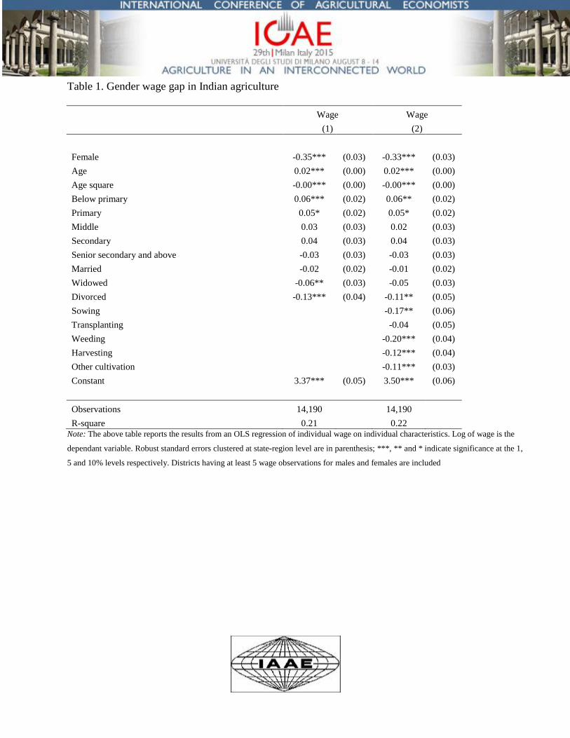
Table 1. Gender wage gap in Indian agriculture

Wage Wage

(1) (2)

Female -0.35*** (0.03) -0.33*** (0.03)

Age 0.02*** (0.00) 0.02*** (0.00)

Age square -0.00*** (0.00) -0.00*** (0.00)

Below primary 0.06*** (0.02) 0.06** (0.02)

Primary 0.05* (0.02) 0.05* (0.02)

Middle 0.03 (0.03) 0.02 (0.03)

Secondary 0.04 (0.03) 0.04 (0.03)

Senior secondary and above -0.03 (0.03) -0.03 (0.03)

Married -0.02 (0.02) -0.01 (0.02)

Widowed -0.06** (0.03) -0.05 (0.03)

Divorced -0.13*** (0.04) -0.11** (0.05)

Sowing

-0.17** (0.06)

Transplanting

-0.04 (0.05)

Weeding

-0.20*** (0.04)

Harvesting

-0.12*** (0.04)

Other cultivation

-0.11*** (0.03)

Constant 3.37*** (0.05) 3.50*** (0.06)

Observations 14,190

14,190

R-square 0.21 0.22 Note: The above table reports the results from an OLS regression of individual wage on individual characteristics. Log of wage is the

dependant variable. Robust standard errors clustered at state-region level are in parenthesis; ***, ** and * indicate significance at the 1,

5 and 10% levels respectively. Districts having at least 5 wage observations for males and females are included

36

Table 2. Effect of low caste on individual female wage

Female wage

Coefficient Standard Error

Low caste -0.00 (0.01)

Age 0.01** (0.00)

Age square -0.00** (0.00)

Below primary 0.01 (0.02)

Primary 0.02 (0.02)

Middle 0.02 (0.02)

Secondary 0.01 (0.04)

Senior secondary and above 0.13*** (0.04)

Married 0.00 (0.02)

Widowed -0.01 (0.02)

Divorced -0.05 (0.04)

Sowing -0.01 (0.08)

Transplanting 0.08 (0.07)

Weeding -0.03 (0.07)

Harvesting 0.04 (0.07)

Other cultivation 0.02 (0.06)

Constant 3.23*** (0.08)

District fixed effect Yes

Observations 6,377

R-squared 0.49

Note: The above table reports the results from an OLS regression of individual female wage on individual characteristics. Log of

wage is the dependant variable. Robust standard errors clustered at state-region level are in parenthesis; ***, ** and * indicate

significance at the 1, 5 and 10% levels respectively. Districts having at least 5 wage observations for females are included

37

Table 3. Sectoral distribution of non-farm employment

Industry

Percentage in units with 20 or

more workers

Percentage in units with 9 or less

workers

(1) (2)

Allied activities in agriculture 1% 7%

Fishing 0% 1%

Mining 7% 1%

Manufacturing 44% 20%

Construction 11% 17%

Trade and hotels 3% 28%

Transport 9% 12%

Finance and real estate 3% 2%

Public administration 22% 11%

Domestic services 0% 1%

Note: The above figures are calculated from the usual status activity status of respondents in NSS 2004, Schedule

10. The sample includes men aged 15-59.

38

Table 4. Agro-Ecological Zones (AEZ)

AEZ Description

2 Western Plain, Kachch and part of Kathiarwar, peninsular, hot arid ecoregion, with desert and saline soils and

LGP (Length of Growing Period) <90 d

3 Deccan Plateau, hot arid ecoregion, with red and black soils and LGP < 90 d

4 Northern Plain and Central Highlands including Aravelli hills, hot semi-arid ecoregion with alluvium derived

soils and LGP 90-150 d

5 Central Highlands, Gujarat Plains, Kathiarwar peninsular, hot arid ecoregion, with medium and deep black soils

and LGP 90-150 d

6 Deccan Plateau, hot semi arid ecoregion, with mainly shallow and medium but some deep black soils and LGP

90-150 d

7 Deccan Plateau of Telengana and Eastern ghats, hot semi-arid ecoregion with red and black soils and LGP 90-

150 d

8 Eastern Ghats, Tamil Nadu uplands and Deccan (Karnataka) Plateau, hot semi arid ecoregion with red loamy

soils and LGP 90-150 d

9 Northern Plain, hot subhumid (dry) ecoregion with alluvium derived soils and LGP 150-180 d

10 Central Highlands (Malwa, Bundelkhand, an Eastern Satpura), hot subhumid ecoregion, with black and red soils

and LGP 150-180 d up to 210 d in some places

11 Eastern Plateau (Chattisgarh), hot subhumid ecoregion, with red and yellow soils and LGP 150-180 d

12 Eastern (Chotanagpur) plateau and Eastern Ghats, hot subhumid ecoregion with red and lateritic soils and LGP

150-180 to 210 d

13 Eastern Gangetic Plain, hot subhumid (moist) ecoregion, with alluvium derived soils and LGP 180-210 d

14 Western Himalayas, warm subhumid(to humid and perhumid ecoregion) with brown forest & podzolic soils,

LGP 180-210+d

15 Bengal and Assam Gangetic and Brahmaputra plains , hot subhumid (moist) to humid (and perhumid) ecoregion,

with alluvium derived soils and LGP 210+ d

16 Eastern Himalayas, warm perhumid ecoregion with brown and red hill soils and LGP 210+ d

17 Northeastern Hills (Purvachal), warm perhumid ecoregion with red and lateritic soils and LGP 210+ d

18 Eastern coastal plain, hot subhumid to semi-arid ecoregion, with coastal alluvium derived soils and LGP 210+ d

19 Western ghats and coastal plain, hot humid region, with red, lateritic and alluvium derived soils and LGP 210+d

Source: Gajbhiye and Mandal (2006)

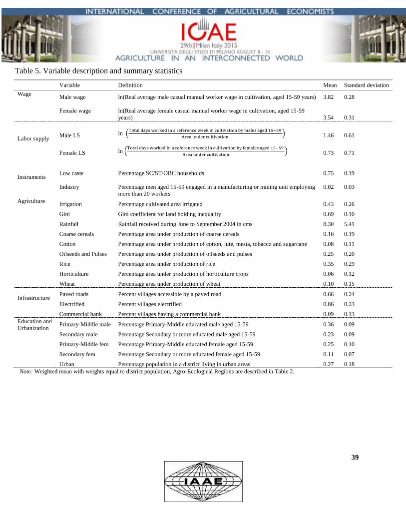
39

Table 5. Variable description and summary statistics

Variable Definition Mean Standard deviation

Wage Male wage ln(Real average male casual manual worker wage in cultivation, aged 15-59 years) 3.82 0.28

Female wage

ln(Real average female casual manual worker wage in cultivation, aged 15-59

years)

3.54 0.31

Labor supply Male LS ln

1.46 0.61

Female LS

ln

0.73 0.71

Instruments Low caste Percentage SC/ST/OBC households 0.75 0.19

Industry

Percentage men aged 15-59 engaged in a manufacturing or mining unit employing

more than 20 workers

0.02

0.03

Agriculture Irrigation Percentage cultivated area irrigated 0.43 0.26

Gini Gini coefficient for land holding inequality 0.69 0.10

Rainfall Rainfall received during June to September 2004 in cms 8.30 5.41

Coarse cereals Percentage area under production of coarse cereals 0.16 0.19

Cotton Percentage area under production of cotton, jute, mesta, tobacco and sugarcane 0.08 0.11

Oilseeds and Pulses Percentage area under production of oilseeds and pulses 0.25 0.20

Rice Percentage area under production of rice 0.35 0.29

Horticulture Percentage area under production of horticulture crops 0.06 0.12

Wheat Percentage area under production of wheat 0.10 0.15

Infrastructure Paved roads Percent villages accessible by a paved road 0.66 0.24

Electrified Percent villages electrified 0.86 0.23

Commercial bank Percent villages having a commercial bank 0.09 0.13

Education and

Urbanization Primary-Middle male Percentage Primary-Middle educated male aged 15-59 0.36 0.09

Secondary male Percentage Secondary or more educated male aged 15-59 0.23 0.09

Primary-Middle fem Percentage Primary-Middle educated female aged 15-59 0.25 0.10

Secondary fem Percentage Secondary or more educated female aged 15-59 0.11 0.07

Urban Percentage population in a district living in urban areas 0.27 0.18

Note: Weighted mean with weights equal to district population, Agro-Ecological Regions are described in Table 2.

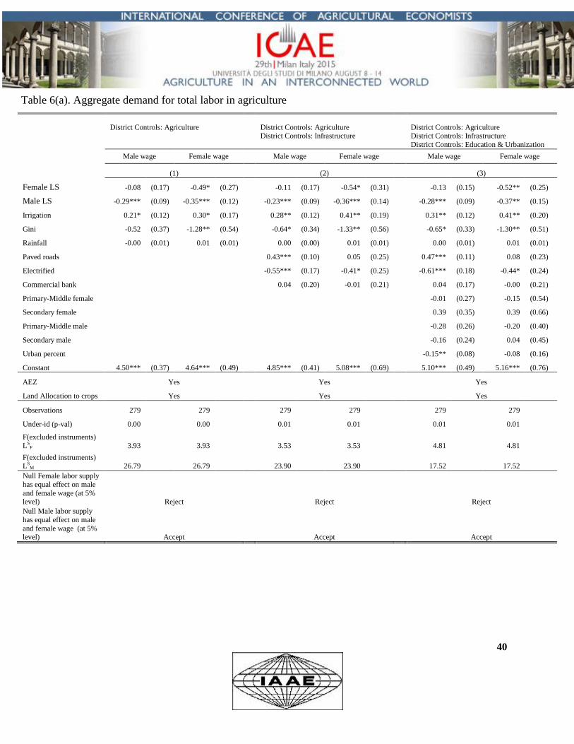
40

Table 6(a). Aggregate demand for total labor in agriculture

District Controls: Agriculture

District Controls: Agriculture District Controls: Infrastructure

District Controls: Agriculture District Controls: Infrastructure

District Controls: Education & Urbanization

Male wage Female wage

Male wage Female wage

Male wage Female wage

(1) (2) (3)

Female LS -0.08 (0.17) -0.49* (0.27)

-0.11 (0.17) -0.54* (0.31)

-0.13 (0.15) -0.52** (0.25)

Male LS -0.29*** (0.09) -0.35*** (0.12)

-0.23*** (0.09) -0.36*** (0.14)

-0.28*** (0.09) -0.37** (0.15)

Irrigation 0.21* (0.12) 0.30* (0.17)

0.28** (0.12) 0.41** (0.19)

0.31** (0.12) 0.41** (0.20)

Gini -0.52 (0.37) -1.28** (0.54)

-0.64* (0.34) -1.33** (0.56)

-0.65* (0.33) -1.30** (0.51)

Rainfall -0.00 (0.01) 0.01 (0.01)

0.00 (0.00) 0.01 (0.01)

0.00 (0.01) 0.01 (0.01)

Paved roads

0.43*** (0.10) 0.05 (0.25)

0.47*** (0.11) 0.08 (0.23)

Electrified

-0.55*** (0.17) -0.41* (0.25)

-0.61*** (0.18) -0.44* (0.24)

Commercial bank

0.04 (0.20) -0.01 (0.21)

0.04 (0.17) -0.00 (0.21)

Primary-Middle female

-0.01 (0.27) -0.15 (0.54)

Secondary female

0.39 (0.35) 0.39 (0.66)

Primary-Middle male

-0.28 (0.26) -0.20 (0.40)

Secondary male

-0.16 (0.24) 0.04 (0.45)

Urban percent

-0.15** (0.08) -0.08 (0.16)

Constant 4.50*** (0.37) 4.64*** (0.49)

4.85*** (0.41) 5.08*** (0.69)

5.10*** (0.49) 5.16*** (0.76)

AEZ Yes Yes Yes

Land Allocation to crops Yes Yes Yes

Observations 279

279

279

279

279

279

Under-id (p-val) 0.00

0.00

0.01

0.01

0.01

0.01

F(excluded instruments)

LSF 3.93

3.93

3.53

3.53

4.81

4.81

F(excluded instruments) LS

M 26.79 26.79 23.90 23.90 17.52 17.52

Null Female labor supply

has equal effect on male

and female wage (at 5% level) Reject

Reject

Reject

Null Male labor supply

has equal effect on male

and female wage (at 5% level) Accept Accept Accept

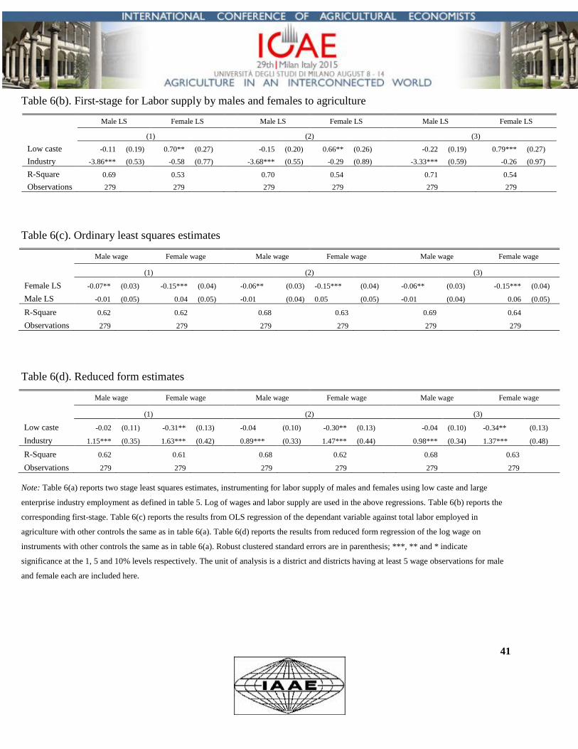
41

Table 6(b). First-stage for Labor supply by males and females to agriculture

Male LS Female LS

Male LS Female LS

Male LS Female LS

(1) (2) (3)

Low caste -0.11 (0.19) 0.70** (0.27)

-0.15 (0.20) 0.66** (0.26)

-0.22 (0.19) 0.79*** (0.27)

Industry -3.86*** (0.53) -0.58 (0.77)

-3.68*** (0.55) -0.29 (0.89)

-3.33*** (0.59) -0.26 (0.97)

R-Square 0.69 0.53 0.70 0.54 0.71 0.54

Observations 279 279 279 279 279 279

Table 6(c). Ordinary least squares estimates

Male wage Female wage

Male wage Female wage

Male wage Female wage

(1) (2) (3)

Female LS -0.07** (0.03) -0.15*** (0.04)

-0.06** (0.03) -0.15*** (0.04)

-0.06** (0.03) -0.15*** (0.04)

Male LS -0.01 (0.05) 0.04 (0.05)

-0.01 (0.04) 0.05 (0.05)

-0.01 (0.04) 0.06 (0.05)

R-Square 0.62 0.62 0.68 0.63 0.69 0.64

Observations 279 279 279 279 279 279

Table 6(d). Reduced form estimates

Male wage Female wage

Male wage Female wage

Male wage Female wage

(1) (2) (3)

Low caste -0.02 (0.11) -0.31** (0.13)

-0.04 (0.10) -0.30** (0.13)

-0.04 (0.10) -0.34** (0.13)

Industry 1.15*** (0.35) 1.63*** (0.42)

0.89*** (0.33) 1.47*** (0.44)

0.98*** (0.34) 1.37*** (0.48)

R-Square 0.62 0.61 0.68 0.62 0.68 0.63

Observations 279 279 279 279 279 279

Note: Table 6(a) reports two stage least squares estimates, instrumenting for labor supply of males and females using low caste and large

enterprise industry employment as defined in table 5. Log of wages and labor supply are used in the above regressions. Table 6(b) reports the

corresponding first-stage. Table 6(c) reports the results from OLS regression of the dependant variable against total labor employed in

agriculture with other controls the same as in table 6(a). Table 6(d) reports the results from reduced form regression of the log wage on

instruments with other controls the same as in table 6(a). Robust clustered standard errors are in parenthesis; ***, ** and * indicate

significance at the 1, 5 and 10% levels respectively. The unit of analysis is a district and districts having at least 5 wage observations for male

and female each are included here.

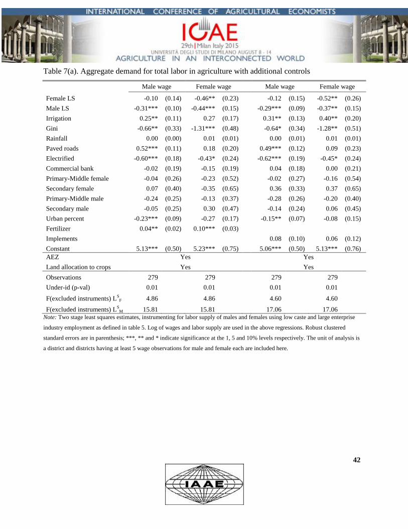
42

Table 7(a). Aggregate demand for total labor in agriculture with additional controls

Male wage Female wage

Male wage Female wage

Female LS -0.10 (0.14) -0.46** (0.23)

-0.12 (0.15) -0.52** (0.26)

Male LS -0.31*** (0.10) -0.44*** (0.15)

-0.29*** (0.09) -0.37** (0.15)

Irrigation 0.25** (0.11) 0.27 (0.17)

0.31** (0.13) 0.40** (0.20)

Gini -0.66** (0.33) -1.31*** (0.48)

-0.64* (0.34) -1.28** (0.51)

Rainfall 0.00 (0.00) 0.01 (0.01)

0.00 (0.01) 0.01 (0.01)

Paved roads 0.52*** (0.11) 0.18 (0.20)

0.49*** (0.12) 0.09 (0.23)

Electrified -0.60*** (0.18) -0.43* (0.24)

-0.62*** (0.19) -0.45* (0.24)

Commercial bank -0.02 (0.19) -0.15 (0.19)

0.04 (0.18) 0.00 (0.21)

Primary-Middle female -0.04 (0.26) -0.23 (0.52)

-0.02 (0.27) -0.16 (0.54)

Secondary female 0.07 (0.40) -0.35 (0.65)

0.36 (0.33) 0.37 (0.65)

Primary-Middle male -0.24 (0.25) -0.13 (0.37)

-0.28 (0.26) -0.20 (0.40)

Secondary male -0.05 (0.25) 0.30 (0.47)

-0.14 (0.24) 0.06 (0.45)

Urban percent -0.23*** (0.09) -0.27 (0.17)

-0.15** (0.07) -0.08 (0.15)

Fertilizer 0.04** (0.02) 0.10*** (0.03)

Implements

0.08 (0.10) 0.06 (0.12)

Constant 5.13*** (0.50) 5.23*** (0.75) 5.06*** (0.50) 5.13*** (0.76)

AEZ Yes Yes

Land allocation to crops Yes

Yes

Observations 279

279

279

279

Under-id (p-val) 0.01

0.01

0.01

0.01

F(excluded instruments) L

SF 4.86

4.86

4.60

4.60

F(excluded instruments) L

SM 15.81 15.81 17.06 17.06

Note: Two stage least squares estimates, instrumenting for labor supply of males and females using low caste and large enterprise

industry employment as defined in table 5. Log of wages and labor supply are used in the above regressions. Robust clustered

standard errors are in parenthesis; ***, ** and * indicate significance at the 1, 5 and 10% levels respectively. The unit of analysis is

a district and districts having at least 5 wage observations for male and female each are included here.

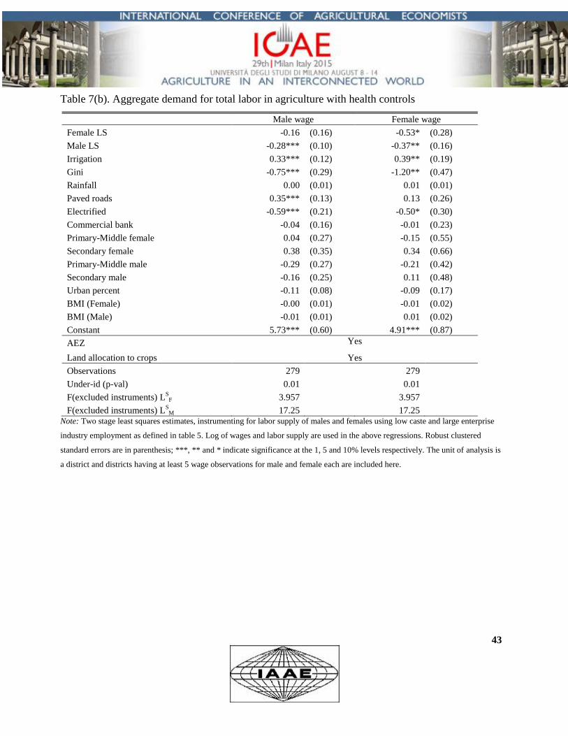
43

Table 7(b). Aggregate demand for total labor in agriculture with health controls

Male wage Female wage

Female LS -0.16 (0.16) -0.53* (0.28)

Male LS -0.28*** (0.10) -0.37** (0.16)

Irrigation 0.33*** (0.12) 0.39** (0.19)

Gini -0.75*** (0.29) -1.20** (0.47)

Rainfall 0.00 (0.01) 0.01 (0.01)

Paved roads 0.35*** (0.13) 0.13 (0.26)

Electrified -0.59*** (0.21) -0.50* (0.30)

Commercial bank -0.04 (0.16) -0.01 (0.23)

Primary-Middle female 0.04 (0.27) -0.15 (0.55)

Secondary female 0.38 (0.35) 0.34 (0.66)

Primary-Middle male -0.29 (0.27) -0.21 (0.42)

Secondary male -0.16 (0.25) 0.11 (0.48)

Urban percent -0.11 (0.08) -0.09 (0.17)

BMI (Female) -0.00 (0.01) -0.01 (0.02)

BMI (Male) -0.01 (0.01) 0.01 (0.02)

Constant 5.73*** (0.60) 4.91*** (0.87)

AEZ Yes

Land allocation to crops Yes

Observations 279

279

Under-id (p-val) 0.01

0.01

F(excluded instruments) LS

F 3.957

3.957

F(excluded instruments) LS

M 17.25 17.25 Note: Two stage least squares estimates, instrumenting for labor supply of males and females using low caste and large enterprise

industry employment as defined in table 5. Log of wages and labor supply are used in the above regressions. Robust clustered

standard errors are in parenthesis; ***, ** and * indicate significance at the 1, 5 and 10% levels respectively. The unit of analysis is

a district and districts having at least 5 wage observations for male and female each are included here.

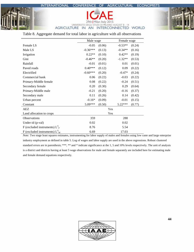
44

Table 8. Aggregate demand for total labor in agriculture with all observations

Male wage Female wage

Female LS -0.05 (0.06) -0.53** (0.24)

Male LS -0.36*** (0.13) -0.34** (0.16)

Irrigation 0.22** (0.10) 0.42** (0.19)

Gini -0.46** (0.20) -1.32** (0.53)

Rainfall -0.01 (0.01) 0.01 (0.01)

Paved roads 0.40*** (0.12) 0.09 (0.22)

Electrified -0.60*** (0.20) -0.47* (0.24)

Commercial bank 0.06 (0.22) -0.03 (0.22)

Primary-Middle female 0.08 (0.22) -0.24 (0.51)

Secondary female 0.20 (0.30) 0.29 (0.64)

Primary-Middle male -0.21 (0.20) -0.16 (0.37)

Secondary male 0.11 (0.26) 0.14 (0.42)

Urban percent -0.16* (0.09) -0.01 (0.15)

Constant 5.09*** (0.50) 5.22*** (0.77)

AEZ Yes

Land allocation to crops Yes

Observations 359

288

Under-id (p-val) 0.02

0.02

F (excluded instruments) LS

F 8.76

5.54

F (excluded instruments) LS

M 6.69 17.03 Note: Two stage least squares estimates, instrumenting for labor supply of males and females using low caste and large enterprise

industry employment as defined in table 5. Log of wages and labor supply are used in the above regressions. Robust clustered

standard errors are in parenthesis; ***, ** and * indicate significance at the 1, 5 and 10% levels respectively. The unit of analysis

is a district and districts having at least 5 wage observations for male and female separately are included here for estimating male

and female demand equations respectively.

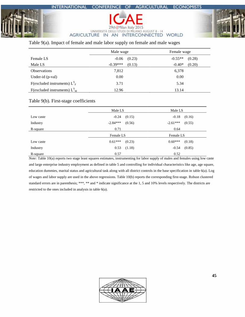
45

Table 9(a). Impact of female and male labor supply on female and male wages

Male wage Female wage

Female LS -0.06 (0.23) -0.55** (0.28)

Male LS -0.39*** (0.13) -0.40* (0.20)

Observations 7,812

6,378

Under-id (p-val) 0.00

0.00

F(excluded instruments) L

SF 3.71

5.34

F(excluded instruments) L

SM 12.96 13.14

Table 9(b). First-stage coefficients

Male LS Male LS

Low caste -0.24 (0.15) -0.18 (0.16)

Industry -2.84*** (0.56) -2.61*** (0.55)

R-square 0.71

0.64

Female LS Female LS

Low caste 0.61*** (0.23) 0.60*** (0.18)

Industry 0.53 (1.18) -0.54 (0.85)

R-square 0.57 0.52

Note: Table 10(a) reports two stage least squares estimates, instrumenting for labor supply of males and females using low caste

and large enterprise industry employment as defined in table 5 and controlling for individual characteristics like age, age square,

education dummies, marital status and agricultural task along with all district controls in the base specification in table 6(a). Log

of wages and labor supply are used in the above regressions. Table 10(b) reports the corresponding first-stage. Robust clustered

standard errors are in parenthesis; ***, ** and * indicate significance at the 1, 5 and 10% levels respectively. The districts are

restricted to the ones included in analysis in table 6(a).

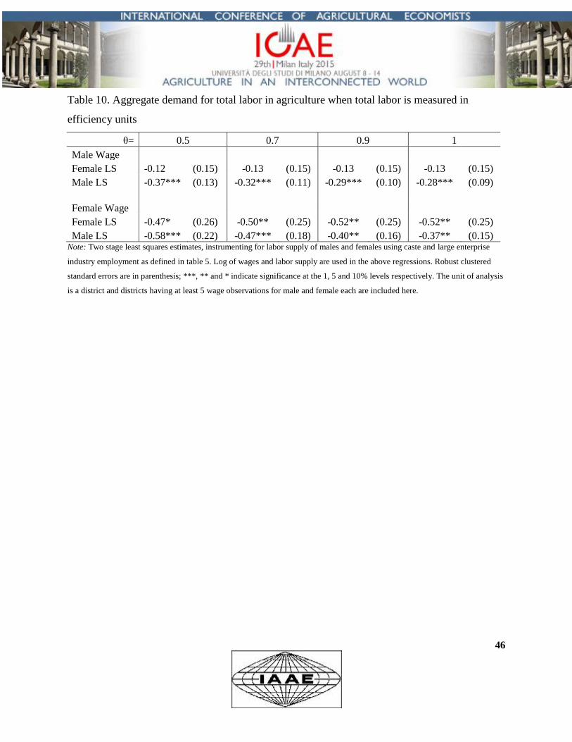
46

Table 10. Aggregate demand for total labor in agriculture when total labor is measured in

efficiency units

θ= 0.5 0.7 0.9 1

Male Wage

Female LS -0.12 (0.15) -0.13 (0.15) -0.13 (0.15) -0.13 (0.15)

Male LS -0.37*** (0.13) -0.32*** (0.11) -0.29*** (0.10) -0.28*** (0.09)

Female Wage

Female LS -0.47* (0.26) -0.50** (0.25) -0.52** (0.25) -0.52** (0.25)

Male LS -0.58*** (0.22) -0.47*** (0.18) -0.40** (0.16) -0.37** (0.15) Note: Two stage least squares estimates, instrumenting for labor supply of males and females using caste and large enterprise

industry employment as defined in table 5. Log of wages and labor supply are used in the above regressions. Robust clustered

standard errors are in parenthesis; ***, ** and * indicate significance at the 1, 5 and 10% levels respectively. The unit of analysis

is a district and districts having at least 5 wage observations for male and female each are included here.

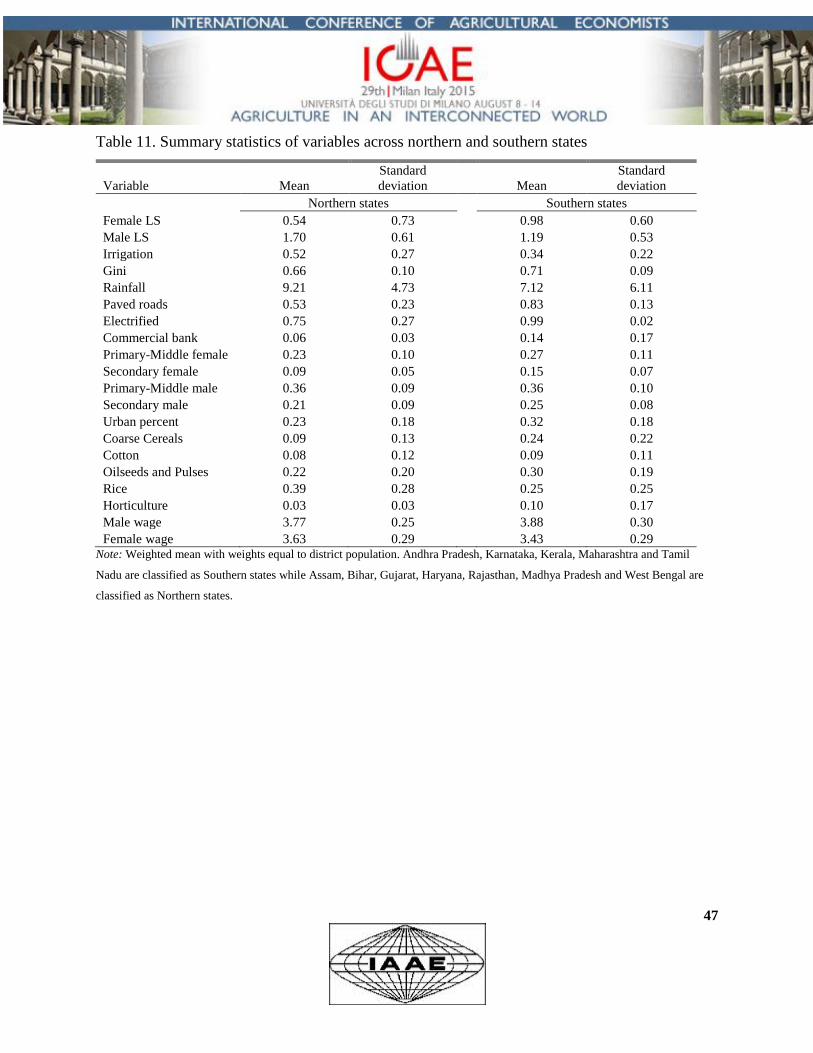
47

Table 11. Summary statistics of variables across northern and southern states

Variable Mean

Standard

deviation Mean

Standard

deviation

Northern states Southern states

Female LS 0.54 0.73

0.98 0.60

Male LS 1.70 0.61

1.19 0.53

Irrigation 0.52 0.27

0.34 0.22

Gini 0.66 0.10

0.71 0.09

Rainfall 9.21 4.73

7.12 6.11

Paved roads 0.53 0.23

0.83 0.13

Electrified 0.75 0.27

0.99 0.02

Commercial bank 0.06 0.03

0.14 0.17

Primary-Middle female 0.23 0.10

0.27 0.11

Secondary female 0.09 0.05

0.15 0.07

Primary-Middle male 0.36 0.09

0.36 0.10

Secondary male 0.21 0.09

0.25 0.08

Urban percent 0.23 0.18

0.32 0.18

Coarse Cereals 0.09 0.13

0.24 0.22

Cotton 0.08 0.12

0.09 0.11

Oilseeds and Pulses 0.22 0.20

0.30 0.19

Rice 0.39 0.28

0.25 0.25

Horticulture 0.03 0.03

0.10 0.17

Male wage 3.77 0.25

3.88 0.30

Female wage 3.63 0.29 3.43 0.29 Note: Weighted mean with weights equal to district population. Andhra Pradesh, Karnataka, Kerala, Maharashtra and Tamil

Nadu are classified as Southern states while Assam, Bihar, Gujarat, Haryana, Rajasthan, Madhya Pradesh and West Bengal are

classified as Northern states.

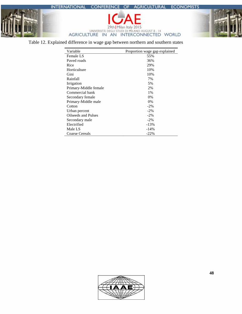
48

Table 12. Explained difference in wage gap between northern and southern states

Variable Proportion wage gap explained

Female LS 55%

Paved roads 36%

Rice 29%

Horticulture 10%

Gini 10%

Rainfall 7%

Irrigation 5%

Primary-Middle female 2%

Commercial bank 1%

Secondary female 0%

Primary-Middle male 0%

Cotton -2%

Urban percent -2%

Oilseeds and Pulses -2%

Secondary male -2%

Electrified -13%

Male LS -14%

Coarse Cereals -22%

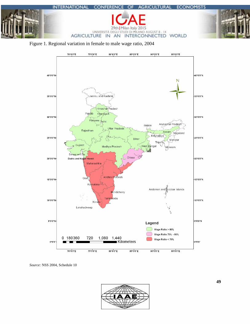
49

Figure 1. Regional variation in female to male wage ratio, 2004

Source: NSS 2004, Schedule 10

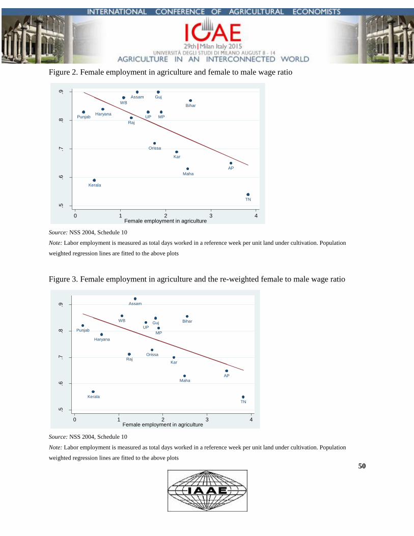
50

Figure 2. Female employment in agriculture and female to male wage ratio

Source: NSS 2004, Schedule 10

Note: Labor employment is measured as total days worked in a reference week per unit land under cultivation. Population

weighted regression lines are fitted to the above plots

Figure 3. Female employment in agriculture and the re-weighted female to male wage ratio

Source: NSS 2004, Schedule 10

Note: Labor employment is measured as total days worked in a reference week per unit land under cultivation. Population

weighted regression lines are fitted to the above plots

PunjabHaryana

Raj

UP

Bihar

Assam

WB

Orissa

MP

Guj

Maha

AP

Kar

Kerala

TN

.5.6

.7.8

.9

Wag

e r

atio

0 1 2 3 4Female employment in agriculture

Punjab

Haryana

Raj

UP

Bihar

Assam

WB

Orissa

MP

Guj

MahaAP

Kar

Kerala

TN

.5.6

.7.8

.9

Wag

e r

atio

re

we

igh

ted

0 1 2 3 4Female employment in agriculture

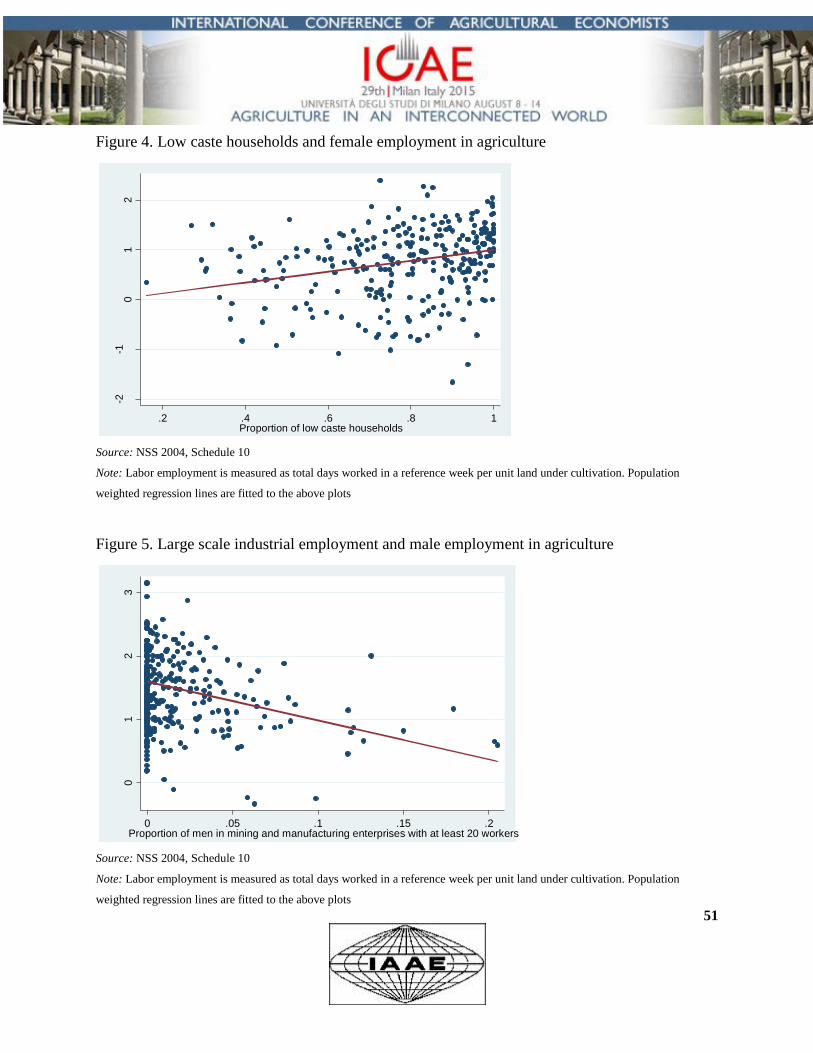
51

Figure 4. Low caste households and female employment in agriculture

Source: NSS 2004, Schedule 10

Note: Labor employment is measured as total days worked in a reference week per unit land under cultivation. Population

weighted regression lines are fitted to the above plots

Figure 5. Large scale industrial employment and male employment in agriculture

Source: NSS 2004, Schedule 10

Note: Labor employment is measured as total days worked in a reference week per unit land under cultivation. Population

weighted regression lines are fitted to the above plots

-2-1

01

2

Log

fem

ale

em

plo

ym

en

t in

agri

cu

lture

.2 .4 .6 .8 1Proportion of low caste households

01

23

Log

ma

le e

mplo

ym

en

t in

agri

culture

0 .05 .1 .15 .2Proportion of men in mining and manufacturing enterprises with at least 20 workers

52

Appendix A.1: Data sources

Wages, Labor supply, Gini, Education, Low caste, Large scale non-farm employment in

manufacturing and mining units- National Sample survey 2004-05

Irrigation, Land under cultivation- Land Use Statistics 2004-05

Fertilizer- Fertilizer Association of India 2004-05

Crop composition- Area, Production and Yield statistics 2004-05

Rainfall- India Water Portal 2004-05(data originally collected by Indian Meteorological

Department)

Agro Ecological Zones- Compiled by Richard Palmer-Jones and Kunal Sen

Urban, Paved roads, Electrified and Commercial banks- Census of India 2001, Village directory

Implements- Livestock Census 2003