Embed Size (px)
Citation preview

Casualty Actuarial Society E-Forum, Spring 2016
Casualty Actuarial Society E-Forum, Spring 2016 i
The CAS E-Forum, Spring 2016
The Spring 2016 edition of the CAS E-Forum is a cooperative effort between the CAS E-Forum Committee and various other CAS committees, task forces, or working parties. This E-Forum contains Report 12 of the CAS Risk-Based Capital Dependencies and Calibration Working Party (Reports 1 and 2 are posted in E-Forum Winter 2012-Volume 1; Reports 3 and 4 in E-Forum Fall 2012-Volume 2; Report 5 in E-Forum Summer 2012; Report 6 in E-Forum Fall 2013; Report 7 in E-Forum Fall 2013; Report 8 in E-Forum Spring 2014; Report 9 in E-Forum Fall 2014-Volume 2; Report 10 in E-Forum Winter 2015; and Report 11 in E-Forum Winter 2016. This E-Forum also contains one independent research paper and one ratemaking call paper, which was created in response to a call for papers on ratemaking issued by the CAS Committee on Ratemaking.
Risk-Based Capital Dependencies and Calibration Research Working Party Allan M. Kaufman, Chairperson
Karen H. Adams Emmanuel Theodore Bardis Jess B. Broussard Robert P. Butsic Pablo Castets Damon Chom, Actuarial
Student Joseph F. Cofield Jose R. Couret Orla Donnelly Chris Dougherty Nicole Elliott Brian A. Fannin Sholom Feldblum Kendra Felisky Dennis A. Franciskovich Timothy Gault
Dean Guo, Actuarial Student Jed Nathaniel Isaman Shira L. Jacobson Shiwen Jiang James Kahn Alex Krutov Terry T. Kuruvilla Apundeep Singh Lamba Giuseppe F. LePera Zhe Robin Li Lily (Manjuan) Liang Thomas Toong-Chiang Loy Eduardo P. Marchena Mark McCluskey James P. McNichols Glenn G. Meyers Daniel M. Murphy
Douglas Robert Nation G. Chris Nyce Jeffrey J. Pfluger Yi Pu Ashley Arlene Reller David A. Rosenzweig David L. Ruhm Andrew Jon Staudt Timothy Delmar Sweetser Anna Marie Wetterhus Jennifer X. Wu Jianwei Xie Ji Yao Linda Zhang Christina Tieyan Zhou Karen Sonnet, Staff Liaison
Committee on Ratemaking Morgan Haire Bugbee, Chairperson Sandra J. Callanan, Vice Chairperson
LeRoy A. Boison William M. Carpenter James Chang Sa Chen Donald L. Closter Christopher L. Cooksey Sean R. Devlin John S. Ewert
Greg Frankowiak Serhat Guven Duk Inn Kim Dennis L. Lange Ronald S. Lettofsky Lu Li Yuan-Chen Liao Shan Lin
Robert W. Matthews Gregory F. McNulty Jane C. Taylor Lingang Zhang Karen Sonnet, Staff Liaison
Casualty Actuarial Society E-Forum, Spring 2016 ii
CAS E-Forum, Spring 2016
Table of Contents
CAS Research Working Party Report
Insurance Risk-Based Capital with a Multi-Period Time Horizon Report 12 of the CAS Risk-Based Capital (RBC) Research Working Parties Issued by the RBC Dependencies and Calibration Working Party (DCWP) ............ 1-85
CAS Ratemaking Call Paper
Pitfalls of Predictive Modeling Ira Robbin, Ph.D., ACAS ................................................................................................. 1-21
Independent Research
A Practical Introduction to Machine Learning for Actuaries Alan Chalk, FIA, MSc, and Conan McMurtrie, MSc .................................................... 1-30

Casualty Actuarial Society E-Forum, Spring 2016 iii
E-Forum Committee Dennis L. Lange, Chairperson
Cara Blank Mei-Hsuan Chao Mark A. Florenz
Mark M. Goldburd Karl Goring
Derek A. Jones Donna Royston, Staff Liaison/Staff Editor
Bryant Russell Shayan Sen Rial Simons
Elizabeth A. Smith, Staff Liaison/Staff Editor John Sopkowicz
Zongli Sun Betty-Jo Walke
Qing Janet Wang Windrie Wong Yingjie Zhang
For information on submitting a paper to the E-Forum, visit http://www.casact.org/pubs/forum/.
Casualty Actuarial Society E-Forum, Spring 2016 1
Insurance Risk-Based Capital with a Multi-Period Time Horizon
Report 12 of the CAS Risk-Based Capital (RBC) Research Working Parties Issued by the RBC Dependencies and Calibration Subcommittee
Robert P. Butsic ____________________________________________________________________________________________
Abstract: There are two competing views on how to determine capital for an insurer whose loss liabilities extend for several time periods until settlement. The first focuses on the immediate period (usually one-year) and the second uses the runoff (until ultimate loss payment) time frame; each method will generally produce different amounts of required capital. Using economic principles, this study reconciles the two views and provides a general framework for determining capital for multiple periods.
For an insurer whose liabilities and corresponding assets extend over a single time period, Butsic [2013] determined the optimal capital level by maximizing the value of the insurance to the policyholder, while providing a fair return to the insurer’s owners. This paper extends those results to determine optimal capital when liabilities last for several time periods until settlement. Given the optimal capital for one period, the analysis applies backward induction to find optimal capital for successively longer time frames.
A key element in this approach is the stochastic process for loss development; another is the choice of capital funding strategy, which must respond to the evolving loss estimate. In addition to the variables that affect the optimal one-period capital amount (such as the loss volatility, frictional cost of capital and the policyholder risk preferences), in this paper I show that the horizon length, the capitalization interval (time span between potential capital flows), and the policy term will influence the optimal capital for multiple time periods. Institutional and market factors, such as the conservatorship process for insolvent insurers and the cost of raising external capital, also play a major role and are incorporated into the model.
Results show that the optimal capital depends on both the annual and the ultimate loss volatility. Consequently, more total capital (ownership plus policyholder-supplied capital) is required as the time horizon increases; however, optimal ownership capital may decrease as the time horizon lengthens due to the policyholder-supplied capital, which includes premium components for risk margins and income taxes. Also, less capital is needed if capital flows can occur frequently and/or if the policy term is shorter. Insurers that are able to more readily raise capital externally will need to carry less of it.
The model is extended to develop asset risk capital and incorporate features, such as present value and risk margins, that are necessary for practical applications. Although the primary focus is property-casualty insurance, the method can be extended to life and health insurance. In particular, the approach used to determine capital required for multi-period asset risk will apply to these firms.
The resulting optimal capital for insurers can form the basis for pricing, corporate governance and regulatory applications.
Keywords: Backward induction, capital strategy, capitalization interval, certainty-equivalent loss,
conservatorship, exponential utility, fair-value accounting, policy term, risk margin, stochastic loss process, technical insolvency, time horizon
____________________________________________________________________________________________
1. INTRODUCTION AND SUMMARY
There is a considerable body of literature on how to determine the appropriate risk-based capital
for an insurance firm. Generally, the analysis applies a particular risk measure (such as VaR or
expected policyholder deficit), calibrated to a specific valuation level (e.g., VaR at 99.5%) to

Insurance Risk-Based Capital with a Multi-Period Time Horizon
Casualty Actuarial Society E-Forum, Spring 2016 2
determine the proper amount of capital. However, most of the commonly-used risk measures apply
most readily to short-duration risks, for example, property insurance, where the liabilities are settled
within a single time period. Application of these methods is more problematic when addressing
long-term insurance claims, such as liability, workers compensation and life insurance.
How to treat long-term, or multi-period, liabilities and assets is the subject of much debate in the
actuarial and insurance finance literature. For a good, practically-oriented discussion of this topic,
see Lowe et al [2011]. Essentially there are two camps: one side advocates using an annual1 (one-
period) time horizon, wherein the current capital amount must be sufficient to offset default risk
based on loss liability and asset values over the upcoming period, usually one year. The other side
argues that the current capital must offset the default over the entire duration (the runoff horizon)
required to settle the liability. Essentially, the issue is whether capital depends on the loss volatility
only for the upcoming year, or the ultimate loss volatility. This controversy has gained momentum
with the impending implementation of the Solvency II risk-based capital methodology, which uses
an annual (single-period) time horizon.2
As shown in the subsequent analysis, the problem may be solved by extending the one-period
model to a longer time frame. I have used the concept of an optimal capital strategy to determine the
appropriate capital amount for the current period, which is the first period of a multi-period liability.
For a one-period liability, there is a theoretically optimal amount of capital that depends on the
insurer’s cost of holding capital and the nature of the policyholders’ risk aversion. These results are
derived in An Economic Basis for Property-Casualty Insurance Risk-Based Capital Measurement (Butsic
[2013]), which develops the appropriate risk measure (adjusted ruin, or default probability) and
1 More generally, the period could be shorter than one year, but most applications use the annual time frame. In this paper I use the more general concept of time periods. 2 See the European Parliament Directive [2009]; Article 64.

Insurance Risk-Based Capital with a Multi-Period Time Horizon
Casualty Actuarial Society E-Forum, Spring 2016 3
calibration method (using the frictional cost of capital) for a one-period insurer in an equilibrium
insurance setting. The analysis here can be considered as an extension to this paper which, for
reference, I shorten to EBRM.
With multi-period risks, we can use the same fundamental assumptions that drive optimal capital
for a single period. The main point is that, as in a one-period model, the optimal capital over several
periods depends on the balance between capital costs and the amount that the policyholders are
willing to pay to reduce their perceived value of default.
Capital in this paper is defined in the general accounting sense as the difference between assets
and liabilities. For practical applications, capital will need to be defined according to a standard
accounting convention such as IFRS,3 U.S. statutory accounting or the accounting used in Solvency
II.
Although the analysis is geared toward producing optimal capital for property-casualty insurance
losses, the methodology also applies to long-term asset risk and life insurance (see sections 8 and 9).
1.1 Summary The main result of this paper is that the optimal capital for an insurer with multi-period losses
depends on both the volatility of losses for the current year and the volatility of the ultimate loss
value. The ultimate loss volatility is a factor because, when an insurer becomes insolvent, it generally
enters conservatorship and the losses will develop further, as if the insurer had remained solvent.
This further development depends on the ultimate loss volatility. As long as there is volatility for
remaining loss development, the optimal total capital (defined as ownership plus policyholder-
supplied capital) increases as the time horizon lengthens, but at a decreasing rate. However, because
3 In IFRS (International Financial Reporting Standards) and Solvency II accounting, the value of unpaid claim liabilities is treated as the best estimate of the unpaid claims plus a risk margin. Sections 2-7 treat liabilities as the best estimate of unpaid claims. The effect of risk margins is discussed in Section 8.

Insurance Risk-Based Capital with a Multi-Period Time Horizon
Casualty Actuarial Society E-Forum, Spring 2016 4
policyholder-supplied capital (needed to pay future capital costs and the risk margin) is included in
premiums, and these also increase with loss volatility, the optimal amount of ownership capital may
decrease if the time horizon is long enough. The ownership capital (e.g., statutory surplus or
shareholder equity on an accounting basis) is normally the relevant quantity used for risk-based
capital analysis.
For a multiple-period time horizon, the amount of optimal capital depends on the same variables
as for an insurer with a single-period horizon: the frictional cost of holding capital (primarily the cost
of double-taxation), the degree of policyholder risk aversion, loss/asset volatility and guaranty fund
participation. However, with multiple periods, optimal capital also depends on
1. The underlying stochastic process for loss development; the horizon length is also a random variable.
2. What happens to unpaid losses when an insolvency occurs? In particular, conservatorship for an insolvent insurer has a strong effect.
3. The capital strategy used by the insurer. The ability to add capital when needed is particularly important.
4. The cost of raising external capital. In the case of some mutual insurers or privately-held insurers, the limitation on the ability to raise capital is a key factor.
5. The length of time between capital flows. The shorter this time frame, the less capital is needed.
6. The policy term. More capital is needed for a longer term, since if default occurs early in the term, the remaining coverage must be repurchased.
Also, the optimal capital depends on two factors important for multi-period risk that are not
modeled (for simplicity) in EBRM:
1. The interest rate. As the interest rate increases, less capital is necessary to mitigate default that will occur in the future.
2. The risk margin (or market price of risk) embedded in the premium. This amount acts as policyholder-supplied capital and reduces the amount of ownership capital needed.
As identified in items 3 through 5, optimal capital depends on the insurer’s ability to raise capital
and the cost of doing so. A lower cost of raising capital and/or better ability to raise capital will

Insurance Risk-Based Capital with a Multi-Period Time Horizon
Casualty Actuarial Society E-Forum, Spring 2016 5
imply a lower amount of optimal capital. For most insurers, the best feasible strategy is to add capital
when it will improve policyholder welfare, and withdraw capital otherwise. This strategy of adding
capital where appropriate (called AC) means that capital is added only if the insurer remains solvent.
An alternative strategy (full recapitalization, or FR), adds capital even when the insurer is insolvent.
Under FR, only the current-period loss volatility is considered and thus is consistent with the
Solvency II risk-based capital methodology.4 However, the FR strategy is not feasible, so the
Solvency II method can understate risk-based capital for long-horizon losses.
The optimal capital for an insurer with asset risk is determined by combining the asset risk with
the loss risk, and getting the joint capital for both. The implied amount of asset-risk capital is
obtained by subtracting the loss-only optimal capital from the joint capital. If the asset risk is low, it
is possible that the optimal capital for the combined risks is lower than that for the loss-only risk.
Two factors tend to reduce the optimal implied asset-risk capital for long time horizons, compared
to the loss-only risk capital. First, when an insurer becomes technically insolvent, asset risk is
virtually eliminated, as a consequence of entering conservatorship (where the insurer’s investments
are replaced with low-risk securities). Second, the positive expected return from risky assets acts as
additional capital. As with losses, the optimal asset-risk total capital increases with the time horizon
length.
1.2 Outline The remainder of the paper is summarized thusly:
4 The Solvency II approach to risk margins and capital adequacy can be interpreted as assuming that recapitalization is always possible. Note however, that the Solvency II approach includes liability risk margins that increase the amount of assets required of the insurer. These assets increase with the horizon length. The additional (policyholder-supplied) capital from those assets depends on the ultimate loss volatility, so that the Solvency II method does not rely solely on the current-period loss volatility. Other than the risk margin issue, I do not compare the Solvency II assumptions to those of the models developed in this paper.

Insurance Risk-Based Capital with a Multi-Period Time Horizon
Casualty Actuarial Society E-Forum, Spring 2016 6
Key Results from the One-Period Model (Section 2)
Section 2 summarizes the results for a one-period model, showing how the cost of holding
capital and the policyholder risk preferences will provide an optimal capital amount. Coupled with
the insurer’s capital strategy, the one-period optimal capital amounts will generate optimal capital for
longer-duration losses spanning multiple periods.
Multi-Period Model Issues (Section 3)
Section 3 introduces issues presented in a multi-period model that are not applicable to the one-
period case. These issues are explored further in subsequent sections. A key concept is the stochastic
loss development process, wherein the estimate of the ultimate loss fluctuates randomly from period
to period, with the current estimate being the mean of the ultimate loss distribution; this process
determines expected default values in future periods. Another important issue is the impact on
assets and loss liabilities following technical insolvency, where a regulator forces an insurer to cease
operations when its assets are less than its liabilities; in this case, losses continue to develop after the
insurer has defaulted. I describe capital funding strategies, which are necessary to address the period-
to-period loss evolution. This section also discusses the distinction between ownership capital and
policyholder-supplied capital; this issue may not be relevant in a one-period model.
Basic Multi-period Model (Section 4)
Section 4 presents a basic model of an insurer with multiple-period losses for liability insurance.
First, I summarize the assumptions underlying a one-period model and add those necessary for a
multi-period model. Then I describe characteristics of the loss development stochastic process,
including a parallel certainty-equivalent process needed to value the default from the policyholders’
perspective. Third, I specify a premium model, which allows the calculation of the value of the
insurance contract to both policyholders and the insurer, and thus the optimum capital amount for

Insurance Risk-Based Capital with a Multi-Period Time Horizon
Casualty Actuarial Society E-Forum, Spring 2016 7
both parties. Fourth, I examine the distinction between ownership capital and total capital, which
also includes policyholder-supplied capital.5 Fifth, I discuss capital funding strategies, where insurers
attempt to add or withdraw capital to maintain an optimal position over time; the strategies vary
according to efficiency (value to policyholders) and feasibility. Finally, I show that the most efficient
feasible strategy is where capital is added if the insurer remains solvent; this is denoted as AC.
Optimal Two-period Capital (Section 5)
Section 5 determines the optimal capital for a two-period model under the AC strategy. Here I
evaluate the certainty-equivalent value of default under technical insolvency, which is a key
component of the analysis. This section introduces a stochastic loss process with normally-
distributed incremental development, used in subsequent sections to illustrate optimal capital
calculation. Next, the AC model is enhanced to incorporate an additional cost of providing capital
from external sources. Finally, I analyze the how optimal capital can be determined for an insurer
with limited ability to raise external capital, such as a mutual insurer.
Optimal Capital for More Than Two Periods (Section 6)
Section 6 extends the two-period model to multiple periods using backward induction. This
procedure provides optimal initial capital for the various capital strategies.
Capitalization Interval (Section 7)
Section 7 examines how optimal insurer capital depends on the capitalization interval, or the time
span required to add capital from external sources. This interval determines the period length for a
multi-period model. Section 7 also shows how the policy term affects optimal capital.
Extensions to the Multi-period Model (Section 8)
5 For shareholder-owned insurers, policyholder-supplied capital includes the premium components of risk margins and provision for income taxes. In addition to these funds, policyholders of mutual insurers provide ownership capital in their premiums.

Insurance Risk-Based Capital with a Multi-Period Time Horizon
Casualty Actuarial Society E-Forum, Spring 2016 8
Section 8 extends the basic multi-period model to include features necessary for a practical
application. I apply a stochastic horizon, where the loss development continues for a random length
of time. Also, the analysis shows the effect of using present value and risk margins. The section
concludes with a brief discussion of applying the methodology to life and health insurance.
Multi-Period Asset Risk (Section 9)
Section 9 determines optimal capital for asset risk by extending the loss model to a joint loss and
asset model. The joint model is simplified by using an augmented loss variable, which incorporates
the asset risk and return into a loss-only model.
Conclusion (Section 10)
Section 10 concludes the paper.
Other Material
Appendix A through Appendix D contain detailed numerical examples that illustrate key
concepts and provide additional mathematical development. The References provide sources for
footnoted information. To assist in following the analysis, the Glossary explains the mathematical
notation and abbreviations used in the paper. The final section is a Biography of the Author.
2. KEY RESULTS FROM THE ONE-PERIOD MODEL
This discussion briefly shows how optimum capital is determined in a one-period model. More
details can be found in EBRM.
2.1 Certainty-Equivalent Losses Since a policyholder is presumed to be risk-averse, the perceived value of each possible loss, or
claim, amount is different from the nominal value. For a policyholder facing a random loss, the
certainty-equivalent (CE) value of the loss is the certain amount the policyholder is willing to pay in
Insurance Risk-Based Capital with a Multi-Period Time Horizon
Casualty Actuarial Society E-Forum, Spring 2016 9
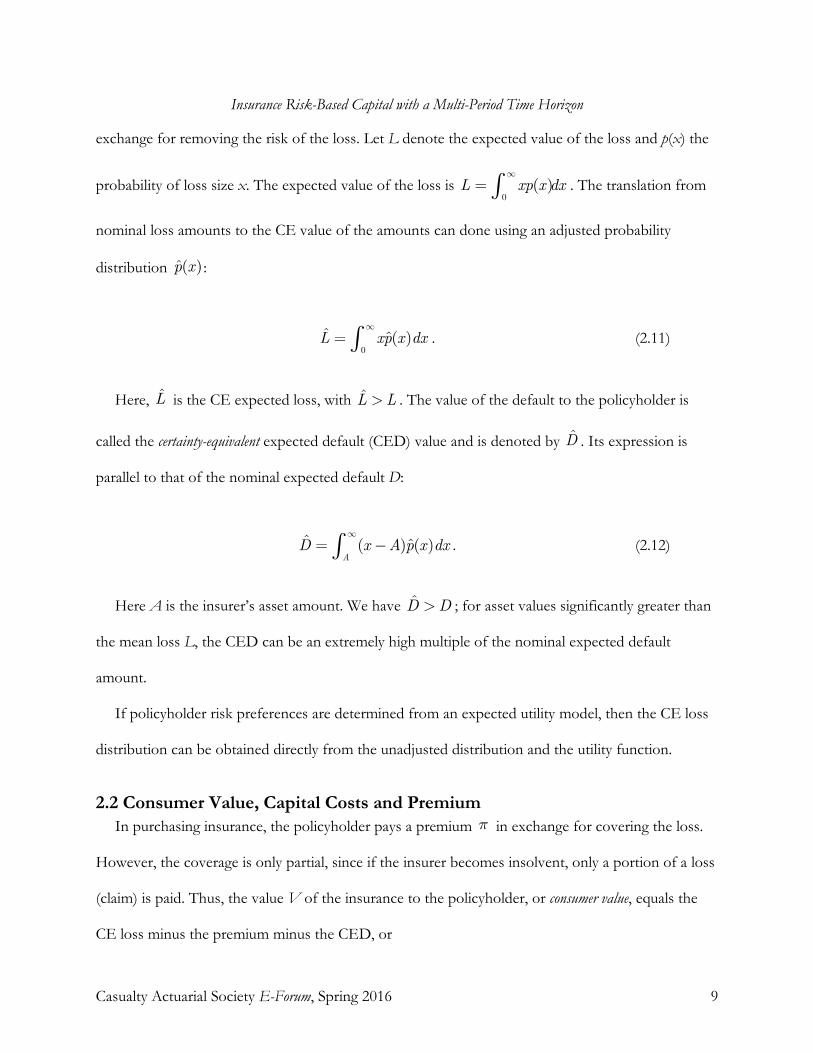
exchange for removing the risk of the loss. Let L denote the expected value of the loss and p(x) the
probability of loss size x. The expected value of the loss is . The translation from
nominal loss amounts to the CE value of the amounts can done using an adjusted probability
distribution :
. (2.11)
Here, is the CE expected loss, with . The value of the default to the policyholder is
called the certainty-equivalent expected default (CED) value and is denoted by . Its expression is
parallel to that of the nominal expected default D:
. (2.12)
Here A is the insurer’s asset amount. We have ; for asset values significantly greater than
the mean loss L, the CED can be an extremely high multiple of the nominal expected default
amount.
If policyholder risk preferences are determined from an expected utility model, then the CE loss
distribution can be obtained directly from the unadjusted distribution and the utility function.
2.2 Consumer Value, Capital Costs and Premium In purchasing insurance, the policyholder pays a premium in exchange for covering the loss.
However, the coverage is only partial, since if the insurer becomes insolvent, only a portion of a loss
(claim) is paid. Thus, the value V of the insurance to the policyholder, or consumer value, equals the
CE loss minus the premium minus the CED, or

Insurance Risk-Based Capital with a Multi-Period Time Horizon
Casualty Actuarial Society E-Forum, Spring 2016 10
. (2.21)
If V > 0, then the policyholder will buy the insurance.
In the basic model described in EBRM (see the assumptions in Section 4) the only costs to the
insurer are the loss and the frictional cost of capital (FCC), denoted by z. The FCC is primarily
income taxes, but may include principal-agent, regulatory restriction or other costs. Assuming that
the capital cost is strictly proportional to the capital amount C, the premium is
. (2.22)
Since adding capital reduces the CED but increases premium (through a higher capital cost),
there generally will be an optimal level of capital that maximizes V and therefore provides the
greatest policyholder welfare. By taking the derivative of V with respect to the asset amount A, we
get the requirement for optimal assets, and therefore optimal capital:
. (2.23)
Here is the default, or ruin, probability under the adjusted probability ; it equals the
negative derivative of with respect to A. This result assumes that the premium is not reduced by
the amount of expected default; if so, then equation 2.23 is an approximation.
Meanwhile, the insurer’s owners are fairly compensated for the capital cost through the zC
component of the premium, so their welfare is also optimized. Since policyholder and shareholder
welfare are both maximized, this theoretical optimal capital level can form the basis for pricing,
regulation and internal insurer governance.
Notice that if there were no prospect of the insurer’s default and the cost of capital were zero,
Insurance Risk-Based Capital with a Multi-Period Time Horizon
Casualty Actuarial Society E-Forum, Spring 2016 11
the consumer value of insurance would be the CE expected loss minus the nominal expected loss, or
. Call this amount the risk value. It is the maximum possible value that the policyholder could
obtain by purchasing insurance. In the basic model, the prospect of default introduces the frictional
capital cost and the CE expected default as elements that are subtracted from the risk value to
produce the net consumer value. A useful term for the sum of these two amounts is the solvency cost.
Since the risk value is not a function of the insurer’s assets (the basic model assumes riskless assets;
risky assets are analyzed in section 9), minimizing the solvency cost is equivalent to maximizing the
consumer value.
3. MULTI-PERIOD MODEL ISSUES
Determining optimal capital for multiple periods presents several challenges not evident in the
one-period situation. These issues are introduced below and are addressed in greater depth in
sections 4 through 9.
3.1 Stochastic Loss Development In the one-period case, the loss is initially unknown, but its value is revealed at the end of the
period. For multiple periods, the loss value may remain unknown for several periods. Consequently,
in order to establish the necessary capital amount for each period (using the accounting identity that
capital equals assets minus liabilities), we need to estimate the ultimate loss; this assessment is known
as the loss reserve. The reserve estimate will vary randomly from period to period until the loss is
finally settled. The stochastic reserve estimates will form the basis for a dynamic capital strategy.
3.2 Default Definition and Liquidation Management In a multi-period model, the loss reserve values are estimates of the ultimate unpaid loss liability. If
the estimated loss exceeds the value of assets at the end of a period, the insurer is deemed to be
Insurance Risk-Based Capital with a Multi-Period Time Horizon
Casualty Actuarial Society E-Forum, Spring 2016 12
technically insolvent. The insolvency is “technical” because it is possible that the reserve may
subsequently develop downward and there is ultimately no default. If the insurer adds sufficient
capital to regain solvency, then there is the further possibility that the insurer may yet again become
insolvent in future periods. Thus, multiple insolvencies are theoretically possible for a recapitalized
individual insurer that emerges from an initial technical insolvency.
Generally, when an insurer becomes technically insolvent, regulators transfer its assets and
liabilities to a conservator, or receiver, who manages them in the interests of the policyholders. This
usually means that the assets are invested conservatively in low-risk securities6 and when claims are
paid, each policyholder gets the same pro-rata share of the assets according to their claim amounts.
There are several important consequences to receivership. First, the liabilities remain “alive” and
are allowed to develop further. Second, there is no source of additional capital to mitigate the
ultimate default amount (however, no capital can be withdrawn either, unless the assets become
significantly larger than the liabilities). Third, the conservative asset portfolio will most likely have a
significantly reduced asset risk compared to that of the insurer prior to conservatorship. These
features profoundly affect the multi-period capital analysis, as shown in the subsequent sections.
3.3 Dynamic Capital Strategy In a one-period model the capital is determined once, at the beginning of the period. In a multi-
period model, capital is likewise determined initially, but it also must be determined again at the
beginning of each subsequent period. In order to optimize the amount of capital used, the capital-
setting process will require a predetermined strategy. This strategy is dynamic: the subsequent capital
6 For example, the state of California uses an investment pool for its domiciled insurers in liquidation. The pool contains only investment grade fixed income securities with duration less than 3 years (see California Liquidation Office 2014 Annual Report). New York is more conservative: funds are held in short-term mutual funds containing only U.S. Treasury or agency securities with maturities under 5 years (see New York Liquidation Bureau 2014 Annual Report).

Insurance Risk-Based Capital with a Multi-Period Time Horizon
Casualty Actuarial Society E-Forum, Spring 2016 13
amounts will depend on the values of the assets and of the insurer liabilities as they evolve. Even
though the capital strategy is dynamic, there will be an optimal starting capital amount. Also, for
each strategy, viewed at the beginning of the first period, there will be a distinct expected amount of
capital at the beginning of each subsequent period.
3.4 Capital Funding Since there is a cost to the insurer for holding capital, the insurer must be compensated for this
cost. This cost is included in the premium. In a one-period model, the premium is paid up front and
the loss is paid at the end of the period; there is no need to consider subsequent capital
contributions. In a multi-period model, the liability estimate may increase over time, leaving the
insurer’s assets insufficient to adequately protect against insolvency. In such an event, the
policyholders will be better off if the insurer’s shareholders contribute additional capital. However,
the insurer will be worse off due to the added capital cost. Nevertheless, if the premium includes the
cost of additional capital funding, consistent with a particular funding strategy, it is economically
practical for the insurer to make the capital contribution. Conversely, if the loss reserve decreases, it
may be mutually beneficial for the insurer to remove some capital, consistent with the capital
funding strategy.
For an ongoing insurer, there is a strong incentive to add capital as needed, since failure to do so
may jeopardize the ability to acquire new business or renew existing policies. However, if technical
insolvency occurs, it may not be feasible for the shareholders to add capital, since the prospect of a
fair return on the capital may be dim. Thus, there are some limitations on capital additions. For a
true runoff insurer, however, there is no incentive to add capital, so capital can only be withdrawn
(which may occur if allowed by regulators).

Insurance Risk-Based Capital with a Multi-Period Time Horizon
Casualty Actuarial Society E-Forum, Spring 2016 14
3.5 Capital Definition In a multi-period model, the premium will include the expected frictional cost of capital for all
future periods. However, at the end of the first period, only the first-period capital cost is expended
for the multi-period model, and so the balance becomes an asset that is available to pay losses. This
premium component thus can be considered as policyholder-supplied capital, since it increases the asset
amount and serves to mitigate default in exactly the same way as the owner-supplied capital in the
one-period model. Similarly, if the premium contains a provision for the insurer’s cost of bearing
risk (a risk margin), that amount will also function as capital. Section 4.4 discusses the distinction
between ownership capital and policyholder-supplied capital. Section 8.3 develops optimal capital
with a risk margin.
4. BASIC MULTI-PERIOD MODEL
This section extends the one-period model to N periods and discusses some important
differences between the two cases. The basic model developed here is designed to contain a minimal
set of features that directly illustrates the optimal capital calculation. Other features, which may be
necessary for practical applications, are discussed in sections 5 through 8.
The basic multi-period model follows a specific cohort of policies insuring losses that occur at
the start of the first period and which are settled at the end of the Nth period. The model assumes
that the insurer is ongoing, so that other similar policies are added at the beginning of the other
periods. The basic model does not track these other policies; however, the prospect of profit from
the additional insurance provides an incentive to add more capital to support the basic model
cohort, if necessary.
4.1. Model Description and Assumptions I start by adopting the basic assumptions of the one-period model, as developed in EBRM, and
Insurance Risk-Based Capital with a Multi-Period Time Horizon
Casualty Actuarial Society E-Forum, Spring 2016 15
modifying some of them to fit the requirements of the multi-period model, as indicated below.
(1) Policyholders are risk averse with homogeneous risk preferences and their losses have the same probability distribution. Thus, the certainty-equivalent values of losses and default amounts are identical for each policyholder.
(2) There are no expenses (administrative costs, commissions, etc.). The only relevant costs are the frictional capital costs and the losses. These costs determine the premium.
(3) The cash flows for premium and the initial capital contribution occur at the beginning of the first period. The frictional capital cost is expended at the end of each period (before the loss is paid).7 The entire loss is paid at the end of the last period. Other capital contributions or withdrawals may occur at the beginning of each subsequent period, depending on the insurer’s capital strategy.
(4) The interest rate is zero. This simplification makes the exposition less cluttered (since the nominal values equal present values) and does not affect the key results. Section 8.2 provides results with a positive interest rate.
(5) Losses have no correlation with economic factors and consequently have no risk margin. Thus, since the investment return is also zero, the expected return on owner-supplied capital is also zero.8 Section 8.3 analyzes results with a risk margin.
(6) The frictional capital cost rate is z ≥ 0. It applies to the ownership capital defined in section 4.4.
(7) There is no cost to raising external capital (section 5.4 develops results that include this cost).
(8) There is no guaranty fund or other secondary source of default protection for policyholders. The only insolvency protection for policyholders is the assets held by the insurer.
(9) Capital adequacy is assessed only at the end of the period for regulatory purposes. Thus, an insolvency can only occur at the end of a period.
Additionally, we require some assumptions specific to the multi-period case that do not apply to
a one-period model:
7 I chose this assumption to be consistent with the one-period model in EBRM. For the one-period model, this assumption avoids the issue of policyholder-supplied capital vs. ownership capital. If the loss is paid before the capital cost is expended, the optimal capital is determined from , instead of , which is a simpler result that gives approximately the same optimal capital. 8 This is a standard financial economics assumption; with no systematic risk, the required return equals the risk-free rate (which is zero here). There will be a positive expected return if a risk margin (discussed in section 8.3) is included.

Insurance Risk-Based Capital with a Multi-Period Time Horizon
Casualty Actuarial Society E-Forum, Spring 2016 16
(1) The ultimate loss is not necessarily known when the policy is issued, but is definitely known at the end of the Nth period (or sooner). This situation requires an intermediate estimate (the reserve amount) of the ultimate loss at each prior period. The reserve value is unbiased: it equals the expected value of the ultimate loss.
(2) The premium includes the expected FCC, since under a dynamic capital strategy, the capital amounts in future periods will depend on the random loss valuation and thus are also random.
(3) A capital strategy is used, wherein for each possible pair of loss and asset values at the end of each period, the insurer will add or withdraw a predetermined amount of capital.
(4) The policy term is one period. Section 7.4 discusses the case where the term is longer than a single period.
Since the certainty-equivalent value of losses and related expected default amounts are assessed
from the perspective of each individual homogeneous policyholder, we scale the insurer model to
portray each policyholder’s share of the results. Therefore, it is useful to consider the model as
representing an insurer with only a single policyholder.
In the multi-period model with N periods, variables that have a time element are generally
indexed by a subscript denoting a particular period as time moves forward. The index begins at 1 for
the first period and ends at N for the last period. Balance sheet quantities such as assets and capital
are valued at either the beginning or end of the period, depending on the context. For example,
represents capital at the beginning of the first period and denotes the assets for the first period
after the capital cost is expended. For simplicity, I drop the subscript for the first period where the
situation permits.
When developing optimal capital with backward induction (section 6) the index represents the
number of remaining periods: e.g., denotes the initial ownership capital for a three-period model.

Insurance Risk-Based Capital with a Multi-Period Time Horizon
Casualty Actuarial Society E-Forum, Spring 2016 17
Optimal values are represented by an asterisk (e.g., ), certainty-equivalent quantities by a carat
(e.g., ), market values (used in risk margins) by a bar (e.g., ) and random values by a tilde (e.g.,
).
Note that under this simplified model, it is not necessary to distinguish between underwriting risk
(the risk arising from losses on premiums yet unearned) and reserve risk (the risk arising from
development of losses already incurred from prior-written premiums).
4.2 Stochastic Process for Losses To analyze capital requirements, it is useful to categorize property-casualty losses into two
idealized types, which are approximate versions of real-world processes. The first loss type is short-
duration, e.g., property, where losses are settled at the end of the same period as incurred; a loss has
at most a one-period lag between its estimated value when incurred and when ultimately settled. The
second type is long-duration, e.g., liability coverage, where the lag is at least one period; if a loss occurs
in a particular period, its value in a subsequent period will depend on its value in the earlier period.
For analyzing capital under the section 4.1 basic model, short-duration losses are one period,
since the loss value cannot carry over to a subsequent period. Also, the expected value of losses in a
subsequent period is independent of losses occurring in an earlier period. Since the per-policy mean
loss (adjusted for inflation) does not change much over time, property losses generally follow a
stationary stochastic process. With short-duration losses under the basic model considered to be one-
period,9 determining optimal capital is straightforward (see section 2), and so I turn to liability losses.
4.21 Long-Duration Loss Stochastic Process Under a one-period model, the expected loss is L, which is a component of the premium. With a
9 An exception is where the policy term is more than one period. This case is discussed in section 7.4.

Insurance Risk-Based Capital with a Multi-Period Time Horizon
Casualty Actuarial Society E-Forum, Spring 2016 18
multi-period model, we use the same notation for the initial loss estimate. However, there will be
intermediate reserve estimates at the end of the periods 1 through N – 1. The
realized value of the ultimate loss is denoted by . Because we have assumed that the reserve
estimates are unbiased, each reserve value is the mean of the possible values for the next reserve
estimate . In other words, the difference , or the reserve increment, has a zero
mean. The sequence of reserve estimates is a random walk, which is a type of Markov process.10 In a
Markov process the future evolution of the value of a variable does not depend on the history of the
prior values. In other words, conditional on the present reserve value, its future and past are
independent. There cannot be a correlation between successive reserve amounts if the estimates are
unbiased. The normal loss model in section 5.3 is an example of this stochastic process, which is an
additive model since the increments are summed to determine successive values.
An alternative stochastic process that may characterize loss evolution is a multiplicative model.
Here we define , which has a mean of 1 for all t. The product of the multiplicative
random factors and the initial loss estimate L will give the ultimate loss value . The lognormal
loss model in section 5.3 is an example of this stochastic process. Notice that
, which is an additive random walk with a zero mean as described
above.
For simplicity, I assume that the values have the same type of probability distribution (e.g.,
normal) for all time values t. I also assume that the variance of (denoted by ) is constant per
10 See Bharucha-Reid[1960].
Insurance Risk-Based Capital with a Multi-Period Time Horizon
Casualty Actuarial Society E-Forum, Spring 2016 19
period. In practice, this assumption may need to be modified.11 Finally, I assume a similar regularity
for the multiplicative model.
Notice that the variance of the ultimate loss is the sum of the variances of the sequence,
or . There is no covariance between any of the reserve increments due to the memory-less
property of the Markov process (a non-zero correlation would imply that the prior reserve history
could help predict the future reserve values). The variance exists because the flow of
information (positive and negative) regarding the ultimate loss value is random. The subsequent
estimates of ultimate value are determined by information that becomes revealed over time, such as
how many claims have occurred, the nature of the claims, the legal environment, inflation and so
forth.
4.22 Certainty-Equivalent Stochastic Process The certainty-equivalent loss values will evolve according to a stochastic process parallel to that
of the underlying losses. Generally, if the policyholder risk aversion is based on utility theory, the
risk value embedded in the CE losses is approximately proportional12 to the loss variance. The
relationship is exact if the loss values are normally distributed and policyholder risk aversion is
represented by exponential utility. For this additive stochastic process with a constant13 per-period loss
volatility, the CE expected loss at the end of N periods is then
11 This assumption can be modified to provide a specific variance for each period, as will be necessary for practical applications. The actual distribution may vary according to the elapsed claim duration. For example, the long discovery (with claims incurred but not reported) phase for high-deductible claims will imply a low variance for the reserve estimates for the first few years. Scant information regarding the claims arrives over this time span, so there is little basis to revise the initial reserve. 12 See Panjer et al. [1988], page 137. 13 If the loss volatility is not constant, then the term is replaced by , where is the variance of the ith period loss volatility.
Insurance Risk-Based Capital with a Multi-Period Time Horizon
Casualty Actuarial Society E-Forum, Spring 2016 20
, (4.221)
where a is a constant that indicates the degree of risk aversion. Therefore, the CE expected loss
increases each period by the risk value . Since the CE loss mean increases linearly with the
time horizon, we can create a parallel CE stochastic process by satisfying equation 4.221. Appendix
B shows how the N-period CE distribution of losses or assets is determined under the normal-
exponential model and includes a numerical example.
Notice that equation 4.221 represents the CE expected loss value with N periods remaining; as
the loss evolves there will be fewer periods left and the risk value will diminish (it will be zero when
the loss is settled).
Appendix A illustrates a two-period stochastic process with a simple numerical example using a
discrete probability distribution.
4.3 Premium and Balance Sheet Model Following the one-period model, the premium for the multi-period case equals L plus the
expected capital cost. However, the capital for each period after the initial period will be determined
by the evolving loss estimate, so it also will be a random variable. Consequently, the capital cost
component of the premium will be the expected value of the sequence of capital costs. Let C denote
the ownership capital, which is the amount of capital contributed initially (here I drop the subscript 1
for the first period). For a specific capital funding approach, under an N-period model, let be the
capital amount at the beginning of the ith period.
Assume that the frictional capital cost is proportional to the ownership capital (see section 4.4 for a
discussion of capital sources) at the rate z. As shown in EBRM, the double-taxation component of
Insurance Risk-Based Capital with a Multi-Period Time Horizon
Casualty Actuarial Society E-Forum, Spring 2016 21
the capital cost depends solely on the ownership capital amount.14 The expected capital cost for all
periods is then . Accordingly, the fair premium equals
, which has the same form as in the one-period case.
The expected value of the future capital amount or of the capital cost should be calculated using
unadjusted probabilities, since, like the expected return on capital, the frictional capital cost rate z does
not depend on policyholder risk preferences. Also, the insurer is already compensated for the risk it
bears through the risk margin built into the premium. Although the risk margin is zero here in the
basic model, a more general model, such as in section 8.3, will include it.
This premium model forms the basis for pricing methods that use the present value of expected
future costs and whose losses have embedded risk margins (see sections 8.2 and 8.3). The present
value of the expected capital costs is determined by discounting them at a risk-free rate.
When the policies are written, the initial assets equal the owner-contributed capital plus the
premium, or . With a zero interest rate, these assets are cash in the basic
model. The liabilities are the expected losses, the expected capital cost15 and the ownership capital,
which is the residual of assets minus the obligations to other parties. At the end of the first period,
before the loss is paid, the capital cost for that period is expended, leaving the amount of assets
available to pay losses, denoted by A, as
. (4.31)
14 Other frictional capital cost components might depend on total capital or total assets, but since they are likely to be smaller than the double-taxation amount, I have assumed that they also are proportional to the ownership capital. 15 As discussed in EBRM, this amount is primarily an income tax liability.
Insurance Risk-Based Capital with a Multi-Period Time Horizon
Casualty Actuarial Society E-Forum, Spring 2016 22
4.4 Ownership Capital and Total Capital For the basic one-period model, the capital definition is straightforward. At the beginning of the
period, the insurer’s owners supply a capital amount C, and the policyholders supply the premium,
equal to L + zC. Since the capital cost amount zC is expended before the loss is paid, the amount of
assets available to pay the loss is A = L + C.
For a multi-period model, however, the amount available to pay losses after the first period is
greater than L + C by the amount K – zC > 0, which represents the expected capital cost for the
remaining periods. Since this additional amount reduces default in exactly the same way as the
owner-supplied capital, it may be considered as policyholder-supplied capital. Therefore it is useful to
define the total capital as the available assets minus the expected loss, which for the basic multi-period
model is
. (4.41)
Notice that for a one-period model, we have T = C, and for two or more periods,
T > C.
It is important that the ownership capital measurement be consistent with the premium
determination. Here I use fair-value (also known as mark-to market) accounting, where the value of
obligations is the amount they would be worth in a fair market exchange16 and are thus equal to the
fair premium. From equation 4.41 it is simple to determine the fair-value capital from the total
capital and vice-versa. For brevity, I use OC to denote ownership capital.
With a risk margin, discussed in section 8.3, we have a similar situation: the risk margin
16 An important property of fair value accounting is that, if the product is fairly priced (so that its components are priced at market values), there is no profit generated when the product or service is sold. Instead, the profit is earned smoothly over time as the firm’s costs of production or service provision are incurred. For an insurer, this means that the profit will emerge as the risk of loss is borne.

Insurance Risk-Based Capital with a Multi-Period Time Horizon
Casualty Actuarial Society E-Forum, Spring 2016 23
compensates the insurer for bearing risk and is a premium component in addition to the expected
loss. Like the unexpended expected capital cost, it provides additional default protection. However,
in fair-value accounting, the risk margin is not considered as ownership capital.
For the subsequent sections, I present most results using the total capital definition. Where
appropriate, I show the OC for comparison.
4.5 Capital Funding Strategies In order to determine the expected capital cost, we need to know how much capital will be used
for each period. As discussed in section 3.4, the amount will depend on the loss amount at the end
of the prior period: if the amount is large, it may be necessary to add capital; if the amount is small
enough, capital might be withdrawn. Define a capital funding strategy as a set of rules that assigns a
specific amount of capital, called the target amount, to the beginning of each period, corresponding
to each possible loss value at the end of the prior period. Note that there is not necessarily a unique
capital amount for each loss amount, since a range of losses can produce a single capital amount
(such as region 2b in section 5.42).
There are several basic capital funding strategies that an insurer might use. I describe the most
relevant ones below, starting from the least to the most dynamic method.
Fixed Assets (FA): under this approach, the insurer’s owners supply an initial capital amount, with
no subsequent capital flows until the losses are fully settled. Thus, the initial assets remain constant
until the losses are paid. The capital amount will vary over time, since loss estimates will fluctuate
and the capital equals assets minus liabilities. This method is used in Lowe et al. [2011] to determine
capital for a runoff capital model. Although it is viable for a true runoff insurer, it will not be for an
ongoing insurer, whose capital level generally responds to the level of its loss liabilities. For example,
if an insurer’s losses develop favorably, causing its capital amount to increase above a target level

Insurance Risk-Based Capital with a Multi-Period Time Horizon
Casualty Actuarial Society E-Forum, Spring 2016 24
dictated by the strategy, then the insurer will usually reduce its capital amount.
Capital Withdrawal Only (CW): with this strategy, capital is withdrawn if the asset level becomes
high relative to the losses and therefore capital exceeds a particular target amount. A common
method for withdrawing capital is through dividends to shareholders.17 However, no capital is added
if assets become lower than the target level. Except possibly for some mutual insurers, this method
also does not represent actual practice, where, within limits, insurers will add capital if the existing
capital amount is below the target level.
Add Capital if Solvent (AC): here, capital is withdrawn if a particular target level is reached, and
capital is added if assets are below the solvency level. However, if the insurer becomes technically
insolvent, then no capital is added. In this event, the insurer usually is taken over by a conservator.
The incentive for shareholders to fund capital additions comes from the prospect of adding new
business, which is difficult to accomplish without adequate capital. Note that a less restrictive
threshold (where insurers are slightly insolvent) might be used in the event that shareholders
consider the franchise value of the insurer to be valuable enough. However, the results of this
assumption would be analytically similar to using a strict solvency/insolvency threshold. The main
point here is that there is an upper limit to losses beyond which capital is no longer added.
A variation of the AC strategy, discussed in section 5.4, is where there is a cost to raising capital
externally. I have labeled this strategy as ACR.
Full Recapitalization (FR): this approach is similar to AC, but the insurer, even if technically
insolvent, will add sufficient capital to regain the target level. However, in order to provide an
adequate incentive for the shareholders to provide capital if the insurer becomes insolvent, the
17 For a mutual insurer, the dividends will go to policyholders, who are the insurer’s owners and therefore serve as shareholders. A mutual insurer’s dividends can also be used as part of its pricing strategy.

Insurance Risk-Based Capital with a Multi-Period Time Horizon
Casualty Actuarial Society E-Forum, Spring 2016 25
policyholders must accept a cash settlement for their claims; the amount equals the asset value. The
insurer (or a different insurer) then agrees to insure the loss liability again and the policyholders pay
a new premium for the reinstated coverage. The insurer’s owners then provide adequate capital for
the insurance. This transaction, in effect, converts the technical insolvency into a cash or “hard”
insolvency. Thus, it is possible for the insurer to default multiple times before the loss is settled. As
discussed in section 5.2, the FR approach is theoretically superior to the other three methods in that
it provides the highest consumer value for the insurance coverage. However, it is not feasible:
normally, the policyholders will enter receivership rather than take back their liabilities and insure
them again with a different insurer.18
Other strategies, such as only adding capital, are possible. However, I have included only the
strategies that are used in practice or that illustrate important concepts.
Let represent the target total capital amount at the beginning of period
t + 1 given that the value of the loss at the end of period t is . Thus the required assets at the
beginning of period t + 1 are , and the indicated capital flow (i.e., addition or
withdrawal) is the required assets minus the prior-period assets:
. (4.51)
The above four capital funding strategies, plus the ACR variant, can be characterized by the
regions of for which the indicated capital flow is permitted. The first region is ,
18 One huge impediment to practically applying the FR method is that the insurer and the policyholders may have different opinions on the value of the loss reserve estimate. Another problem is that this capital funding method also requires either that policyholders without claims contribute enough to pay for their possible future incurred-but-not-reported (IBNR) claims or for the IBNR reserve to be divided among the existing claimants.

Insurance Risk-Based Capital with a Multi-Period Time Horizon
Casualty Actuarial Society E-Forum, Spring 2016 26
where the insurer is technically insolvent. The second is , where the
insurer is solvent and capital can either remain the same19 or increase if permitted. The third is
, where capital is withdrawn if permitted. Notice that the regions do not depend
on the expected loss amount; they depend only on the asset amount and the required capital amount
for the second period. However, the expected loss (and the other distribution parameters) determine
the respective probabilities that the loss falls in each of the three regions.
To illustrate, assume that the required total capital for the second period is 600 and is
independent of the first-period loss value (i.e., it depends only on the variance, as under the normal
distribution). The asset amount is 1400, which establishes the boundary between region 1 and region
2. If losses are less than 800, the remaining capital exceeds the required capital of 600 = 1400 – 800.
Therefore, region 1 contains losses exceeding 1400, region 2 has losses between 800 and 1400 and
region 3 contains losses less than 800. For region 1, capital is added only for FR. For region 2,
capital is added for AC and FR. For region 3, capital is withdrawn for all funding strategies except
FA.
Table 4.51 summarizes the capital flows permitted by the different capital strategies. A minus
indicates a withdrawal, a plus represents an addition and a zero indicates that capital remains the
same.
19 Under the ACR strategy and the FR strategy with a capital-raising cost, there may be a sub-region of region 2, bordering on region 3, where capital remains the same. As shown in section 5.4, due to the cost of raising capital, it will be sub-optimal to add capital in this region, and also sub-optimal to withdraw it.

Insurance Risk-Based Capital with a Multi-Period Time Horizon
Casualty Actuarial Society E-Forum, Spring 2016 27
Table 4.51 Permissible Capital Flows
by Capital Strategy and Loss Range Illustrative Example
Region Loss Range FA CW AC FR
1 A > 1400 0 0 0 + 2 800≤A ≤ 1400 0 0 + + 3 A ≤ 800 0 – – –
Each of these strategies may have a different expected capital cost and therefore the premium
will depend on the strategy used. Notice that after the initial capital is established, the chosen
strategy will produce a unique sequence of subsequent capital amounts corresponding to the
sequence of actual loss estimates.
Since the insurer is fairly compensated up front for its capital costs, the capital suppliers
(shareholders) will provide whatever capital amount (both for initial and subsequent periods) is
desired by the policyholders. This also means that the investors are indifferent to the capital strategy
desired by the policyholders, since the premium compensates the owners for the expected capital
costs under the strategy. Therefore, for each capital strategy, we can determine the initial capital
amount that maximizes the policyholder’s consumer value. Then the strategy with highest consumer
value (or the lowest solvency cost) is the optimal strategy and can be used to determine capital for
similar types of insurance. A particular strategy is considered more efficient than another if it produces
a higher consumer value.
4.6 Efficiency and Feasibility of Capital Funding Strategies Assume a two-period model and that initial assets for each strategy are fixed at . At the end of
the first period, whatever the loss estimate , there is a single period remaining. We already know
how to find the optimal capital for one period. Defining the required total capital in section 4.5 as
Insurance Risk-Based Capital with a Multi-Period Time Horizon
Casualty Actuarial Society E-Forum, Spring 2016 28
the optimal capital, the optimal capital for the beginning of period 2 is . Thus, if the actual
capital exceeds , the additional capital cost (from carrying the capital into the second
period) will be greater than the reduction in the CE expected default value for the second period (by
definition of the optimal capital), so policyholders will gain by a capital withdrawal to attain optimal
capital. Note that this situation occurs in region 3 of Table 4.51. Consequently, CW is a superior
strategy to FA, which we can represent as CW > FA.
A similar argument shows that AC > CW. If the loss estimate is between initial assets minus
and initial assets (region 2), increasing capital will increase the capital cost less than it
changes the CED value. In parallel fashion, we have FR > AC.
However, as discussed in section 4.5, FR is not feasible in practice. AC is feasible for most
insurers and CW, although feasible, is less efficient than AC. So CW is not a good choice unless it is
not possible to raise capital externally. Therefore, for most insurers, the most efficient feasible
choice of the four strategies is AC. Accordingly, the subsequent sections in this paper primarily use
the AC strategy. Nevertheless, it is informative to compare results between the different strategies.
In particular, the FR strategy provides an important baseline, since it produces the highest consumer
value and thus theoretically is the most efficient strategy. It also has the important feature that it
converts a multi-period model into a series of one-period models.
Because of the single-period conversion property of the FR strategy, the required adjusted
probability distributions can be analytically tractable, and it is relatively easy to calculate the optimal
capital for the start of each period. This is usually not the case for the AC and CW strategies.
5. OPTIMAL TWO-PERIOD CAPITAL
In order to determine multi-period optimal capital, it is useful to begin by extending the one-
Insurance Risk-Based Capital with a Multi-Period Time Horizon
Casualty Actuarial Society E-Forum, Spring 2016 29
period model to two periods. In the two-period exercise, we gain valuable insight regarding multi-
period capital dynamics. The two-period results are readily extended to additional periods in section
6 using backward induction. The results here in section 5 use an example with a normal stochastic
loss process. However, I also describe the general method to derive optimal capital for other
stochastic processes.
First, I address the simple case where there is no cost to raising capital from external sources.
Then, in section 5.4, I introduce a cost of raising capital and show how this changes the AC optimal
capital.
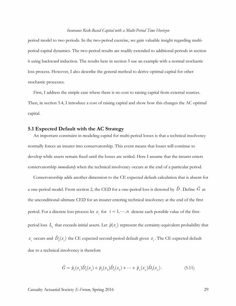
5.1 Expected Default with the AC Strategy An important constraint in modeling capital for multi-period losses is that a technical insolvency
normally forces an insurer into conservatorship. This event means that losses will continue to
develop while assets remain fixed until the losses are settled. Here I assume that the insurer enters
conservatorship immediately when the technical insolvency occurs at the end of a particular period.
Conservatorship adds another dimension to the CE expected default calculation that is absent for
a one-period model. From section 2, the CED for a one-period loss is denoted by . Define as
the unconditional ultimate CED for an insurer entering technical insolvency at the end of the first
period. For a discrete loss process let for denote each possible value of the first-
period loss that exceeds initial assets. Let represent the certainty-equivalent probability that
occurs and the CE expected second-period default given . The CE expected default
due to a technical insolvency is therefore
. (5.11)

Insurance Risk-Based Capital with a Multi-Period Time Horizon
Casualty Actuarial Society E-Forum, Spring 2016 30
To illustrate this, I approximate a normal stochastic loss process using a discrete probability
distribution for the independent loss increments. This numerical example is shown in Appendix A.
The value of is 0.9029, which exceeds the first-period value of 0.3144.
Observe that depends on the variance of loss development beyond the first period (i.e., the
ultimate variance), while only depends on volatility during the first period. For a positive second-
period variance, the mathematical properties of the default calculation ensure that is greater than
that of the original first-period default: cannot be negative; it equals zero if the loss develops
favorably. This asymmetry increases the expected ultimate default amount beyond its initial first-
period value regardless of the first-period loss amount.
5.2 Optimal Two-period AC Capital A particular value of initial capital C will establish the assets A available to pay the loss at the end
of the first period (equation 4.31). This asset amount will thus uniquely determine the CE expected
default for the first period, as discussed in section 5.1. The amount A will also uniquely
determine the CED for the second period since the capital strategy is predetermined. The total CE
expected default for the insurer is the sum of the CED values for the first and second periods.
For a continuous distribution of losses, with x denoting the first period loss value, the equivalent
of equation 5.11 is
. (5.21)
If the insurer remains solvent at the end of the first period, there is one period remaining: it can
become insolvent at the end of the second period. However, from section 2, for each loss value
there is an optimal amount of capital and a corresponding optimal CED amount, represented by
Insurance Risk-Based Capital with a Multi-Period Time Horizon
Casualty Actuarial Society E-Forum, Spring 2016 31
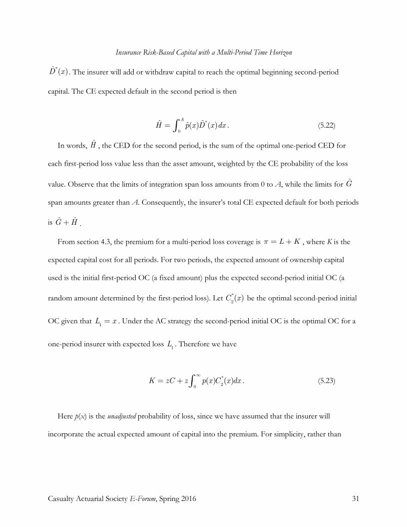
. The insurer will add or withdraw capital to reach the optimal beginning second-period
capital. The CE expected default in the second period is then
. (5.22)
In words, , the CED for the second period, is the sum of the optimal one-period CED for
each first-period loss value less than the asset amount, weighted by the CE probability of the loss
value. Observe that the limits of integration span loss amounts from 0 to A, while the limits for
span amounts greater than A. Consequently, the insurer’s total CE expected default for both periods
is .
From section 4.3, the premium for a multi-period loss coverage is , where K is the
expected capital cost for all periods. For two periods, the expected amount of ownership capital
used is the initial first-period OC (a fixed amount) plus the expected second-period initial OC (a
random amount determined by the first-period loss). Let be the optimal second-period initial
OC given that . Under the AC strategy the second-period initial OC is the optimal OC for a
one-period insurer with expected loss . Therefore we have
. (5.23)
Here p(x) is the unadjusted probability of loss, since we have assumed that the insurer will
incorporate the actual expected amount of capital into the premium. For simplicity, rather than

Insurance Risk-Based Capital with a Multi-Period Time Horizon
Casualty Actuarial Society E-Forum, Spring 2016 32
using the asset value A, I have used an infinite upper limit.20
The consumer value of the insurance transaction is . The optimal initial
available asset value is found by maximizing V, or alternatively, minimizing the solvency cost
. (5.24)
Because is not analytically tractable for important probability distributions such as the normal,
we need to use numerical approximation methods to find the optimal assets in these cases. Once the
optimal assets are found, we use equation 4.31 to determine the optimal capital. Section 5.3 outlines
an approach for the normal and lognormal stochastic processes.
For the FR strategy, the insurer is recapitalized at the end of the first period to the optimal
second-period amount. So, viewed from the beginning of the first period, the solvency cost for the
second period is the optimal amount for that period as if we had just begun that period. Therefore,
the initial capital for the first period is independent of the second-period loss distribution, and
depends only on the potential loss values for the first period.
Section 5.1 showed that, for a given initial asset level, the CE expected default for the AC strategy
is higher than that for the FR strategy. This implies that the optimal initial total capital for the AC
strategy is higher than for the FR strategy, which is the theoretically most efficient strategy. This result
is reflected in the section 5.3 numerical examples with the normal stochastic loss process.
To prove this result, assume that we use an AC strategy, but the initial total capital is the optimal
total capital for an FR strategy. The AC certainty-equivalent default is greater than the optimal
CED under FR. Also, the derivative is a weighted average of the values for losses
20 The error in this approximation will be small if the default probability is small. In the section 5.3 example, the difference in optimal capital is 333.34 – 333.15 = 0.19, an error of 0.06%.
Insurance Risk-Based Capital with a Multi-Period Time Horizon
Casualty Actuarial Society E-Forum, Spring 2016 33
greater than A. Each of the component values in the weighted average is higher than z, so adding
capital at the margin will reduce more than it will increase the capital cost. Consequently, the
optimal AC total capital will be greater than the optimal FR total capital21 for two periods and the
optimal AC solvency cost will be greater as well.
5.3 Optimal Two-period Capital for Normal Stochastic Processes In this section I use the normal stochastic process from section 4.2 to calculate numerical results.
Here the period-ending loss distribution is normal. This distribution is continuous, and serves to
illustrate dynamic loss development. The policyholder risk aversion is based on exponential utility;
thus optimal capital can be determined from the resulting CE values, as shown in Appendix B. The
numerical example developed here is expanded in subsequent sections to demonstrate results for
variations of the basic model. These results are intended to elucidate the general method for
determining optimal capital; a practical application will likely involve more complex modeling.
Although the lognormal loss process is perhaps better suited to modeling insurance loss
development,22 I have chosen to use the normal model, which is simpler to explain and which
provides tractable results for a joint loss and asset distribution (see section 9). Under the lognormal
process, the conditional one-period optimal capital and CED are proportional to the expected loss,
while under the normal distribution, these values are independent of the expected loss. The results
for a lognormal loss process are similar, 23 however.
21 Since the premium contains the expected capital cost for both periods, the optimal first-period FR ownership capital equals the optimal OC for a one-period model, less the expected capital cost for the second period. Essentially, in this case, compared to the one-period model, the policyholder has prepaid the second-period capital cost, so the optimal initial ownership capital is less than in the one-period model by the amount of the prepayment. 22 The lognormal distribution has been used by several authors (see Wacek [2007] and Han and Goa [2008]) to analyze the variability of loss reserves. 23 For the same periodic loss volatility, the optimal capital for the lognormal process is slightly higher than that for the normal counterpart.

Insurance Risk-Based Capital with a Multi-Period Time Horizon
Casualty Actuarial Society E-Forum, Spring 2016 34
With a normal loss process, the optimal capital and CED for one period are constants
independent of the expected loss (but are a function of the standard deviation). This property
facilitates the calculation of optimal capital for two or more periods. Appendix B develops a
numerical example to illustrate optimal capital under the normal stochastic loss process with
exponential utility, which is labeled as the normal-exponential model. I extend the example to
illustrate results in subsequent sections of the paper.
The example uses a two-period normal stochastic loss process with a mean of 1000 and variance
of the loss increment equal to 1002 for each period. The CE value of the expected loss after one
period is 1050 and the risk value (the CE of the loss minus its expected value) at each development
stage is strictly proportional to the cumulative variance as in section 4.22. Thus, the CE value of the
ultimate loss at the end of the second period is 1100.
The frictional capital cost is z = 2%. The optimal one-period total capital is 291.62 and the
optimal two-period initial total capital is 333.34.
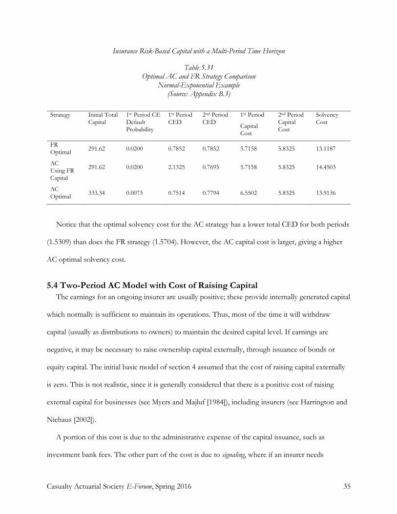
Table 5.31 summarizes the optimal AC results. Here I compare the optimal two-period AC
strategy with that of the optimal FR strategy. The table also shows results for the AC strategy using
the optimal FR initial total capital as the initial capital for the AC strategy.
Insurance Risk-Based Capital with a Multi-Period Time Horizon
Casualty Actuarial Society E-Forum, Spring 2016 35
Table 5.31 Optimal AC and FR Strategy Comparison
Normal-Exponential Example (Source: Appendix B.3)
Strategy Initial Total
Capital 1st Period CE Default Probability
1st Period CED
2nd Period CED
1st Period
Capital Cost
2nd Period Capital Cost
Solvency Cost
FR Optimal 291.62 0.0200 0.7852 0.7852 5.7158 5.8325 13.1187
AC Using FR Capital
291.62 0.0200 2.1325 0.7695 5.7158 5.8325 14.4503
AC Optimal 333.34 0.0073 0.7514 0.7794 6.5502 5.8325 13.9136
Notice that the optimal solvency cost for the AC strategy has a lower total CED for both periods
(1.5309) than does the FR strategy (1.5704). However, the AC capital cost is larger, giving a higher
AC optimal solvency cost.
5.4 Two-Period AC Model with Cost of Raising Capital The earnings for an ongoing insurer are usually positive; these provide internally generated capital
which normally is sufficient to maintain its operations. Thus, most of the time it will withdraw
capital (usually as distributions to owners) to maintain the desired capital level. If earnings are
negative, it may be necessary to raise ownership capital externally, through issuance of bonds or
equity capital. The initial basic model of section 4 assumed that the cost of raising capital externally
is zero. This is not realistic, since it is generally considered that there is a positive cost of raising
external capital for businesses (see Myers and Majluf [1984]), including insurers (see Harrington and
Niehaus [2002]).
A portion of this cost is due to the administrative expense of the capital issuance, such as
investment bank fees. The other part of the cost is due to signaling, where if an insurer needs
Insurance Risk-Based Capital with a Multi-Period Time Horizon
Casualty Actuarial Society E-Forum, Spring 2016 36
additional capital due to low earnings, investors may believe that the management is poor. Thus, the
capital suppliers will require a high return on the capital provided and the value of the company to
existing shareholders will be diluted. This effect is especially prominent when most other insurers do
not require additional capital.24
5.41 Linear Model for Cost of Raising Capital To model the cost of raising capital (abbreviated by CRC), assume that the cost is a rate w times
the amount of capital raised.25 We continue to assume that no capital is raised if the insurer is
technically insolvent. Also assume that the insurer is already in business, so that its first-period
capital is not raised externally.26
For a two-period model, at the end of the first period, there is one period remaining. If it is not
necessary to raise capital, the optimal capital for the beginning of the second period is determined by
equation 2.23. However, if capital is raised at that point, there is an additional capital cost w to the
insurer beyond z, the cost of holding capital.
Let represent the initial second-period ownership capital after having raised capital and
the ending first period OC. Thus, the amount of capital raised is . We need to distinguish
between the optimal amount of capital given that it is raised externally and the amount if it is
generated internally. Hence the distinct notation for the capital amount given that it is raised
externally. The total capital cost in the second period is then .
24 In the event of an industry-wide catastrophe or pricing cycle downturn, the signaling effect may not be significant. In fact, the prospect of near-term increased insurance prices can spur investment in the property-casualty industry. 25 An alternative formulation is to assume that the cost of raising capital increases as the insurer nears insolvency, but this will be more difficult to model. 26 The one-period model in EBRM implicitly assumed that there was no cost of raising capital. A solvent ongoing insurer with one-period losses will need to raise capital (to the optimal level for the next group of policyholders) if the ending loss amount is large enough. This effect will change the optimal initial capital slightly.

Insurance Risk-Based Capital with a Multi-Period Time Horizon
Casualty Actuarial Society E-Forum, Spring 2016 37
Because the marginal amount of capital raised carries a cost of z + w, following the section 2.2
analysis, the optimal second period capital, given that it is externally raised, is determined by
, (5.411)
where A2 is the second-period available assets. Since we assume that w is positive, the optimal
second-period capital with a CRC is less than that if there were no CRC: since new capital raised is
expensive with a CRC, the insurer will use less of it; the policyholder is satisfied, having achieved the
optimal balance of price and security. Denote the optimal second-period OC, given that capital is
raised externally at the end of the first period, by .
5.42 Optimal Two-Period Capital with CRC With a positive cost of raising capital, we can modify the AC strategy to produce an optimal
initial capital amount. To distinguish an AC capital strategy with a positive cost of raising capital
from one with a zero cost, I abbreviate the CRC version to ACR.
Under the dynamic ACR strategy, the CRC is incurred if the first-period loss estimate is such
that the ending first-period OC is between zero and . Thus, the capital flows depend on four
distinct regions based on the first-period ending OC amount CE . To illustrate this, I expand Table
4.51 by splitting region 2 into two sub-regions. Table 5.421 shows the capital flows by region:
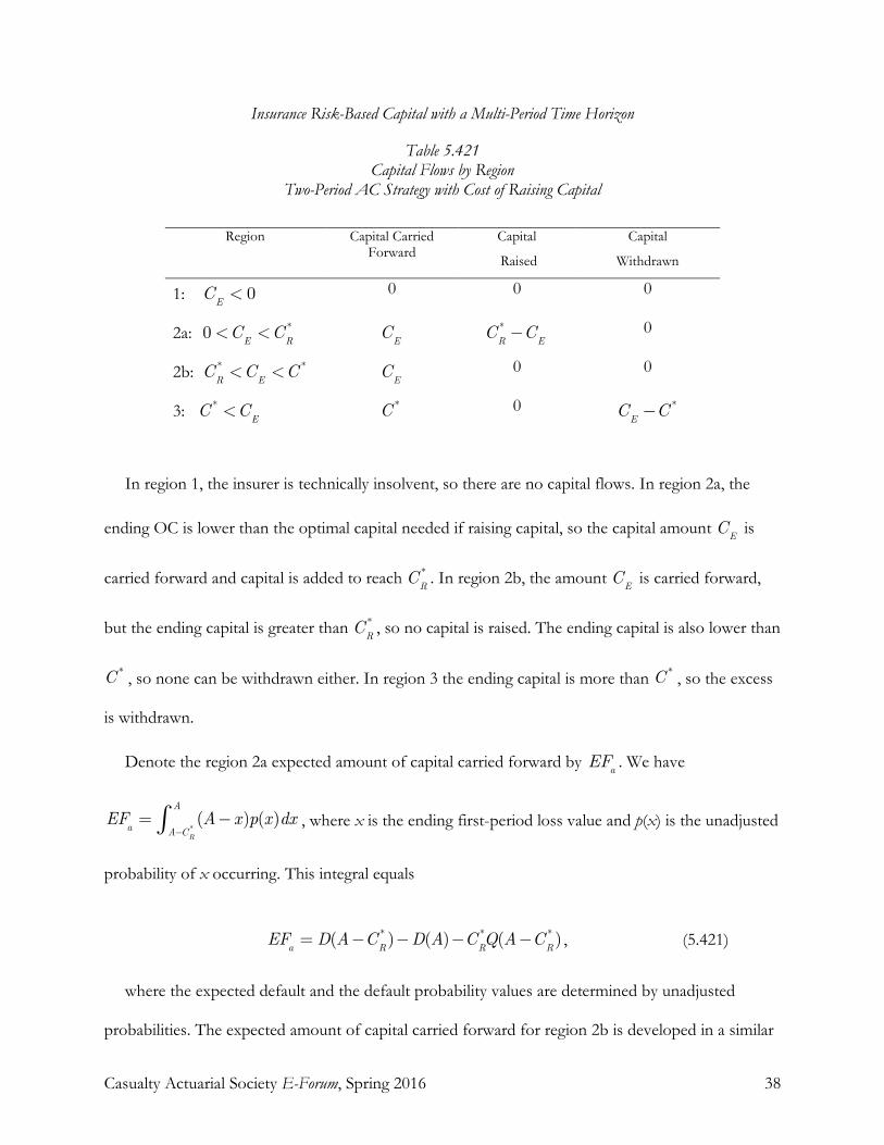
Insurance Risk-Based Capital with a Multi-Period Time Horizon
Casualty Actuarial Society E-Forum, Spring 2016 38
Table 5.421 Capital Flows by Region
Two-Period AC Strategy with Cost of Raising Capital
Region Capital Carried Forward
Capital
Raised
Capital
Withdrawn
1: 0 0 0
2a: 0
2b: 0 0
3: 0
In region 1, the insurer is technically insolvent, so there are no capital flows. In region 2a, the
ending OC is lower than the optimal capital needed if raising capital, so the capital amount is
carried forward and capital is added to reach . In region 2b, the amount is carried forward,
but the ending capital is greater than , so no capital is raised. The ending capital is also lower than
, so none can be withdrawn either. In region 3 the ending capital is more than , so the excess
is withdrawn.
Denote the region 2a expected amount of capital carried forward by . We have
, where x is the ending first-period loss value and p(x) is the unadjusted
probability of x occurring. This integral equals
, (5.421)
where the expected default and the default probability values are determined by unadjusted
probabilities. The expected amount of capital carried forward for region 2b is developed in a similar
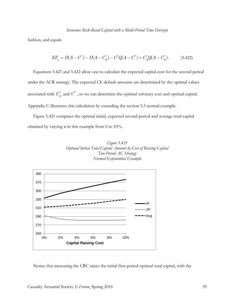
Insurance Risk-Based Capital with a Multi-Period Time Horizon
Casualty Actuarial Society E-Forum, Spring 2016 39
fashion, and equals
. (5.422)
Equations 5.421 and 5.422 allow one to calculate the expected capital cost for the second period
under the ACR strategy. The expected CE default amounts are determined by the optimal values
associated with and , so we can determine the optimal solvency cost and optimal capital.
Appendix C illustrates this calculation by extending the section 5.3 normal example.
Figure 5.421 compares the optimal initial, expected second-period and average total capital
obtained by varying w in this example from 0 to 10%.
Figure 5.421 Optimal Initial Total Capital Amount by Cost of Raising Capital
Two-Period AC Strategy Normal-Exponential Example
Notice that increasing the CRC raises the initial first-period optimal total capital, with the
250
270
290
310
330
350
370
390
0% 2% 4% 6% 8% 10%Capital Raising Cost
IP
2P
Avg
Insurance Risk-Based Capital with a Multi-Period Time Horizon
Casualty Actuarial Society E-Forum, Spring 2016 40
expected second-period optimal capital being lower than that for the optimal one-period capital. The
second-period capital is diminished because the second-period capital cost goes up due to the CRC
and the insurer (on behalf of the policyholder) will use less of it. The initial capital increases because
the insurer will avoid some of the high second-period cost by having a higher initial capital and
carrying more of it into the second period. Also notice that increasing the CRC also raises the
average amount of capital over both periods.
The capital raising cost will vary by insurer, and is likely to be lower for established insurers with
better access to the capital markets. Thus, the CRC is another variable to consider when assessing
risk-based capital.27
5.5 Insurers with Limited Ability to Raise Capital Besides depending on the cost of raising capital, the optimal capital amount also depends on the
ability of insurers to raise capital. It is well-known that the organizational form of insurers dictates
how they may raise capital (see Harrington and Niehaus [2002] and Cummins and Danzon [1997]).
In particular, depending on the details of their structure, mutual insurers may have difficulty raising
capital externally.28 In the case where an insurer cannot raise external capital, the best capital strategy
is capital withdrawal (CW). Note however, that this strategy will represent an upper limit to optimal
capital for a mutual insurer, since the insurer can raise additional capital internally by charging its
policyholders a higher premium.29
27 With a CRC, even under a FR strategy the optimal initial capital will be larger than without the CRC, since capital must be stockpiled early to avoid the cost of subsequently raising it. Thus, for the FR strategy with a CRC the initial capital depends on the volatility of future losses, not just the behavior of current period losses. 28 Some mutual insurers have issued surplus notes, which are similar to equity in terms of capital structure, but are a type of risky bond to investors. According to A.M. Best [2003], the major issuers of surplus notes were usually large insurers with more access to capital markets, while small or mid-size insurers could only issue surplus notes in limited amounts with short maturity. 29 However, this method is limited since the policyholders will tend to migrate to other insurers if the premium is too high.
Insurance Risk-Based Capital with a Multi-Period Time Horizon
Casualty Actuarial Society E-Forum, Spring 2016 41
Under CW, all capital flows (except for the initial capitalization) are withdrawals; capital increases
arise from positive earnings. Using the section 5.4 example, the optimal initial CW total capital
amount is 433.61, with an expected second-period optimal capital of 291.62 and average over the
two periods of 362.62. The solvency cost of this optimum position is 16.29. For comparison, the
solvency cost of the section 5.42 AC strategy with a 4% CRC is 14.76.
Harrington and Niehaus show that mutual insurers carry more capital than stock insurers having
the same risk. This result supports the analysis presented here.
Although the solvency cost (and hence the consumer value) for the mutual insurer is inferior to
that of the section 5.4 insurer, the policyholder is not necessarily worse off. A mutual policyholder is also
an owner of the insurer and receives dividends if the mutual is profitable. These distributions are not
taxable at the personal income level. However, a similar policyholder of a stock insurer with an
equivalent stake in that insurer would be subject to income taxes on the capital distributions. This
tax-free benefit increases the consumer value of the mutual insurance purchase. To illustrate,
suppose that the personal income tax rate on the capital distributions is 20% and the expected return
on capital is 8%. The average ownership capital for the section 5.4 stock insurer (with
w = 4%) is 317.30. Thus, the expected return to the policy/equity holder is 25.38. The tax on this
amount is 5.08 = 0.20(25.38). The stock policyholder’s consumer value after the personal income tax
is the risk value minus the solvency cost minus the income tax: 80.16 = 100.00 – 14.76 – 5.08. The
mutual policyholder’s consumer value, with no personal income tax, is in fact higher: 83.71 = 100.00
– 16.29.
To the extent that regulatory capital requirements are related to the optimal capital that insurers
might carry, then the analysis here suggests that risk-based capital should be higher for mutual insurers
than for stock insurers having the same default risk.
Insurance Risk-Based Capital with a Multi-Period Time Horizon
Casualty Actuarial Society E-Forum, Spring 2016 42
6. OPTIMAL CAPITAL FOR MORE THAN TWO PERIODS
This section determines optimal capital for multiple periods by extending the two-period model
for the capital strategies using the backward induction method. Here I outline the method generally
and apply it to the AC and ACR strategies.
6.1 General Backward Induction Method The backward induction method determines a sequence of optimal actions or results by starting
from the end of a problem with discrete stages and working backwards in time, to the beginning of
the problem. It uses the output of each prior stage to determine an optimal action based on the
information available for the particular stage. This course proceeds backwards until one has
determined the best action for every possible situation at every point in time. Backward induction is
used extensively in dynamic programming and game theory.30
To apply backward induction for a capital strategy where there is no CRC, define an index i for
each stage, where i is the number of periods remaining until the ultimate loss is determined. At each
stage i, we use three optimal quantities that have been determined from the prior stage, and may
depend on the loss value x from stage i: the optimal ownership capital , the optimal CED
and the optimal capital cost .
For stage i, we start with the optimal asset amount from the prior stage i – 1 and calculate the
solvency cost. We vary the asset amount until the optimal solvency cost is attained, and record the
values of the above three optimal quantities. The process is repeated until the Nth stage is complete.
The result is the optimal initial capital, CED and capital cost for an N-period model. The
intermediate stage results will give the optimal quantities for all models of lesser duration that have
30 For example, see Von Neumann and Morgenstern [1944].
Insurance Risk-Based Capital with a Multi-Period Time Horizon
Casualty Actuarial Society E-Forum, Spring 2016 43
the same sequence of loss increment variances per period.31 Accordingly, for a model with constant
volatility per period, we will get the optimal results for all models with N or fewer periods.
6.2 Backward Induction Method with AC Strategy Under the AC capital strategy for stage i, the solvency cost has four components:
(1) the CED for technical insolvency in the stage, (2) the expected CED for future insolvency, (3)
the capital cost for the stage and (4) the expected future capital costs. The first two components
represent the total CED for all periods through stage i, denoted by , and the last two represent
, the total capital cost for all periods. Therefore we can represent the solvency cost as
, where
(6.21)
and
. (6.22)
We minimize the value of to get the optimal available asset value for this stage.32 From
equation 4.31, we get the optimal OC:
. (6.23)
The optimal total capital is . We also have optimal values of the components ,
31 For example, suppose a three-period model has a standard deviation (SD) of 50 for the first period loss increment, 60 for the second period and 80 for the third period. This process will provide optimal results for the three-period case and will also give the optimal results for a one-period model with an 80 SD, and a two-period model with a 60 SD for the first period and 80 for the second period. 32 Appendix C discusses the optimization technique, which uses two asset values whose difference is small.
Insurance Risk-Based Capital with a Multi-Period Time Horizon
Casualty Actuarial Society E-Forum, Spring 2016 44
and , which we label and . So now we have the three inputs needed to determine the
optimal capital for the stage i + 1, and successive stages, until the optimal initial capital for the Nth
period is found.
To illustrate this process, consider the basic section 5 example from Appendix B. We have =
0.7852 (from Appendix B.1) and = 5.8325 (from Appendix B.3). Applying equations 6.21 and
6.22, and iterating gives the following optimal values for a time horizon ranging from 1 through 4
periods.
Table 6.21 Optimal Values by Number of Periods
Normal-Exponential Example; AC Strategy
No. of
Periods
Initial Total
Capital CED
Capital
Cost
Ownership
Capital
1 291.62 0.7852 5.8325 291.62
2 333.34 1.5309 12.3827 327.51
3 354.95 2.2367 19.2317 342.45
4 365.70 2.9212 26.1537 346.10
Extending the example to 20 periods, Figure 6.21 compares optimal initial total capital (TC) and
ownership capital (OC) amounts by period length.
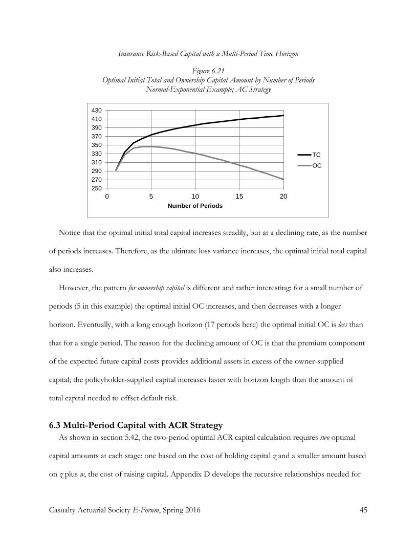
Insurance Risk-Based Capital with a Multi-Period Time Horizon
Casualty Actuarial Society E-Forum, Spring 2016 45
Figure 6.21 Optimal Initial Total and Ownership Capital Amount by Number of Periods
Normal-Exponential Example; AC Strategy
Notice that the optimal initial total capital increases steadily, but at a declining rate, as the number
of periods increases. Therefore, as the ultimate loss variance increases, the optimal initial total capital
also increases.
However, the pattern for ownership capital is different and rather interesting: for a small number of
periods (5 in this example) the optimal initial OC increases, and then decreases with a longer
horizon. Eventually, with a long enough horizon (17 periods here) the optimal initial OC is less than
that for a single period. The reason for the declining amount of OC is that the premium component
of the expected future capital costs provides additional assets in excess of the owner-supplied
capital; the policyholder-supplied capital increases faster with horizon length than the amount of
total capital needed to offset default risk.
6.3 Multi-Period Capital with ACR Strategy As shown in section 5.42, the two-period optimal ACR capital calculation requires two optimal
capital amounts at each stage: one based on the cost of holding capital z and a smaller amount based
on z plus w, the cost of raising capital. Appendix D develops the recursive relationships needed for
250270290310330350370390410430
0 5 10 15 20Number of Periods
TC
OC
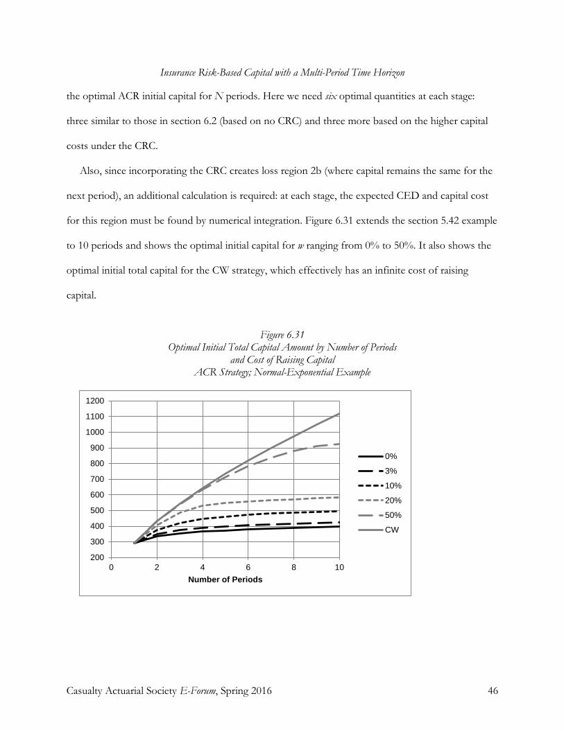
Insurance Risk-Based Capital with a Multi-Period Time Horizon
Casualty Actuarial Society E-Forum, Spring 2016 46
the optimal ACR initial capital for N periods. Here we need six optimal quantities at each stage:
three similar to those in section 6.2 (based on no CRC) and three more based on the higher capital
costs under the CRC.
Also, since incorporating the CRC creates loss region 2b (where capital remains the same for the
next period), an additional calculation is required: at each stage, the expected CED and capital cost
for this region must be found by numerical integration. Figure 6.31 extends the section 5.42 example
to 10 periods and shows the optimal initial capital for w ranging from 0% to 50%. It also shows the
optimal initial total capital for the CW strategy, which effectively has an infinite cost of raising
capital.
Figure 6.31 Optimal Initial Total Capital Amount by Number of Periods
and Cost of Raising Capital ACR Strategy; Normal-Exponential Example
200
300
400
500
600
700
800
900
1000
1100
1200
0 2 4 6 8 10Number of Periods
0%
3%
10%
20%
50%
CW

Insurance Risk-Based Capital with a Multi-Period Time Horizon
Casualty Actuarial Society E-Forum, Spring 2016 47
7. CAPITALIZATION INTERVAL
The preceding analysis has used an arbitrary period length, with capital flows occurring at the
beginning of each period. Since the period length governs the duration between capital flows, and to
distinguish it from other insurance periods such as policy term, I specifically refer to the period
length as the capitalization interval (abbreviated as CI).
The actual length of the CI will affect the optimal capital, since, for a given loss duration, a
shorter capitalization interval will allow more opportunities to add or withdraw capital as the loss
amount evolves. To analyze this effect, recall that the policy term is defined to be equal to the period
length. Thus, the losses occur at the beginning of the policy term,33 and capital flows also occur at
the beginning and end of the policy term. Section 7.3 discusses the case where the period length is
shorter than the policy term.
The frequency of potential capital additions and withdrawals will have a significant impact on the
optimal capital and solvency cost, regardless of the capital strategy used.
7.1 Capitalization Interval with the FR Strategy To illustrate the effect of the CI, again assume the basic one-period normal example from section
5 with a standard deviation of 100. The optimal total capital is 291.62 with a solvency cost of 6.62.
The period length and loss duration are both one year: thus, capital is supplied at the beginning of the
year and the amount of loss is known at the end of the year. Also assume that the stochastic process
is continuous over time: for every smaller period the loss variance is proportional to the period
length. Now suppose that we subdivide the one-year period into half-year periods, with capital flows
allowed at the beginning of each. Each smaller period will now have a loss standard deviation of
33 A more realistic assumption is that the loss may occur randomly throughout the policy term, with the average loss happening at the middle of the term. Here, I am merely attempting to show the effect of changing the capitalization interval length. A practical application would use the actual expected timing of the incurred losses.
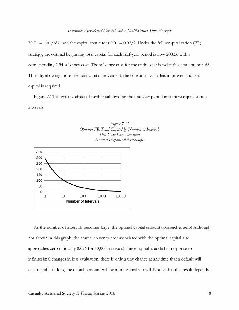
Insurance Risk-Based Capital with a Multi-Period Time Horizon
Casualty Actuarial Society E-Forum, Spring 2016 48
70.71 = and the capital cost rate is 0.01 = 0.02/2. Under the full recapitalization (FR)
strategy, the optimal beginning total capital for each half-year period is now 208.56 with a
corresponding 2.34 solvency cost. The solvency cost for the entire year is twice this amount, or 4.68.
Thus, by allowing more frequent capital movement, the consumer value has improved and less
capital is required.
Figure 7.11 shows the effect of further subdividing the one-year period into more capitalization
intervals:
Figure 7.11 Optimal FR Total Capital by Number of Intervals
One-Year Loss Duration Normal-Exponential Example
As the number of intervals becomes large, the optimal capital amount approaches zero! Although
not shown in this graph, the annual solvency cost associated with the optimal capital also
approaches zero (it is only 0.096 for 10,000 intervals). Since capital is added in response to
infinitesimal changes in loss evaluation, there is only a tiny chance at any time that a default will
occur, and if it does, the default amount will be infinitesimally small. Notice that this result depends
050
100150200250300350
1 10 100 1000 10000Number of Intervals

Insurance Risk-Based Capital with a Multi-Period Time Horizon
Casualty Actuarial Society E-Forum, Spring 2016 49
on the assumption of a continuous distribution for the loss increment: if the loss valuation can change
in somewhat large increments, then the capital additions cannot “catch up.” Consequently, in a
theoretical world with a continuous stochastic loss process and the ability to add capital with no
cost, there is no need for an insurer to carry capital. However, the loss process might not be
continuous, and, as discussed next in section 7.2, important real-world imperfections, frictions and
costs do not permit an infinitesimally small CI, so capital is indeed required.
7.2 Capital Strategies and Time Intervals For other capital strategies, the optimal capital also declines as the CI becomes smaller. Figure
7.21 compares results of the FR, AC, CW and ACR (with 5% cost of raising capital) strategies,
according to interval length. Here, I show the average amount of total capital over the year. Note that
the initial capital for the first period will also decline with the number of intervals for the FR, AC
and ACR with low capital-raising cost strategies. However, for the CW and high capital-raising cost
ACR strategies, the first-period capital amount increases with the number of intervals. Nevertheless,
since these strategies stockpile capital in the early periods and tend to withdraw more of it later than
for the other strategies, the average amount of capital declines with the number of intervals.
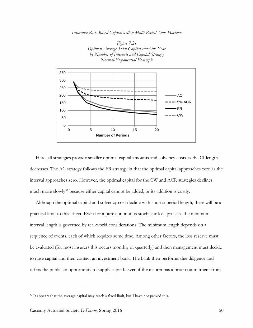
Insurance Risk-Based Capital with a Multi-Period Time Horizon
Casualty Actuarial Society E-Forum, Spring 2016 50
Figure 7.21 Optimal Average Total Capital For One Year by Number of Intervals and Capital Strategy
Normal-Exponential Example
Here, all strategies provide smaller optimal capital amounts and solvency costs as the CI length
decreases. The AC strategy follows the FR strategy in that the optimal capital approaches zero as the
interval approaches zero. However, the optimal capital for the CW and ACR strategies declines
much more slowly34 because either capital cannot be added, or its addition is costly.
Although the optimal capital and solvency cost decline with shorter period length, there will be a
practical limit to this effect. Even for a pure continuous stochastic loss process, the minimum
interval length is governed by real-world considerations. The minimum length depends on a
sequence of events, each of which requires some time. Among other factors, the loss reserve must
be evaluated (for most insurers this occurs monthly or quarterly) and then management must decide
to raise capital and then contact an investment bank. The bank then performs due diligence and
offers the public an opportunity to supply capital. Even if the insurer has a prior commitment from
34 It appears that the average capital may reach a fixed limit, but I have not proved this.
0
50
100
150
200
250
300
350
0 5 10 15 20Number of Periods
AC
5% ACR
FR
CW

Insurance Risk-Based Capital with a Multi-Period Time Horizon
Casualty Actuarial Society E-Forum, Spring 2016 51
an investment bank, this process may take several months.
Nevertheless, it is clear that policies with short capitalization intervals will require less capital than
longer ones, and will be more efficient (with lower solvency costs) as well.35 Because some insurers
may be better-equipped to generate capital flows quickly, the minimum interval length will vary by
insurer. Consequently, this factor should be considered in assessing specific insurer capital levels.
7.3 Effect of Policy Term and Capitalization Interval The preceding analysis has assumed that the capitalization interval equals the policy term.
Generally, the policy term for property-casualty insurance is one year,36 but the capitalization interval
will most likely be shorter than one year. Assume that the premium is paid at the beginning of the
period. When the capitalization interval is shorter than the policy term, insolvency may occur early in
the policy term. This event will effectively terminate coverage for losses that may occur in the
remainder of the policy term, and will produce an additional solvency cost, since the full premium is
paid up front.
Here, more capital is needed if the policy term exceeds the CI, regardless of the number of
intervals. Thus, besides the CI, which greatly affects the optimal capital, the length of the policy term is
another variable that will influence the capital amount. This effect will be present with both short-
duration and long-duration37 losses, since the cost of foregone coverage must be considered.
35 Because the ability to quickly raise capital decreases solvency costs, the capitalization interval length will also affect short-duration losses in a manner similar to that of long-duration losses: optimal capital is less if the CI length is shortened. 36 Some automobile policies have a six-month term and, less commonly, some commercial risks have multi-year coverage. 37 Modeling this effect is more complicated than for property, since one must assume a relationship between the losses of each interval. For liability coverage, these will be correlated. A convenient approach is to assume that all losses move together.

Insurance Risk-Based Capital with a Multi-Period Time Horizon
Casualty Actuarial Society E-Forum, Spring 2016 52
8. MULTI-PERIOD MODEL EXTENSIONS
This section extends the basic loss model to incorporate features that may be necessary for a
practical application. Also, I briefly discuss how the results might apply to life insurance.
8.1 Stochastic Time Horizon In a more realistic model of the development process for long-duration losses, the ultimate
duration of losses is not known. Here I relax the basic model assumption that the loss develops
randomly for N periods and is settled at the end of the Nth period. Instead, assume that, although
the value evolves according to the section 4.2 liability stochastic process, the process may terminate
randomly at the end of each period, at which point the loss is settled. In this model, there are N
possible periods, extending to the longest possible claim duration. Call this model the stochastic-
horizon (abbreviated as SH) loss model.
Let represent the probability of settlement at the end of period i. Then .
From section 4.21, with a constant per-period loss volatility the variance of the ultimate loss will be
, since the variance of each period’s loss increment is independent of
the prior value. This is a simple weighted average of the loss variances of the component N possible
models.
Meanwhile, assume that the certainty-equivalent expected value of the SH loss is proportional to
the variance (as discussed in section 4.42). Consequently, the CE expected value of the SH loss must
equal the weighted average of the CE expected loss values of its N component loss models, where
the weights are the termination probabilities .
Under the SH model, the optimal capital will be a weighted average of the optimal capital values
for the component fixed-horizon models. Given the above analysis, to approximate the optimal SH
Insurance Risk-Based Capital with a Multi-Period Time Horizon
Casualty Actuarial Society E-Forum, Spring 2016 53
capital, it is reasonable to use the exact termination probabilities (rather than a CE adjusted set of
probabilities) to weight the optimal capital amounts.
To illustrate the SH model, we extend the basic normal-exponential example. Assume three
periods with termination probabilities = 0.5, = 0.3 and = 0.2. The average loss duration is
1.7 periods and the respective expected amounts of loss paid at the end of each period are 500, 300
and 200. From section 6.2, the optimal initial total capital amounts for the three component
horizons are = 291.62, = 333.34 and = 354.95. Thus, the optimal initial capital for the
basic SH model is 316.80 = 0.5(291.62) + 0.3(333.34) + 0.2(354.95).
Notice that, if the expected loss is independent of the loss duration (as in the basic model) the set
of termination probabilities will represent the expected loss payment pattern.
8.2 Interest Rates and Present Values Because multi-period losses, especially for liability insurance, can be paid several years from when
the loss occurs, it is necessary to use the present value of the solvency cost components in determining
optimal capital. Since the present value of a certainty-equivalent amount must also be a CE value,
the present value is found using a risk-free interest rate, denoted by a rate r per period. A similar logic
applies to the capital cost component. Note that this assumption of a single rate implies a flat yield
curve; a practical application might require a separate riskless rate for each component duration.
For a one-period model, the present value of the solvency cost is
. (8.21)
The initial assets equal the capital plus the premium. The premium is ,
Insurance Risk-Based Capital with a Multi-Period Time Horizon
Casualty Actuarial Society E-Forum, Spring 2016 54
which equals the present value of the expected loss and capital cost components. At the end of the
period, before the loss and capital costs are paid, the initial assets grow to . The
capital cost zC is expended prior to the loss payment, so the assets available to pay the loss are
. Thus . Also, from section 2.2 we have
. The optimal solvency cost is found from , giving
. (8.22)
The amount z/(1 + r) is the calibration level of the risk measure . With r = 0, we have
, the result used in the earlier sections of this paper. With zero interest, we find the
optimal assets satisfying the calibration level and subtract the expected loss amount to get the
optimal capital. With a positive r, however, equation 8.22 gives the ending available assets; subtracting
the expected loss gives the ending optimal capital, which must be reduced by a factor of 1 + r to
produce the optimal initial capital. Consequently, the optimal initial capital is the present value of the
amount of capital required with a zero interest rate, where the calibration level equals the present
value of the capital cost rate.
Besides affecting the present value of the optimal capital, the interest rate level will affect the
frictional cost of capital (through double-taxation), as discussed in EBRM. I assume that the
expected default has a negligible impact on the premium. If the insurer’s income tax rate is t, the
frictional cost of capital component due to double taxation for one period equals times
the capital amount. It is useful to separate the frictional cost of capital into two components: the
double-taxation cost, which depends on r and the other costs (such as financial distress and
Insurance Risk-Based Capital with a Multi-Period Time Horizon
Casualty Actuarial Society E-Forum, Spring 2016 55
regulatory restriction costs) that do not depend on r. We then have
. (8.23)
If r = 0, then and the calibration level is . If r > 0, the calibration level is greater than
for . This inequality will hold for plausible values of t and .38 Therefore, the
optimal capital amount from equation 8.22 will be less than the present value of the zero-interest
optimal capital, since the calibration level is lower (making capital more costly).
To illustrate the effect of the interest rate on optimal capital, I modify the basic section 5.3
example for one period. Assume that = 0.5% and t = 30%. With r = 0, we have z = 0.5% from
equation 8.23, giving a 0.5% calibration level and optimal capital of 347.59. Increasing r to 5%
boosts the calibration level to 2.52% and the optimal capital drops to 267.69. This amount is
significantly less than the present value of zero-interest optimal capital: 331.08 = 347.59/1.05.
The above analysis shows that the interest rate level reduces optimal capital (from that with zero
interest) in two ways. First, there is a present value effect: since the initial capital grows at the rate r,
less capital is needed to offset a potential default occurring in the future. Secondly, the frictional cost
of capital is greater due to double-taxation on the increased investment income from capital: since
the cost of capital is greater, insurers will use less of it.
For a multi-period model, interest rates can readily be incorporated by modifying the section 6
backward induction method. To illustrate, I use the basic AC strategy with no cost of raising capital.
38 The value of is likely to be on the order of magnitude of 1%. Even if the insurer’s effective income tax rate is as
low as 10% (giving =11.1%), the relationship holds.
Insurance Risk-Based Capital with a Multi-Period Time Horizon
Casualty Actuarial Society E-Forum, Spring 2016 56
Let denote the present value of the solvency cost for i periods with interest rate r.
Using the section 6 backward induction indexing, define the present value of the expected capital
cost as , which is the analog of in equation 6.22:
. (8.24)
The solvency cost for stage i is therefore
. (8.25)
The default is realized at the end of i future periods, so its CE expected value is discounted
for i periods. However, the capital costs are discounted for a shorter time span on average, since
they occur over the entire horizon length.
Starting from the one-period optimal CED present value and optimal capital cost
present value , we use equation 8.25 recursively to generate the successive optimal capital
amounts. To demonstrate this calculation, I use the basic AC example from section 6. Figure 8.21
compares the optimal total capital for r ranging from = 0%, to 15%, for horizons of one to ten
periods.
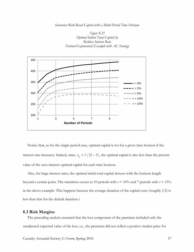
Insurance Risk-Based Capital with a Multi-Period Time Horizon
Casualty Actuarial Society E-Forum, Spring 2016 57
Figure 8.21 Optimal Initial Total Capital by
Riskless Interest Rate Normal-Exponential Example with AC Strategy
Notice that, as for the single-period case, optimal capital is less for a given time horizon if the
interest rate increases. Indeed, since , the optimal capital is also less than the present
value of the zero-interest optimal capital for each time horizon.
Also, for large interest rates, the optimal initial total capital decreases with the horizon length
beyond a certain point. The transition occurs at 10 periods with r = 10% and 7 periods with r = 15%
in the above example. This happens because the average duration of the capital costs (roughly i/2) is
less than that for the default duration i.
8.3 Risk Margins The preceding analysis assumed that the loss component of the premium included only the
unadjusted expected value of the loss, i.e., the premium did not reflect a positive market price for
200
250
300
350
400
450
1 3 5 7 9Number of Periods
r = 0%
r = 2%
r = 5%
r = 10%
r = 15%
Insurance Risk-Based Capital with a Multi-Period Time Horizon
Casualty Actuarial Society E-Forum, Spring 2016 58
bearing the risk. Here I assume that the market value of the insured loss, denoted by , is greater
than the expected loss: i.e., it contains a risk margin, whose value is denoted by M. The expected
market-value loss, including the risk margin, can be determined from a third stochastic process with
an adjusted probability distribution. For a one-period model, we have
, (8.31)
where denotes the adjusted probability underlying the risk margin. Here the relevant risk is
systematic: it cannot be reduced through pooling, and therefore commands a price in financial
markets. The value to the policyholder of the underlying risk, before it is reduced through insurance
pooling, will be larger per unit of expected loss than that of the insurer’s risk (which is larger than
the expected loss). So we have .
For a multi-period stochastic process with equal variance of loss increments for each period, I
assume that the risk margin increases uniformly with the number of periods. In that case, if the
stochastic process is additive, then the risk margin will also be additive. Let m represent the risk
margin as a ratio to the expected loss L for one period. So, for an N-period loss, the risk margin will
equal mLN, and the market value of the expected loss will be L(1 + Nm).
For a multiplicative stochastic process, the market value of L is . Observe that the
present value of the market-value loss is , where r is the risk-free interest rate.
Therefore, the market value of the expected loss can be expressed as the expected value L,
discounted at a risk-adjusted interest rate ,39 where .
39 Butsic [1988] develops the risk-adjusted interest rate for insurance reserving and pricing applications.
Insurance Risk-Based Capital with a Multi-Period Time Horizon
Casualty Actuarial Society E-Forum, Spring 2016 59
The fair premium is . The risk margin then provides additional total capital,
beyond the amount from the expected capital cost K (see section 6.2). The amount M can also be
considered as policyholder-supplied capital; to give the same insolvency protection, the insurer will
need less ownership capital than without the risk margin. As discussed in section 4.4, the risk margin
is equivalent to ownership capital in terms of solvency protection.40 For multiple periods, the
relationship holds as well, since the CED depends on the asset amount and not the accounting
measure of the loss. To illustrate this effect, assume the basic AC normal model with a 0% interest
rate, and let m = 2%.41 From section 5.31, for a one-period model without the risk margin, the
optimal total capital is 291.62 and optimal available assets are 1291.62. The expected default depends
on the asset level, not the capital amount as defined by the accounting method. With the risk
margin, the same assets are also optimal: the CED is the same, and changing the asset amount
through the initial owner-supplied capital will reduce the consumer value.
Thus, the premium and initial assets will be larger by 20 = 0.02(1000). Optimal one-period capital
is now reduced by 20 to 271.62 to give the same CE default probability (equal to the capital cost
rate). Since the risk margin in this example is proportional to the number of periods, the optimal
initial capital is reduced by 20 units times the number of periods in the time horizon.
Figure 8.31 compares the optimal initial ownership capital for the AC strategy by time horizon
40 In another sense, the risk margin may be considered as ownership capital in that it is not a third-party obligation: it “belongs” to the owners of the insurance firm and will be returned to the owners if the insurance proves to be profitable. However, depending on the accounting method used for income taxation, the risk margin may not generate a frictional capital cost (it currently does not in the U.S.). 41 In practice, the amount of risk margin is a small fraction of premium. It is straightforward to show that the risk margin is , where R is the expected return on the capital C, r is the risk-free return and t is the income tax rate. For example, assume an insurer’s current expected (after-tax) return on equity is about 4% above the risk-free investment return, the effective tax rate is 30% and the leverage ratio C/L is 40%. A risk margin equal to 2.3% of expected loss will provide the required return on equity. Note also that the risk margin cannot exceed the risk value: the difference between the CE value of the loss and its expected value; otherwise the policyholder is better off without insurance.
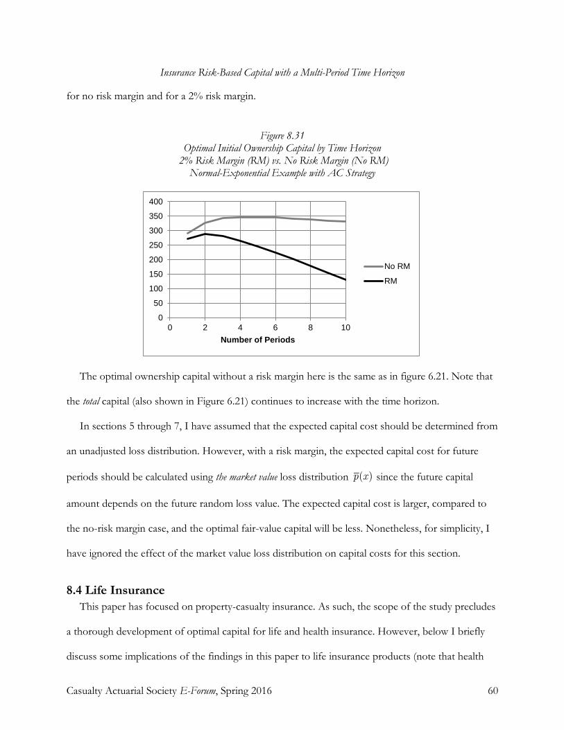
Insurance Risk-Based Capital with a Multi-Period Time Horizon
Casualty Actuarial Society E-Forum, Spring 2016 60
for no risk margin and for a 2% risk margin.
Figure 8.31 Optimal Initial Ownership Capital by Time Horizon
2% Risk Margin (RM) vs. No Risk Margin (No RM) Normal-Exponential Example with AC Strategy
The optimal ownership capital without a risk margin here is the same as in figure 6.21. Note that
the total capital (also shown in Figure 6.21) continues to increase with the time horizon.
In sections 5 through 7, I have assumed that the expected capital cost should be determined from
an unadjusted loss distribution. However, with a risk margin, the expected capital cost for future
periods should be calculated using the market value loss distribution since the future capital
amount depends on the future random loss value. The expected capital cost is larger, compared to
the no-risk margin case, and the optimal fair-value capital will be less. Nonetheless, for simplicity, I
have ignored the effect of the market value loss distribution on capital costs for this section.
8.4 Life Insurance This paper has focused on property-casualty insurance. As such, the scope of the study precludes
a thorough development of optimal capital for life and health insurance. However, below I briefly
discuss some implications of the findings in this paper to life insurance products (note that health
0
50
100
150
200
250
300
350
400
0 2 4 6 8 10Number of Periods
No RM
RM

Insurance Risk-Based Capital with a Multi-Period Time Horizon
Casualty Actuarial Society E-Forum, Spring 2016 61
insurance is similar to property-casualty insurance in that policy terms are short and there are few
embedded options).
Life Insurance Liability Risk
Generally, for life insurance the risk of losses being higher than expected is low due to the lack
of correlation between claims from separate policies. There is some chance of default from losses
occurring earlier than expected (e.g., whole life insurance) or later than expected (e.g., annuities). The
risk of default for the amount of claims and their timing can be addressed by the techniques
presented in the earlier sections. Life claims risk has a different stochastic process than long-
duration losses, since the periodic indemnity amounts are fixed but the horizon is stochastic. The
process is not Markovian, since if more/fewer insureds die, then the probability of future deaths
changes for the insured population.
Embedded Policyholder Options
A major source of risk for life insurers is the nature of the embedded options in policy contracts.
These are not usually present for property-casualty insurance. For example, life policyholders may
stop paying premiums or they may add coverage after the policy has been in force; policyholders
may be able to make loans at favorable terms; the policy may have other investment guarantees. The
effect of any of these depends on policyholder behavior. Note that some policy features may not
remain after the insurer becomes insolvent and is under conservatorship. Moreover, the policy
features that create default risk have value to the policyholder, which should be incorporated into
the consumer value in the optimal capital calculation.
Capital Funding Strategies
Notwithstanding the above differences between life and property-casualty insurance, the capital
funding strategies available to life insurers are the same as for property-casualty insurers. The

Insurance Risk-Based Capital with a Multi-Period Time Horizon
Casualty Actuarial Society E-Forum, Spring 2016 62
availability and cost of external capital will also be similar. These factors will have parallel impacts on
the amount of capital needed for life insurers. Also, modeling the asset risk will be similar, since
both types of insurers have the same categories of investments in their portfolios.
9. MULTI-PERIOD ASSET RISK
The preceding results for risky losses can be extended to the case where assets are risky. Here I
develop a method for integrating asset risk into the model and show some basic results for the AC
strategy.
I start with a treatment of asset risk in a one-period model that differs from the method in
EBRM. In that analysis, I assumed the certainty-equivalent ending value of risky assets equaled the
terminal value of the assets as if they were invested in risk-free securities. A better assumption is that
the CE value of the risky assets equals their unadjusted expected ending value minus a quantity
(called the risk premium in financial economics) that mirrors the risk value (as defined in section 2.23)
for losses. The results from this analysis are consistent with standard finance techniques for
optimizing an individual’s investment portfolio.42
9.1 One-Period Joint Loss and Asset Model For one period, where both the loss and the ending asset amount are random, the CE expected
default value is
. (9.11)
Here v represents the difference between the loss and available asset values for all combinations
42 See Bodie, Kane and Marcus [2014], chapter 6.
Insurance Risk-Based Capital with a Multi-Period Time Horizon
Casualty Actuarial Society E-Forum, Spring 2016 63
of loss and asset values that produce v, with being the CE probability of v occurring. The
expression for the unadjusted expected default D is similar to that equation 9.11, with the
unadjusted probability p(v) replacing .
Assume that the insurer’s assets consist of riskless securities having a zero return, as specified in
section 4.1, as well as an amount of risky assets AR with an expected (market) rate of return per
period. The risky assets are diversified and have the same standard deviation (SD) of return as
the market rate of return. Thus, if the insurer’s ending asset value has a SD of , then its
expected return amount is , which equals the asset risk SD times the Sharpe
ratio.43 Notice that, although the Sharpe ratio is commonly applied to stock market risk, it can also
characterize bond market risk: the expected return on a long-term bond will normally exceed that of
a short-term Treasury note; meanwhile the bond value has a positive volatility due to potential
interest rate fluctuations.
The variance of v, or the total variance, is , where is the loss
variance and represents the correlation between loss and asset values.44 Also assume that the
insurer maintains a constant asset risk as it changes its capital amount, so that additions and
withdrawals are in riskless assets.
In equation 9.11 (either the CE or unadjusted version), the expected default amount can be
43 The ratio of the expected excess return (over the risk-free rate) on a security to the standard deviation of the return is
known as the Sharpe ratio. Here the risk-free rate is assumed to be zero, so the Sharpe ratio is simply equal to . 44 For some insurance products that depend on investment performance (such as embedded options in life insurance and property-casualty products where the market value of losses depend on interest rates), the co-variation with losses may be more complex than we can represent with a simple correlation coefficient. Thus, more extensive modeling may be required for a practical application.
Insurance Risk-Based Capital with a Multi-Period Time Horizon
Casualty Actuarial Society E-Forum, Spring 2016 64
obtained by assuming that the asset risk is zero and the original loss distribution is replaced by an
alternative loss distribution that produces the same default amounts with the same probabilities as
the joint asset and loss distribution. Call the alternative loss variable the augmented loss. Since the
expected ending asset amount (prior to paying the loss) is greater than the initial value by the
expected return ER, the expected augmented loss, denoted by , is reduced by this amount; thus
. Accordingly, the augmented loss has mean and standard deviation .
Since the sum of two jointly distributed normal random variables is normal, if both the loss and
ending asset amounts are normally distributed, then the augmented loss variable is also normal. If
the asset and loss variables are not normal, then the augmented loss technique will produce
approximate results. The subsequent analysis in this section assumes joint normality for the two
variables.
The expected certainty-equivalent default calculation is the same as that of a risky loss with mean
and variance , together with riskless assets. To illustrate, assume that policyholder risk
aversion is based on exponential utility. We have (from section 4.22), and
. Thus the certainty-equivalent expected augmented loss is
. (9.12)
The quantity denotes the asset risk premium. In finance this represents
the amount by which the expected return is reduced to produce the CE ending value of the assets. If
the ending asset values and losses are statistically independent, then = 0, giving
and .
Insurance Risk-Based Capital with a Multi-Period Time Horizon
Casualty Actuarial Society E-Forum, Spring 2016 65
Using the augmented loss and total variance, the optimal capital for an insurer with both asset
and loss risk can be determined in the same way that we calculate the optimal capital for an insurer
with riskless assets in a one-period model. By subtracting the optimal joint capital from the optimal
capital for riskless assets, we get the implied optimal amount of capital for the risky assets.
Because the expected return on risky assets is positive, including some risky assets in the insurer’s
investment portfolio can reduce the solvency cost compared to that from a riskless portfolio. To
illustrate this, we use the basic example from section 5.3. Suppose that, instead of riskless assets, the
insurer now has AR = 50 units of risky assets with the remainder in risk-free securities. The market
expected return is = 5% with a volatility of = 20% and the assets are uncorrelated with
losses. Thus, the insurer’s asset risk is = 10 = 0.2(50), the expected return amount is ER = 2.5
= 50(0.05), the risk premium is RP = 0.50 = 0.01(10)2/2 and the total risk is = 100.50. Equation
9.12 gives = 1048 = 1050 – 2.5 + 0.5. The optimal capital is then 291.02, which is less than the
291.62 with no asset risk. The solvency cost with the risky assets is 6.6097, which is also less the
6.6177 for riskless assets. In this case, the optimal capital for asset risk is negative: –0.60 = 291.02 –
291.62. This example shows that a moderate amount of asset risk can actually improve policyholder
welfare: a situation akin to an individual benefitting from having an investment portfolio containing
some risky securities.
As the amount of risky assets increases, the expected return increases linearly with , but the
risk premium increases with its square. Consequently, the beneficial effect of the expected return will
vanish if the asset risk is too high. Also, the asset risk is mitigated by its combination with the loss
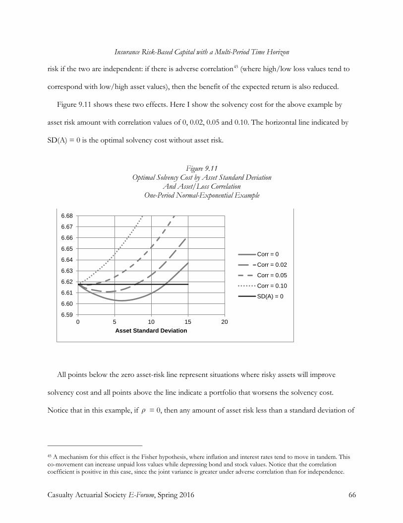
Insurance Risk-Based Capital with a Multi-Period Time Horizon
Casualty Actuarial Society E-Forum, Spring 2016 66
risk if the two are independent: if there is adverse correlation45 (where high/low loss values tend to
correspond with low/high asset values), then the benefit of the expected return is also reduced.
Figure 9.11 shows these two effects. Here I show the solvency cost for the above example by
asset risk amount with correlation values of 0, 0.02, 0.05 and 0.10. The horizontal line indicated by
SD(A) = 0 is the optimal solvency cost without asset risk.
Figure 9.11 Optimal Solvency Cost by Asset Standard Deviation
And Asset/Loss Correlation One-Period Normal-Exponential Example
All points below the zero asset-risk line represent situations where risky assets will improve
solvency cost and all points above the line indicate a portfolio that worsens the solvency cost.
Notice that in this example, if = 0, then any amount of asset risk less than a standard deviation of
45 A mechanism for this effect is the Fisher hypothesis, where inflation and interest rates tend to move in tandem. This co-movement can increase unpaid loss values while depressing bond and stock values. Notice that the correlation coefficient is positive in this case, since the joint variance is greater under adverse correlation than for independence.
6.59
6.60
6.61
6.62
6.63
6.64
6.65
6.66
6.67
6.68
0 5 10 15 20Asset Standard Deviation
Corr = 0
Corr = 0.02
Corr = 0.05
Corr = 0.10
SD(A) = 0

Insurance Risk-Based Capital with a Multi-Period Time Horizon
Casualty Actuarial Society E-Forum, Spring 2016 67
about 12 (i.e., risky assets are less than about 5% of the 1291 in total assets) will improve the
solvency cost. If the asset SD is 5.95, the optimal solvency cost is attained. Also notice that if the
asset/loss correlation is above approximately 0.06, then no amount of risky assets will improve the
solvency cost.
Although a small amount of asset risk is optimal in this example, the solvency cost is not far from
optimal if asset risk is moderately higher. For example, if the insurer has risky assets with a 40 SD,
the optimal solvency cost is 7.08, which is 0.46 greater than the zero asset-risk optimum of 6.62.
However, the difference represents only about 0.05% of the expected loss, so this reduction of value
to the policyholder may not be material in a practical setting. The optimal capital for this case is
311.34, which is greater than the 291.62 with no asset risk; the 19.71 difference represents the
amount of capital needed for asset risk.
For a one-period insurer model, if the assets are bonds whose market values have a low
correlation with the insurance losses, the above analysis shows that under a normal (positive-
sloping) yield curve, the optimal portfolio will have a duration to maturity that exceeds a single
period. Thus, in assessing capital adequacy, the standard actuarial technique of matching asset and
liability durations may not produce optimal results.
9.2 Multi-Period AC Joint Loss-Asset Model Extending the one-period joint loss-asset model to two or more periods is relatively
straightforward as long as the asset risk can be incorporated into the loss as in equation 9.12. If not,
a more complex numerical method or simulation may be necessary.
For a single-period model, the riskless interest rate (which I have assumed to be zero) is known at
the beginning of the period. However, for more than one period, the future interest rate will vary
randomly, with a mean of zero. I assume that the distribution of asset returns exceeding the risk-free

Insurance Risk-Based Capital with a Multi-Period Time Horizon
Casualty Actuarial Society E-Forum, Spring 2016 68
rate is independent of the level of the rate. Thus, the certainty-equivalent expected default values in
equation 9.12 and their counterparts for multiple periods will be the same as if the future riskless
rates were fixed at the initial one-period value. The present value of the expected CE default and the
expected capital costs (see section 8.2) can be determined by using the expected risk-free rate,46
which is zero for the simplified model in this section.
For longer horizons, joint loss-asset risk is not quite parallel to the case of multi-period risky
losses. The loss value will continue to evolve if technical solvency occurs at the end of the first
period, as in the loss-only model. However, with risky assets, if the insurer becomes technically
insolvent after the first period, the asset risk will drop to virtually zero since the insurer will enter
conservatorship shortly after becoming technically insolvent. As discussed in section 3.2, the asset
portfolio will be converted to an essentially riskless one by the conservator. For simplicity, assume
that the investment portfolio is immediately converted to riskless assets upon technical insolvency.
We also maintain the constant asset-risk assumption from the one-period model: if the insurer
remains solvent, the asset portfolio retains the same risk as the size of the portfolio changes.
Therefore, the optimal capital calculation under the joint loss-asset model is the same as with the
loss-only model having the total risk , except that (1) the available assets are greater by the
amount of the expected return on assets ER and (2) the CE technical default amount is based on
only the loss risk .
To illustrate long-horizon asset-risk capital, we can extend the one-period example from section
9.1 to the range of one to ten periods, using the AC capital strategy. Here the asset risk is 10, 20 or
46 In theory, the best rate for discounting these expected cash flows is the risk-free spot yield matching the length of the cash flow. With a normal yield curve, the spot yield for several periods will be greater than that of a single period. Although I have ignored this feature in developing the basic multi-period model, it can easily be incorporated into a practical application.
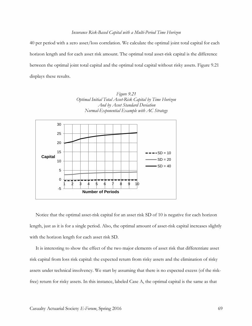
Insurance Risk-Based Capital with a Multi-Period Time Horizon
Casualty Actuarial Society E-Forum, Spring 2016 69
40 per period with a zero asset/loss correlation. We calculate the optimal joint total capital for each
horizon length and for each asset risk amount. The optimal total asset-risk capital is the difference
between the optimal joint total capital and the optimal total capital without risky assets. Figure 9.21
displays these results.
Figure 9.21 Optimal Initial Total Asset-Risk Capital by Time Horizon
And by Asset Standard Deviation Normal-Exponential Example with AC Strategy
Notice that the optimal asset-risk capital for an asset risk SD of 10 is negative for each horizon
length, just as it is for a single period. Also, the optimal amount of asset-risk capital increases slightly
with the horizon length for each asset risk SD.
It is interesting to show the effect of the two major elements of asset risk that differentiate asset
risk capital from loss risk capital: the expected return from risky assets and the elimination of risky
assets under technical insolvency. We start by assuming that there is no expected excess (of the risk-
free) return for risky assets. In this instance, labeled Case A, the optimal capital is the same as that
-5
0
5
10
15
20
25
30
1 2 3 4 5 6 7 8 9 10
Capital
Number of Periods
SD = 10
SD = 20
SD = 40
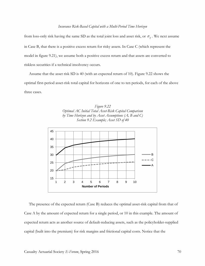
Insurance Risk-Based Capital with a Multi-Period Time Horizon
Casualty Actuarial Society E-Forum, Spring 2016 70
from loss-only risk having the same SD as the total joint loss and asset risk, or . We next assume
in Case B, that there is a positive excess return for risky assets. In Case C (which represent the
model in figure 9.21), we assume both a positive excess return and that assets are converted to
riskless securities if a technical insolvency occurs.
Assume that the asset risk SD is 40 (with an expected return of 10). Figure 9.22 shows the
optimal first-period asset-risk total capital for horizons of one to ten periods, for each of the above
three cases.
Figure 9.22 Optimal AC Initial Total Asset-Risk Capital Comparison by Time Horizon and by Asset Assumptions (A, B and C)
Section 9.2 Example; Asset SD of 40
The presence of the expected return (Case B) reduces the optimal asset-risk capital from that of
Case A by the amount of expected return for a single period, or 10 in this example. The amount of
expected return acts as another source of default-reducing assets, such as the policyholder-supplied
capital (built into the premium) for risk margins and frictional capital costs. Notice that the
15
20
25
30
35
40
45
1 2 3 4 5 6 7 8 9 10Number of Periods
B
C
A

Insurance Risk-Based Capital with a Multi-Period Time Horizon
Casualty Actuarial Society E-Forum, Spring 2016 71
policyholder-supplied capital is provided only once, at the time the premium is written, covering all
subsequent periods. In contrast, the expected return effectively provides added capital for each
period on an ongoing basis as long as the insurer is solvent and maintains the asset portfolio.
Eliminating asset risk when insolvent (Case C) reduces the asset-risk capital further for multi-
period horizons, as long as the amount of asset risk is greater than the optimal amount (an SD of
5.95 per period). If the asset risk is lower than the optimal amount, then the elimination of asset risk
when insolvent will slightly increase the optimal asset-risk capital for each period.
Insurance Risk-Based Capital with a Multi-Period Time Horizon
Casualty Actuarial Society E-Forum, Spring 2016 72
10. CONCLUSION
The purpose of this study is to determine, in principle, the risk-based capital for multi-period
insurance losses and assets. Using basic economic concepts central to insurance, I have shown how
to find the optimal multi-period capital amount without arbitrarily choosing which risk measure
(e.g., VaR, TVaR and others) and time horizon model (one-year vs. runoff) should be used. The
analysis gives proper weight to volatility in each period and incorporates important constraints, such
as conservatorship under technical insolvency and the ability to raise capital externally. Much of this
undertaking is new territory. In particular, the notions of policyholder risk preferences and dynamic
capital strategies may be unfamiliar to an actuarial audience. While falling short of a full practical
application, I have provided numerical examples to illustrate how the concepts might be applied if
the underlying parameters are known.
The major qualitative results of this paper are summarized in section 1.1. Perhaps the chief
among them are: (1) the optimal capital for long-horizon losses depends on both the annual loss
volatility and the ultimate loss volatility, and will be greater than optimal capital based on the annual
volatility, and (2) optimal capital for any horizon depends on the insurer’s ability to raise capital, and
its cost of raising capital. Analyzing the first relationship is largely a technical actuarial exercise, while
analyzing the second involves understanding an insurer’s connections to capital markets, ownership
structure and internal information processes.
Knowing the optimal capital provides the basis for applications in product pricing, corporate
governance and regulation. Due to the many variables involved, optimizing capital for multi-period
insurance can be rather complicated and perhaps daunting. However, as shown here, starting from a
basic one-period model, the requisite multi-period model can be assembled step-by-step to produce
useful results. More extensive modeling with additional elements can be accomplished using

Insurance Risk-Based Capital with a Multi-Period Time Horizon
Casualty Actuarial Society E-Forum, Spring 2016 73
simulation techniques.
The analysis in this paper has identified some important factors relevant to multi-period risk that
are not commonly considered in setting capital standards for insurance: capital funding strategies,
the cost of raising external capital, the capitalization interval, policy term, ownership structure and
the effect of conservatorship. These topics provide a fertile source for future research.
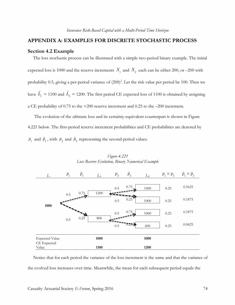
Insurance Risk-Based Capital with a Multi-Period Time Horizon
Casualty Actuarial Society E-Forum, Spring 2016 74
APPENDIX A: EXAMPLES FOR DISCRETE STOCHASTIC PROCESS
Section 4.2 Example The loss stochastic process can be illustrated with a simple two-period binary example. The initial
expected loss is 1000 and the reserve increments and each can be either 200, or –200 with
probability 0.5, giving a per-period variance of (200)2. Let the risk value per period be 100. Then we
have = 1100 and = 1200. The first period CE expected loss of 1100 is obtained by assigning
a CE probability of 0.75 to the +200 reserve increment and 0.25 to the –200 increment.
The evolution of the ultimate loss and its certainty-equivalent counterpart is shown in Figure
4.221 below. The first-period reserve increment probabilities and CE probabilities are denoted by
and , with and representing the second-period values.
Figure 4.221
Loss Reserve Evolution, Binary Numerical Example
L L1 L2
0.5 0.75 1400 0.25 0.5625
0.5 0.75 1200
0.5 0.25 1000 0.25 0.1875
1000
0.5 0.75 1000 0.25 0.1875
0.5 0.25 800
0.5 0.25 600 0.25 0.0625
Expected Value 1000 1000
CE Expected Value
1100
1200
Notice that for each period the variance of the loss increment is the same and that the variance of
the evolved loss increases over time. Meanwhile, the mean for each subsequent period equals the
Insurance Risk-Based Capital with a Multi-Period Time Horizon
Casualty Actuarial Society E-Forum, Spring 2016 75
value of the loss from the prior period: for instance, if L1 becomes 1200 at the end of period 1, then
1200 is the mean for period 2. The CE expected value of the second-period loss conditional on the
emerged 1200 amount is 1200 plus the 100 risk value for the second period, or 1300.
Section 5.1 Example Assume that the expected loss is 1000 and increments for each period range from
–400 to 400 in steps of 50; the corresponding loss probabilities are generated by a binomial
distribution having a base probability 0.5 with 16 trials. Thus the probability of a 400 increment is
(0.5)16, the probability of a 350 increment is 16(0.5)16, and so forth. The expected value of the
increments is zero and the variance is (100)2. For the parallel CE stochastic loss process, assume that
the base probability is 0.625, giving a higher subjective likelihood of larger increments: the
probability of a 400 increment is (0.625)16 = 0.00054 and the probability of a 350 increment is
16(0.625)15(0.375) = 0.00520. The CE expected value of the increment is 100, so the CE expected
loss increases by a risk value of 100 each period.
Now suppose that initial assets are 1300, so a technical insolvency occurs if the first-period loss is
either 1350 or 1400 (the maximum possible loss). When the technical insolvency occurs, the assets
remain fixed at 1300, but the loss can still develop for one more period. Consequently, if the first-
period loss is 1350, its value at the end of the second period is one of {1350 – 400, 1350 – 350, ,
1350 + 400}, or {950, 1000, , 1750}. However, only the amounts {1350, 1400, , 1750} will
produce a default when the loss is settled at the end of the second period. The respective CE
probabilities for these amounts are {0.11718, 0.17361, , 0.00054}. Weighting the possible default
amounts by their occurrence probabilities gives 152.59, the conditional CED given that the 1350
loss amount occurs.
For the 1400 first-period loss, the range of its possible second-period values that produce an
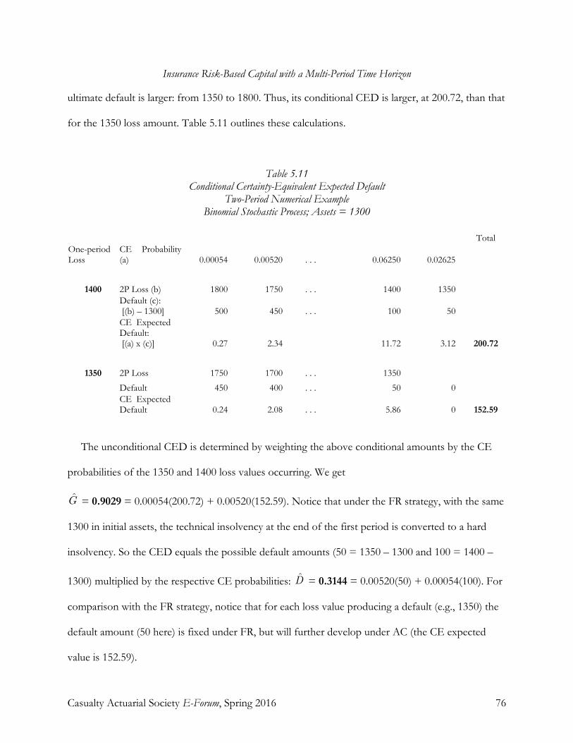
Insurance Risk-Based Capital with a Multi-Period Time Horizon
Casualty Actuarial Society E-Forum, Spring 2016 76
ultimate default is larger: from 1350 to 1800. Thus, its conditional CED is larger, at 200.72, than that
for the 1350 loss amount. Table 5.11 outlines these calculations.
Table 5.11 Conditional Certainty-Equivalent Expected Default
Two-Period Numerical Example Binomial Stochastic Process; Assets = 1300
Total One-period Loss
CE Probability (a) 0.00054 0.00520 . . . 0.06250 0.02625
1400 2P Loss (b) 1800 1750 . . . 1400 1350
Default (c): [(b) – 1300] 500 450 . . . 100 50
CE Expected Default: [(a) x (c)] 0.27 2.34 11.72 3.12 200.72
1350 2P Loss 1750 1700 . . . 1350
Default 450 400 . . . 50 0
CE Expected Default 0.24 2.08 . . . 5.86 0 152.59
The unconditional CED is determined by weighting the above conditional amounts by the CE
probabilities of the 1350 and 1400 loss values occurring. We get
= 0.9029 = 0.00054(200.72) + 0.00520(152.59). Notice that under the FR strategy, with the same
1300 in initial assets, the technical insolvency at the end of the first period is converted to a hard
insolvency. So the CED equals the possible default amounts (50 = 1350 – 1300 and 100 = 1400 –
1300) multiplied by the respective CE probabilities: = 0.3144 = 0.00520(50) + 0.00054(100). For
comparison with the FR strategy, notice that for each loss value producing a default (e.g., 1350) the
default amount (50 here) is fixed under FR, but will further develop under AC (the CE expected
value is 152.59).
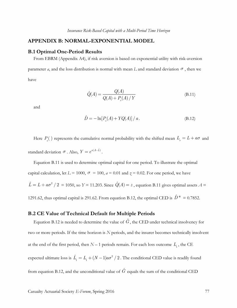
Insurance Risk-Based Capital with a Multi-Period Time Horizon
Casualty Actuarial Society E-Forum, Spring 2016 77
APPENDIX B: NORMAL-EXPONENTIAL MODEL
B.1 Optimal One-Period Results From EBRM (Appendix A4), if risk aversion is based on exponential utility with risk-aversion
parameter a, and the loss distribution is normal with mean L and standard deviation , then we
have
(B.11)
and
. (B.12)
Here represents the cumulative normal probability with the shifted mean and
standard deviation . Also, .
Equation B.11 is used to determine optimal capital for one period. To illustrate the optimal
capital calculation, let L = 1000, = 100, a = 0.01 and z = 0.02. For one period, we have
= 1050, so Y = 11.203. Since , equation B.11 gives optimal assets A =
1291.62, thus optimal capital is 291.62. From equation B.12, the optimal CED is = 0.7852.
B.2 CE Value of Technical Default for Multiple Periods Equation B.12 is needed to determine the value of , the CED under technical insolvency for
two or more periods. If the time horizon is N periods, and the insurer becomes technically insolvent
at the end of the first period, then N – 1 periods remain. For each loss outcome , the CE
expected ultimate loss is . The conditional CED value is readily found
from equation B.12, and the unconditional value of equals the sum of the conditional CED
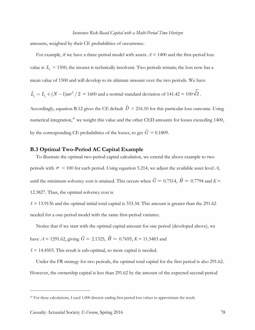
Insurance Risk-Based Capital with a Multi-Period Time Horizon
Casualty Actuarial Society E-Forum, Spring 2016 78
amounts, weighted by their CE probabilities of occurrence.
For example, if we have a three-period model with assets A = 1400 and the first-period loss
value is = 1500, the insurer is technically insolvent. Two periods remain; the loss now has a
mean value of 1500 and will develop to its ultimate amount over the two periods. We have
= 1600 and a normal standard deviation of 141.42 = 100 .
Accordingly, equation B.12 gives the CE default = 216.10 for this particular loss outcome. Using
numerical integration,47 we weight this value and the other CED amounts for losses exceeding 1400,
by the corresponding CE probabilities of the losses, to get = 0.1809.
B.3 Optimal Two-Period AC Capital Example To illustrate the optimal two-period capital calculation, we extend the above example to two
periods with = 100 for each period. Using equation 5.214, we adjust the available asset level A,
until the minimum solvency cost is attained. This occurs when 0.7514, 0.7794 and K =
12.3827. Thus, the optimal solvency cost is
S = 13.9136 and the optimal initial total capital is 333.34. This amount is greater than the 291.62
needed for a one-period model with the same first-period variance.
Notice that if we start with the optimal capital amount for one period (developed above), we
have A = 1291.62, giving 2.1325, 0.7695, K = 11.5483 and
S = 14.4503. This result is sub-optimal, so more capital is needed.
Under the FR strategy for two periods, the optimal total capital for the first period is also 291.62.
However, the ownership capital is less than 291.62 by the amount of the expected second-period
47 For these calculations, I used 1,000 discrete ending first-period loss values to approximate the result.

Insurance Risk-Based Capital with a Multi-Period Time Horizon
Casualty Actuarial Society E-Forum, Spring 2016 79
capital cost (which is policyholder-supplied capital contained in the premium) of = 5.8325, so
the first-period OC equals 285.79. The optimal solvency cost is 13.1187 = 2(0.7852) + 5.8325+
0.02(285.79).
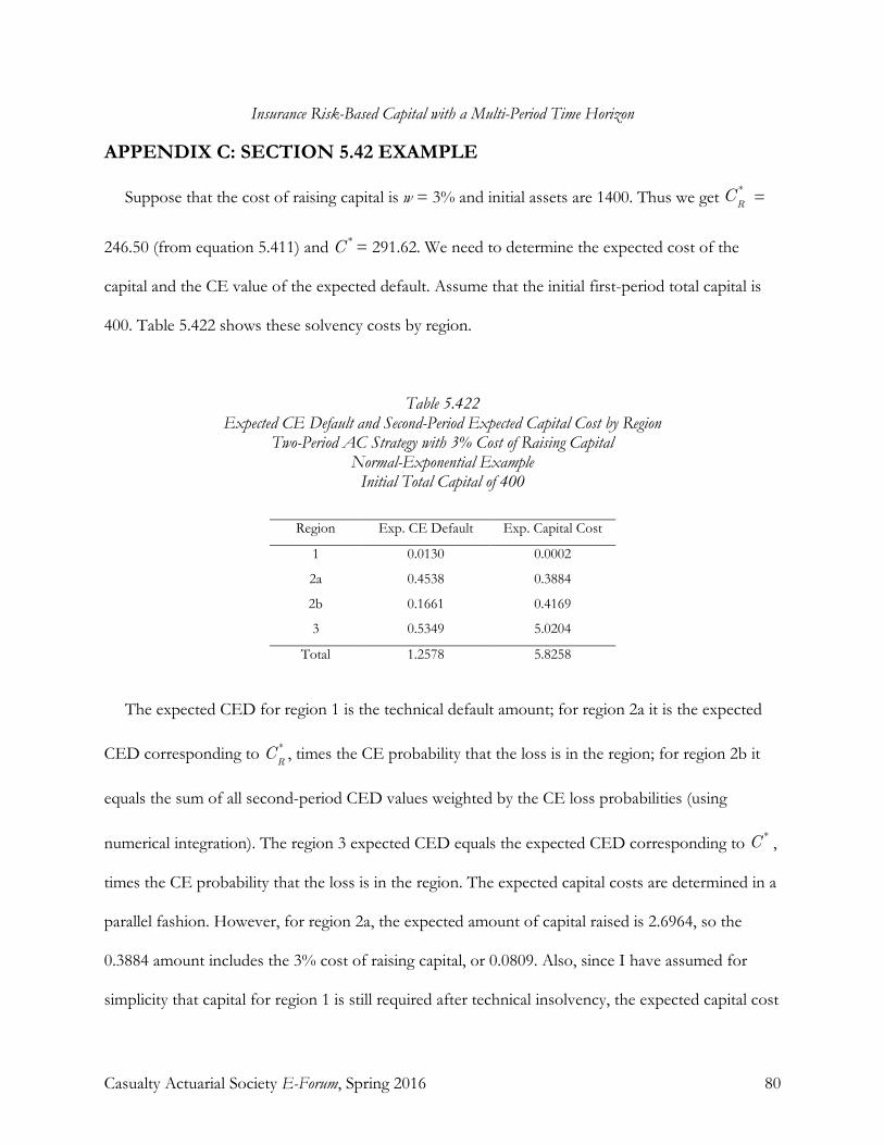
Insurance Risk-Based Capital with a Multi-Period Time Horizon
Casualty Actuarial Society E-Forum, Spring 2016 80
APPENDIX C: SECTION 5.42 EXAMPLE
Suppose that the cost of raising capital is w = 3% and initial assets are 1400. Thus we get =
246.50 (from equation 5.411) and = 291.62. We need to determine the expected cost of the
capital and the CE value of the expected default. Assume that the initial first-period total capital is
400. Table 5.422 shows these solvency costs by region.
Table 5.422 Expected CE Default and Second-Period Expected Capital Cost by Region
Two-Period AC Strategy with 3% Cost of Raising Capital Normal-Exponential Example
Initial Total Capital of 400
Region Exp. CE Default Exp. Capital Cost
1 0.0130 0.0002
2a 0.4538 0.3884
2b 0.1661 0.4169
3 0.5349 5.0204
Total 1.2578 5.8258
The expected CED for region 1 is the technical default amount; for region 2a it is the expected
CED corresponding to , times the CE probability that the loss is in the region; for region 2b it
equals the sum of all second-period CED values weighted by the CE loss probabilities (using
numerical integration). The region 3 expected CED equals the expected CED corresponding to ,
times the CE probability that the loss is in the region. The expected capital costs are determined in a
parallel fashion. However, for region 2a, the expected amount of capital raised is 2.6964, so the
0.3884 amount includes the 3% cost of raising capital, or 0.0809. Also, since I have assumed for
simplicity that capital for region 1 is still required after technical insolvency, the expected capital cost
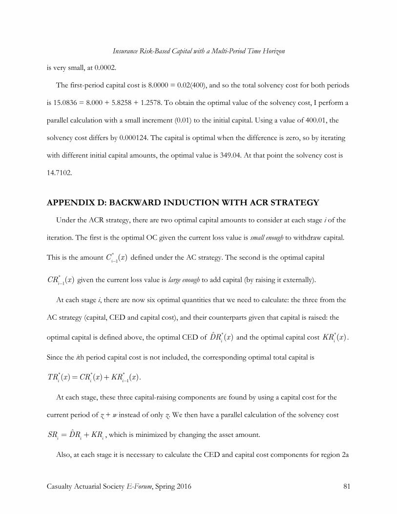
Insurance Risk-Based Capital with a Multi-Period Time Horizon
Casualty Actuarial Society E-Forum, Spring 2016 81
is very small, at 0.0002.
The first-period capital cost is 8.0000 = 0.02(400), and so the total solvency cost for both periods
is 15.0836 = 8.000 + 5.8258 + 1.2578. To obtain the optimal value of the solvency cost, I perform a
parallel calculation with a small increment (0.01) to the initial capital. Using a value of 400.01, the
solvency cost differs by 0.000124. The capital is optimal when the difference is zero, so by iterating
with different initial capital amounts, the optimal value is 349.04. At that point the solvency cost is
14.7102.
APPENDIX D: BACKWARD INDUCTION WITH ACR STRATEGY
Under the ACR strategy, there are two optimal capital amounts to consider at each stage i of the
iteration. The first is the optimal OC given the current loss value is small enough to withdraw capital.
This is the amount defined under the AC strategy. The second is the optimal capital
given the current loss value is large enough to add capital (by raising it externally).
At each stage i, there are now six optimal quantities that we need to calculate: the three from the
AC strategy (capital, CED and capital cost), and their counterparts given that capital is raised: the
optimal capital is defined above, the optimal CED of and the optimal capital cost .
Since the ith period capital cost is not included, the corresponding optimal total capital is
.
At each stage, these three capital-raising components are found by using a capital cost for the
current period of z + w instead of only z. We then have a parallel calculation of the solvency cost
, which is minimized by changing the asset amount.
Also, at each stage it is necessary to calculate the CED and capital cost components for region 2a

Insurance Risk-Based Capital with a Multi-Period Time Horizon
Casualty Actuarial Society E-Forum, Spring 2016 82
(where capital is neither raised nor withdrawn) by numerical integration: we vary the capital amount
in this region and weight the results by the corresponding loss probabilities.
To illustrate this process, I use the normal-exponential example with a 3% CRC. For one period
we have the key variables = 291.62, = 0.7852, = 5.8325,
= 246.50, = 2.2839 and = 4.301. To obtain the optimal two-period value , we
start with an arbitrary initial capital amount (the optimal one-period capital of 291.62 is a good start)
and calculate the solvency cost as in Appendix C. This is done by adding the CED and capital cost
components for the four regions of first-period loss outcomes (see section 5.42). This calculation
uses the above six key variables. We perform a parallel calculation with the capital increased by a
small amount (say, 0.001). We adjust the capital amount (and its incremental counterpart) until the
difference between the incremental and the original solvency costs is zero. This occurs when A =
1349.04 and = 14.7102, giving = 349.04, = 343.16,
= 1.8536 and = 12.8566.
We next do a second calculation where the first period capital cost is z + w = 0.05. This provides
the optimal values of the key variables for the case where capital is raised after the first period of a
three-period horizon (we are preparing for the next stage of the induction procedure). Here we get
= 301.00, = 3.2764 and
= 12.0567.
We continue the induction process to get the optimal key variables for longer horizons.
ACKNOWLEDGMENTS
In 2011, the American Academy of Actuaries committee sought help from the Casualty Actuarial
Insurance Risk-Based Capital with a Multi-Period Time Horizon
Casualty Actuarial Society E-Forum, Spring 2016 83
Society (CAS) in preparing risk-based capital proposals for the National Association of Insurance
Commissioners. I joined the CAS RBC Dependency and Correlation Working Party, led by Allan
Kaufman. As my contribution to this effort, I began a project to determine the best solvency risk
measure for property-casualty insurers. The paper An Economic Basis for Property-Casualty Insurance
Risk-Based Capital Measurement was the product of that effort. I also undertook a second project, to
determine risk-based capital for multi-period insurance. This assignment greatly expanded my earlier
work, and this paper is the result. I am deeply thankful for Allan’s patient stewardship in guiding me
along this lengthy learning process. His innumerable astute comments, sharp critique and editorial
suggestions were invaluable; they forced me to explain results more clearly — the paper is much
better for his involvement.
REFERENCES
[1] A.M. Best, 2003, “The Treatment of Surplus Notes and Trust-Preferred Securities in the Financial Strength Ratings of Insurance Companies”, A.M. Best Special Report
[2] Bharucha-Reid, A. T. Elements of the Theory of Markov Processes and Their Applications. New York: McGraw-Hill, 1960.
[3] Bodie, Zvi, Alex Kane and Alan Marcus, Investments, 10th edition. New York: McGraw Hill/Irwin, 2014 [4] Butsic, R., 1988, Determining the Proper Interest Rate for Loss Reserve Discounting: An Economic Approach,
Casualty Actuarial Society Discussion Paper Program. 147-170 [5] Butsic, R., An Economic Basis for Property-Casualty Insurance Risk-Based Capital Measurement, Casualty
Actuarial Society E-Forum, Summer 2013 [6] California Liquidation Office 2014 Annual Report [7] Cummins, J. David and Danzon, Patricia M., Price, Financial Quality, and Capital Flows in Insurance Markets,
Journal Of Financial Intermediation 6, 3–38 (1997) [8] European Parliament Directive 2009/138/EC (Solvency II) [9] Han, Zhongxian; Gau, Wu-Chyuan; 2008, Estimation of loss reserves with lognormal development factors;
Insurance.- Amsterdam: North Holland Publ. Co, ISSN 0167-6687, ZDB-ID 8864x. - Vol. 42.2008, 1, p. 389-395 [10] Harrington, Scott E., and Niehaus, Greg, Capital Structure Decisions in the Insurance Industry: Stocks versus
Mutuals, Journal of Financial Services Research, February 2002, Volume 21,Issue 1-pp 145-163 [11] Lowe, Stephen, François Morin, and Dean Swallow, Risk Horizon and the Measurement of Economic Capital for General
Insurers, Towers Watson, 2011. [12] Myers, Stewart C. and Nicholas S. Majluf (1984), Corporate Financing and Investment Decisions When Firms
Have Information that Investors Do Not Have, Journal of Financial Economics 13 (2): 187-221. [13] John von Neumann and Oskar Morgenstern, "Theory of Games and Economic Behavior", Section 15.3.1.
Princeton University Press. Third edition, 1953. (First edition, 1944.) [14] New York Liquidation Bureau 2014 Annual Report [15] Panjer, Harry H., ed., (1998) Financial Economics with Applications to Investments, Insurance, and Pensions,
Society of Actuaries. [16] Wacek, Michael G., The Path of the Ultimate Loss ratio Estimate, Casualty Actuarial Society Forum, Winter 2007

Insurance Risk-Based Capital with a Multi-Period Time Horizon
Casualty Actuarial Society E-Forum, Spring 2016 84
GLOSSARY OF ABBREVIATIONS AND NOTATION
Abbreviation Meaning Section
Defined AC Add capital (strategy) 4.5 ACR Add capital (strategy) with cost of raising capital 5.4 CE Certainty-equivalent 2.1 CED Certainty-equivalent expected default 2.1 CI Capitalization interval 7.3 CW Capital withdrawal (strategy) 4.5 EBRM Economic Basis … Risk Based Capital Measurement 1 FA Fixed assets (strategy) 4.5 FCC Frictional capital cost 2.2 FR Full recapitalization (strategy) 4.5 IFRS International Financial Reporting Standards 1 OC Ownership capital 4.4 SD Standard deviation 9.1 SH Stochastic horizon 8.1 VaR Value-at-risk 1 TVaR Tail value-at-risk 1
Variable Meaning Section Defined
a Risk aversion parameter 4.2 A Assets 2.1 AR Risky asset amount 9.1 C Capital (ownership) 4.1 CF Capital flow 4.5 CR Capital raised externally App. D D Expected default 2.1 DR Expected default if capital is raised App. D E( ) Expectation operator 4.3 EF Expected capital carried forward 5.4 ER Expected return 9.1 G Expected default under technical insolvency 5.1 H Expected default for remaining periods 5.2 i Period index 4.3 K Expected capital cost 4.3 KR Expected capital cost if capital is raised App. B L Expected loss 2.1 M Risk margin value 8.3 N Number of periods 4.1 p( ) Probability density 2.1 P( ) Cumulative probability 6.2 q Probability of period length 8.1 Q Default probability 2.2 r Risk-free interest rate 8.2

Insurance Risk-Based Capital with a Multi-Period Time Horizon
Casualty Actuarial Society E-Forum, Spring 2016 85
Market rate of return 9.1
R Expected return on capital 8.3 RP Risk premium 9.1 S Solvency cost 5.2 SR Solvency cost with capital raised externally App. D t Income tax rate 8.3 T Total capital 4.4 TR Total capital when raised externally App. D v Loss minus asset value 9.1 V Consumer value 2.2 w Cost of raising capital 5.4 x Loss or asset size 2.1 X Reserve increment 4.2 Y Ratio of successive reserve amounts 4.2 z Frictional cost of capital 2.2
Partial derivative operator 5.2 Capital increment App. B Premium 2.2 Asset/loss correlation 9.1 Standard deviation 4.2
Subscript
a Region 2a 5.4 A Assets 9.1 b Region 2b 5.4 E Ending capital 5.4 L Losses 9.1 M Market R Raising capital 5.4 t Elapsed time 4.2 T Total assets and losses 9.1
BIOGRAPHY OF THE AUTHOR
Robert P. Butsic is a retired actuary currently residing in San Francisco. He served as a member of the American Academy of Actuaries Property-Casualty Risk Based Capital Committee and is a member of the Casualty Actuarial Society’s Risk-Based Capital Dependency and Calibration Working Group. He previously worked for Fireman’s Fund Insurance and CNA Insurance. He is an Associate in the Society of Actuaries, has a B.A. in mathematics and an MBA in finance, both from the University of Chicago. He has won the Casualty Actuarial Society’s Michelbacher Award (for best Discussion Paper) five times. Since the 2008 financial crisis he has enjoyed reading economics blogs, which have contributed to the development of this paper.
Casualty Actuarial Society E-Forum, Spring 2016 1
Pitfalls of Predictive Modeling
By Ira Robbin ________________________________________________________________________ Abstract:
This paper provides an accessible account of potential pitfalls in the use of predictive models in property and casualty insurance. With a series of entertaining vignettes, it illustrates what can go wrong. The paper should leave the reader with a better appreciation of when predictive modeling is the tool of choice and when it needs to be used with caution Keywords: Predictive modeling, GLM
1. INTRODUCTION
There are many success stories featuring use of Predictive Models in Property and Casualty Insurance applications, but what does not get so widely reported are the failures: mistakes that range from subtle misinterpretations and minor miscues to unvarnished disasters. What is a Predictive Model? Some use the term in a generic way to refer to any model used to make predictions. However, others use the term in a more restrictive sense to refer only to Generalized Linear Models (GLM) and related methodologies. That is the approach taken in this paper. This article will focus on the use of the GLM family of predictive models in Property and Casualty insurance and will illustrate several pitfalls. Many of the pitfalls have nothing to do with technical aspects of model construction, but rather with false assumptions about the data or misapplications of model results.
1.1 If You Build It, They Will Come Predictive Modeling has experienced an incredible surge in popularity over the last decade.
This is due not just to the marketing appeal of the “Predictive Modeling” label, but more fundamentally to the rise of “Big Data”. The increased availability of large datasets, cheap data storage capacity, and computers capable of quickly processing large amounts of data make it feasible to apply GLMs to gain new insights and potentially reap competitive advantages. There has been a rush to jump on the bandwagon and start building models. It is in this context that models and their results have sometimes been accepted uncritically and recommendations supposedly dictated by a model have been treated as if issued by a Delphic oracle, not subject to question. The view of the author is that the models are quite useful and often are the tool of choice, but the actuary needs to be aware of the pitfalls in their construction and use.
Pitfalls of Predictive Modeling
Casualty Actuarial Society E-Forum, Spring 2016 2
1.2 Existing Literature There already are papers about pitfalls in the use of Predictive Models. In their paper,
Werner and Guven ([9]) warn against the “failure to get full buy-in from key stakeholders” and admonish analysts for not doing appropriate up-front communications. They discuss how to explain results to non-technical audiences. Kucera ([3]) gave a presentation on pitfalls that listed the challenge of getting senior management buy-in and the danger of “treating predictive modeling as a black box”. He also highlighted the problems that exist getting reliable data and the need for the IT resources to be available to implement models. The author agrees with most if not all that is said by Werner and Guven as well as by Kucera. However, their main focus is about pitfalls that could prevent a presumably sound model from gaining acceptance or that could forestall sensible model-based recommendations from being implemented. In contrast, the focus in this paper is to make modelers more clearly aware of some of the real pitfalls in the construction and use of models. These are pitfalls that could lead the unwary analyst to make a foolish or useless recommendation or lead a gullible company to implement an unprofitable strategy.
1.3 Organization of the Paper The discussion will begin in Chapter 2 with a definition of Predictive Modeling, contrasting
it with other modeling approaches used to make predictions. The basic framework for Predictive Modeling will be explained and this will lead to a summarization of the factors that determine when it will be effective.
Chapter 3 will turn to insurance applications. It will survey a range of proposed and actual uses and examine successes and challenges.
Chapter 4 consists of a series of vignettes illustrating what can go wrong.
2. PREDICTIVE MODELING
2.1 What is a Predictive Model? The term, “Predictive Model”, is itself subject to some debate. Some use it in a generic
sense to refer to any model used to make predictions. However, the usage in this paper will be that the term, “Predictive Model”, refers only to a Generalized Linear Model (GLM) or other related model. This is intended to exclude catastrophe (CAT) simulation models and Econometric time-series models. These other models use different approaches to solve
Pitfalls of Predictive Modeling
Casualty Actuarial Society E-Forum, Spring 2016 3
different types of problems. The author believes use of one term for all tends to muddle critical distinctions. In particular, GLM applications seldom explicitly consider time as a separate factor, whereas Econometric time-series models are fundamentally about the evolution of variables over time. As another point of contrast, consider GLMs are used to estimate the relativities of expected loss between different groups of customers and seldom consider the aggregate loss, but CAT models are designed to estimate portfolio loss distributions from large events given the exposure concentration of the portfolio.
Beyond the conceptual differences, in practice it was the author’s experience at large Commercial Lines insurers and reinsurers that CAT modelers, Econometric analysts, and Predictive Models worked in different departments using different software1. While this could change in the future, what the author has seen is that Predictive Modelers generally construct and run GLMs, but not CAT or Econometric analyses.
GLMs do not “predict” the future as much as they describe relations between different fields of data that existed at the time the data were gathered. GLM predictions of the future are thus forecasts predicated on the implicit assumptions that those relations will continue into the future. Only a more explicit treatment of what lies ahead can produce an explicit opinion about whether such assumptions are reasonable in any specific case.
The GLM terminology has been around since the 1970’s when Nelder and Wedderburn ([6]) unified several existing linear modeling techniques in a “generalized” construct.
2.2 GLM Predictions Construction of a GLM entails using data on attributes of individuals2 to estimate the value
of the outcome variable for each of those individuals. The process of modeling involves selecting structural relations and fitting parameters to give the best parsimonious fit of the predictions to the actual outcomes. Once the GLM has been constructed and the parameters determined, one can then employ it to use information on some of the attributes of another individual not in the original data set and “predict” the outcome for that individual.
This notion of prediction has nothing necessarily to do with peering into the future, but it
1 It is the author’s experience that employers and recruiters adhere to these distinctions in terminology. In particular there are separate ads for CAT modeling and Predictive modeling positions. 2 An individual member of the population could well be an insurance policy or an insurance claim. It could also refer to a corporation, a country, a sports team or other collective entity and the population sample is a subset of all such entities.
Pitfalls of Predictive Modeling
Casualty Actuarial Society E-Forum, Spring 2016 4
is useful nonetheless. For example, suppose I already have a GLM that predicts the amount a consumer will spend on the purchase of low-fat yogurt. If I learn you have 3 or more pair of red shoes, downloaded 5-8 songs from iTunes last month, have a credit score between 700-740, bought a low emissions car last year, and weigh between 100 and 190 pounds, then with that pre-existing GLM, I might be able to predict you are five times as likely to have purchased low-fat yogurt last week than another person chosen at random from the database. Or I could predict that a person with your attributes spent an average of $3.28 per week last year on low-fat yogurt. With another variation, I could also compute a score based on your attributes and on the basis of that score assign you to the second of five quintiles of low-fat yogurt consumption. The predictions are not foolproof: I could be wrong. Despite what all your other attributes might lead me to believe you may have an aversion to yogurt and would not be caught dead buying any.
As this example demonstrates, GLMs can be used to make predictions about:
• Relativities between individuals in the population with respect to some dependent outcome variable,
• Expected average outcomes for each individual, and
• Subgroup membership of individuals
Applications abound in marketing, advertising, politics, and other areas.
2.3 Modeling Process
2.3.1 Explanatory Variables
GLM predictions of individual outcomes are based on the values of various input variables, often called explanatory variables. The input variables could be continuous or categorical. A continuous variable can be recast as a categorical one by using a set of ranges. The ranges need not be of uniform size or have the same number of members. For example starting with the weight of an individual consumer as a continuous variable a set of five weight ranges could be defined as shown in Table 1.
While the frequencies do not have to be equal, it is desirable to avoid ranges with percentages so small that they have few representatives in the population. It will be difficult to pin down and prove statistical significance for the coefficients associated with such sparsely populated ranges.
Pitfalls of Predictive Modeling
Casualty Actuarial Society E-Forum, Spring 2016 5
Table 1
Weight Range Frequency
Less than 100 lbs. 25%
100-150 lbs. 30%
150-190 lbs. 20%
190-220 lbs. 15%
Over 220 lbs. 10%
Total 100%
Beyond ranges, one has the license to transform continuous inputs or outputs in a variety of ways that may dramatically improve the fit. Variables can be squared, raised to higher powers, and polynomial functions can be used. Log transforms are also commonly employed on continuous data such as insurance claim severity. The modeler uses diagnostics to figure out, on a statistically sound basis, just how much weight to give each transformed input variable in making the prediction. Some “explanatory” variables may be ignored in the estimation. Intuitively these are either independent of the dependent variable being predicted and so have no explanatory power, or are so closely related to a mix of other input variables that they are extraneous. The remaining variables in the model should all have weights statistically different from zero.
2.3.2 Goodness-of-fit Statistics
The modeler will examine goodness-of-fit statistics to determine how good a fit has been achieved. One such statistic is root mean square error (RMSE) where mean square error is the average square difference between the model result and the actual outcome. This can be improved by adjusting for differences in the expected variance: an error of a given magnitude that is large relative to the expected variance should penalize the model more than the same magnitude error when a much larger variance in to be anticipated. A generalization of the RMSE called the Deviance captures these effects.
Pitfalls of Predictive Modeling
Casualty Actuarial Society E-Forum, Spring 2016 6
When the outcome data are assumed to have a conditional parametric form, the best fit parameters for a given parametric structure can be found by Maximum Likelihood (MLE) techniques. For example, claim counts in each cell might be assumed to be conditionally Poisson and the structure of the model would express the Poisson parameter for a cell as a function of the explanatory variables. An error bar around the MLE parameters can be found using more advanced formulas such as the Rao-Cramer bound.
Another statistic called the lift measures how much better the model does at prediction than going with random chance. For example, using random chance to assign survey participants to quintiles of low-fat yogurt consumption would result in only 20% being correctly assigned on average. Suppose using a pre-existing model, one was able to boost the percentage of correct assignments to 50%. Then the lift is 2.5 (= .50/.20).
Another important measure of model fit is the R2 statistic. This measures the relative proportion of the total variance of the outcome that is explained by the model. An R2 of unity implies all variation has been captured by the model, but that may mean the model is tracking the noise in the data and confusing it with systematic effects.
More generally Goodness-of-fit for purposes of predictive modeling involves more than reproducing the given outcomes. It entails fitting that will lead to a model that is useful in predicting outcomes for different sets of data. So while the most basic fitting statistics measure only how closely a model fits the data, more advanced measures try to minimize the noise by implementing an Occam’s razor philosophy of modeling. This is done by using a measure of fit that penalizes use of additional variables. One such measure is the Akaike Information Criterion (AIC).
This very brief introduction to fitting statistics is not definitive or complete. It is meant to present a few commonly used metrics and make the reader aware there is a natural tension between fitting too closely and making good predictions.
2.3.3 Variable Selection
A key challenge is to select a good set of explanatory variables to use in the model. As noted by Sanche and Lonergan ([7]), “When a modeling project involves numerous variables, the actuary is confronted with the need to reduce the number of variables in order to create the model”. The tendency to load up a database with variables that are highly correlated with one another should be avoided. Later in the process the near-duplicates will need to be thrown
Pitfalls of Predictive Modeling
Casualty Actuarial Society E-Forum, Spring 2016 7
out. For example, the age of a driver is likely to be highly correlated with the number of years a driver has been licensed. Having both of those variables in a model adds duplicate information and leads to coefficients that are unstable.3 Even if the explanatory variables are not highly correlated, the model with more variables is not necessarily the better model: it may actually have less predictive power due to overfitting.
2.3.4 Overfitting
Overfitting means that a model has too many explanatory variables and the model is too complex when it does not need to be so. Some of the variables are extraneous in explaining the results because they are simply tracking the random fluctuations of the fitted data and they could be actively misleading when used to make predictions on new data. One clear sign of overfitting is the presence of one or more coefficients that are not statistically significant.
Overfitting can also be present even if all coefficients are statistically significant on the given data set. In this case, the extra variables are modeling eccentricities in the particular data set at the cost of reducing the predictive power of the model on other data sets.
2.3.5 Training Sets versus Testing Set
A frequently used “best-practice” is to train the model on a subset of the data, the training set. Then its accuracy is tested by looking at the predictions it makes on the hold-out data, the data not used in the fitting. The hold-out data is also called the testing set.
Analysis of the accuracy of fits on the testing set is important. It can quickly reveal overfitting. Testing accuracy on hold-out data is a procedural protection against the tendency to add variables that effectively model the noise. More advanced procedures such as cross-validation4 also address this problem of estimating how well the model ought to work when applied to, but not refit to, other data.
2.4 Significance and Sample Size
2.4.1 Not Enough
It is critical that there be enough points in the sample to pin down the coefficients with a sufficient degree of statistical precision. A larger sample size might be required all else being 3 As stated by Sanche and Lonergan [7], “The parameter estimates of the model are destabilized when variables are highly correlated between each other.” 4 See Hastie, Tibshirani, and Friedman [1].
Pitfalls of Predictive Modeling
Casualty Actuarial Society E-Forum, Spring 2016 8
equal if the outcome variable is relatively noisy. An outcome variable with many zeros and few large values is an example of a relatively noisy outcome. Such outcomes are common in insurance applications. Another factor that could increase the sample size is if the coefficient for a variable is of small magnitude. In that case, more trials are needed to achieve a level of confidence to reject the null hypothesis that the coefficient is zero.
2.4.2 Too Much
On the other extreme, with large sample sizes almost all differences are statistically significant. However, the differences are often not terribly relevant. The reason is that in nature null hypotheses are rarely exactly true, but are more often approximately true. The modeler should be wary of letting in variables that even though statistically significant lead to differences that are insignificant in practical terms. For example, a 0.1% difference in yogurt consumption between those having street addresses with even numbers versus those having street addresses with odd numbers may be statistically valid at the 95% level of confidence when the data base is very large, but it is of no practical consequence. Such differences also have a way of disappearing when the model is fit to new data and their presence may be regarded as a possible sign of overfitting.
Further, hypothesis tests in large samples should be conducted at substantially smaller significance levels so as to retain good power. Using the same significance levels that one would use in small samples fails to balance the costs of the two error types.
2.5 Bad Data
2.5.1 Outliers
The modeler may throw out (or cap) some unusually large input values or outcomes as “outliers”. For example someone in the training set may have purchased 1,200 cups of non-fat yogurt wholesale last week for resale at their diner, another may have grown bored with the interview and typed in 999, another may have misunderstood the question to be how many cups could they eat in a competitive eating contest and answered 150, and another may have bought 120 cups last week for their college sorority. Some of the outliers are errors, some are bad data, some are correct but in a context different from the one assumed by the modeler, and still others are extreme yet legitimate values. It is hard to decide which without burrowing into the data, but it is usually prohibitively costly or otherwise impractical to do so. Removing the outliers is usually the preferred route as it costs little and often leads to only minor increases
Pitfalls of Predictive Modeling
Casualty Actuarial Society E-Forum, Spring 2016 9
in the theoretical error. However, the modeler should investigate further if there are an unduly large number of outliers or if they cluster about any particular values.
2.5.2 Missing Data
Often there are individuals on whom the data is incomplete: we know some of the attributes for these individuals, but not all. The question the modeler faces is whether to throw out all such records in the database or attempt to fill in missing fields with likely values. For example, if 20% of the sample population refused to supply information on their credit scores, we could randomly assign credit scores by sampling the remaining 80%. We could go further and use correlations that exist in the group with more complete data to possibly do a better job of filling in the missing data. However, in concept, these fill-in approaches only work if the data is missing at random. If the attribute of having a missing credit score is strongly correlated with low-fat yogurt preference, then filling in a value for the credit score eliminates a possible source of information. In that case, it may be worthwhile to develop a model that has “missing” as its own category.
Note this sense of “filling-in” data is distinct from the auto-complete or auto-correct algorithms that start with text a user has entered and attempt to correct and complete the word. Such algorithms may have large dictionaries of words (and spelling and typing mistakes often made by users) to compare against the text entered and each additional symbol entered narrows down the search.
Related to the problem of missing data is the problem of data that is not missing, but should be. Sometimes those collecting data will fill in missing fields with default values. This might happen for instance if the company collecting the data admonishes the data collectors to fill in all fields. Strange clusters can result. For example, we might find that all data from ACME Data Collection Services, LLC is complete, but 20% of its records show a credit score of 678.
2.5.3 Misunderstood Data
The modeler should do the necessary investigation to ensure each of the variables is consistently defined across the entire data base. Problems of definition can easily crop up within a large company operating in several locations or when there are several different data suppliers. With multinational companies, one often encounters currency data that was originally drawn from mixed currency datasets but which was later converted to a common currency. It is sometimes better to keep separate databases and develop separate models for
Pitfalls of Predictive Modeling
Casualty Actuarial Society E-Forum, Spring 2016 10
each currency, but if the data is kept together the analyst should find out and verify just how the currencies were converted. A finding that consumers from country X spend twice as much on yogurt as consumers from other countries could be true or it could be an artifact of the way currencies were converted.
Categorical variables are prone to being defined differently by different data suppliers unless care is exercised to ensure the definition is implemented consistently. For example, for some of the data suppliers a “low emissions passenger vehicle” might have included diesel engine sedans since most have low emissions of carbon dioxide and carbon monoxide. Other data suppliers might have seen they have high levels of nitrous oxide emissions and put them in a different emissions class. In another example, when a company adds a new variable, it is often surprising how difficult it is for all company personnel and agents to administer it consistently. Who is a “good student” eligible for a good student discount? Does it include the first year second semester junior college student who got “A”s the first semester after getting “C”s in high school?
The modeler should try to find and fix all such inconsistencies in definition. Any remaining concerns about the data should be disclosed as they may impact how much reliance to place on the model in the real world.
2.5.3 Feeling Lucky
With a large enough set of significant variables, we run into the increasing possibility that at least one variable doesn’t truly belong and was let in only by the luck of the draw. Intuitively, if statistical significance has been defined at the 99% level, then with one hundred variables that are all statistically significant on a particular set of data, we might expect one of them has achieved its significance through luck. What that means is that its apparent significance is a false positive. Of course we can bump up the level of significance, but each such increase requires a larger sample size to declare variables are significant at that level.
2.6 Biased Samples The validity of extending predictions from a model based on one set of data to a different
set of data rests on the critical assumption that the sample used to train the model was an unbiased sample. In many cases however the sample is really a sample of convenience, data that a company has on its existing customer base, for example. Self-selection also frequently introduces bias: those who reply to a survey are often different from the general population.
Pitfalls of Predictive Modeling
Casualty Actuarial Society E-Forum, Spring 2016 11
The relevance of bias may depend critically on the application. If we know our sample of yogurt purchase preferences was obtained from people who responded to an on-line survey that provided a coupon for $5 worth of free yogurt for finishing the survey, we might find the results biased and misleading if we use it to launch a marketing campaign to lure new customers who have never tried yogurt.
Care also needs to be exercised in selecting the training set so that it is random and representative of the whole population of interest. If for example the training set is the first 1,000 surveys submitted to the company and 500 of these were collected by a survey firm that offered $5 off tickets to a NASCAR event for those completing the yogurt preference survey, our resulting model might fail on the testing set in which those who attended a NASCAR event in the last year make up 10% of the population.
In insurance applications some may treat one set of accident years (AYs) as a training set and another set of AYs as the testing set. This may provide some insight about the model, but it risks confounding time series effects with Predictive Model variable effects.
2.7 Predictions of the Future To use a Predictive Model to make predictions of the future, one is implicitly or explicitly
assuming the future will be sufficiently like the past so model predictions remain valid. This may not be such a bad assumption as far as predicted relativities are concerned. However, predictions of the future value of an absolute monetary amount should be viewed with caution. We might grant that a prediction that a consumer in the second quintile of yogurt consumption this year is likely to be in the same quintile next year. However, additional econometric assumptions are needed to arrive at a prediction that the person will spend an average of $3.79 a week next year, up from the predicted $3.28 per week spend this year.
2.8 Correlation, Causality, and Hidden Variables Statistical analysis on its own can only show whether an input is correlated to the output
variable. This does not imply a causal relation. No matter their degree of statistical significance, a deliberate change made in the inputs will not necessarily produce a change in the output. Owning a pair of red shoes may be a significant variable in predicting the purchase of low-fat yogurt, but giving red shoes to those that did not have them will not necessarily make them any more likely to make such a purchase.
Often there are hidden variables that directly impact both the input and the output. In such
Pitfalls of Predictive Modeling
Casualty Actuarial Society E-Forum, Spring 2016 12
a situation, a change in the input is telling us something about a change in the hidden variable which by extension is also causing a change in the output variable. If we consciously alter the explanatory input variable, we eliminate its relation to the underlying hidden variable and thereby eliminate its predictive power.
2.9 Art versus Science Given the same set of data, would seventy different but capable modelers, like the
translators of the Septuagint, come up with nearly the same set of variables and transformations and structural equations and thus arrive at nearly the same predictions? Or would we get seventy different training set designs, seventy different models and seventy different predictions? This would be highly undesirable. Instead it would be hoped that any capable practitioner could select a reasonable set of variables and transformations, use an appropriately random training set, and arrive at a model that would be roughly similar to one produced by another competent modeler. However, at this point there is little in the way of proof. But given the common training foundations and the sharing of best practices, it is the author’s opinion that different competent Predictive Modeling teams will arrive at roughly the same answer. Yet a more careful manager might want to give one set of data to two separate teams deliberately kept apart from each another. A large divergence in their answers would indicate the need for caution and further investigation.
.
3. PREDICTIVE MODELING IN PROPERTY CASUALTY INSURANCE
3.1 Personal Lines Predictive Modeling in Property Casualty insurance has been most widely used in pricing,
underwriting, and marketing personal insurance products such as Personal Auto and Residential. Those lines are well-suited for Predictive Modeling. There are a large number of policyholders and extensive reliable information on their attributes.
There is also extensive data on the losses. The number and size of the claims for each policyholder are known over many policy periods. There are enough losses and the losses are usually small enough that any real effects come through and are not overwhelmed by noise.
Proper analysis of all this data promises a potentially large payoff: a company with a better
Pitfalls of Predictive Modeling
Casualty Actuarial Society E-Forum, Spring 2016 13
model than its competitors might be able to find the most profitable niches, ones its competitors are unaware of. Just as valuable, it can better avoid unprofitable classes.
3.1.1 Credit Scoring and Telematics
Predictive models in Personal Auto have also been implemented using Credit Scoring and Telematics data. Credit Scoring takes items on an individual’s credit report and computes a score that is used in underwriting and pricing. Telematics uses a remote device to gather data on how an insured vehicle is actually being driven.
US State regulators and the general public have adopted increasingly negative views on the use of Credit Scoring and many states have laws restricting its use.5 McCarty ([4]) argues the use of Credit Scoring appears to unfairly penalize the poor and has a disparate adverse impact on racial minorities, recently divorced people, new immigrants, and those adhering to religions that discourage borrowing. Beyond that, the author believes most of the public finds the connection too tenuous: if I take out a new credit card at a retail store and get 20% off my purchases that day, why should I pay an extra $50 for car insurance two months later? In contrast, many accept the plausibility of territorial rating differentials: one county has higher costs than another due to greater traffic density or more expensive medical care and repair costs. So when the statistics bear that out, there is an attitude of acceptance. In the view of the author, a purely statistical connection, without a plausible causal explanation, seems much less compelling to the public.
Though the use of Telematics for Personal Auto rating is fairly new, it appears to the author to have achieved greater consumer acceptance than Credit Scoring. Several factors may explain this. First is the obvious point that acceptance of a telematics device is often coupled with a price discount. A second appealing feature is that it is the customer who makes the decision to accept a Telematics device. Finally, the author speculates that many consumers find it logical and fair that their rates should be adjusted based on data on how their vehicle is being driven.
Telematics may in fact be reducing claim costs, as drivers operate their vehicles more safely knowing the computer is recording their every move. On the other hand, those accepting a telematics device may be a biased sample of those who are extremely safe drivers to begin
5 See McCarty [4].
Pitfalls of Predictive Modeling
Casualty Actuarial Society E-Forum, Spring 2016 14
with.
3.2 Claim Predictions Predictive Models are also being used in claims applications, for example, using attributes
of a claim to predict its likelihood of blowing up. Applications go beyond Personal Lines claims. Successes have been reported developing Predictive Models for Commercial General Liability and Workers Compensation claims.
One particular use is to identify claims that will be given special handling if the model predicts they are potentially troublesome. Such claims might be transferred to more experienced adjusters and extra funds could be provided to pursue private investigations and discovery processes with more diligence. Assuming the special handling is effective at tempering ultimate claim costs, the Predictive Model will have made predictions that are inaccurate. However, the Casandra-like predictions are useful. When compared with the actual values, they may convincingly demonstrate the savings the company has achieved by its intervention. Another application is to target fraud investigations on claims with values that have large relative errors versus model predictions, or conversely, on data that is too regular and well behaved to be believable.
3.3 Commercial Lines Pricing Attempts have been made to extend Predictive Modeling pricing applications to
Commercial Lines and successes have been reported in modeling BOP and other small Commercial Package policies (CMP).6 Other successes have been reported in pricing Workers Compensation, Medical Malpractice, and various E&O (Errors and Omissions) lines using Predictive Models. However, as noted in [10], “Compared to personal lines data, commercial lines data poses an even greater challenge during the development of pricing models.” Data is often not available in as much detail as it is for personal lines risks. Another problem is that different sublines and classes may use different exposure bases.7 The problems only get more challenging with regard to the large risk and specialty markets. When there are a large number of plausibly relevant explanatory variables and a relatively small number of risks, the model will be prone to overfitting. The uniqueness of insureds in some specialty classes makes it hard to model in a consistent framework. Greater variability in claims severity also introduces
6 See Walling [8]. 7 See Yun et al [10].
Pitfalls of Predictive Modeling
Casualty Actuarial Society E-Forum, Spring 2016 15
noise that obscures real effects and thus limits how well GLMs work in Commercial Lines.
However whenever a large enough body of homogeneous data can be gathered for a Commercial Lines business, Predictive Modeling should provide valuable insights. Usually this entails focusing on a population the small entities. These could be small firms or franchisees within a larger firm. The key is being able to collect data of sufficient granularity and consistency on attributes of a large number of entities and couple that with data on the losses they generate. For example Error and Omissions (E&O) liability for lawyers, actuaries, and real estate brokers to name a few segments could likely be modeled effectively. Program business produced and underwritten by a Managing General Agent (MGA) may also be amenable to Predictive Modeling. Examples could include programs for youth sports leagues, fishing tour operators, volunteer fire departments, senior center transport services, and so on. The MGA might have very detailed information on customers, data in enough detail to support Predictive Modeling.
Overall, there are possibilities in developing Predictive Modeling applications in Commercial Lines, but the possibilities are more limited than in Personal Lines. Users should beware of attempts to develop a model when the requisite data is not available.
3.4 What Would Success Look Like? Many Predictive Models have been acclaimed as successes, but the assertions in some cases
may be overblown. For pricing, claims analysis, or any other application where an existing procedure is used, the basis for comparison should not be whether the model performs better than a random guess but whether it outperforms the existing methods. A good R-squared, significance, and good lift versus random chance do not say the Predictive Model is better than a standard method. Computing lift versus the existing algorithm could show whether the predictive model is actually better at making predictions.
3.5 Is Experience the Best Teacher? The standard actuarial algorithm uses an overall manual rate modified by several
classification rating factors to arrive at an initial manual rate for a risk. This is then modified by an experience mod based on the actual historical experience of the risk. The credibility of the experience dictates how much we would rely on it, and actuaries have spent years refining different approaches to credibility. Many Predictive Modeling pricing applications are effectively focused solely on producing more accurate and refined classification rating factors.
Pitfalls of Predictive Modeling
Casualty Actuarial Society E-Forum, Spring 2016 16
In such models, prior loss experience is not considered an explanatory variable useful for predicting future loss costs. It is true that for small Personal Lines risks, most actuaries have found actual risk experience has low credibility, usually less than 10%. However for larger and larger Commercial Casualty risks, credibility increases till it reaches 100%. Loss rating at lower limits is often used to provide a base for estimated loss costs for a wide range of liability coverages, including Medical Malpractice and some non-medical professional Errors and Omissions.
This underscores the challenge of extending Predictive Modeling pricing applications beyond Personal Lines and small Commercial Lines risks. If we are going to afford 100% credibility to the actual loss experience of a large risk, then what is the point of doing a detailed Predictive Model?
4. PROPERTY AND CASUALTY PITFALL EXAMPLES
It is time to see how these issues lead to mistakes in hypothetical scenarios. These were constructed to be exaggerated versions of what actually has happened or could happen in practice.
4.1 Pitfall Example: Thinking a Predictive Model Predicts the Future Joe, the Chief Pricing Actuary of a medium size Personal Lines writer, laid off a few of his
conventional actuaries and hired some statistical modelers. They developed an excellent Predictive Model that was used to derive new relativities for Private Passenger Auto customers. The model achieved a finer level of segmentation than before. It highlighted profitable and unprofitable niches. Joe proposed a new underwriting strategy and rating formula based on the Predictive Model. Joe promised the CFO that profits would rise. A year later, the CFO was quite disappointed when profits fell. While Joe and his team were focusing more and more on Predictive Models, the skeleton crew devoted to traditional actuarial matters was inadequate to cover trends, legal rulings and loss development. They had failed to spot exploding cost level trends and adverse judicial rulings in several key states. Other companies had seen this and boosted prices, leaving Joe’s company as one of the best bargains in those markets. Premium volume rose in the unprofitable states and Joe’s company was left with a large book of unprofitable business, albeit one with accurately calculated price relativities between risks.

Pitfalls of Predictive Modeling
Casualty Actuarial Society E-Forum, Spring 2016 17
4.2 Pitfall Example: A Car of a Different Color Stuart developed a GLM for Personal Auto Rating for his company. He added some
additional variables found in the customer’s insurance application but not used in the traditional rating formula. One new result he found was that red cars got into four times as many accidents as cars of any other color. On average red cars cost the company more than $800 a year than non-red cars.
Stuart came up with a brilliant scheme. The company would give a one-time $100 rebate to policyholders with red cars and would pay to have those cars painted a different color. Since the cost of the paint job was $400, the total cost to the company would be $500, but that would be more than offset by the predicted saving of $800. So the company would be making over $300 in the first year per car.
When the company senior vice president first heard the idea, he couldn’t stop laughing for half an hour. “Of course giving these customers free paint jobs would make them better drivers”, he said.
4.3 Pitfall Example: Hidden Variable Jane used a GLM to model the legal expense on general liability claims. Her model showed
that legal expense costs on claims handled by Claims Office A were 20% higher than those handled by Claims Office B. Based on her advice, the company, to minimize costs, shifted many claims over to Claim Office B. Next year, her management was not amused when legal expense shot up at Claim Office B and declined at Claim Office A. Overworked adjusters overloaded with cases had hired more outside counsel and supervised that outside counsel less diligently. The underlying cause of the difference had all along been driven by the relative case load.
4.4 Pitfall Example: Tell Me Something I Don’t Know Alyssa headed a team of statisticians at a consulting firm developing a Predictive Model for
Hospitals Medical Malpractice losses. The team had no actuaries or underwriters. She and her team garnered statistics from numerous medical centers. They developed a Predictive Model and announced its completion with great fanfare.
Alyssa and her team presented the model to a meeting of insurance brokers, underwriters, and actuaries. The model had a high R-squared and all remaining variables were significant. The new insights she announced were:
Pitfalls of Predictive Modeling
Casualty Actuarial Society E-Forum, Spring 2016 18
• The $ amount of insurance loss was correlated with the number of beds and the bed occupancy %.
• Loss varied by specialty: NICU had relatively high losses.
• Hospitals with higher limits had more severe losses.
The audience was not impressed: the big new model told them nothing they did not already know. The exposure base for Hospitals Medical Malpractice is Occupied Bed Equivalents (OBE). Adjustments are made to reflect the distribution of OBE by specialty. Increased limits factors are used to charge for higher limits of coverage. Perhaps if the results had been presented as an investigation, validation, or refinement of existing approaches, the audience might have been more accepting.
4.5 Pitfall Example: How Often is Too Often? Edward hired a team to do predictive modeling for his company’s Homeowners business.
Each year he directed his team to develop a new and improved Predictive Model of Residential loss costs. Models were developed for each peril separately. Each year new models were developed by refining classifications or adding new variables not in the previous ones. Pricing tools were implemented based on the new models.
Edward confidently told his CFO to expect continuously rising profits, but that did not happen. Each new model produced increases for some policyholders and decreases for others. After a few years of introducing new models, the company had lost 50% of its original policyholders: roller-coaster rate changes had driven away many long-time customers. The company went after new risks to maintain volume but they were not as profitable as predicted by the model.
The pitfall here is not that the model was wrong, but that the existence of modeling organizations can sometimes drive a need to develop new models each year. Company executives need to weigh the improvements in accuracy that a new model may bring against the possible loss of customers from overly frequent rate changes. Caps on changes to individual policyholders may be a way to a more profitable strategy. Further, there may be differences between new and renewal customers. A model trained on renewal customers may not be accurate for new ones due to sampling bias.
Pitfalls of Predictive Modeling
Casualty Actuarial Society E-Forum, Spring 2016 19
4.6 Pitfall Example: Big Data Variable Explosion: Are We Ready? Priscilla convinced her management to subscribe to an expensive data service that provided
quite detailed information on a large sample of potential customers. Priscilla’s statistical team scoured hundreds of variables in search of models that could identify customers with low accident frequency. After half a year of diligent effort they had some solid models and interesting results. Some of the best performing models indicated loss costs were statistically well-correlated with the number of hours spent on the internet, the number of tweets in a month, the number of pizza delivery requests over the last year, and the number of Facebook “Likes” last week.
Priscilla proposed a rating approach with month-to-month refinements based on voluntary monitoring of customer social media and telecommunications meta-data of this sort. Her management did some surveys and came back unconvinced. Surveys showed that many of the customers who had accepted Telematics devices that monitored their driving would not accept the more intrusive monitoring needed to implement the models proposed by Priscilla’s team. Only a small minority would agree to such extensive monitoring and their expectation was that they would receive sizeable rate decreases. Equally disturbing, in looking over how prices moved based on a sample of historical data from select risks, the survey review team noticed a number of cases of seemingly bizarre, even though small, movements in premium. These movements were inexplicable to the customer and would have to remain so. The company could not attempt any detailed explanation without revealing the workings of its complicated proprietary statistical model. Not that the average consumer would understand or accept why their auto insurance premium went up because they had fewer “Likes” that month.
Thinking fast, Priscilla recast her model as a marketing tool. The model would be one input directing ads to online customers. Customers whose rates were higher than Predictive Model indications would be targeted with more ads. A year later sales were up and loss ratios were down.
5. CONCLUSION
Predictive Models have sailed in to the Property and Casualty insurance industry on the wave of Big Data and have rightly earned a place in the analyst’s toolkit. They work best in Personal Lines where there is a sufficient volume of reasonably reliable and complete data. They also work well for small standard commercial risks. When the modeling process selects
Pitfalls of Predictive Modeling
Casualty Actuarial Society E-Forum, Spring 2016 20
a set of transformed explanatory variables all having statistically significant weights and the analyst has avoided overfitting, Predictive Models are unexcelled at producing accurate individual pricing relativities. They also have many useful applications in claims analysis, identifying factors that are correlated with high severity, or spotlighting outliers that might be good targets for fraud investigations. They can also inform underwriting and marketing activities far more accurately than traditional approaches.
But they are not causative models and depending on the variables used they may produce results of a purely statistical nature that are not easy to explain. They don’t have built-in econometric or trend components and they are not Catastrophe simulation models. It is questionable whether they can ever do a better job than experience rating for large risks unless they also incorporate actual loss experience and reflect trend and development. Even when they produce answers better than a standard method, how they are implemented can make all the difference. So when grandiose claims are made about a Predictive Model, it is wise to be cautious and look ahead to avoid potential pitfalls.
Pitfalls of Predictive Modeling
Casualty Actuarial Society E-Forum, Spring 2016 21
REFERENCES [1] T. Hastie, R. Tibshirani, and J. Friedman, The Elements of Statistical Learning, Springer, 2001. [2] E. Frees, G. Meyers, and D. Cummings, “Predictive Modeling of Multi-Peril Homeowners Insurance”,
Casualty Actuarial Society E-Forum, Winter 2011-Volume2, p. 1-34. [3] J. Kucera, “Predictive Modeling: Pitfalls and Potentials”, CAS Annual Meeting presentation, 2005. [4] K. McCarty, "Testimony of Kevin M. McCarty, Florida Insurance Commissioner, Florida Office of
Insurance Regulation and Representing the National Association of Insurance Commissioners, Regarding: The Impact of Credit-Based Insurance Scoring on the Availability and Affordability of Insurance, May 21, 2008" Subcommittee on Oversight and Investigations of the House Committee on Financial Services, 2008.
[5] G. Meyers, “On Predictive Modeling for Claim Severity”, Casualty Actuarial Society Forum, Spring 2005, p. 215-253.
[6] J. A. Nelder and R.W.M. Wedderburn, “Generalized Linear Models”, Journal of the Royal Statistical Society, Vol 135, No. 3, 1972, p. 370-384.
[7] R. Sanche and K. Lonergan, “Variable Reduction for Predictive Modeling with Clustering”, Casualty Actuarial Society Forum, Winter 2006, p. 89-100.
[8] R. J. Walling III, “Commercial Applications of Predictive Analytics”, Presentation at Casualty Actuarial Society Ratemaking and Product Management Seminar, 2010.
[9] G. Werner and S. Guven, “GLM Basic Modeling: Avoiding Common Pitfalls”, Casualty Actuarial Society Forum, Winter 2007, p. 257-273.
[10] J. Yan, M. Masud, and C. Wu, “Staying Ahead of the Analytical Competitive Curve: Integrating the Broad Range Applications of Predictive Modeling in a Competitive Market Environment”, Casualty Actuarial Society E-Forum, Winter 2008, p. 1-15.
Abbreviations and notations
CAT, Catastrophe GLM, Generalized Linear Model
Biography of the Author
TIra Robbin currently holds a position in Economic Capital Modeling at TransRe. He has previously worked at AIG, Endurance, Partner Re, CIGNA PC, and INA in several corporate, pricing, and research roles. He has written papers and made presentations on a range of topics including risk load, capital requirements, ROE, credibility, reserve risk, and price monitoring. He has a PhD in Math from Rutgers University and a Bachelor degree in Math from Michigan State University.
Disclaimers
Opinions expressed in this paper are solely those of the author. They are not presented as the express or implied positions of the authors’ current or prior employers or clients. No warranty is given that any formula or assertion is accurate. No liability is assumed whatsoever for any losses, direct or indirect, that may result from use of the methods described in this paper or reliance on any of the views expressed therein.
Acknowledgments
The author gratefully acknowledges the contributions of David Clark and Susanne Sclafane. Their insightful commentary and constructive reviews were critical in helping the author draft and improve this paper. Christopher Steinbach also deserves honorable mention for inspiring some interesting examples.
A Practical Introduction to Machine LearningConcepts for Actuaries
Alan Chalk, FIA, MSc, and Conan McMurtrie MSc
Abstract
Motivation. Supervised Learning - building predictive models based on past examples - isan important part of Machine Learning and contains a vast and ever increasing array oftechniques that can be used by Actuaries alongside more traditional methods. Underlyingmany Supervised Learning techniques are a small number of important concepts which arealso relevant to many areas of actuarial practice. In this paper we use the task of predictingaviation incident cause codes to motivate and practically demonstrate these concepts. Theseconcepts will enable Actuaries to structure analysis pipelines to include both traditionaland modern Machine Learning techniques, to correctly compare performance and to haveincreased confidence that predictive models used are optimal.
Keywords. Machine Learning; Supervised Learning; loss function; generalisation error;cross-validation; regularisation; feature engineering.
1. INTRODUCTION
This paper introduces the Machine Learning (ML) concepts used in Supervised
Learning (building predictive models based on examples). There are a large
variety of powerful and useful Supervised Learning techniques. There are a much
smaller number of fundamental concepts which need to be understood and used
to ensure that these techniques are applied correctly. In this paper we focus on the
latter, discussing key ML principles that are relevant to many tasks that Actuaries
may be involved with. We use a simple text-based task to illustrate the various
ideas. Throughout, we introduce ML parlance and compare ML approaches to
those used in traditional statistical and standard Actuarial work.
The key principles that we discuss are:
• The loss function
• Model evaluation measures
Casualty Actuarial Society E-Forum, Spring 2016 1
A Practical Introduction to Machine Learning Concepts for Actuaries
• Generalisation error and model validation
• Feature scaling
• Regularisation
• Feature engineering
We have chosen a text mining example to illustrate the ideas. As an exercise in Natural Language Processing (NLP) though, this paper has some glaring omissions, in particular that of using traditional NLP and more modern deep learning methods to understand the topics of each sentence. Instead, we use logistic regression, a technique that allows us to illustrate the basic ML concepts in practice. Logistic regression is a member of the family of generalised linear models, a set of models widely used by Actuaries. Hence the ideas we discuss here are immediately relevant to a large part of actuarial work.
In the interest of space we limit ourselves to Supervised Learning (SL). In Machine Learning parlance the collection of items for which we have labelled historical data are called “examples”. The various pieces of information that we have to describe each example are called “features”. Supervised Learning is that part of ML where the tasks involve finding relationships between features of examples (e.g. risk factors of customers) and something we would like to predict (e.g. claims frequency) and then forming predictions for new examples. Other areas of ML such as unsupervised learning and reinforcement learning, are beyond the scope of this paper.
The material covered in this paper can be found in many texts, for example, Hastie et al. [1] (chapters 2 and 7). Our treatment of the material focuses on its practical application to the kind of tasks carried out by Actuaries and we hope it will be a useful addition to the literature.
2. THE TASK
The task we use is that of predicting aviation accident cause codes from sentences that describe the causes. Though this is a text based task, most of the techniques
Casualty Actuarial Society E-Forum, Spring 2016 2
A Practical Introduction to Machine Learning Concepts for Actuaries
are broadly applicable to any prediction task (e.g. pricing) and, as we will see, the nature of this task allows us to sense check our models and their predictions.
The illustrative task we have chosen is motivated by the following possible scenario. Claims handlers in an insurance company have historically coded every claim with a cause code. These cause codes are very useful for analysts. They can look at the trends in frequency or cost of claims split by the cause codes, and they can build separate pricing models for the different types of claim. They are useful for underwriters who can understand the sources of risk and for the managers of claims departments, who can predict demand for the different types of claims handling specialities. Now imagine that the claims handling system is changed. This could be a change in the IT system itself or a change in the staff that handle the claims. As a result of the change, claims are either not coded at all to a cause code or they are coded inaccurately.
The ongoing lack of information would seem to be a serious problem. We can overcome this problem if under both the old and new systems, claims narratives, the few sentences or paragraphs describing the claim, are typed into the system by the claims handlers. We can then create an algorithm which uses the claims narrative to work out the cause code and use it to identify incidents that may have been incorrectly classified a nd t o e stimate t he c ause c odes f or incidents which were not classified at a ll. We aim here to do exactly this, based on publicly available data for aviation accidents. The data we use comes from the National Transportation Safety Board (NTSB) database.
2.1 The NTSB Accidents Database
The National Transportation Safety Board (NTSB) is an independent Federal agency charged by the Congress with investigating every civil aviation accident in the USA. As part of fulfilling their remit, they make available detailed information about every incident they investigate. The full database can be found at the following link: http://app.ntsb.gov/avdata/. After investigating the accidents,
the NTSB records their conclusions, which they call “Findings” or “Narratives”. They express these in text form (typically in a few sentences) and in a coded form.
Casualty Actuarial Society E-Forum, Spring 2016 3
A Practical Introduction to Machine Learning Concepts for Actuaries
For our purposes the “Findings” in text form and in coded form are the only two
fields of the NTSB database that we use.
The Findings codes are provided at various levels. At the highest level there are
five codes:
• 01 - Aircraft, i.e., a problem with the aircraft.
• 02 - Personnel Issues (Human Error), i.e., some form of human error, typically
of the pilot.
• 03 - Environmental Issues. These are often weather related or obstructions
near the landing area.
• 04 - Organisational Issues. These relate to incidents which are deemed to
have arisen due to deficiencies in the operational procedures of any organi-
sation involved in the accident. This can include the company operating the
aircraft or the Federal Aviation Authority.
• 05 - Not determined.
Within each of these codes there are various levels of sub-codes. For example, sub-
codes for Personnel Issues include Experience/Knowledge and Action/Decision. However, we limit our task in this paper to predicting the high level codes. The types of models that would best deal with the hierarchical nature of these codes are beyond our scope in this paper.
3. EXPLORATORY DATA ANALYSIS
In this section we have a first look at the NTSB data, in order to understand the nature of our task. (The extent to which data exploration should be done before model building is not obvious, and is discussed in Section 3.5 below.)
3.1 Example Narratives
Our dataset is composed of 9,825 accident narratives covering accidents over the period 2008-2015.
Casualty Actuarial Society E-Forum, Spring 2016 4

A Practical Introduction to Machine Learning Concepts for Actuaries
An example of an accident narrative is:
“A total loss of engine power due to the fatigue failure of a third stage
turbine wheel blade.”
It is fairly obvious reader that this sentence expresses a problem with the aircraft
and should therefore be coded as code 01-Aircraft. Likewise the following accident
narrative:
“The fatigue failure of a tail rotor blade during an external load lift.”
clearly refers to an issue with the aircraft.
On inspection of additional narratives and codes, however, it is clear that some
text narratives are incorrectly coded. For example, in this accident narrative:
“The flight instructor’s failure to maintain directional control during
the landing.”
is also coded 01-Aircraft, whereas it should be coded as 02-Human Error.
We may also suspect that some of the accident narratives may be difficult for a
computer to categorize correctly. For example:
“The early rotation of the airplane to an angle at which the fuselage
contacted the runway.”
is obviously pilot error, but there is no mention of pilot or error in the narrative.
Some of the narratives are quite long. For example, the following narrative coded
as an organisational issue:
“The failure of company maintenance personnel to ensure that the
airplane’s nose baggage door latching mechanism was properly con-
figured and maintained, resulting in an inadvertent opening of the
nose baggage door in flight. Contributing to the accident were the
lack of information and guidance available to the operator and pilot
regarding procedures to follow should a baggage door open in flight
and an inadvertent aerodynamic stall.”
The last incident above is coded as 01-Aircraft, 02-Human Error, and 04-Organisational
Casualty Actuarial Society E-Forum, Spring 2016 5
A Practical Introduction to Machine Learning Concepts for Actuaries
Issues failures to do with the aircraft, the pilot and the procedures themselves.
This demonstrates another challenge and that is, that our algorithms need to be
able to predict multiple causes.
Overall, we can see that the problem might be a challenge for a human being, and
certainly for an algorithm.
3.2 The Most Frequent Words
As part of our initial data exploration, we are interested in seeing the most frequent
words used in the narratives for each of the cause codes. We would hope to find
that different words are used to discuss the different causes. Indeed, this is what
we did find. Looking only at cause codes 01-Aircraft, 02-Human Error and 03-
Organisational Issues, Figure 1 shows (as expected) that the most frequent words
are indeed different. Words like “engine”, “loss” and “failure” are associated
with code 01-Aircraft, words like “failure” and “pilot” are associated with code
02-Human Error and words like “collision” and “encounter” are associated with
code 03-Environmental Issues.
This suggests one or two points for our model building process.
• A simple model based on the count of each word that occurs in the narrative
should be able to achieve some predictive accuracy.
• Such a model might “get confused” by certain words. For example, the word
“failure” occurs frequently in both code 01-Aircraft and code 02-Human
Error.
• We might be able to mitigate the above by counting not just words, but
pairs of words. We would then treat the phrases “pilot error” and “engine
failure“ differently. In the field of Natural Language Processing word pairs
are known as bi-grams.
We immediately notice that even the simplest Exploratory Data Analysis (EDA) is influencing not only the kind of model we are intending to use, but also the features that we will use within that model (e.g. bi-grams). We note in Section 3.5
Casualty Actuarial Society E-Forum, Spring 2016 6
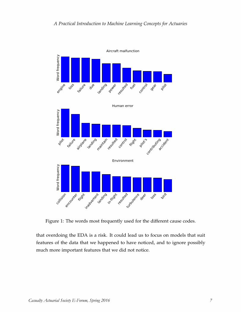
A Practical Introduction to Machine Learning Concepts for Actuaries
engi
ne loss
failu
re
due
land
ing
power
resu
lted
fuel
cont
rol
gear
pilo
t
Word
fre
quency
Aircraft malfunction
pilo
t
failu
reai
rpla
nela
ndin
gm
aint
ain
resu
lted
cont
rol
fligh
t
pilo
t sco
ntrib
utin
gac
cide
nt
Word
fre
quency
Human error
colli
sion
enco
unte
rfli
ght
inad
verten
tla
ndin
gin
-flig
htre
sulte
dtu
rbul
ence
deer
loss
bird
Word
fre
quency
Environment
Figure 1: The words most frequently used for the different cause codes.
that overdoing the EDA is a risk. It could lead us to focus on models that suit features of the data that we happened to have noticed, and to ignore possibly much more important features that we did not notice.
Casualty Actuarial Society E-Forum, Spring 2016 7
A Practical Introduction to Machine Learning Concepts for Actuaries
3.3 Feature Engineering
When an Actuary creates a predictive model (for claims frequency, say), he will have to decide on risk factors to be included in the modelling process. These might include the age of the policyholder and the geo-location. The data which is fed into the model will typically be one record per customer per year, with each record containing all the risk factors and whether or not the customer reported any claims.
In Machine Learning parlance, each record is called an example, and the risk factors are called features. We use features to represent the example, and we seek to find a relationship (or function) between the features and whether or not the customer filed any c laims. Sometimes, the features we really need are not included in the raw data. For example, in car insurance power-weight ratio may not be in the raw data. Within health insurance, height-weight ratio may not be in the raw data. If the model we are using is exceedingly flexible or powerful, it might be able to find these relationships even without us calculating t hem. However, for simple models such as generalised linear models, we need to calculate such features ourselves. We need to use our domain expertise and understanding of the real world to propose and calculate features. This is called feature engineering. Likewise, enriching internally gathered data with external data sources is feature engineering.
Finding and exploring new features is critical to creating good or improved models. Many hours might be spent on fine tuning a model to gain some small improvement, whereas finding a new and useful feature would provide significant improvement.
For our task in this paper, given the type of models that we fit, w e n eed to manually find a way to represent t he n arratives by f eatures s o t hat we c an fit models. The simplest way to do this is to count the occurrences of selected specific words in each narrative, and we discuss this is further detail next.
Casualty Actuarial Society E-Forum, Spring 2016 8
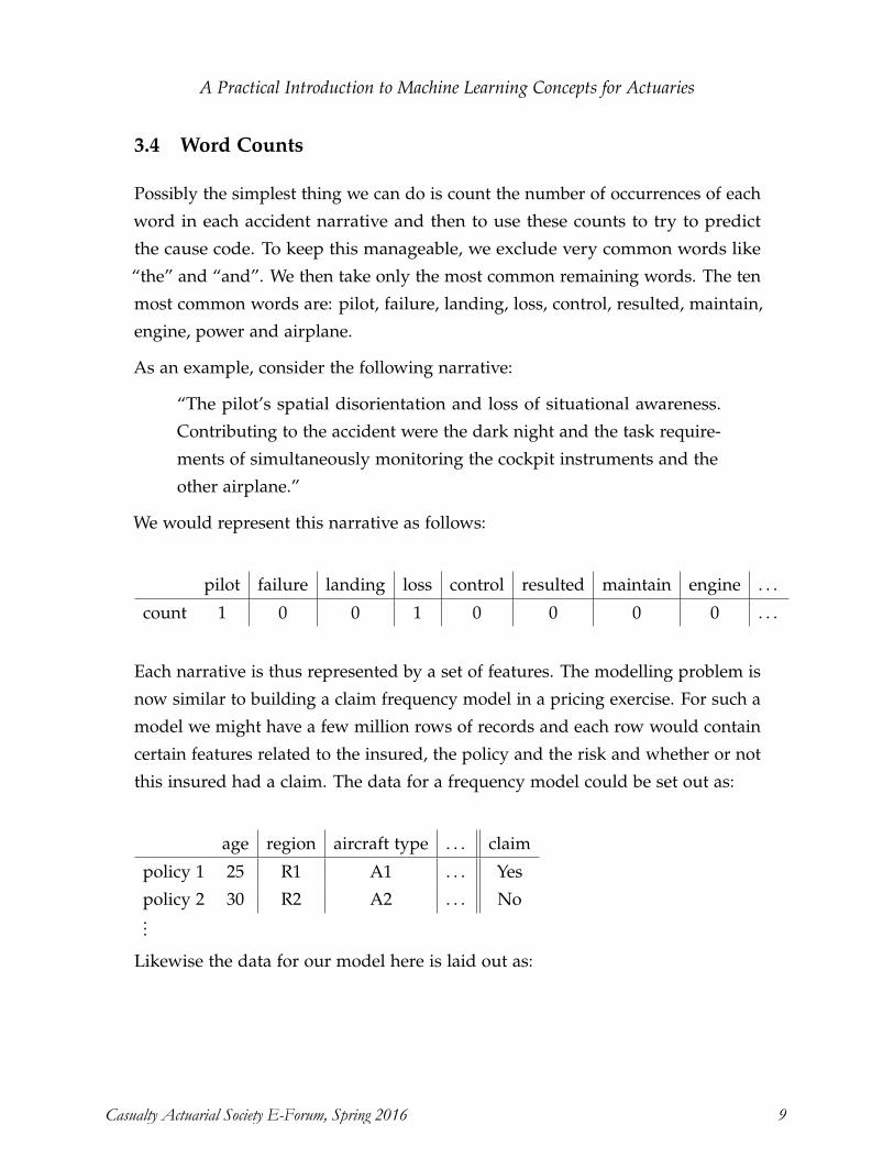
A Practical Introduction to Machine Learning Concepts for Actuaries
3.4 Word Counts
Possibly the simplest thing we can do is count the number of occurrences of each
word in each accident narrative and then to use these counts to try to predict
the cause code. To keep this manageable, we exclude very common words like
“the” and “and”. We then take only the most common remaining words. The ten
most common words are: pilot, failure, landing, loss, control, resulted, maintain,
engine, power and airplane.
As an example, consider the following narrative:
“The pilot’s spatial disorientation and loss of situational awareness.
Contributing to the accident were the dark night and the task require-
ments of simultaneously monitoring the cockpit instruments and the
other airplane.”
We would represent this narrative as follows:
pilot failure landing loss control resulted maintain engine . . .
count 1 0 0 1 0 0 0 0 . . .
Each narrative is thus represented by a set of features. The modelling problem is
now similar to building a claim frequency model in a pricing exercise. For such a
model we might have a few million rows of records and each row would contain
certain features related to the insured, the policy and the risk and whether or not
this insured had a claim. The data for a frequency model could be set out as:
age region aircraft type . . . claim
policy 1 25 R1 A1 . . . Yes
policy 2 30 R2 A2 . . . No...
Likewise the data for our model here is laid out as:
Casualty Actuarial Society E-Forum, Spring 2016 9
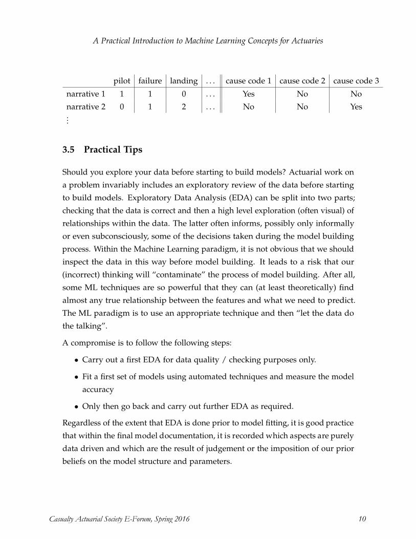
A Practical Introduction to Machine Learning Concepts for Actuaries
pilot failure landing . . . cause code 1 cause code 2 cause code 3
narrative 1 1 1 0 . . . Yes No No
narrative 2 0 1 2 . . . No No Yes...
3.5 Practical Tips
Should you explore your data before starting to build models? Actuarial work on
a problem invariably includes an exploratory review of the data before starting
to build models. Exploratory Data Analysis (EDA) can be split into two parts;
checking that the data is correct and then a high level exploration (often visual) of
relationships within the data. The latter often informs, possibly only informally
or even subconsciously, some of the decisions taken during the model building
process. Within the Machine Learning paradigm, it is not obvious that we should
inspect the data in this way before model building. It leads to a risk that our
(incorrect) thinking will “contaminate” the process of model building. After all,
some ML techniques are so powerful that they can (at least theoretically) find
almost any true relationship between the features and what we need to predict.
The ML paradigm is to use an appropriate technique and then “let the data do
the talking”.
A compromise is to follow the following steps:
• Carry out a first EDA for data quality / checking purposes only.
• Fit a first set of models using automated techniques and measure the model
accuracy
• Only then go back and carry out further EDA as required.
Regardless of the extent that EDA is done prior to model fitting, it is good practice that within the final model documentation, it is recorded which aspects are purely data driven and which are the result of judgement or the imposition of our prior beliefs on the model structure and parameters.
Casualty Actuarial Society E-Forum, Spring 2016 10
A Practical Introduction to Machine Learning Concepts for Actuaries
4. LOGISTIC REGRESSION
Now that we have engineered a set of features that can be used to represent
each example, we can move onto our first model. We will start with a logistic
regression. Logistic regression is part of the generalised linear model family and
will have been used in practice by many Actuaries in building frequency models
for insurance claims frequency.
As mentioned previously, one difference between our task here and other tasks, is
that each narrative can have more than one label. For example, when building
claims frequency models, each policy can have 0 or 1 or 2 . . . claims. When
described like this (rather than as a continuous frequency per unit exposure),
such a problem is called “multi-class”. That is to say, each policy can belong to
the class of insureds that claim once, or the class that claims twice and so on.
In this example each policy can belong to one and only one class. However, in
our case each policy can belong to more than one class. Such a problem is called
“multi-label”. There are specific ways of dealing well with a multi-label problem,
but because they are not broadly relevant to Actuarial work we do not use them
here. Rather, we simply focus on predicting whether or not a narrative has been
coded as cause code 01-Aircraft.
4.1 Results
The result of application of Logistic Regression is a scoring algorithm which can be
applied to existing examples or to new examples. The score to be assigned to the
claims narrative is based on the features that we fed into the Logistic Regression.
In our case, these are word counts. Once a logistic regression model has been
fitted, in order to decide which cause code to assign a given claims narrative, we
carry out the following steps:
• Find the score for each word in the claims narrative.
• Sum all the word scores to give a score for the sentence.
• Convert the score into a “probability” that the claims narrative should be
Casualty Actuarial Society E-Forum, Spring 2016 11
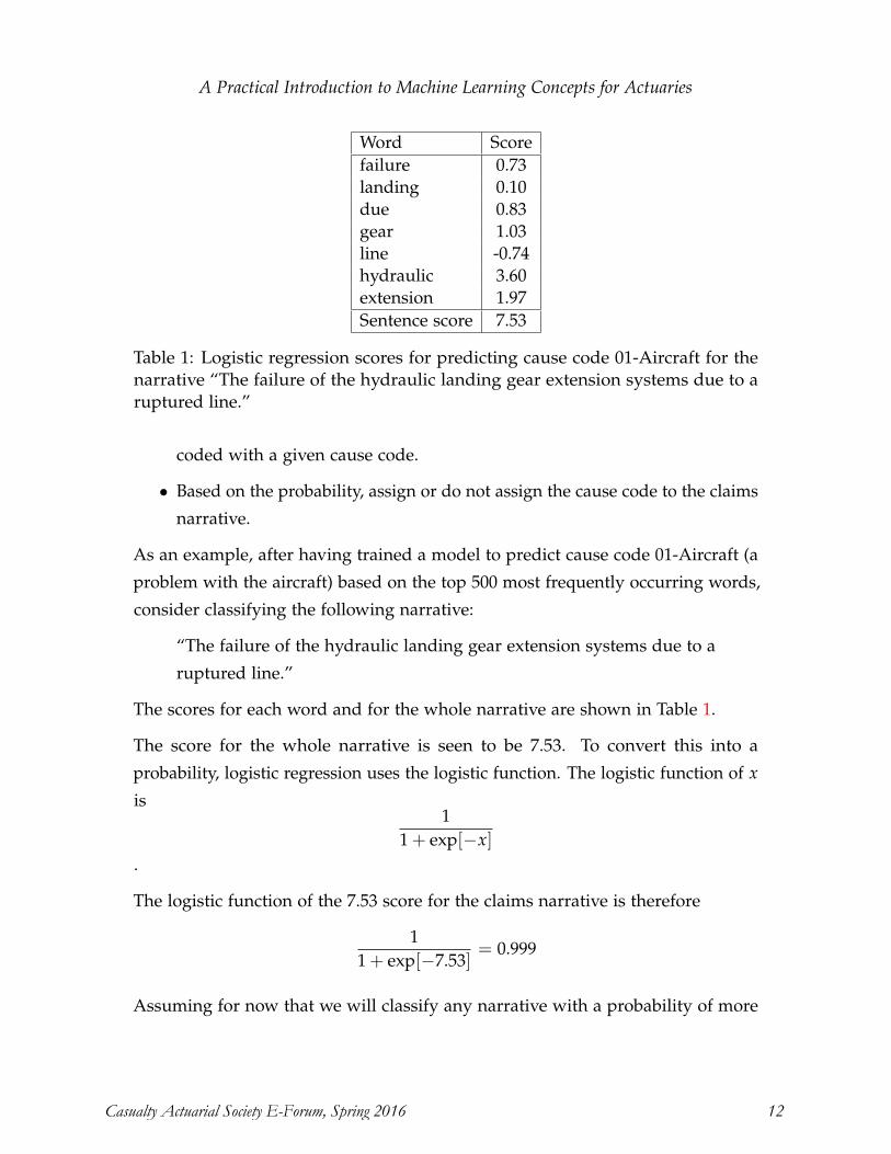
A Practical Introduction to Machine Learning Concepts for Actuaries
Word Scorefailure 0.73landing 0.10due 0.83gear 1.03line -0.74hydraulic 3.60extension 1.97Sentence score 7.53
Table 1: Logistic regression scores for predicting cause code 01-Aircraft for thenarrative “The failure of the hydraulic landing gear extension systems due to aruptured line.”
coded with a given cause code.
• Based on the probability, assign or do not assign the cause code to the claims
narrative.
As an example, after having trained a model to predict cause code 01-Aircraft (a
problem with the aircraft) based on the top 500 most frequently occurring words,
consider classifying the following narrative:
“The failure of the hydraulic landing gear extension systems due to a
ruptured line.”
The scores for each word and for the whole narrative are shown in Table 1.
The score for the whole narrative is seen to be 7.53. To convert this into a
probability, logistic regression uses the logistic function. The logistic function of x
is1
1 + exp[−x].
The logistic function of the 7.53 score for the claims narrative is therefore
11 + exp[−7.53]
= 0.999
Assuming for now that we will classify any narrative with a probability of more
Casualty Actuarial Society E-Forum, Spring 2016 12

A Practical Introduction to Machine Learning Concepts for Actuaries
than 0.50 as cause code 01, we do indeed classify this narrative as a problem with the aircraft.
4.2 Interpretation
Many ML techniques result in models which are not easily interpretable. By this we mean that, if an interested party were to ask for the exact formula to use to make future predictions, it would be difficult to give the answer in a simple form. For certain applications this can matter a lot. For example, we might predict a medication to be efficacious for one patient and not for another, and, when we were challenged as to which features drive this conclusion and the magnitude of the effect of each feature, we would be unable to give a simple answer. Medical professionals might find it difficult to take decisions based on the output of such a model. In an insurance context, a model which predicts that a customer should have a price increase, but leaves an underwriter unable to understand exactly why this is the case, may be difficult for the underwriter to implement in practice .(We will actually see later that often, with some effort, even the more complex ML models can be interpreted to some extent.)
The predictions given by a logistic regression can be easily understood, and hence, we can gain insight into what words will drive the prediction of a future example. For example, looking at words with the highest absolute score gives us an idea of which words will cause a sentence to be classified one way or the o ther. The ten words with the largest (absolute) scores for predicting cause codes 01, 02 and 03 are shown in Table 2. We would have expected that sentences with words like “turbine”, “oil” and “cylinder” would lead us to predict that a narrative is cause 01-Aircraft, and that is indeed the case.
Words having a high absolute score are not necessarily the most important words for classification of future e xamples. Indeed, the careful reader may have been surprised that the word “pilot” is not present in cause 02-Human Error above. The above words may have high scores, but they may not occur very frequently. The scores for the ten most frequently occurring words are shown in Table 6. We see that indeed the word “pilot” does have quite a high score in the model predicting
Casualty Actuarial Society E-Forum, Spring 2016 13
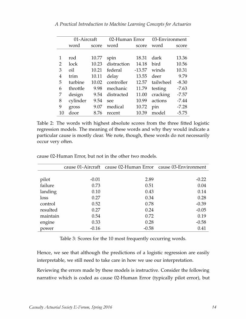
A Practical Introduction to Machine Learning Concepts for Actuaries
01-Aircraft 02-Human Error 03-Environmentword score word score word score
1 rod 10.77 spin 18.31 dark 13.362 lock 10.23 distraction 14.18 bird 10.563 oil 10.21 federal -13.57 winds 10.314 trim 10.11 delay 13.55 deer 9.795 turbine 10.02 controller 12.57 tailwheel -8.306 throttle 9.98 mechanic 11.79 testing -7.637 design 9.54 distracted 11.00 cracking -7.578 cylinder 9.54 see 10.99 actions -7.449 gross 9.07 medical 10.72 pin -7.2810 door 8.76 recent 10.39 model -5.75
Table 2: The words with highest absolute scores from the three fitted logisticregression models. The meaning of these words and why they would indicate aparticular cause is mostly clear. We note, though, these words do not necessarilyoccur very often.
cause 02-Human Error, but not in the other two models.
cause 01-Aircraft cause 02-Human Error cause 03-Environment
pilot -0.01 2.89 -0.22failure 0.73 0.51 0.04landing 0.10 0.43 0.14loss 0.27 0.34 0.28control 0.52 0.78 -0.39resulted 0.27 0.24 -0.05maintain 0.54 0.72 0.19engine 0.33 0.28 -0.58power -0.16 -0.58 0.41
Table 3: Scores for the 10 most frequently occurring words.
Hence, we see that although the predictions of a logistic regression are easily interpretable, we still need to take care in how we use our interpretation.
Reviewing the errors made by these models is instructive. Consider the following narrative which is coded as cause 02-Human Error (typically pilot error), but
Casualty Actuarial Society E-Forum, Spring 2016 14
A Practical Introduction to Machine Learning Concepts for Actuaries
which was not predicted as such by the model:
“The pilot’s failure to maintain airspeed and aircraft control, resulting
in an aerodynamic stall.”
This is obviously pilot error as it contains the phrase “pilot’s failure”, yet the logistic regression fails to classify it correctly. The reason for this misclassification is that the word “failure” is more often associated with the failure of a part of the aircraft than it is with pilot failure. Were we to represent the document not just by word counts but by counts of phrases of two words (bi-grams) such as “pilot’s failure”, we should expect to see some improvement in accuracy. The process of considering which extra features to calculate and to add to the model input is called “feature engineering”.
4.3 How It Works
Each time we use a model, we should try to understand how it works. This is especially important for certain Machine Learning models where it is not obvious at first sight what the model is d oing. Logistic regression is not what we might call a Machine Learning model. It has a long history in traditional statistics and is part of the generalised linear model family. Nonetheless, we provide some brief comments below.
Consider a logistic regression model used to find the true p robability, p , of an insured customer having an accident. In order to create a useful model, we relate p for each customer to the features of that customer. The features might be things like age, vehicle type and so on. If we are using n features in our model, then for customer j we will refer to his features as:
x(1j), x(2
j), . . . , x(nj).
We need to convert these features into our estimate of p(j), the true risk for customer j. We will do this by finding a coefficient for each feature,
β1, β2, . . . , β j.
Casualty Actuarial Society E-Forum, Spring 2016 15
A Practical Introduction to Machine Learning Concepts for Actuaries
These coefficients are the scores we referred to in subsection 4.1 above.
Finding these coefficients is hard (see Section 5) , but once it is done, the process
for finding p is exactly the same as our discussion in subsection 4.1. We first find
η(j) = β1x(j)1 + β2x(j)
2 + · · ·+ β jx(j)n .
Then we say that
p(j) = logistic[η(j)].
In our example in subsection 4.1, η worked out to 7.53 and then we had
logistic(7.53) =1
1 + exp[−7.53]= 0.999.
Using the logistic function ensures that output of the model is between 0 and 1.
The main work of this model is done by finding
η(j) = β1x(j)1 + β2x(j)
2 + · · ·+ β jx(j)n .
If η(j) is large, the estimated p(j) will be large, and, if used for classification, the
example is classified as 1 or “Yes”. If η(j) is low, the estimated p(j) will be small,
and, if used for classification, the example is classified as 0 or “No”. η(j) depends
on the β’s in a linear way. Hence, the model is just a simple linear model at
heart and really only gives us access to simple ways to find relationships between
features of the examples and things we wish to predict about the examples. In our
task this might be not such a limitation since the value for most of the features is
only 0 or 1 most of the time and, therefore, the relationship for any one feature can
be expressed in a linear way. However, more generally, it should not be surprising
if models that can express non-linear relationships can do bettter than “vanilla”
logistic regression.
4.4 Practical Tips
• Reproducibility. Logistic regression is not an equation that can be solved
with a simple formula. When using some software, a very slightly different
Casualty Actuarial Society E-Forum, Spring 2016 16
A Practical Introduction to Machine Learning Concepts for Actuaries
answer may result each time the logistic regression is run, even when using
the same data. It is often a good idea to specifically set the random seed
used by the software to ensure reproducibility.
• Check the default settings of your software. Regularisation, an idea we will
discuss in a following section, is such an obvious thing to do, that some
software now do it by default. In particular sci-kit learn, the Python module
used for this project will carry out some form of regularisation by default
and we needed to ensure that it was “turned off”, in order to produce the
results in this section.
4.5 Summary and Next Steps
So far we have a seen a simple logistic regression model. There are, however,
many unanswered questions:
• How good is our model?
• Even if we know our model is good for existing examples, how do we know
if our model is any good for future examples?
• We used the 500 most frequently occurring words? We could equally as well
only have used the top 10 occurring words or the top 2000. How do we
know which is best?
• We saw that some words occur very frequently and some occur far less
frequently. This means that the average word count will be much higher
for some words than for others. Does this matter? Can we do anything to
check?
• Can we add other features to our model which will help improve predictive
power?
To answer these questions, we will need to discuss various key areas of Machine
Learning practice:
• Model evaluation measures (Section 6)
Casualty Actuarial Society E-Forum, Spring 2016 17
A Practical Introduction to Machine Learning Concepts for Actuaries
• Generalisation and model validation (Section 7)
• Feature scaling (Section 8)
• Regularisation (Section 9)
• Feature engineering (Section 10)
Before discussing model evaluation, we consider another critical aspect of Machine Learning thought, the loss function.
5. LOSS FUNCTIONS
The idea of telling the machine exactly what matters and then letting the machine automatically find t he b est m odel w ithin a c lass o f m odels i s f undamental to Machine Learning thought. We tell the machine “what matters” by defining a “loss function” which is high when the fitted m odel i s “ bad” i n s ome way and “low” when the fitted model is g ood. We then simply have a minimisation problem: we need to minimise the loss function. (The meaning of loss function in this paper should not be confused with its use in actuarial work where it is sometimes taken to mean the distribution function for claims severity.)
There is often a duality between looking at predictive modelling as a task in maximising some kind of statistical likelihood or probability on the one hand, or treating the task as loss function minimisation on the other hand. In this section we demonstrate this duality for the logistic regression model discussed in Section 4. In other words, solving the problem of logistic regression from a maximum likelihood perspective gives exactly the same result as treating the problem as an exercise in minimising the sum of errors where the value of each error is defined by a certain loss f unction. Why bother with loss functions when maximum likelihood gives the same answer? It turns out that they provide flexibility in designing powerful ranges of m odels. This flexibility is not as easily available under the probabilistic approach.
Casualty Actuarial Society E-Forum, Spring 2016 18
A Practical Introduction to Machine Learning Concepts for Actuaries
5.1 The Maximum Likelihood Approach
Let us start with the maximum likelihood approach to logistic regression. We will
show how this works from first principles. (Reading this section is not critical for
the flow of the paper, but will give useful insight into the link between traditional
approaches and more general ML techniques.)
We step away from our text prediction task for a moment and consider a model to
predict whether or not a customer will make an insurance claim. A traditional
view of logistic regression is as follows: for any customer we are looking at, let
“Claim” be a random variable which takes value 1 if that customer ends up making
a claim and 0 if not. Let p be the probability that the customer will make a claim,
i.e., Pr[Claim = 1] = p. In other words, “Claim” follows a Bernoulli distribution
with probability p. If we had to guess in advance whether a customer would make
a claim and we knew the value of p, we would guess “yes” if p > 0.5. However,
we don’t know p for new customers. In fact, we don’t even know the value of
p for existing customers, we only know whether or not they made a claim. It is
possible that p, the true risk of a customer making a claim, is 0.99, yet they were
fortunate and did not have an incident in the past year.
We saw in subsection 4.3 that solving a logistic regression requires us to find the
best set of βs where:
η(j) = β1x(j)1 + β2x(j)
2 + · · ·+ β jx(j)n (1)
and
p(j) = logistic[η(j)]. (2)
The traditional statistical way is to approach this from a probabilistic perspective. We certainly know whether each existing customer has claimed or not. Let a(j) = 1 if customer j claimed and 0 otherwise. Assume for now that we know p(j) for customer j. If they did indeed claim, then the likelihood of this is p(j). Since in this case, a(j) = 1, we can express this as:
(p(j))a(j) = (p(j))1 = p(j).
Casualty Actuarial Society E-Forum, Spring 2016 19
A Practical Introduction to Machine Learning Concepts for Actuaries
Likewise if they did not claim, then the likelihood of this is 1 − p(j). Since in this
case, a(j) = 0, we can express this as:
(1 − p(j))(1−a(j)) = (1 − p(j))(1−0) = (1 − p(j))1 = 1 − p(j).
So, regardless of whether the customer claimed or not, we can write this expression
more generally as:
(p(j))a(j) × (1 − p(j))(1−a(j))
because, if the customer did claim, then the first part of the expression works out
correctly and the second part is just 1 and vice versa.
Our aim is then to find the set of p(j) such that the likelihood is maximised across
all customers. Assuming that each customers’ claims experience is independent,
the likelihood for all our data is:
L(β) =m
∏j=1
(p(j))a(j) × (1 − p(j))(1−a(j)).
Note that we cannot manipulate the p(j) directly since we have decided in advance
(through equations 1 and 2) that each p(j) is defined by the features of that
customer and by the βs. Since we assume that the features are fixed, all we can
do to maximise the likelihood is to find the set of βs that achieves this. That is
why we write the likelihood as a function of β, i.e., we write L(β) and not L(p).
As usual in this type of approach, we take logs to simplify things. We refer to the
log of the likelihood as log(L(β)) = l(β) and we have
l(β) = log
(m
∏j=1
(p(j))a(j) × (1 − p(j))(1−a(j))
)
=m
∑j=1
a(j) log p(j) + (1 − a(j)) log(1 − p(j))
Hence the problem of finding the maximum likelihood solution to logistic regres-
sion is to find the βs that maximise the above expression i.e.
β̂ = argmaxβ
m
∑j=1
[a(j) log p(j) + (1 − a(j)) log(1 − p(j))
](3)
Casualty Actuarial Society E-Forum, Spring 2016 20
A Practical Introduction to Machine Learning Concepts for Actuaries
where
p(j) = logistic
[n
∑i=1
βix(j)i
]
5.2 The Loss Function Approach
Imagine that you have two possible solutions to a problem. How do you choose one solution over the other? You need a way to evaluate each solution. One way to evaluate solutions is to calculate the predictions and to charge some kind of loss for each incorrect prediction. We sum these charges and call the sum the ”loss”. We can do this for every solution which is provided to us and we then simply choose the solution with the smallest loss.
If we are predicting something which can be classified a s o ne o f a number of categories, we could simply say that the contribution to the loss is 1 if the prediction is wrong and 0 if the prediction is correct. The overall loss will then simply be the total number of errors made by the predictive algorithm. For obvious reasons this is known as the zero-one loss.
Consider the zero-one loss function further. If the result of a logistic regression for a customer is that p = 0.75, then since p > 0.5 we classify that customer as Claim = 1. If in fact that customer does not claim, then the loss is 1. The same loss would occur if p = 0.51 or p = 0.99. However, given that the customer did not claim, we might instinctively feel that a predictive algorithm which found p = 0.51 is better than one which finds p = 0 .99. There is a loss function, called “cross entropy”, which deals well with this issue and also has theoretically useful properties. If a is the actual class (which is either 0 or 1) and p is the result of our classifier, then cross entropy is defined as follows:
CE(a, p) = −a log p − (1 − a) log(1 − p)
To see how this works, consider the case when a = 0 (i.e., the customer did not claim). Then we have:
CE(a = 0, p) = −0 log p − (1 − 0) log(1 − p) = − log(1 − p).
Casualty Actuarial Society E-Forum, Spring 2016 21
A Practical Introduction to Machine Learning Concepts for Actuaries
If p = 0.99 then the cross entropy is:
CE(a = 0, p = 0.99) = − log(1 − 0.99) = +4.6.
and if p = 0.51 then the cross entropy is:
CE(a = 0, p = 0.51) = − log(1 − 0.51) = +0.71
Clearly the loss gets smaller as p gets closer to zero.
If we use cross-entropy as our measure of loss, then the best βs are the ones which
minimize the loss across all customers, hence we need to find:
β̂ = argminβ
m
∑j=1
[−a(j) log p(j) − (1 − a(j)) log(1 − p(j))
]= argmax
β
m
∑j=1
[a(j) log p(j) + (1 − a(j)) log(1 − p(j))
](4)
We can now see that the equation for finding the βs using Maximum Likelihood
(equation 3) is exactly the same as that for finding the βs using the cross-entropy
loss function (equation 4). Many Actuaries may be used to thinking of finding the
best solution to a model as a maximum likelihood problem. Understanding that
this is infact identical to minimising a loss function provides a bridge to many
Machine Learning techniques.
We are now ready to move on to the questions raised at the end of Section 4, and
we start with a discussion of how best to evaluate model performance.
6. MODEL EVALUATION
Consider this question:
How good, objectively, is your model?
A comprehensive answer for a claims severity model might be:
90% of the time my model predicts claims severity within 50% of the actual outcome and the remaining 10% of the time it is never more than 80% out.
Casualty Actuarial Society E-Forum, Spring 2016 22
A Practical Introduction to Machine Learning Concepts for Actuaries
Practitioners involved in building insurance pricing models often “know” that the generalised linear model that they fitted is the “best” in some way because it was arrived at by a process of stepwise selection, that AIC / BIC (Akaike /Bayes Information Criterion) was minimised, or some other statistical process was followed in fitting the m odel. However, these statements are not really helpful. The best model from amongst many bad models is not necessarily a good model. Nor are these definitions of best particularly e nlightening. Therefore, thinking through what measure should be used to evaluate model performance and to compare this measure between alternative models is a useful process. In this way we can objectively measure model performance, find the best model and know whether or not it is fit for purpose.
In practice, there are various reasons that we might decide not to use the best performing model. For example, it may take a prohibitively long time to find the correct parameters for the model. It might be that even if we know the parameters of a model, when we get a new claims narrative to classify, it takes a long time to run it through the model. There is also the issue of model transparency and interpretability (see the discussion in subsection 4.2).
Despite the above, measuring model performance plays a key part in deciding which model to use. Even if the model with the best performance is not used, it can act as a benchmark so that we know how far short the models actually implemented are of best performance.
This section motivates and describes some possible model evaluation measures for our task. We then choose one measure which we use throughout the rest of our work.
6.1 Classification or Regression
The measure we use depends first and foremost on whether the thing that we wish to predict is categorical or continuous. In Machine Learning (and statistical) parlance, models which predict a continuous variable are called regression models and models which predict categorical variables are called classification models.
Casualty Actuarial Society E-Forum, Spring 2016 23
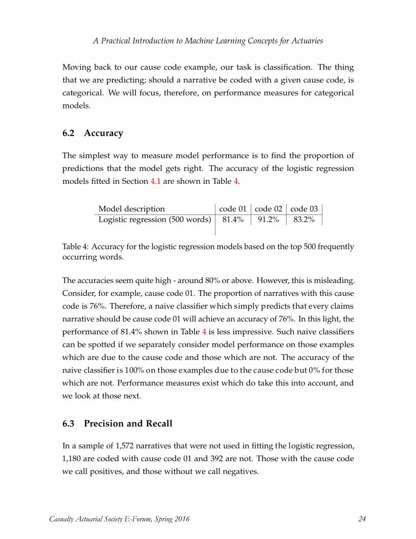
A Practical Introduction to Machine Learning Concepts for Actuaries
Moving back to our cause code example, our task is classification. The thing
that we are predicting; should a narrative be coded with a given cause code, is
categorical. We will focus, therefore, on performance measures for categorical
models.
6.2 Accuracy
The simplest way to measure model performance is to find the proportion of
predictions that the model gets right. The accuracy of the logistic regression
models fitted in Section 4.1 are shown in Table 4.
Model description code 01 code 02 code 03Logistic regression (500 words) 81.4% 91.2% 83.2%
Table 4: Accuracy for the logistic regression models based on the top 500 frequently occurring words.
The accuracies seem quite high - around 80% or above. However, this is misleading. Consider, for example, cause code 01. The proportion of narratives with this cause code is 76%. Therefore, a naive classifier which simply predicts that every claims narrative should be cause code 01 will achieve an accuracy of 76%. In this light, the performance of 81.4% shown in Table 4 is less impressive. Such naive classifiers can be spotted if we separately consider model performance on those examples which are due to the cause code and those which are not. The accuracy of the naive classifier is 100% on those examples due to the cause code but 0% for those which are not. Performance measures exist which do take this into account, and we look at those next.
6.3 Precision and Recall
In a sample of 1,572 narratives that were not used in fitting the logistic regression, 1,180 are coded with cause code 01 and 392 are not. Those with the cause code we call positives, and those without we call negatives.
Casualty Actuarial Society E-Forum, Spring 2016 24
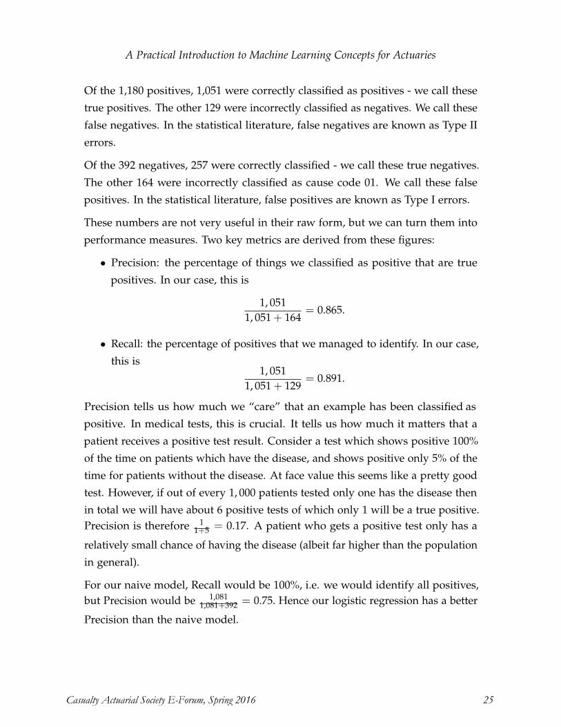
A Practical Introduction to Machine Learning Concepts for Actuaries
Of the 1,180 positives, 1,051 were correctly classified as positives - we call these
true positives. The other 129 were incorrectly classified as negatives. We call these
false negatives. In the statistical literature, false negatives are known as Type II
errors.
Of the 392 negatives, 257 were correctly classified - we call these true negatives.
The other 164 were incorrectly classified as cause code 01. We call these false
positives. In the statistical literature, false positives are known as Type I errors.
These numbers are not very useful in their raw form, but we can turn them into
performance measures. Two key metrics are derived from these figures:
• Precision: the percentage of things we classified as positive that are true
positives. In our case, this is
1, 0511, 051 + 164
= 0.865.
• Recall: the percentage of positives that we managed to identify. In our case,
this is1, 051
1, 051 + 129= 0.891.
Precision tells us how much we “care” that an example has been classified as positive. In medical tests, this is crucial. It tells us how much it matters that a patient receives a positive test result. Consider a test which shows positive 100%
of the time on patients which have the disease, and shows positive only 5% of the time for patients without the disease. At face value this seems like a pretty good test. However, if out of every 1, 000 patients tested only one has the disease then in total we will have about 6 positive tests of which only 1 will be a true positive. Precision is therefore 1
1+5 = 0.17. A patient who gets a positive test only has a
relatively small chance of having the disease (albeit far higher than the population in general).
For our naive model, Recall would be 100%, i.e. we would identify all positives, but Precision would be 1,081
1,081+392 = 0.75. Hence our logistic regression has a better
Precision than the naive model.
Casualty Actuarial Society E-Forum, Spring 2016 25
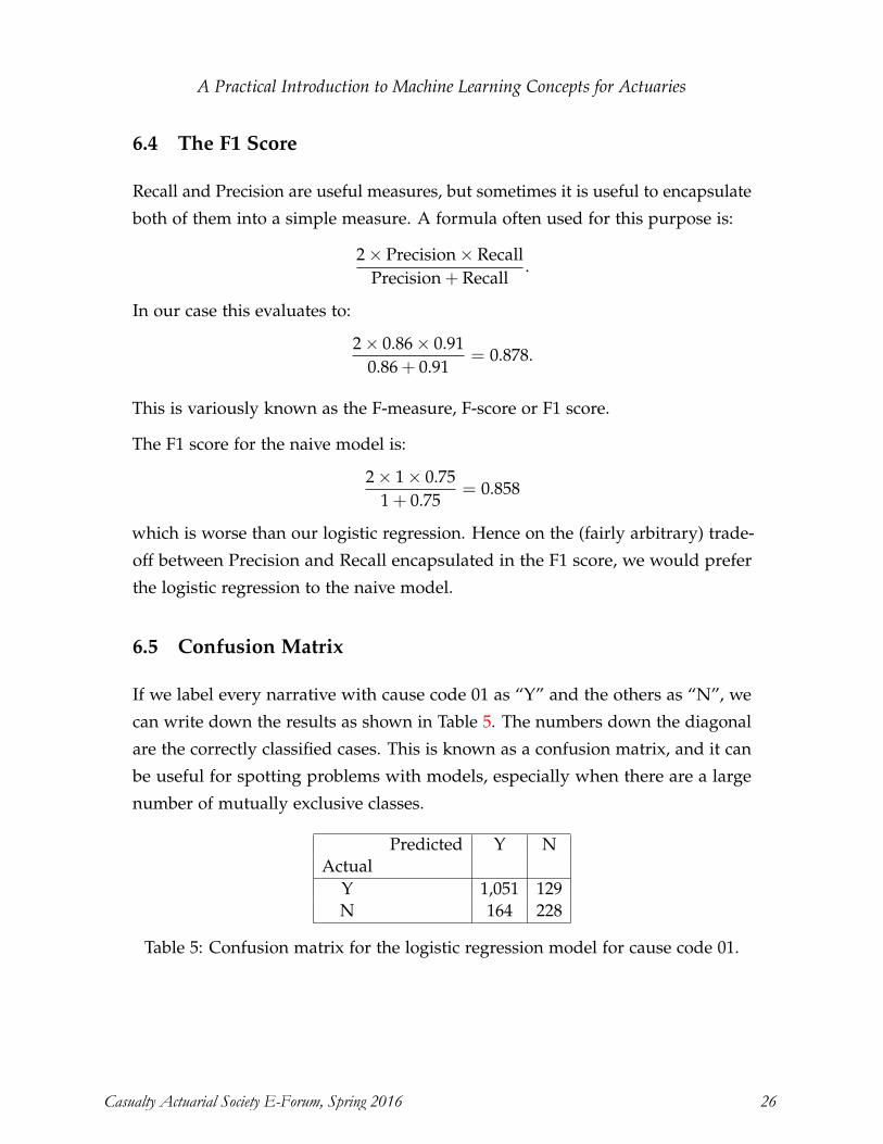
A Practical Introduction to Machine Learning Concepts for Actuaries
6.4 The F1 Score
Recall and Precision are useful measures, but sometimes it is useful to encapsulate
both of them into a simple measure. A formula often used for this purpose is:
2 × Precision × RecallPrecision + Recall
.
In our case this evaluates to:
2 × 0.86 × 0.910.86 + 0.91
= 0.878.
This is variously known as the F-measure, F-score or F1 score.
The F1 score for the naive model is:
2 × 1 × 0.751 + 0.75
= 0.858
which is worse than our logistic regression. Hence on the (fairly arbitrary) trade-
off between Precision and Recall encapsulated in the F1 score, we would prefer
the logistic regression to the naive model.
6.5 Confusion Matrix
If we label every narrative with cause code 01 as “Y” and the others as “N”, we
can write down the results as shown in Table 5. The numbers down the diagonal
are the correctly classified cases. This is known as a confusion matrix, and it can
be useful for spotting problems with models, especially when there are a large
number of mutually exclusive classes.
Predicted Y NActual
Y 1,051 129N 164 228
Table 5: Confusion matrix for the logistic regression model for cause code 01.
Casualty Actuarial Society E-Forum, Spring 2016 26
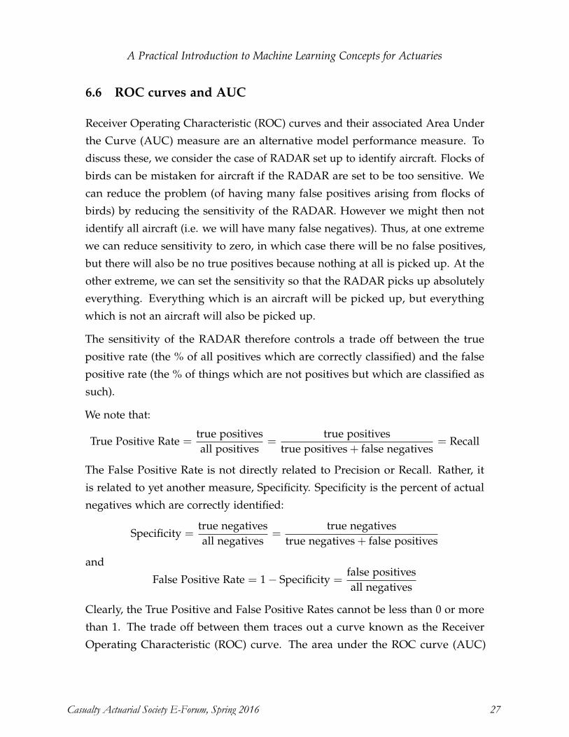
A Practical Introduction to Machine Learning Concepts for Actuaries
6.6 ROC curves and AUC
Receiver Operating Characteristic (ROC) curves and their associated Area Under
the Curve (AUC) measure are an alternative model performance measure. To
discuss these, we consider the case of RADAR set up to identify aircraft. Flocks of
birds can be mistaken for aircraft if the RADAR are set to be too sensitive. We
can reduce the problem (of having many false positives arising from flocks of
birds) by reducing the sensitivity of the RADAR. However we might then not
identify all aircraft (i.e. we will have many false negatives). Thus, at one extreme
we can reduce sensitivity to zero, in which case there will be no false positives,
but there will also be no true positives because nothing at all is picked up. At the
other extreme, we can set the sensitivity so that the RADAR picks up absolutely
everything. Everything which is an aircraft will be picked up, but everything
which is not an aircraft will also be picked up.
The sensitivity of the RADAR therefore controls a trade off between the true
positive rate (the % of all positives which are correctly classified) and the false
positive rate (the % of things which are not positives but which are classified as
such).
We note that:
True Positive Rate =true positivesall positives
=true positives
true positives + false negatives= Recall
The False Positive Rate is not directly related to Precision or Recall. Rather, it
is related to yet another measure, Specificity. Specificity is the percent of actual
negatives which are correctly identified:
Specificity =true negativesall negatives
=true negatives
true negatives + false positives
and
False Positive Rate = 1 − Specificity =false positivesall negatives
Clearly, the True Positive and False Positive Rates cannot be less than 0 or more than 1. The trade off between them traces out a curve known as the Receiver Operating Characteristic (ROC) curve. The area under the ROC curve (AUC)
Casualty Actuarial Society E-Forum, Spring 2016 27
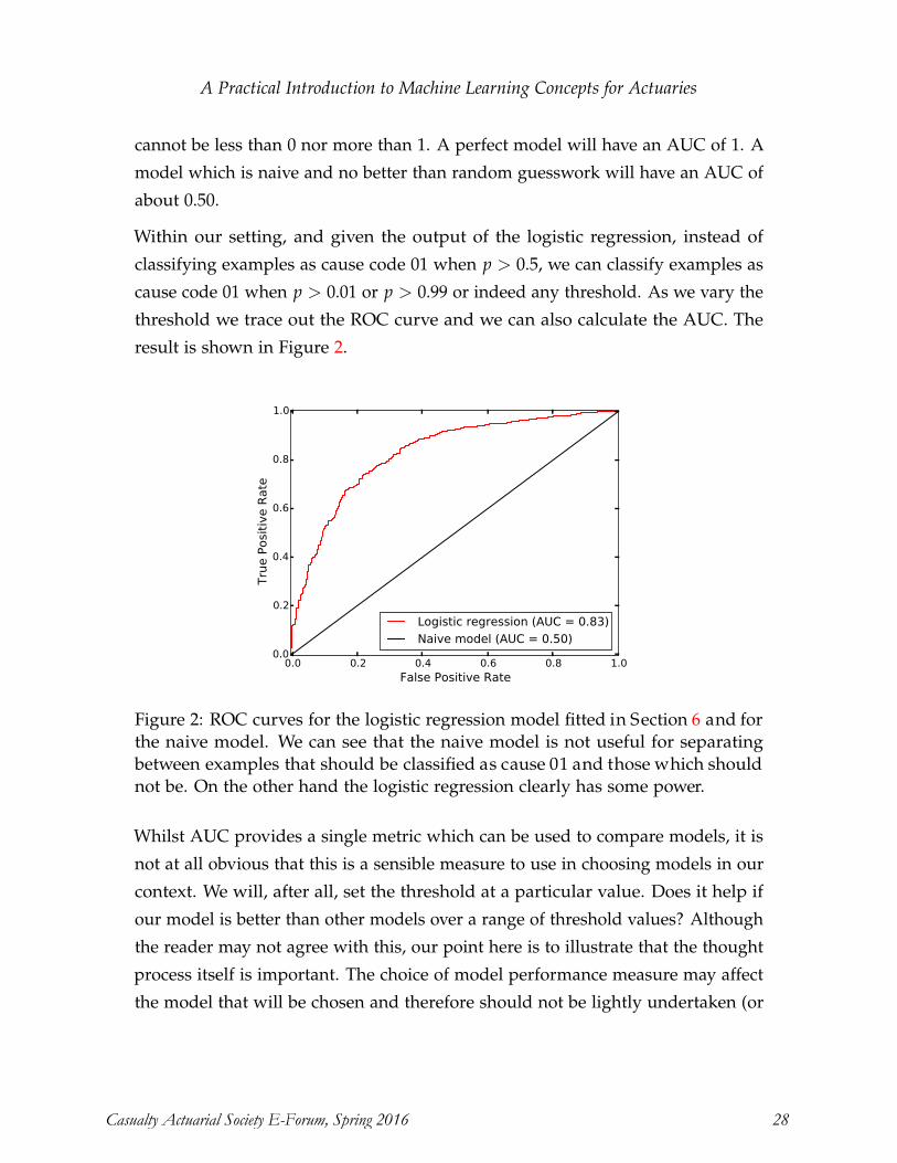
A Practical Introduction to Machine Learning Concepts for Actuaries
cannot be less than 0 nor more than 1. A perfect model will have an AUC of 1. A
model which is naive and no better than random guesswork will have an AUC of
about 0.50.
Within our setting, and given the output of the logistic regression, instead of
classifying examples as cause code 01 when p > 0.5, we can classify examples as
cause code 01 when p > 0.01 or p > 0.99 or indeed any threshold. As we vary the
threshold we trace out the ROC curve and we can also calculate the AUC. The
result is shown in Figure 2.
0.0 0.2 0.4 0.6 0.8 1.0False Positive Rate
0.0
0.2
0.4
0.6
0.8
1.0
Tru
e P
osi
tive R
ate
Logistic regression (AUC = 0.83)
Naive model (AUC = 0.50)
Figure 2: ROC curves for the logistic regression model fitted in Section 6 and for the naive model. We can see that the naive model is not useful for separating between examples that should be classified as cause 01 and those which should not be. On the other hand the logistic regression clearly has some power.
Whilst AUC provides a single metric which can be used to compare models, it is not at all obvious that this is a sensible measure to use in choosing models in our context. We will, after all, set the threshold at a particular value. Does it help if our model is better than other models over a range of threshold values? Although the reader may not agree with this, our point here is to illustrate that the thought process itself is important. The choice of model performance measure may affect the model that will be chosen and therefore should not be lightly undertaken (or
Casualty Actuarial Society E-Forum, Spring 2016 28
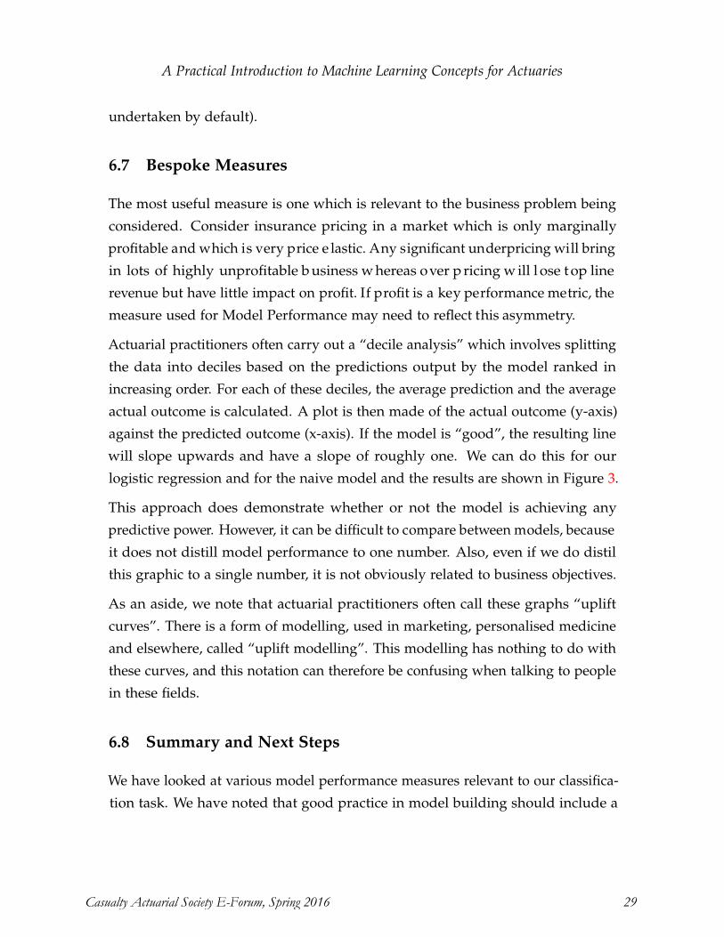
A Practical Introduction to Machine Learning Concepts for Actuaries
undertaken by default).
6.7 Bespoke Measures
The most useful measure is one which is relevant to the business problem being considered. Consider insurance pricing in a market which is only marginally profitable and which is very price e lastic. Any significant underpricing will bring in lots of highly unprofitable b usiness w hereas over p ricing w ill l ose t op line revenue but have little impact on profit. If profit is a key performance metric, the measure used for Model Performance may need to reflect this asymmetry.
Actuarial practitioners often carry out a “decile analysis” which involves splitting the data into deciles based on the predictions output by the model ranked in increasing order. For each of these deciles, the average prediction and the average actual outcome is calculated. A plot is then made of the actual outcome (y-axis) against the predicted outcome (x-axis). If the model is “good”, the resulting line will slope upwards and have a slope of roughly one. We can do this for our logistic regression and for the naive model and the results are shown in Figure 3.
This approach does demonstrate whether or not the model is achieving any predictive power. However, it can be difficult to compare between models, because it does not distill model performance to one number. Also, even if we do distil this graphic to a single number, it is not obviously related to business objectives.
As an aside, we note that actuarial practitioners often call these graphs “uplift curves”. There is a form of modelling, used in marketing, personalised medicine and elsewhere, called “uplift modelling”. This modelling has nothing to do with these curves, and this notation can therefore be confusing when talking to people in these fields.
6.8 Summary and Next Steps
We have looked at various model performance measures relevant to our classifica-
tion task. We have noted that good practice in model building should include a
Casualty Actuarial Society E-Forum, Spring 2016 29
A Practical Introduction to Machine Learning Concepts for Actuaries
0.0 0.2 0.4 0.6 0.8 1.0Predicted: % classified as cause 01
0.0
0.2
0.4
0.6
0.8
1.0
Act
ual: %
cla
ssifie
d a
s ca
use
01
Figure 3: Decile analysis of the the logistic regression model carried out inSection 4. It can be seen that examples that the logistic regression classifies ascause 01 with a high value of p are indeed mostly cause 01. However, the setof examples classified by the logistic regression as not being cause code 01 andwhich have a value of p close to zero are still in fact more than 20% cause code 01.
deliberate and thoughtful choice of performance measure. For our purposes we
will use Accuracy because:
• It is simple.
• It is easy to communicate; i.e., it is meaningful to say that “90% of the time,
our model correctly identifies whether or not a narrative should be coded as
cause 01”.
• For our purposes, the cost of errors are “symmetric”, i.e. it is equally bad to
code a narrative as cause 01 when it is not as it is to miss coding it as cause
01 when it should be.
• There is no specific downstream process which relies on our analysis through
which we could consider more bespoke model performance measures.
We have now addressed the first question raised in subsection 4.5, “How good is our model?” and we move on to the next question, “Even if we know our model
Casualty Actuarial Society E-Forum, Spring 2016 30
A Practical Introduction to Machine Learning Concepts for Actuaries
is a good for existing customers, how do we know if our model is any good at all for future customers?”
7. GENERALISATION ERROR AND MODEL VALIDATION
We have fitted our model based on data on existing n arratives. How do we know if our model will be any good for narratives that we have not yet seen and those that will be written in future? Given the real world context of our own task, we must immediately admit that we cannot have any guarantee at all. This is because the staff in the NTSB who write the narratives and code them could start, from tomorrow, writing the narratives in a totally different style, or coding them in a different way. They may realise that all coding to date was simply wrong and a new approach is needed. In addition, there is a more subtle risk. It could be that across some forms of sentences our model predicts very poorly, but these types of sentences are not frequently in the sample data. Something could change in the future causing these kinds of narratives to become much more common. In this case, model performance will deteriorate in practice even though NTSB staff behaviour has not changed.
Likewise, there are no guarantees in predictive modelling for pricing. Claims-
making behaviour can change across the whole population or within segments. The model can be a poor predictor of frequency for a given segment, and that itself can be the cause of an increase of that type of insured so that overall, the model performs poorly and profitability reduces.
This thought process leads us towards the problems of the model refresh process and optimal timing of model refreshes. This is critical within modelling depart-
ments which may support 100’s of models. We do not consider these issues in this paper inasmuch as they are not specific t o M achine L earning. T hey exist regardless of what type of model is used.
Ignoring for now what might change in the future, how do we know if our model will perform well even if nothing changes? To be precise, we are satisfied assuming that future examples will have the same distribution of features that we
Casualty Actuarial Society E-Forum, Spring 2016 31
A Practical Introduction to Machine Learning Concepts for Actuaries
currently see, and we are also satisfied assuming that the unknown relationship between features and the thing we are trying to predict remains the same. But we still wish to answer the question, how accurate can we expect our model to be for examples we have not yet seen? Generalisation and validation, two ideas which are very much part of the Machine Learning thought process, will help us answer this question, and we now discuss them in some detail.
7.1 The Train-Validation-Test Paradigm
The expected error that our model makes on future, unseen examples is called generalisation error. As we use more features and models of increasing complexity, it is possible that the relationship we find b etween f eatures a nd w hat we are predicting is only due to the vagaries of the data we are looking at and will not apply to future examples.
Traditionally, Actuaries (and Statisticians) have used measures such as AIC or BIC (Akaike / Bayes Information Criterion) to control for this problem. The approach taken in Machine Learning is different and very straightforward. We divide the data that we have available to us now into two datasets. The first dataset is used for fitting t he m odel. T he s econd d ataset i s c alled t he t est s et; i t i s p ut “into a vault” and not used until the end of the model building process. The first dataset is used to fit m odels. We c an fi t as ma ny di fferent mo dels as we like. This may include models from different families (e.g. logistic regression, random forests, or even mixtures of the two). Finally, once we have completed our model building process, we take the test dataset “out of the vault” and calculate the errors of all our different models over the test data. We chose the model with the best generalisation error over the test data. Nowhere within our model building process (except possible in the EDA data quality checks) have we seen this data. Therefore, if our final model has a given generalisation error over the test data, we can reasonably assume that this is reflective of future model performance.
In carrying out our calculations for this paper we followed the same process. On starting our task, we put 20% of our data into the vault. We will only take it out of the vault in Section 11 in order to chose our final model and to estimate
Casualty Actuarial Society E-Forum, Spring 2016 32
A Practical Introduction to Machine Learning Concepts for Actuaries
generalisation error.
We next show how the first d ataset c an b e s plit i nto t raining a nd validation datasets in order to assist model fitting.
7.2 Model Validation, Bias and Variance
Some models are very complex and have various sets of parameters that need fine t uning. At first sight, standard logistic regression is not one of th ese. There is only one set of parameters - the βs, and any statistical software can easily find the best βs. We easily found the best βs when we fitted the model in Section 4. However, we had used only the top 500 most frequently occurring words and we were left with the question of how many words we should use: the top 10? the top 500? the top 5,000? If we use too few words, the model will perform poorly because it does not pick up important relationships between words and cause codes. This source of error is known as bias. If we use too many words, the fitted model will just pick up the vagaries of the sentences we are using and the fitted βs will vary greatly according to which sentences we happen to have access to. This source of error is known as variance. Hence the optimal number of words to use is a parameter which needs to be selected. Only after the parameter for the number of words has been set can a logistic regression be fit. Such parameters are known as hyper-parameters.
To help with this decision, we cannot use the test dataset. It is in the vault and can only be used to choose our final m odel. If we start making modelling decisions based on the test dataset, the model we fit is likely to perform better on the test dataset than on future, unknown examples. Neither can we use the dataset we are using for modelling. If we use that, we will simply find that the larger the number of words we use, the better. This is exactly the overfitting we are looking to avoid.
Instead, we split the remaining data (randomly) into a training set and a validation set. In our case, we put 80% into the training set and 20% into the validation set.
Next we fit many models on the training dataset, and we measure the accuracy on both the training dataset and the validation dataset for each model. The result
Casualty Actuarial Society E-Forum, Spring 2016 33
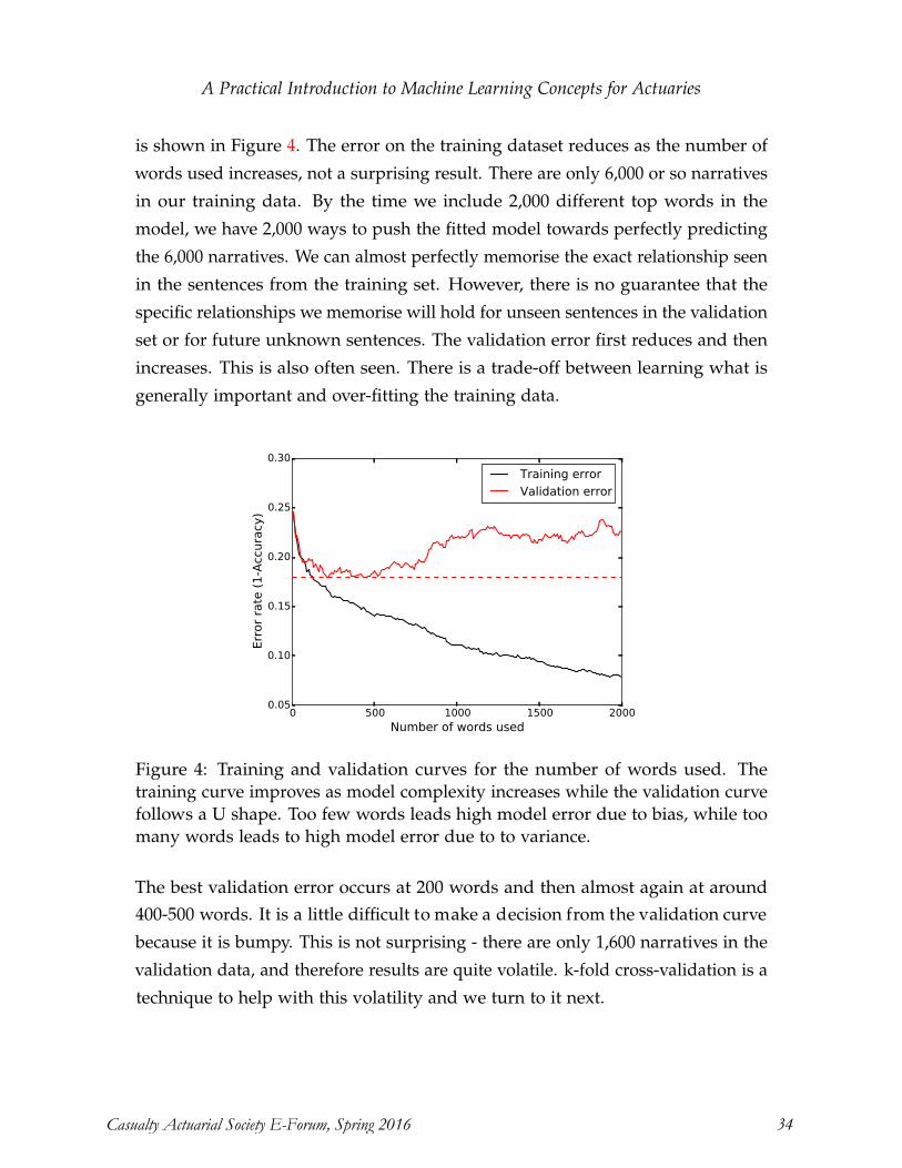
A Practical Introduction to Machine Learning Concepts for Actuaries
is shown in Figure 4. The error on the training dataset reduces as the number of
words used increases, not a surprising result. There are only 6,000 or so narratives
in our training data. By the time we include 2,000 different top words in the
model, we have 2,000 ways to push the fitted model towards perfectly predicting
the 6,000 narratives. We can almost perfectly memorise the exact relationship seen
in the sentences from the training set. However, there is no guarantee that the
specific relationships we memorise will hold for unseen sentences in the validation
set or for future unknown sentences. The validation error first reduces and then
increases. This is also often seen. There is a trade-off between learning what is
generally important and over-fitting the training data.
0 500 1000 1500 2000Number of words used
0.05
0.10
0.15
0.20
0.25
0.30
Err
or
rate
(1
-Acc
ura
cy)
Training error
Validation error
Figure 4: Training and validation curves for the number of words used. The training curve improves as model complexity increases while the validation curve follows a U shape. Too few words leads high model error due to bias, while too many words leads to high model error due to to variance.
The best validation error occurs at 200 words and then almost again at around
400-500 words. It is a little difficult to make a decision from the validation curve because it is bumpy. This is not surprising - there are only 1,600 narratives in the
validation data, and therefore results are quite volatile. k-fold cross-validation is a technique to help with this volatility and we turn to it next.
Casualty Actuarial Society E-Forum, Spring 2016 34
A Practical Introduction to Machine Learning Concepts for Actuaries
7.3 Cross-validation
In the previous section we split our first d ataset i nto t raining a nd validation datasets. This split is random and different splits would give slightly different results. This will especially be the case when the validation dataset is quite small (as for our task). Instead, we can split the first dataset into multiple ( e.g. five in this discussion) parts. We take the first p art a nd t reat i t a s a validation set and the other four parts as our training data and we carry out the process of the previous section. We then take the second part and treat it as the validation and the other four parts as our training data and we again carry out the process of the previous section. We do this for all five parts, resulting in five validation curves. Finally, we average them to get a more stable validation curve. This is called 5-fold cross-validation. In general this technique is known as k-fold cross validation (k-fold CV). k, the number of folds, is often chosen to be five or t en. We can take this to the extreme, using the same number of folds as there are examples. Then for each fold, all the training data is used except one example. This is called Leave-Out-One Cross Validation (LOOCV).
Figure 5 compares simple cross-validation with 5-fold CV. It can be seen that the curves are similar, but the 5-fold CV curve is smoother.
It is now clear that the best validation error occurs when we use around 250 words and beyond that model performance deteriorates.
7.4 Practical Tips
Training and validation curves should look sensible. If they don’t, they are probably wrong. For example, a validation curve that is below the training curve (i.e. has a lower error rate) is probably wrong.
Validation curves do not always look nicely U shaped. They can be flat, or they can reduce but not increase again. As practitioners come across such cases, they should investigate that the data, models, parameters and so on are appropriate.
A related point is whether or not we should expect the training curve to smoothly
Casualty Actuarial Society E-Forum, Spring 2016 35
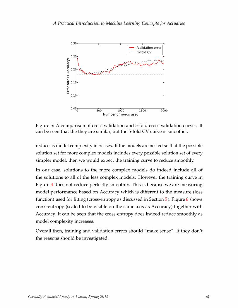
A Practical Introduction to Machine Learning Concepts for Actuaries
0 500 1000 1500 2000Number of words used
0.05
0.10
0.15
0.20
0.25
0.30
Err
or
rate
(1-A
ccura
cy)
Validation error
5-fold CV
Figure 5: A comparison of cross validation and 5-fold cross validation curves. It can be seen that the they are similar, but the 5-fold CV curve is smoother.
reduce as model complexity increases. If the models are nested so that the possible solution set for more complex models includes every possible solution set of every simpler model, then we would expect the training curve to reduce smoothly.
In our case, solutions to the more complex models do indeed include all of the solutions to all of the less complex models. However the training curve in Figure 4 does not reduce perfectly smoothly. This is because we are measuring model performance based on Accuracy which is different to the measure (loss function) used for fitting (cross-entropy as discussed in Section 5 ). Figure 6 shows cross-entropy (scaled to be visible on the same axis as Accuracy) together with Accuracy. It can be seen that the cross-entropy does indeed reduce smoothly as model complexity increases.
Overall then, training and validation errors should “make sense”. If they don’t the reasons should be investigated.
Casualty Actuarial Society E-Forum, Spring 2016 36
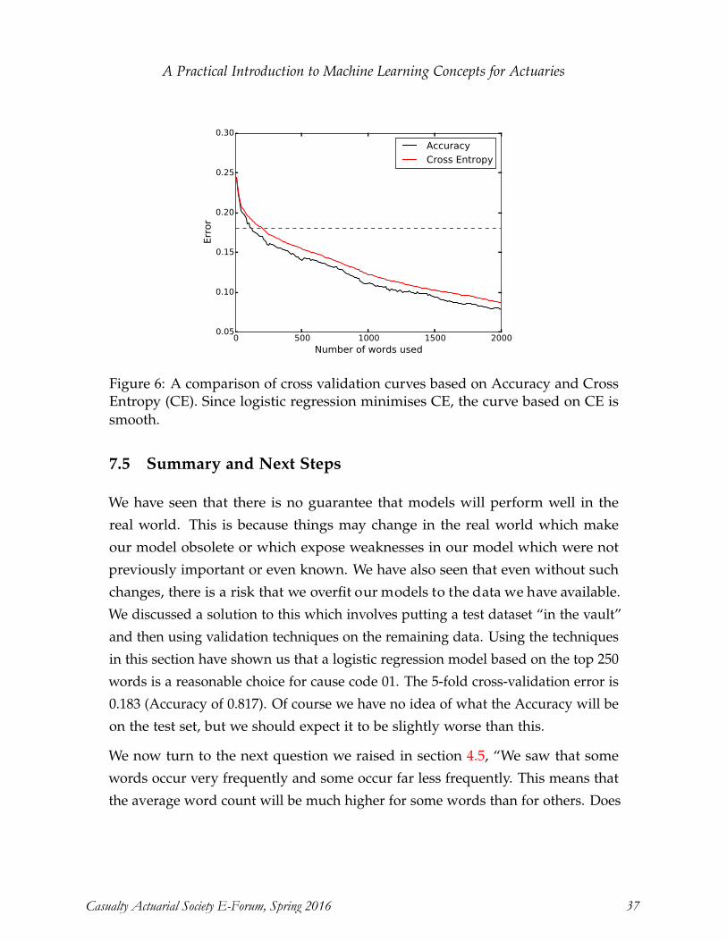
A Practical Introduction to Machine Learning Concepts for Actuaries
0 500 1000 1500 2000Number of words used
0.05
0.10
0.15
0.20
0.25
0.30
Err
or
Accuracy
Cross Entropy
Figure 6: A comparison of cross validation curves based on Accuracy and Cross Entropy (CE). Since logistic regression minimises CE, the curve based on CE is smooth.
7.5 Summary and Next Steps
We have seen that there is no guarantee that models will perform well in the real world. This is because things may change in the real world which make our model obsolete or which expose weaknesses in our model which were not previously important or even known. We have also seen that even without such changes, there is a risk that we overfit our models to the data we have available. We discussed a solution to this which involves putting a test dataset “in the vault” and then using validation techniques on the remaining data. Using the techniques in this section have shown us that a logistic regression model based on the top 250 words is a reasonable choice for cause code 01. The 5-fold cross-validation error is 0.183 (Accuracy of 0.817). Of course we have no idea of what the Accuracy will be on the test set, but we should expect it to be slightly worse than this.
We now turn to the next question we raised in section 4.5, “We saw that some words occur very frequently and some occur far less frequently. This means that the average word count will be much higher for some words than for others. Does
Casualty Actuarial Society E-Forum, Spring 2016 37
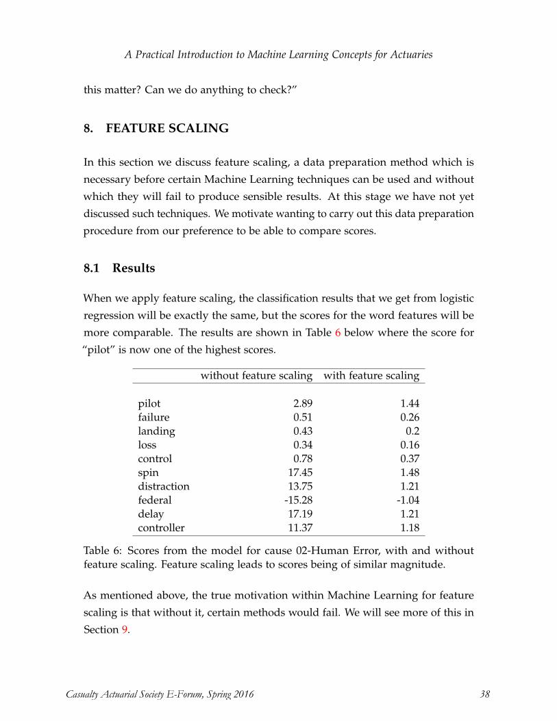
A Practical Introduction to Machine Learning Concepts for Actuaries
this matter? Can we do anything to check?”
8. FEATURE SCALING
In this section we discuss feature scaling, a data preparation method which is
necessary before certain Machine Learning techniques can be used and without
which they will fail to produce sensible results. At this stage we have not yet
discussed such techniques. We motivate wanting to carry out this data preparation
procedure from our preference to be able to compare scores.
8.1 Results
When we apply feature scaling, the classification results that we get from logistic
regression will be exactly the same, but the scores for the word features will be
more comparable. The results are shown in Table 6 below where the score for
“pilot” is now one of the highest scores.
without feature scaling with feature scaling
pilot 2.89 1.44failure 0.51 0.26landing 0.43 0.2loss 0.34 0.16control 0.78 0.37spin 17.45 1.48distraction 13.75 1.21federal -15.28 -1.04delay 17.19 1.21controller 11.37 1.18
Table 6: Scores from the model for cause 02-Human Error, with and without feature scaling. Feature scaling leads to scores being of similar magnitude.
As mentioned above, the true motivation within Machine Learning for feature scaling is that without it, certain methods would fail. We will see more of this in Section 9.
Casualty Actuarial Society E-Forum, Spring 2016 38
A Practical Introduction to Machine Learning Concepts for Actuaries
8.2 How It Works
In subsection 4.2 we saw that scores for important words that occur infrequently
are far higher than important words which occur frequently. For example, in our
training data, the word “pilot” occurs 3,429 times and has a score of 2.89 when
classifying cause 02-Human Error. On the other hand, the word spin occurs only
36 times and has a score of 18.31 when classifying cause 02-Human Error. Which
of these two words is more important to us in classifying a general example? The
score of the word “pilot” is probably high enough to tip the balance to classifying
as cause 02-Human Error in the 3,429 examples where it occurs and so it is almost
certainly more important. Thus, the fact that its score is so much lower could be
misleading.
Is it possible to change the features in such a way that their scores more closely
reflect their importance? Before adjustment, the feature for the word “pilot” is one
in the 3,429 examples where it occurs and zero otherwise. On average its value
is 0.545. Similarly, the average of the feature for the word “spin” is 0.006. We
simply adjust each feature so that on average it has a mean of zero and standard
deviation of one. We find the mean and standard deviation of each feature (across
all training examples). As we have seen, the mean of the feature for the word
“pilot” is 0.545. The standard deviation for the feature “pilot” is 0.499. In every
example we now take the feature for the word “pilot” (which is either zero or one
since there is no narrative in which the word “pilot” occurs more than once) and
deduct the mean and divide by the standard deviation. If the word ”pilot” was in
a narrative so that the feature was one, the feature becomes:
1 − 0.5450.499
= 0.91.
Applying the same process to the feature for the word “spin” leads to the value 1
being transformed to1 − 0.00573
0.0755= 13.18.
Applying a transformation to each of the features separately to make their magni-
tudes broadly similar is called feature standardisation. The particular method we
Casualty Actuarial Society E-Forum, Spring 2016 39
A Practical Introduction to Machine Learning Concepts for Actuaries
used above is sometimes called Z-score normalisation. An alternative is to ensure that each feature lies between zero and one. This can be done by deducting the minimum value and dividing by the range. (Interestingly though, this would not be useful for our data.)
8.3 Practical Tips
Feature scaling is so critical to some Machine Learning procedures, it is often built in to the programs that carry out those procedures so it is not necessary to carry it out explicitly. Clearly, one needs to know which procedures do require feature scaling and whether or not it is done automatically within the code. Explicitly carrying out feature scaling and turning off any automatic scaling within the software can lead to a more transparent process.
9. REGULARISATION
Now that we have covered loss functions and feature scaling, we are able to approach a very important idea within Machine Learning, regularisation. We will motivate this topic by referring back to our discussion in Section 7 where we found that using the most frequently occurring 250 words was optimal in terms of finding a logistic regression model which did not overfit the training data and hence generalised well. Our approach was to fit models over the top 10 words, then over the top 20 words, then the top 30 and so on. After 250 words, adding extra words increased cross validation error.
This approach has an obvious weakness. Within the setting of our task, it could well be that within the top 250 words there are words which do not help the model to generalise and indeed, there could be words amongst the many less frequent words which would help generalisation. What is more problematic is that for more general tasks, there is no obvious order at all in which to add the features. What we really need is a method that is allowed to use all the features but somehow avoids becoming too complex, leading to poor generalisation. A solution to this problem, often used in Machine Learning, is called regularisation.
Casualty Actuarial Society E-Forum, Spring 2016 40
A Practical Introduction to Machine Learning Concepts for Actuaries
9.1 Results
For cause 02-Human Error, the best 5-fold cross validation error (error of 0.183, Accuracy of 0.817) was previously achieved with the top 250 most frequently occurring words. If, instead, we use the top 5,000 words, but control model complexity using a type of regularisation called L2 regularisation, the best 5-fold cross validation error is reduced to 0.173 (and Accuracy increases to 0.827). This does not guarantee that when we finally take the test dataset out of the vault, the regularised model will perform better, but an improvement of 1% for little extra modelling effort is worthwhile in our context (where the naive model achieves 75% Accuracy).
When we carry out regularisation, we only accept more complex models if they provide a reasonable improvement in model performance on the training set. The amount of performance improvement needed in order to accept a more complex model is controlled by a parameter. We will explain in further detail below that the optimal value for this parameter can be found using cross validation. Figure 7 shows the result of this search. It can be seen that as the parameter allows models of increasing complexity (increasing values on the x-axis), we first see improvement on validation error, but when the parameter allows the models to get too complex, validation error suffers.
We will also discuss below a form of regularisation called L1 regularisation. We will explain that this has the nice property that it will set many of the βs to zero. When β is zero for a feature, the word relating to that feature is not being used at all in the model. Hence, L1 regularisation selects which words are important out of the full vocabulary of words that we choose to use. When we used a vocabulary of the top 5,000 words with L1 regularisation, the number of words used in the fitted model for cause 01-Aircraft was 1,244 (though model validation error was not as good as under L2 regularisation).
Casualty Actuarial Society E-Forum, Spring 2016 41
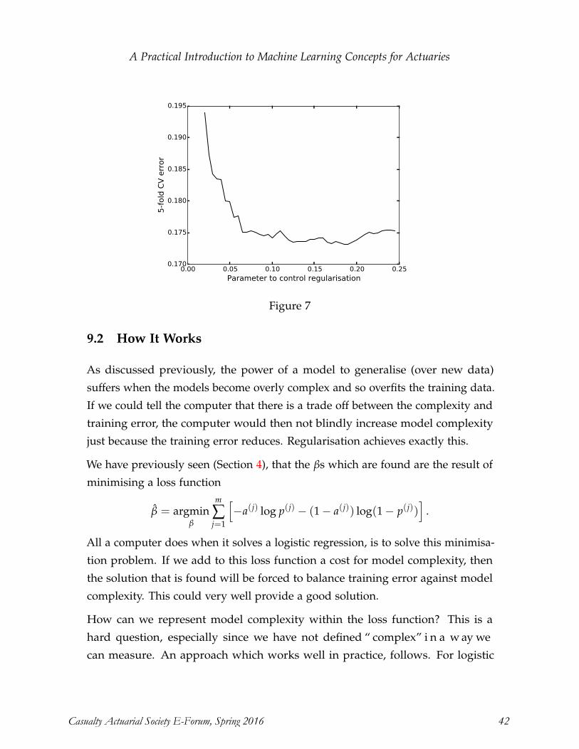
A Practical Introduction to Machine Learning Concepts for Actuaries
0.00 0.05 0.10 0.15 0.20 0.25Parameter to control regularisation
0.170
0.175
0.180
0.185
0.190
0.195
5-f
old
CV
err
or
Figure 7
9.2 How It Works
As discussed previously, the power of a model to generalise (over new data)
suffers when the models become overly complex and so overfits the training data.
If we could tell the computer that there is a trade off between the complexity and
training error, the computer would then not blindly increase model complexity
just because the training error reduces. Regularisation achieves exactly this.
We have previously seen (Section 4), that the βs which are found are the result of
minimising a loss function
β̂ = argminβ
m
∑j=1
[−a(j) log p(j) − (1 − a(j)) log(1 − p(j))
].
All a computer does when it solves a logistic regression, is to solve this minimisa-
tion problem. If we add to this loss function a cost for model complexity, then the solution that is found will be forced to balance training error against model complexity. This could very well provide a good solution.
How can we represent model complexity within the loss function? This is a hard question, especially since we have not defined “ complex” i n a w ay we can measure. An approach which works well in practice, follows. For logistic
Casualty Actuarial Society E-Forum, Spring 2016 42
A Practical Introduction to Machine Learning Concepts for Actuaries
regression, consider the values for the βs. If there are lots of βs with non-zero
values, the model is complex. We might try simply adding the values of all the βs
and using this value to reflect model complexity, but then positive and negative
values will cancel out. The most obvious alternatives are to add the squared values
or the absolute values. If we use the sum of the squared values, the problem is
now simply to find:
β̂ = argminβ
[m
∑j=1
[−a(j) log p(j) − (1 − a(j)) log(1 − p(j))
]+ λ
n
∑i=1
β2i
].
where we have also introduced a new parameter λ which controls the trade-off between model complexity and training error.
Regularisation using the squares of the βs is known as L2 regularisation. Regulari-
sation using the absolute values of the βs is called L1 regularisation and is known as the LASSO (Least Absolute Shrinkage and Selection Operator). Although we do not give the reason here, using the LASSO has the interesting outcome that many of the βs will be zero.
There is an important issue that arises when trying to implement the above. λ provides a trade-off between model complexity and training error. We decided to measure model complexity based on the size of the βs but the βs are not really unique. They depend on the scale of the features. If we measure a feature using centimetres, the β for that feature will be far smaller than if we measure that feature in kilometres. Results of regularisation, therefore, depend on the possibly arbitrary scale of the features. To deal with this, some form of feature scaling is always recommended before carrying out regularisation (unless all features are of a similar scale).
Finding solutions to regularised logistic regression is straightforward other than finding the best trade off between model complexity and training error, i.e., the best value for λ. Since λ is a hyper-parameter, as with the parameter for the number of words in Section 7, we find it using cross validation. We simply try a range of values for λ and for each we fit the regularised model on training data and find the validation error. The result of this process is shown in Figure 7 and
Casualty Actuarial Society E-Forum, Spring 2016 43
A Practical Introduction to Machine Learning Concepts for Actuaries
has already been discussed above. We note, however, that the values on the x-axis
are in fact 1λ often referred to as C. This allows increasing values on the x-axis to
represent increasing model complexity.
9.3 Practical Tips
Often, the curve produced whilst searching for the optimal model complexity
will reduce quickly and then be flat over a long range. It may be that the very
best cross-validation error is achieved when the model is quite complex, but a
validation error almost as good is achieved earlier on using a much simpler model.
Given the downsides of using more complex models, it is probably better to use
the simpler model. Ad-hoc methods to chose the appropriate model complexity
exist, but the main idea is to use a well reasoned approach (and not to be tempted
to see performance on the test dataset).
10. FEATURE ENGINEERING
In this section we apply regularisation to help us explore further feature engi-
neering. We create features which we think likely to improve model performance
and use k-fold cross-validation, logistic regression and regularisation to decide
whether or not to include the new features. We find that if too many features are
added, regularisation does not find the best model. However, with some care,
model performance (as measured by Accuracy using 5-fold cross validation) does
improve.
10.1 n-grams
Bi-grams are phrases of two words and tri-grams are phrases of three words.
Consider the narrative:
The failure of company maintenance personnel to ensure that the airplane’s nose baggage door latching mechanism was properly config-
ured and maintained, resulting in an inadvertent opening of the nose
Casualty Actuarial Society E-Forum, Spring 2016 44

53
A Practical Introduction to Machine Learning Concepts for Actuaries
baggage door in flight.
In this narrative, bi-grams are, “the failure”, “failure of”, “of company”, “company maintenance”, “maintenance personnel”, “personnel to” and so on. Tri-grams are “the failure of ”, “failure of company”, “of company maintenance” and so on.
Rather than simply taking all bi-grams and tri-grams, we take only those that occur more frequently than would happen by chance given the frequency of their constituent words. For example, out of 226,340 words in the narratives, the word “go” appears 25 times and the word “around” appears 36 times. Were they to appear independently of each other, the phrase “go around” would be very unlikely to appear even once, yet it appears 22 times.
The bi-grams chosen in this manner include: go around, timely manner, avia-
tion administration, dynamic rollover and situational awareness, which are all clearly meaningful. The tri-grams chosen in this manner include: federal aviation administration and instrument meteorological conditions and other meaningful phrases.
In the same way, quad-grams are phrases of four words and included phrases such as “loss of engine power”.
Initial results from using bi-grams and tri-grams as features were disappointing, Accuracy did not improve. Adding quad-grams to this extended feature set also showed no improvement. However when we kept the original features (based on frequently occurring words) and added quad-grams only, performance improved from an Accuracy of 82.7% to 84.1%.
10.2 Lexical Diversity
Lexical diversity measures the diversity of words used in a text. We define it here as the number of words in the text divided by the number of unique words in the text. A low value implies a large diversity of words and the minimum it can be is one. For example, in the sentence “The animal ate the animal.” there are 5 words but only 3 unique words, so the lexical diversity is = 1.67.
Casualty Actuarial Society E-Forum, Spring 2016 45
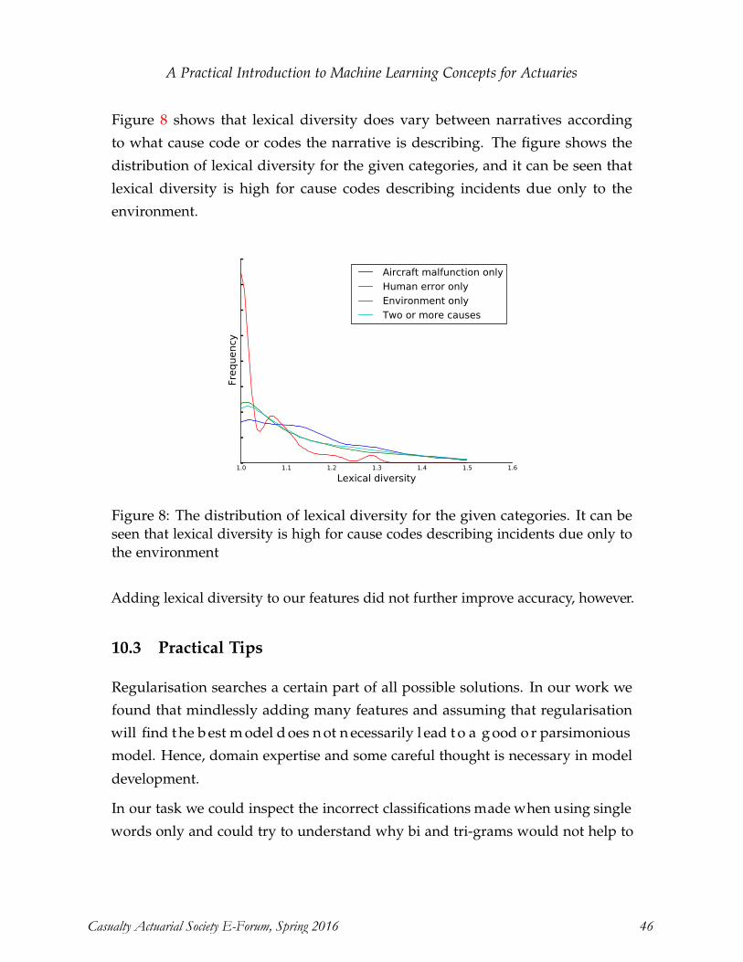
A Practical Introduction to Machine Learning Concepts for Actuaries
Figure 8 shows that lexical diversity does vary between narratives according
to what cause code or codes the narrative is describing. The figure shows the
distribution of lexical diversity for the given categories, and it can be seen that
lexical diversity is high for cause codes describing incidents due only to the
environment.
1.0 1.1 1.2 1.3 1.4 1.5 1.6
Lexical diversity
Frequency
Aircraft malfunction only
Human error only
Environment only
Two or more causes
Figure 8: The distribution of lexical diversity for the given categories. It can be seen that lexical diversity is high for cause codes describing incidents due only to the environment
Adding lexical diversity to our features did not further improve accuracy, however.
10.3 Practical Tips
Regularisation searches a certain part of all possible solutions. In our work we found that mindlessly adding many features and assuming that regularisation will find t he b est m odel d oes n ot n ecessarily l ead t o a g ood o r parsimonious model. Hence, domain expertise and some careful thought is necessary in model development.
In our task we could inspect the incorrect classifications made when using single words only and could try to understand why bi and tri-grams would not help to
Casualty Actuarial Society E-Forum, Spring 2016 46
A Practical Introduction to Machine Learning Concepts for Actuaries
correct those errors. In a more general setting such as predicting claims frequency there would be no obvious way to understand why certain extra features are not helpful. Nevertheless, it is important to be honest, however much we might think that a feature should be useful. If it is not, we need to admit that there is no support for our hypothesis in the data. Incidentally, this does not mean we cannot use the feature as a rating factor, only that we should note in our model documentation that we have chosen to use something which is not supported by the data and which could, therefore, potentially harm model performance.
10.4 Summary and Next Steps
We have now covered many of the key Machine Learning ideas relevant for creating a proper structure for applying Supervised Learning techniques. Feature scaling and regularisation allow us to fit m odels w here t here m any features, whilst limiting the risk of overfitting. F eature e ngineering p rovides a way to improve model performance - if good features can be found. Splitting our data into training, validation and test datasets and using the test dataset only at the very end of all model fitting r educes t he r isk o f o ver-fitting an d po or model performance (generalisation error). With this structure in place, the natural next steps in our analysis are the application of techniques from traditional Natural Langauge Processing as well as more recent Machine Learning based ideas (such Gradient Boosting and Deep Neural Networks) in order to try to improve model performance. This however, is beyond the scope of this paper and instead we now conclude by taking the test data “out of the vault” and finding the model with the lowest generalisation error.
11. CONCLUSIONS
11.1 Model Comparison
Since we have been very careful not to use our test set for any part of the fitting on any of the models, we can now, finally, take our test set out of the vault and
Casualty Actuarial Society E-Forum, Spring 2016 47
A Practical Introduction to Machine Learning Concepts for Actuaries
measure performance of the various models. We can be reasonably sure that, so
long as recording practice at the NTSB does not change and the distribution of the
types of accident do not change, the accuracy of our methods on the test set will
reflect accuracy on future, as of yet unseen, examples. Table 7 shows the results.
Model description 5-fold testcross validation
Logistic regression (top 500 words) 81.0% 81.3%Logistic regression (top 250 words) 81.7% 81.3%Logistic regression (5000 words and regularisation) 82.7% 83.2%As above but 1250 words and 4-grams 84.1% 83.8%Gradient Boosting (using trees of depth 4) 83.4% 83.5%BoosTexter 83.8% 82.8%
Table 7: 5-fold cross-validation and test set Accuracy for the various models inthis paper.
Logistic regression using the 1,250 words chosen from an earlier model together
with 4-grams performs best on the test set. Although this model is more complex
than some of the earlier models, the performance improvement on the test set is
significant, and therefore, we chose to proceed with this model.
It is of interest to see which cases the model does not correctly classify. Over half
of cases incorrectly classified would probably have been classified the same by a
human being using the same narrative. For example:
The ground crewman’s failure to follow the tow bar disconnect stan-
dard operating procedures.
is classified by our predictor as not being due to cause 0 1-Aircraft. However, the NTSB code does flag this c ause. The reason for this could be that the extended narratives, which we have not used, contain additional information. Beyond this, the models remain imperfect because they consider words such as “failure” out of context, that is, without knowing whether the narrative refers to pilot failure of a failure of some part of the aircraft. Domain specific Natural Language models or modern forms of Neural Networks would be expected to provide improved performance in this task.
Casualty Actuarial Society E-Forum, Spring 2016 48

A Practical Introduction to Machine Learning Concepts for Actuaries
11.2 Conclusions
Machine Learning techniques for Supervised Learning are very easy to apply in
practice. Open-source and proprietary software make using the most modern
techniques as easy as fitting a generalised linear model. However, with increased
model complexity comes the risk of choosing models that will actually perform
more poorly in practice.
The concepts we have discussed:
• the loss function
• choosing a model evaluation metric deliberately rather than by default
• using training, validation and test sets to correctly understand model gener-
alisation error
• using feature engineering to enrich the data
• using feature scaling to ensure correct fitting of certain model types
• and using regularisation together with cross validation to find the best of a
set of models
are key parts of the model building pipeline that is required for the fitting and choosing of appropriate models. Where not already done so, these can be easily integrated to the work flow of actuarial teams.
Acknowledgement
The authors gratefully acknowledge the the support provided by Mazars which enabled the modelling underlying this paper to be undertaken.
Biography of the Authors
Alan Chalk is a freelance Actuary with experience in predictive analytics and Data Science. He is a Fellow of the Institute of Actuaries and has Masters Degrees in Statistics and in Machine Learning. He can be contacted at: [email protected].
Casualty Actuarial Society E-Forum, Spring 2016 49

A Practical Introduction to Machine Learning Concepts for Actuaries
REFERENCES
[1] Trevor J. Hastie, Robert John Tibshirani, and Jerome H. Friedman. The elements
of statistical learning : data mining, inference, and prediction. Springer series in
statistics. Springer, New York, 2 edition, 2009.
Casualty Actuarial Society E-Forum, Spring 2016 50