Catching the agent on the wrong foot: ex post choice of monitoring

Journal of Public Economics 82 (2001) 327–347www.elsevier.com/ locate /econbase

Catching the agent on the wrong foot: ex post choice ofmonitoring

a a,b ,*´Fahad Khalil , Jacques LawarreeaDepartment of Economics, Box 353330, University of Washington, Seattle, WA 98195, USA

bECARES, Avenue Roosevelt, SO-CPI 114-1050 Brussels, Belgium

Received 4 November 1999; received in revised form 2 October 2000; accepted 17 October 2000

Abstract

In a principal-agent model with multiple performance measures, we show that theprincipal benefits by choosing ex post which variables will be monitored. If it is too costlyfor one type of agent to mimic all performance measures expected from another type, theprincipal can hope to catch the agent on the wrong foot if the agent tries to misrepresent histype. For cases of small asymmetry of information, the principal can implement the firstbest contract. For more serious asymmetries of information, the first best is not implement-able. Then the low type may be required to overproduce, which is in contrast to thetraditional result of second best contracting. We also obtain a ranking of monitoringinstruments according to the frequency of their use. 2001 Elsevier Science B.V. Allrights reserved.

JEL classification: D23; D82; L22

1. Introduction

In a principal agent problem under adverse selection, a principal can often findmany performance measures to screen an agent and provide incentive. If the agentknows the variables that are being monitored, an agent of one type can obtain rentby mimicking the contractual obligation of another (inferior) type. In what has

*Corresponding author. Tel.: 11-206-543-5632; fax: 11-206-685-7477.É-mail address: [email protected] (J. Lawarree).

0047-2727/01/$ – see front matter 2001 Elsevier Science B.V. All rights reserved.PI I : S0047-2727( 00 )00148-1

´328 F. Khalil, J. Lawarree / Journal of Public Economics 82 (2001) 327 –347

been touted as the biggest accounting fraud ever ($19 billion), the Securities andExchange Commission (SEC) has recently investigated a company called CUCInternational. It is alleged that the company fooled auditors from Ernst and Youngby faking the numbers of some of its subsidiaries. ‘‘The SEC says that the fraudwas easier to pull off because CUC officials knew which subsidiaries would beaudited, and therefore hid the most obvious frauds in subsidiaries that they knewthe auditors would not look at.’’ (New York Times, June 16, 2000).

It is standard in the literature to assume that the principal announces ex ante1which performance measures will be used. In this paper, we show that the

principal could gain by choosing ex post which variables will be monitored. If it istoo costly for one type of agent to mimic all performance measures expected fromanother type, the principal can hope to catch the agent on the wrong foot if theagent tries to misrepresent his type.

There are many examples where different measures of performance can be usedto address an agency problem under adverse selection. Revisiting the standardtaxation model of Mirrlees (1971), Maskin and Riley (1985) point out that a taxauthority can use various instruments, such as input and output, to derive theoptimal tax scheme. In regulation theory, the optimal scheme for a monopolist canalso be based on various signals such as input, output, costs, etc. (Caillaud et al.,1988). An important issue in pollution control is the choice between emissiontaxes and taxes on other factors of production that are correlated with emissions(see Besanko, 1994; Lewis, 1996; Schmutzler and Goulder, 1997). The taxauthority must therefore choose between monitoring emission directly or, alter-natively, monitoring the pollution abatement technologies (e.g., end-of-pipetechnology) installed by the polluting firm.

Analyses of multiple performance measures also appear in fields other thanpublic economics. Lafontaine and Slade (1996, 1998) argue that, in mostmanufacturer–retailer relationships including franchising, the manufacturer canmonitor the retailer through sales data or through more direct signals of effort, e.g.,by tasting the food quality, assessing the cleanliness of the unit or by determiningwork hours. In a similar vein, Anderson and Oliver (1987) distinguish betweenbehavior-based compensation and outcome-based compensation. In labor econ-omics, the literature on piece-rate vs. wage-rate is another illustration of the

ávailability of multiple signals (see Matutes and Regibeau (1994) for a recent2contribution).

Even when the principal receives several signals, if mimicking is costless, theagent simply mimics every possible performance measure so that misrepresenta-tion is never detected. Therefore, the principal may not be able to improve thecontract by increasing the number of signals in this case. However, if mimicking is

1See for example, Baron and Myerson (1982), Sappington (1983), and Laffont and Tirole (1993).2There is also a vast literature on agricultural contracts where wage contracts are input (labor hours)

based, and sharecropping is output based. See Singh (1989).

´F. Khalil, J. Lawarree / Journal of Public Economics 82 (2001) 327 –347 329

costly, then increasing the potential number of signals raises the agent’s cost ofmisrepresenting his type. This would necessarily help the principal if signals were

3free to observe. Since performance measures are typically costly to obtain,4increasing the number of signals is costly to the principal. However, this is based

on the implicit assumption that all the signals announced ex ante are indeedmonitored eventually. Under ex post monitoring, the principal announces a largenumber of variables ex ante, but only decides ex post which ones he will actuallymonitor. This gives the principal the option of monitoring only a subset of thevariables and save on monitoring cost while using the incentive power of a largenumber of variables.

We want to emphasize that the principal may collect or create an access to alarge amount of data, even if verifying all of them is too costly. For income taxreturns, the tax code requires taxpayers to report many items that can be

5crosschecked if the IRS wants to do so. In life insurance contracts, individuals areasked to answer a large number of questions regarding their health. Forcompliance with the chemical weapons treaty, participating countries have to makevery detailed announcements regarding production plans of every chemical plant

6in the country. Similarly, immigration officials ask a long list of questions whenforeigners apply for a US visa. In each of these examples, what is important is thatthe principal reserves the right to decide ex post which pieces of information toverify.

If the number of variables announced ex ante is large, mimicking everyperformance measure may become too costly for the agent. As a consequence, theagent trying to mimic another type has to guess which variables will actually bemonitored. If he guesses incorrectly the agent will be caught on the wrong foot andpenalized since his true type will then be revealed. This threat of a penalty reducesinformation rent, and for small cases of asymmetry of information, the principal

7can implement the first best contract.Our analysis may have important empirical implications in that actual rent in

3 ¨See Holmstrom (1979) in the context of moral hazard and Rochet and Stole (2000) in the context ofmultidimensional screening.

4While more information is typically better, the principal might not use all the available variables.The reason could be that these variables are costly to observe or simply that it is too costly to make allof them verifiable. Such an instance would be common when the output has a quality component, andan expert witness has to convince a third party of the true value of the quality parameter. This sameassumption is at the root of the incomplete contract literature (see Hart, 1995). Dewatripont and Maskin(1995) also show that observing more than one variable is not necessarily better when renegotiation is

állowed after one variable has been revealed and before the other one is revealed. Cremer (1995) isanother example of such an effect of revealing information too early in a repeated relationship.

5Bruce (1998, p. 472) presents a nice example where the IRS caught pizza parlors committing taxfraud. The IRS auditors showed inconsistencies in the reports of input (flour) and output (sales).

6See the web site http: / /www.opcw.nl / for more details on the treaty.7In Section 2, we contrast our approach with the traditional auditing model after presenting our

model.


real world contracts may be much less than what would be inferred from a modelbased on one monitoring variable. In reality, organizations have access to multiplemonitoring variables even though explicit incentives may primarily be based onone variable. Therefore the scope for misrepresentation may be quite limited. Intheir survey paper, Andreoni et al. (1998, p. 821) claim that the IRS’s use of‘informational reporting,’ which requires reports on multiple items in tax returns,could partly explain why compliance levels have been so high even thoughpenalties and probabilities of auditing are relatively low. Our results suggest policyguidelines as they establish the notion that the access to a menu of variablesimplies more efficient contracts than if only one variable was available.

The choice between monitoring variables has attracted attention in the recentliterature on incentive problems due to hidden information. Maskin and Riley(1985) introduce the problem of input versus output monitoring in this framework,

8and show that output monitoring is better. In a similar vein, Lewis and Sappington(1995), consider the case of pollution control, and ask if monitoring pollution or

´monitoring abatement equipment is more efficient. Khalil and Lawarree (1995)extend the work of Maskin and Riley, and show that the choice of the monitoringinstrument depends on whether the principal or the agent collects the output.Barzel (1997) studies a similar problem in the context of moral hazard. In a recentpaper, Bontems and Bourgeon (2000) show that even the choice of the monitoringinstrument can be used as a screening device. The principal lets the agent choosethe instrument. They show that some types may choose input while others maychoose output monitoring, and in some cases even the first best efforts can beimplemented. However, this literature assumes that the agent knows the variable tobe monitored before he acts, whereas we let the principal choose this variable afterthe productive action has occurred. The literature on multi-dimensional screening(see Rochet and Stole, 2000 and references therein) is also related. Whereas thisliterature assumes that signals are observed for free, we assume that it is costly tomonitor signals. Indeed, our main point is that when signals are costly, theprincipal can save on monitoring cost by only observing a subset of signals whilederiving benefit from all of them.

To illustrate our ideas, we use a model similar to Maskin and Riley (1985)where the principal can monitor either input or output. In addition to the result offirst best contract for cases of small asymmetry of information, we find that theprincipal may ask a low type agent to overproduce as opposed to the traditionalunder-production result. Also, we obtain a ranking of instruments even when inputand output monitoring are equally costly and equally accurate: the principal willmonitor input more often.

The paper is organized as follows. We introduce the model in Section 2. Twobenchmark contracts are presented in Section 3: the full information contract, and

8For an earlier treatment, see Wittman (1977).


the contract under ex ante choice of monitoring. Our main results are presented inSection 4, while we explore some extensions in Section 5 and present ourconclusions in Section 6.

2. The model

A risk neutral principal hires a risk neutral agent to work for him. The agent’sinput e $ 0 along with his productivity parameter u determines output X5a(e, u ),with a(0, u )$0, a .0, a .0, a # 0, a $ 0, lim a (e, u ) 5 `. While wee u ee eu u →` e

refer below to input e as effort, it could also include non-effort related decisionssuch as the types of input purchased or the end of pipe pollution controltechnology adopted or the marketing strategies selected. Effort cost is inversely

9related to productivity. The cost of effort for type u is given by the function c(e,u ), with c .0, c .0, c ,0, c ,0, c(0, u )50, lim c (e, u ) 5 `, lime ee u eu e→` e e→0

c (e, u ) 5 0, lim c(e, u ) 5 lim c (e, u ) 5 0.e u →` u →` e

For simplicity, we assume that productivity can be either high (u ) or low (u ),2 110

u .u . 0. The parameter u is private information of the agent. The principal’s2 1

subjective probability that u 5u is q. We assume that it is optimal for the1

principal to employ either type of agent. This implies that q is not too small giventhe ratio u /u .2 1

A contract is a six-tuple he , e , t , t , v , v j, where v is the probability of1 2 1 2 1 2 i

output monitoring when the agent announces that he is of type i and t is thei

corresponding transfer. Note that the contract also implicitly specifies output levelsfor each type. For instance, if type u is supposed to put in effort e in exchange1 1

for t , then the output implied by the contract is: X 5a(e , u ). The principal can1 1 1 1

either monitor the input (e) or the output (X). Monitoring is perfect but publiclyreveals only the variable that is monitored, e.g., if output is monitored, X isperfectly known but not e nor u. This leaves room for one type to mimic the other.If X is observed, it cannot be ruled out that the high type has mimicked the low1

type. If e is observed, it is not known whether output is X 5 a(e , u ) . X . Even1 1 2 1

though the principal collects the output, we assume that, under input monitoring,he cannot observe output or make it verifiable. There are many examples whereoutput has features, such as quality, that are difficult to observe even though thebeneficiary of the output is clear. When controlling pollution, the EPA, represent-ing citizens, ‘consumes pollution’ but does not observe its level unless it monitorsit (see Swierzbinski (1994)). Healthcare authorities, like Medicare, contract withhealthcare providers, but the benefit of treatment accrues to patients and is

9The previously discussed paper by Bontems and Bourgeon (2000) shows that the oppositeassumption leads to the introduction of countervailing incentives.

10Assumptions made above regarding the functions a(.) and c(.) have obvious counterparts for thisdiscrete framework.


typically not observed by the authorities (see Chalkley and Malcomson, 1999). Itis difficult to evaluate the work of an auto mechanic, and the military may never

11learn the efficacy of weapons in a nuclear war.Differentials in cost and precision between input and output monitoring have

straightforward consequences in our model. The principal would always be biasedtowards the cheaper and more precise monitoring instrument. To focus on aranking of instruments based only upon incentives, we therefore assume that inputand output monitoring are equally costly and equally precise. Monitoring is errorfree and it costs C to monitor either input or output. A more critical assumption isthat it is not feasible to monitor both input and output. This assumption capturesthe fact that in general it is too costly for the principal to monitor every possibleperformance measure. In our model, if both input and output were observed, thefirst best (minus 2C) would always be reached. We could also have allowed theprincipal to choose to observe neither input nor output. If nothing was observed,the transfer would be based only on the agent’s announcement and the expected

12cost of monitoring would drop below C.We assume that the principal can commit to the probability of monitoring as

part of the contract. This assumption turns out to be innocuous in our model sincewe assume that the principal must monitor either input or output, which can beobserved with equal precision and accuracy. More generally, the commitmentassumption is restrictive, but is used frequently in models with monitoring. It istypically justified using informal arguments from repeated games or delegationgames. Melumad and Mookherjee (1989) model IRS audits to show that if thepublic can observe some aggregate variables like the IRS budget, aggregate costsand fines collected, then the government can attain the full commitment outcome

13even if it cannot control audit probabilities directly. In a model withoutcommitment to the monitoring probability, the equilibrium would be in mixedstrategies (see for example Khalil, 1997), and the optimal contract would be morecomplex to characterize. Since our goal was to demonstrate simply the benefit ofbasing the contract on multiple signals while monitoring only a subset, we chosethe simpler model with commitment.

The principal collects the output and compensates the agent with a transfer t.The agent receives the transfer t, but bears the cost c(e, u ). The agent knows hisproductivity before signing the contract. Therefore he must receive his reservation

11 ´See Lewis-Sappington (1991), Lawarree-Van Audenrode (1996) or Strausz (1997) for furtherexamples.

12In tax-compliance models (e.g. Mookherjee and Png’s, 1989) tax is only based on reported incomeunless there is an audit. In Swierzbinski’s (1994) model of pollution control, the regulatory policy isbased on the announced type unless the level of pollution is monitored. But in each case the principalannounces ex ante the variable to be monitored.

13One could interpret the formula for computing DIF scores (see Andreoni et al., 1998) as an attemptat coordinating actions of IRS auditors, and thus a form of commitment to auditing. Even though theformula is secret, it presumably can be inferred over time.


utility (normalized to zero) in any state of the world. The agent is asked toannounce his type after accepting the contract. If the monitored signal does notcorrespond to the announcement, shirking is detected and the agent does notreceive any transfer. The penalty for shirking is therefore the uncompensated cost

14of effort . A more stringent penalty could also be considered: besides losing histransfer the agent may be required to suffer an additional fine F .0. For now, weassume that F50, and we will discuss the case of F .0 later. To summarize, wepresent below the timing:

We have presented a model in which the principal can hope to catch the agenton the wrong foot and penalize him by choosing the monitoring variables ex post.The agent could not be penalized in a model of ex ante choice or if mimicking iscostless. With ex ante choice, the agent knows which variables to mimic. Withcostless mimicking, the agent would mimic every variable. In either case,misrepresentation cannot be detected; it can only be deterred by giving rent, andthere are no penalties on or off the equilibrium path. The monopoly regulationmodel of Baron and Myerson (1982) is an example with ex ante choice andcostless mimicking. Sappington (1983) is another example of ex ante choice andcostless mimicking, but with multiple signals. The model of input versus outputmonitoring used here is due to Maskin and Riley (1985), and it provides a cleanway to capture the impossibility of mimicking every variable in a simpletechnology: when one type of agent mimics another, he can mimic another type’sinput or output but not both. In Section 5, we extend our model to allow the agentto mimic every variable by introducing falsification cost.

Our main ideas would generalize to a model with more than two types. Considerfor instance a continuum of types. The agent must still announce his type andmisrepresentation will be detected in the same fashion. The only difference is that,when misrepresentation is detected, the monitored variable could correspond to the

15level of another existing type. However, the agent still gets caught since themonitored variable does not correspond to the equilibrium value of the announcedtype.

In our model, efficiency of the optimal contract is enhanced by off-the-

14Following Laffont-Tirole(1993), we also interpret the agent’s limited liability as the principal’sinability to extract money.

15In our model with two types, when the high type agent mimics the input of the low type heproduces an output higher than the equilibrium output of the low type and lower than the equilibriumoutput of the high type.


equilibrium path penalties. This aspect of our model is similar to auditing modelswhere the principal can commit to audit probabilities. However, our model differs

16from the traditional auditing model. In these models, one variable, say output, isalways observed, and therefore a high type may shirk by producing the outputlevel of a low type. In order to discover shirking, the principal has to observe asecond variable (input), which is the outcome of an audit. In our model, theprincipal has access to two variables, but ultimately observes only one variable. Ifthe principal randomizes between the potential monitoring variables, a shirkingagent faces a positive probability of penalty even if only one variable is observed.Thus monitoring cost may be lower than under auditing since only one variablehas to be monitored in equilibrium.

3. The first best contract, and the contract under ex ante choice ofmonitoring

If the agent’s type is publicly observable, the principal’s problem is to chooseefforts and transfers for each type of agent to maximize expected profit:

q[a(e , u ) 2 t ] 1 (1 2 q)[a(e , u ) 2 t ]1 1 1 2 2 2

subject to the individual rationality constraints of the two types:

(IR1) t 2 c(e , u ) $ 0,1 1 1

(IR2) t 2 c(e , u ) $ 0.2 2 2

The solution is the first best contract, where marginal benefit of effort equalsmarginal cost, and there is no rent. For i51, 2,

* *a (e , u ) 5 c (e , u ),e i i e i i

* *t 5 c(e , u ).i i i

Next, we examine the case where the agent’s type is private information and theprincipal commits to monitor a particular variable as part of the contract (that is,v 50 or 1). Under input monitoring, transfers are based on observed input, andi

the incentive compatibility constraints are:

ICi1 t 2 c(e , u ) $ t 2 c(e , u ),s d 1 1 1 2 2 1

ICi2 t 2 c(e , u ) $ t 2 c(e , u ).s d 2 2 2 1 1 2

16 ´See for example, Baron and Besanko (1984) or Kofman and Lawarree (1993) for auditing modelswith commitment, and Khalil (1997) for the case without commitment. Without commitment, theremay be penalties in equilibrium.


On the other hand, under output monitoring, payments are based on observedoutput, and the incentive compatibility constraints now become:

˜ICo1 t 2 c(e , u ) $ t 2 c(e , u ),s d 1 1 1 2 2 1

˜ICo2 t 2 c(e , u ) $ t 2 c(e , u ),s d 2 2 2 1 1 2

˜ ˜ ˜ ˜where e and e satisfy a(e , u )5a(e , u ) and a(e , u )5a(e , u ). Indeed,1 2 1 2 1 1 2 1 2 2

when mimicking the low type, the high type agent has to produce X and exert an1

˜effort e smaller than e . The low type mimicking the high type must exert an1 1

˜effort e higher than e .2 2

The principal’s problem is to maximize expected profit subject to the individualrationality constraints, and the relevant incentive compatibility constraints given

´the monitoring scheme. In Khalil-Lawarree (1995), we show that input monitoringyields higher profit to the principal in this model. Intuitively, it is because theagent receives rent from two sources under output monitoring and from only onesource under input monitoring. The rents for the high type agent under input andoutput monitoring are respectively,

IRent 5 c(e , u ) 2 c(e , u ),1 1 1 2

O ˜Rent 5 c(e , u ) 2 c(e , u ).1 1 1 2

OThe expression for Rent shows that the high type agent receives a rent because˜(i) he can exert a lower level of effort (e , e ) and (ii) he has a lower cost of1 1

effort. Under input monitoring, the agent only commands a rent from a lower costof effort. The other results are standard: the high type produces efficiently; the lowtype under-produces and his effort is inversely related to u /u ; the low type does2 1

not earn rent.

4. Ex post choice of monitoring

We now return to the case where the principal does not have to decide toexclusively monitor input or output before the effort is taken. The principal cancommit to a probability of output monitoring v [[0, 1]. The principal’s problemi

is to choose a contract that solves the following problem (P):

Max q[a(e , u ) 2 t ] 1 (1 2 q) [a(e , u ) 2 t ] 2 C1 1 1 2 2 2

s.t.˜(IC ) t 2 c(e , u ) $ maxhv t 2 c(e , u ), (1 2 v )t 2 c(e , u )j,2 2 2 2 1 1 1 2 1 1 1 2

˜(IC ) t 2 c(e , u ) $ maxhv t 2 c(e , u ), (1 2 v )t 2 c(e , u )j,1 1 1 1 2 2 2 1 2 2 2 1

(IR ) t 2 c(e , u ) $ 0,2 2 2 2

(IR ) t 2 c(e , u ) $ 0.1 1 1 1


While the individual rationality constraints are standard, the incentive com-patibility constraints require elaboration. We explain (IC ) only since (IC ) is2 1

analogous. A high type agent can claim to be a low type either by mimicking˜input, i.e., exerting e , or by mimicking output, i.e., exerting e . If he chooses e ,1 1 1

he only receives t if input is monitored, which occurs with probability (12v ),1 1

˜while he bears the cost c(e , u ) for certain. If he chooses e , he will only receive1 2 1

˜t with probability v , while bearing the smaller cost c(e , u ). The contract must1 1 1 2

ensure that the agent has no incentive to misrepresent his type under either option.Since the high type agent cannot simultaneously mimic both input and output ofthe low type, he faces a penalty with a positive probability as long as monitoring israndom.

As a preliminary step, we simplify the problem (P). As is typical in these typesof models, the low type will not want to claim to be of high type in equilibrium.Therefore, we now assume that the constraint (IC ) is not binding in equilibrium,1

but this can be verified to be true later for appropriately chosen v . We will clarify2

the choice of v in footnote 17 when discussing Lemma 2. Then (IR ) is binding2 1

since t can be lowered without violating any constraints. We replace t by c(e ,1 1 1

u ) in the principal’s problem and focus now on (IC ) which is rewritten as1 2

˜*(IC ) t 2 c(e , u ) $ maxhv c(e , u ) 2 c(e , u ), (1 2 v )c(e , u )2 2 2 2 1 1 1 1 2 1 1 1

2 c(e , u )j,1 2

The high type may want to claim to be a low type so that he is compensated for˜c(e , u ), whereas he has actually incurred only c(e , u ) or c(e , u ). This cost1 1 1 2 1 2

differential represents the benefit from shirking, and is typically the rent in modelsI Owith ex ante choice of monitoring (see Rent and Rent in Section 3). In our

model, shirking has another, new consequence: there may be a penalty due to expost choice of monitoring, which is the uncompensated cost when shirking isdetected. In the standard case, there is no penalty since shirking cannot bedetected; it can only be deterred. We first show that the principal will optimally usethis penalty by randomizing between the two instruments.

Lemma 1. It is optimal to monitor both input and output randomly (0 , v , 1.).1

Proof. In Appendix A.

The intuition is straightforward. If the principal only does input monitoring(v 50), then the high type agent must be given a rent since he can mimic the1

input of the low type agent without any risk of being detected by the principal. Ifv is slightly positive, the shirking agent will be detected with positive probability1

and the resulting penalty implies a lower rent. Similarly, if only output monitoringoccurs (v 51), a shirking high type agent obtains a rent from his ability to mimic1

the output of a low type agent without running the risk of being detected while his


rent can be reduced if v , 1. Therefore, it is never optimal for the principal to1

perform either input or output monitoring exclusively.Having established that the principal will randomize, we argue next that,

without loss of generality, the v will be chosen to equate the two terms on the1

right hand side (RHS) of the constraint (IC ). First note that in the principal’s2

problem the v only appears on the RHS of the incentive constraint (IC ). On the1 2

RHS of (IC ), the first term is increasing and the second term is decreasing in v .2 1

Thus for any efforts and transfers, the principal can choose v to make the RHS as1

˜small as possible by equating the two terms. This implies that v , 0.5 as c(e ,1 1

u ),c(e , u ) in (IC ). Mimicking output generates a larger cost differential for2 1 2 2

the agent as he saves on the cost of effort and also on the amount of effort whenhe mimics the low type. Therefore, to lower rent, the optimal v is biased towards1

17input monitoring by setting v , 1/2. We have proved the following lemma .1

Lemma 2. Without loss of generality, the principal can set

1 1˜] ]v 5 2 [c(e , u ) 2 c(e , u )] , 0.51 1 2 1 22 2t1

and it solves

˜v t 2 c(e , u ) 5 (1 2 v )t 2 c(e , u ).1 1 1 2 1 1 1 2

It can be readily argued, that in our simple model, the optimal v also turns out1

to be sequentially rational. This is because the agent does not shirk in equilibriumand monitoring input or output is equally costly. Therefore, ex post the principalwill have no incentive to deviate from his pre-announced choice of v as he has to1

pay the transfer t in either case. This would not be the case if the instruments1

were not equally costly and precise, since then the principal would monitor thecheaper variable if he knew the agent was not shirking.

*Remembering that (IR ) is binding, and substituting v from Lemma 2, (IC )1 1 2

can be rewritten as

˜9(IC ) t 2 c(e , u ) $ 0.5[c(e , u ) 2 c(e , u ) 2 c(e , u )],2 2 2 2 1 1 1 2 1 2

; 0.5R(e , u , u ) (Rent)1 1 2

When the (IC ) is binding, the RHS gives the agent’s rent, which is 0.5R(e , u ,2 1 1

u ). Comparing with the rent expressions in Section 3, it is easily seen that the2

9RHS of (IC ) is different from the standard rent under ex ante choice of2

9monitoring. The RHS of (IC ) shows the benefit of mimicking the low type and2

saving on cost as well as the expected penalty from detection. In the standard case,

17Just like in the case of (IC ) and v , equating the two terms also minimizes the RHS of (IC )2 1 1

which gives v without loss of generality. Note that for some parameter values, it is possible that even2

if v is 0 or 1, the (IC ) is not binding.2 1


there would be no penalty. Our main results will all depend on how R(e , u , u )1 1 2

changes with the variables. For example, if increasing e increases R(e , u , u ),1 1 1 2

there will be under-production relative to first best.We are now ready to present the simplified problem. We use the binding IR to1

replace t and lemma 2 to replace v in problem (P). Therefore, the principal’s1 1

problem is now (SP)

Max q[a(e , u ) 2 c(e , u ) ] 1 (1 2 q) [a(e , u ) 2 t ] 2 C1 1 1 1 2 2 2

s.t.˜9(IC ) t 2 c(e , u ) $ 0.5[c(e , u ) 2 c(e , u ) 2 c(e , u )],2 2 2 2 1 1 1 2 1 2

(IR ) t 2 c(e , u ) $ 0.2 2 2 2

Proposition 1. If the two agents are very similar (the ratio u /u is close enough2 1

to 1), the first best contract is implementable.


Thus we find that the principal may obtain the benefit of two variables when infact he observes only one. Remember that with ex ante monitoring, both variableshad to be observed to obtain the first best in this model. This result can beunderstood by examining why the high type agent cannot command a rent. As

9noted earlier, the RHS of IC represents the rent. It is the net effect of the gain2

from mimicking the low type, which is the cost differential minus the expectedpenalty from being detected. When u is relatively small, the cost differential is2

small but the penalty is strong because the cost of effort for the high type is large.18This penalty allows the principal to implement the first best contract. With larger

u , the cost of (any level of) effort falls, weakening the penalty while the cost2

differential increases. This is why the first best contract is no longer implement-able for larger values of u /u .2 1

9We have just argued that for high values of u /u , (IC ) is binding and there2 1 2

will be a distortion in e . The distortion can be explained by examining how R(e ,1 1

u , u ) is affected by changes in e . Since a higher effort e implies a higher cost1 2 1 1

of effort, and this cost is also the penalty for a shirker, the principal can strengthenthe penalty by increasing the effort of the low type. We call this the penalty effectof increasing e on R(e , u , u ). Increasing e has an undesirable effect for the1 1 1 2 1

principal too: it increases the cost differential and therefore makes the gain fromshirking larger. We refer to this effect as the traditional effect of increasing e on1

R(e , u , u ). The relative strength of the two effects explains the distortion in e .1 1 2 1

For instance, if the penalty effect is stronger, rent decreases with e , and the1

optimal e is set above its first best level. The net contribution of the two effects1

18The profit is not first best because C must be deducted.


on rent is captured by the derivative of R(e , u , u ) with respect to e , which we1 1 2 1

define by R (e , u , u ) and is given below:e 1 1 2

a (e , u )e 1 1˜ ]]]R (e , u , u ) ; c (e , u ) 2 c (e , u ) 2 c (e , u ).e 1 1 2 e 1 1 e 1 2 e 1 2ã (e , u )e 1 2

Note the difference with Proposition 1 where the levels of the penalty and costdifferential were relevant, and here it is the effect of changing e on the penalty1

and the cost differential.Without the penalty effect, an increase in e would simply increase the cost1

differential and there would be underproduction due to the traditional effect ofchanging e . In a traditional input monitoring problem, as in Section 3, only two1

Iterms appear in the definition of R (e , u , u ):e 1 1 2

c (e , u ) 2 c (e , u ).e 1 1 e 1 2

Clearly, this expression is positive and under-production always occurs. SimilarlyOin a traditional output monitoring problem, R (e , u , u ) is:e 1 1 2

a (e , u )e 1 1˜ ]]]c (e , u ) 2 c (e , u ) .e 1 1 e 1 2 ã (e , u )e 1 2

Once again, this expression is unambiguously positive and under-productionoccurs.

However, when the principal does not announce whether input or outputmonitoring will occur, R (e , u , u ) has the form described above and the sign ofe 1 1 2

this expression is ambiguous. In Proposition 2, we state and prove that the penaltyeffect prevails for relatively small values of u /u , i.e., the net rent of the high type2 1

0.5R(e , u , u ) is decreasing in e and overproduction occurs. We provide more1 1 2 1

intuition about this using an example below.

Proposition 2. When the first best contract is not implementable, the low typeoverproduces (with respect to the first best effort level) if u /u is relatively small2 1

and under-produces if u /u is relatively large.2 1


In addition, if R (e , u , u ) is monotonically increasing in u , there exists ae 1 1 2 2]unique cut-off u separating regions of under- and overproduction. In the appendix,we derive conditions under which R (e , u , u ) is monotonically increasing in u ,e 1 1 2 2

and we show that this occurs when a (e, u ) is not too large. For many functionalee

forms used in the literature such as a(e, u )5u 1 e or a(e, u )5u.e, we have a (e,ee] ]u )50, and a unique cut-off u is found such that overproduction occurs for u ,u2]and under-production for u .u.2


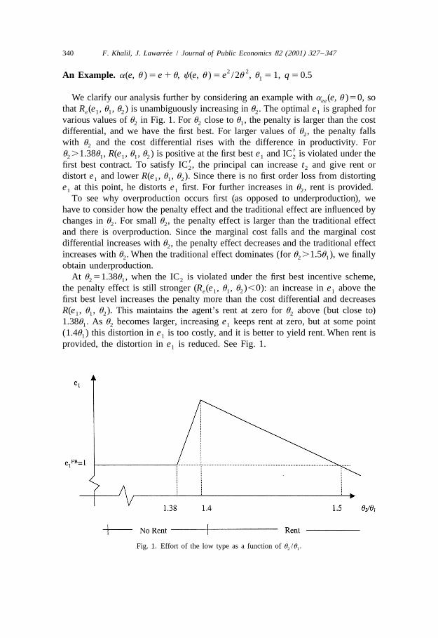
2 2An Example. a(e, u ) 5 e 1u, c(e, u ) 5 e /2u , u 5 1, q 5 0.51

We clarify our analysis further by considering an example with a (e, u )50, soee

that R (e , u , u ) is unambiguously increasing in u . The optimal e is graphed fore 1 1 2 2 1

various values of u in Fig. 1. For u close to u , the penalty is larger than the cost2 2 1

differential, and we have the first best. For larger values of u , the penalty falls2

with u and the cost differential rises with the difference in productivity. For2

9u .1.38u , R(e , u , u ) is positive at the first best e and IC is violated under the2 1 1 1 2 1 2

9first best contract. To satisfy IC , the principal can increase t and give rent or2 2

distort e and lower R(e , u , u ). Since there is no first order loss from distorting1 1 1 2

e at this point, he distorts e first. For further increases in u , rent is provided.1 1 2

To see why overproduction occurs first (as opposed to underproduction), wehave to consider how the penalty effect and the traditional effect are influenced bychanges in u . For small u , the penalty effect is larger than the traditional effect2 2

and there is overproduction. Since the marginal cost falls and the marginal costdifferential increases with u , the penalty effect decreases and the traditional effect2

increases with u . When the traditional effect dominates (for u .1.5u ), we finally2 2 1

obtain underproduction.At u 51.38u , when the IC is violated under the first best incentive scheme,2 1 2

the penalty effect is still stronger (R (e , u , u ),0): an increase in e above thee 1 1 2 1

first best level increases the penalty more than the cost differential and decreasesR(e , u , u ). This maintains the agent’s rent at zero for u above (but close to)1 1 2 2

1.38u . As u becomes larger, increasing e keeps rent at zero, but at some point1 2 1

(1.4u ) this distortion in e is too costly, and it is better to yield rent. When rent is1 1

provided, the distortion in e is reduced. See Fig. 1.1

Fig. 1. Effort of the low type as a function of u /u .2 1


5. Extensions

It is interesting to mention what happens if the principal can impose a fine F .0besides withholding the transfer to the shirking agent. As expected, if F becomesvery large, the principal can secure the first best contract. More importantly, noticethat F affects the penalty (see Proposition 1), but not the penalty effect (seeProposition 2). So as long as the first best is not implementable, the result ofoverproduction survives even if there is an additional penalty F.

Note that if the penalty was transfer independent and only consisted of a fixedfine F, no overproduction would occur in equilibrium. However, a transferdependent penalty, as we have assumed, by itself does not generate

19overproduction . It is the simultaneous presence of ex post choice of monitoringand a transfer dependent penalty that lies behind the result of overproduction inour model.

We can also extend our model to allow the agent to mimic both variables but atsome cost. For instance, when he mimics the input, the agent can also at some costA(.) falsify the output. In our model, A(.) would represent the cost of destroying theextra output (X 2 X ). The other option for the agent, i.e., mimicking the output,2 1

would lead him to falsify the input. This could be achieved by making observedinput unproductive (e.g., employees sitting at the computer but playing solitaire).By analogy we call it the cost of destroying input: B(.).

We model the two functions as A(X 2 X ) and B(X 2 X ). They are assumed to2 1 2 120be increasing and convex with respect to (X 2 X ).2 1

The (IC ) now becomes2

1 ˜(IC )t 2 c(e , u ) $ Maxh0.5[t 2 c(e , u ) 2 c(e , u )]; t 2 c(e , u )2 2 2 2 1 1 2 1 2 1 1 2

˜2 A(.); t 2 c(e , u ) 2 B(.)j1 1 2

The agent has now four options besides telling the truth: he can mimic (i) inputor (ii) output as before; (iii) he can mimic input and falsify output; (iv) he canmimic output and falsify input.

1If A(.) and B(.) are so large that the second and third terms of the RHS of (IC )2

are negative, our model applies unchanged. When it is not the case, overproductioncan still occur. Indeed, the functions A(.) and B(.) can play a role similar to the

19penalty term in (IC ). Therefore the RHS of (IC ) has once again three terms vs.2 2

19Khalil (1997) shows that in a standard auditing model with commitment to auditing, but withtransfer dependent penalty, overproduction does not occur.

20For simplicity we assume that the functions A(.) and B(.) are independent of u. An alternative wayto model mimicking costs can be found in the literature on costly state falsification. (See Crocker and

´Morgan, 1998; Maggi and Rodrıgues-Clare, 1995 and references therein.) However, it wouldcomplicate the analysis by introducing countervailing incentives as in Lewis and Sappington (1989).As long as A(.) and B(.) are not increasing in u, countervailing incentives would not be present.


two in the ex ante model of monitoring. Consider, for example, the situation wherethe agent mimics the input and falsifies the output. The (IC ) is now:2

t 2 c(e , u ) $ t 2 c(e , u ) 2 A(X 2 X )2 2 2 1 1 2 2 1

With (IR ) binding, the rent R is equal to c(e , u ) 2 c(e , u ) 2 A(X 2 X )1 1 1 1 2 2 1

and its derivative with respect to e is R 5c (e , u ) 2 c (e , u ) 2 A9(.)[a (e ,e e 1 1 e 1 2 e 1

u ) 2 a (e , u )]. The objective function can be written as q[a(e , u ) 2 c(e ,2 e 1 1 1 1 1

u )] 1 (1 2 q) [a(e , u ) 2 c(e , u ) 2 R]. According to the first order conditions,1 2 2 2 2FBe 5e and e is such that q[a (e , u ) 2 c (e , u )] 2 (1 2 q)R 50. So if R , 02 2 1 e 1 1 e 1 1 e e

we have overproduction.As before, c (e , u ) 2 c (e , u ) . 0, and once again overproduction can arisee 1 1 e 1 2

because h 2 A9(.)[a (e , u ) 2 a (e , u )]j , 0., i.e., R can be negative. So what ise 1 2 e 1 1 e

crucial to get overproduction is the existence of another term in R (the derivativee

of the rent) that has a negative sign. Ex post monitoring produces this extra termeven when we explicitly model falsification costs.

Whether we continue to obtain the result that the first best is achieved for smallasymmetry of information depends on the properties of the specific falsificationcost function chosen. For instance, if there are fixed costs involved in falsification,the first best will still be reached for small asymmetry of information since thefalsification cost does not disappear as the asymmetry of information reduces.

Therefore, our results generalize to the case where the agent can mimic allvariables. Also, as the number of potential signals increase, so does falsificationcost, and the principal benefits.

6. Conclusions

When multiple screening variables are available, we show that the principal canuse the agent’s fear of getting caught on the wrong foot by choosing themonitoring variable ex post. If the agent’s types are similar (if u /u is small in our2 1

model), this strategy of the principal has strong incentive effects: it yields the firstbest contract. For more serious situations of asymmetry (larger u /u ), the first best2 1

is no longer implementable. We characterize the optimal contract and show that thetraditional result of second best contracting no longer holds. Indeed, the principalmight find it desirable to require the low type to overproduce.

For hidden information problems, our analysis provides a ranking of signals interms of the likelihood of their use as monitoring instruments. Aside from issuesof cost and accuracy, the probability of use is driven by the rent generated. In acontract with ex ante choice of instrument, if the agent can command more rentunder one signal, then that variable will be monitored less often under ex postchoice of instrument. We illustrate this by showing how input monitoring is used


more frequently than output monitoring since there is more rent under outputmonitoring under the ex ante contract.

In real world applications, it may not be possible for the principal to hide forlong the variable to be monitored. This is true, for example, if the chosen variablemust be monitored as soon as the contract takes effect and this cannot be hidden.However, there are many cases where the evaluation takes place once the agent

21has performed his contractual obligations (see the introduction for examples), andour analysis becomes relevant.

In many contractual relationships, the principal has the possibility to observeseveral variables but seems to observe only one of them most of the time. Ourmodel stressed the role of rent, but we need to remember that we have abstractedfrom differences in cost or accuracy between the monitoring instruments. Often, a

22particular monitoring instrument reveals itself as more efficient. The principalshould therefore use that instrument more often. However, our model shows thathaving the opportunity to monitor an alternative variable has important incentiveeffects. If this alternative variable is much less accurate and/or much more costly,the principal should use it with a very small, but positive probability. Also, inreality, different variables have different mimicking costs, which we haveabstracted from. The principal will take these costs into account too whendetermining the frequency of use of monitoring instruments. But our mainmessage will survive, as the principal will benefit from an increase in thedimensionality of the admissible signaling space while monitoring only a subset ofsignals.

Acknowledgements

´We would like to thank Y. Barzel, M. Boyer, N. Bruce, J. Cremer, T. Eicher, M.Ghatak, J. Kline, F. Laux, P. Pestieau, R. Strausz, and M. Van Audenrode forvaluable comments.

Appendix A

A.1. Proof of Lemma 1

* *Replacing (IC ) in the principal’s problem (P), we see that the constraint (IC )2 2

is binding if v [h0, 1j. If v 50, the principal commits to monitor input, and the1 1

high-type’s rent, which is t 2 c(e , u ), equals c(e , u ) 2 c(e , u ).0. By2 2 2 1 1 1 2

21This does not preclude early monitoring as long as the agent is not aware of it.22This could be because it is more accurate and/or less expensive.


*choosing an v slightly positive, the principal can make (IC ) slack and decrease1 2

t . A similar argument can be made for decreasing v from v 51. h2 1 1

A.2. Proof of Proposition 1

9We show that there exists a cut-off u .0, such that if u /u ,u then (IC ) is2 1 2] ]slack under the first best contract and the first best contract is implementable, and

9that if u /u .u then IC is binding and the first best contract is not implement-2 1 2]able.

* 9If R(e , u , u ) is negative, IC is slack under the first best contract. By the1 1 2 2

˜ ˜* * *definition of a(e, u ), e (e , u , u ) is continuous, and lim e (e , u , u ) 5 e .1 1 1 2 u →u 1 1 1 2 12 1

Hence,

* *lim R(e , u , u ) 5 2 c(e , u ) , 0.1 1 2 1 1u →u2 1

Õn the other hand, lim c(e , u ) 5 0 and lim c(e , u ) 5 0. Hence,u →` 1 2 u →` 1 22 2

* *lim R(e , u , u ) 5 c(e , u ) . 0,1 1 2 1 1u →`2

and the first best is no longer implementable for u high enough.2

We complete the proof by showing that R(e , u , u )is monotonically increasing1 1 2

in u :2

ã (e , u )≠R(.) u 1 2˜ ˜]] ]]]5 2 c (e , u ) 1 c (e , u ) 2 c (e , u ) . 0. hF Gu 1 2 e 1 2 u 1 2≠u ã (e , u )2 e 1 2

A.3. Proof of Proposition 2

The Lagrangian is:

L 5 q[a(e , u ) 2 c(e , u )] 1 (1 2 q)[a(e , u ) 2 t ] 2 C1 1 1 1 2 2 2

˜1 l [t 2 c(e , u ) 2 0.5hc(e , u ) 2 c(e , u ) 2 c(e , u )j]1 2 2 2 1 1 1 2 1 2

1 l [t 2 c(e , u )].2 2 2 2

9Consider the case where IC is binding, i.e., l .0. It is easily checked that the2 1

optimal e must satisfy1

a (e , u )e 1 1˜ ]]]q[a (e , u ) 2 c (e , u )] 5 l c (e , u ) 2 c (e , u ) 2 c (e , u ) ,F Ge 1 1 e 1 1 1 e 1 1 e 1 2 e 1 2ã (e , u )e 1 2

; l R (e , u , u ),1 e 1 1 2

where

a (e , u )e 1 1˜ ]]]R (e , u , u ) ; c (e , u ) 2 c (e , u ) 2 c (e , u ).e 1 1 2 e 1 1 e 1 2 e 1 2ã (e , u )e 1 2


If R (e , u , u ) is positive (resp. negative), then under-production (resp. over-e 1 1 2

production) will result. The existence of a solution is demonstrated using anexample in Section 4, and here it is sufficient to show that for u close to u , R (e ,2 1 e 1

u , u ),0 and for large u , R (e , u , u ).0.1 2 2 e 1 1 2

˜lim R (e , u , u ) 5 2 c (e , u ) , 0 since lim e 5 e .u →u e 1 1 2 e 1 1 u →u 1 12 1 2 1

lim R (e , u , u ) 5 c (e , u ) . 0 since lim a (e, u ) 5 `, and limu →` e 1 1 2 e 1 1 u →` e u →`2

c (e, u ) 5 0. he

Ã.4. Conditions for monotonicity of Re(e , u , u )1 1 2

a (e , u )e 1 1]]]≠˜ ˜≠R (e , u , u ) ≠c (e , u ) a (e , u ) a (e , u )e 1 1 2 e 1 2 e 1 1 e 1 2˜]]]] ]]]]]] ]]]]5 2 2 c (e , u )e 1 2≠u ≠u ˜ ≠ua (e , u )2 2 2e 1 2

≠c (e , u )e 1 2]]]2 .

≠u2

˜From the definitions of c(e, u ) and e (e , u , u ), we know that both c (e , u ) and1 1 1 2 e 1 2

e (e , u , u ) are decreasing in u . Therefore, R (e , u , u ) is monotonically1 1 1 2 2 e 1 1 2

˜increasing in u if ≠[a (e , u ) /a (e , u )] /≠u #0. One can check that this occurs2 e 1 1 e 1 2 2

when a (e, u ) is not too large. A sufficient condition is a (e, u )50, while theee ee

necessary condition is

a (e , u )u 1 1˜ ˜ ]]]a (e , u ) 2 a (e , u ) $ 0.eu 1 2 ee 1 2 ã (e , u )e 1 2

References

Anderson, E., Oliver, R.L., 1987. Perspectives on behavior-based versus outcome-based sales forcecontrol systems. Journal of Marketing 51, 76–88.

Baron, D., Besanko, D., 1984. Regulation, asymmetric information, and auditing. RAND Journal ofEconomics 15, 267–302.

Baron, D., Myerson, R., 1982. Regulating a monopolist with unknown cost. Econometrica 50,911–930.

Barzel, Y., 1997. Economic Analysis of Property Rights, 2nd Edition. Cambridge University Press,Cambridge, UK.

Besanko, D., 1994. Performance versus design standards in the regulation of pollution. Journal ofPublic Economics 43, 19–44.

Bontems, P., Bourgeon, J.-M., 2000. Creating countervailing incentives through the choice ofinstruments. Journal of Public Economics 76, 181–202.

Bruce, N., 1998. Public Finance and the American Economy. Addison Wesley.Caillaud, B., Guesnerie, R., Rey, P., Tirole, J., 1988. Government intervention in production and

incentive theory: a review of recent contributions. RAND Journal of Economics 19, 1–26.Chalkley, M., Malcomson, J., 1999. Government purchasing of health services. In: Culyer A

Newhouse, J. (Ed.), Handbook of Health Economics. North Holland.


Ćremer, J., 1995. Arm’s length relationships. Quarterly Journal of Economics 110, 275–295.Crocker, K., Morgan, J., 1998. Is honesty the best policy? Curtailing insurance fraud through optimal

incentive contracts. Journal of Political Economy 106, 355–375.Dewatripont, M., Maskin, E., 1995. Contractual contingencies and renegotiation. Rand Journal of

Economics 26 (4), 704–719.Hart, O., 1995. Firms, Contracts and Financial Structure. Oxford University Press.

¨Holmstrom, B., 1979. Moral hazard and observability. Bell Journal of Economics 10 (1), 74–91.Khalil, F., 1997. Auditing without commitment. Rand Journal of Economics 28 (4), 629–640.

´Khalil, F., Lawarree, J., 1995. Input versus output monitoring: who is the residual claimant? Journal ofEconomic Theory 66 (1), 139–157.

´Kofman, F., Lawarree, J., 1993. Collusion in hierarchical agency. Econometrica 61, 629–656.Laffont, J.-J., Tirole, J., 1993. A Theory of Incentive in Procurement and Regulation. MIT Press.Lafontaine, F., Slade, M., 1996. Retail contracting and costly monitoring: theory and evidence.

European Economic Review 40, 923–932.Lafontaine, F., Slade, M., 1998. Incentive contracting and the franchise decision. Forthcoming in:

Chatterjee, K., Samuelson, W. (Eds), Advances in Business Applications of Game Theory. KluwerAcademic Press, pp. ???-???.

´Lawarree, J., Van Audenrode, M., 1996. Optimal contract, imperfect output observation and limitedliability. Journal of Economic Theory 71 (2), 514–531.

Lewis, T., 1996. Protecting the environment when costs and benefits are privately known. RANDJournal of Economics 27 (4), 819–847.

Lewis, T., Sappington, D., 1989. Countervailing incentives in agency problems. Journal of EconomicTheory 49, 294–313.

Lewis, T., Sappington, D., 1991. Incentives for monitoring quality. RAND Journal of Economics 22(3), 370–384.

Lewis, T., Sappington, D., 1995. Using markets to allocate pollution permits and other scarce resourcesrights under limited information. Journal of Public Economics 57, 431–435.

Maskin, E., Riley, J., 1985. Input versus output based incentive schemes. Journal of Public Economics28, 1–23.

´Maggi, G., Rodrıgues-Clare, A., 1995. Costly distortion of information in agency problems. RANDJournal of Economics 26, 675–689.

´Matutes, C., Regibeau, P., 1994. Compensation schemes and labor market competition: Piece rateversus wage rate. Journal of Economics and Management Strategy 3 (2), 325–353.

Melumad, N., Mookherjee, D., 1989. Delegation as commitment: the case of income tax audits. RANDJournal of Economics 20, 139–163.

Mirrlees, J., 1971. An exploration in the theory of optimum income taxation. Review of EconomicStudies 38 (114), 175–208.

Mookherjee, D., Png, I., 1989. Optimal auditing, insurance and redistribution. Quarterly Journal ofEconomics CIV, 399–416.

New York Times, 2000, June 16. Asleep at the Books: A Fraud that went On and On and On. SectionC, page 1.

Rochet, J.-C., Stole, L., 2000. The economics of multidimensional screening. Working paper Universityof Chicago.

Sappington, D., 1983. Optimal regulation of a multiproduct monopoly with unknown technologicalcapabilities. Bell Journal of Economics 14, 453–463.

Schmutzler, A., Goulder, L., 1997. The choice between emission taxes and output taxes underimperfect monitoring. Journal of Environmental Economics and Management 32 (1), 51–64.

Singh, N., 1989. Theories of sharecropping. In: Bardhan, P. (Ed.), The Economic Theory of AgrarianInstitutions. Clarendon, Oxford.

Strausz, R., 1997. Delegation of monitoring in a principal-agent relationship. Review of EconomicStudies 64 (3), 337–357.


Swierzbinski, J., 1994. Guilty until proven innocent-regulation with costly and limited enforcement.Journal of Environmental Economics and Management 27 (2), 127–146.

Wittman, D., 1977. Prior regulation versus post liability: The choice between input and outputmonitoring. Journal of Legal Studies VI (1), 193–211.

Documents

Catching the agent on the wrong foot: ex post choice of monitoring