Embed Size (px)
Citation preview
Causal Discovery for Manufacturing Domains
Katerina MarazopoulouCollege of Information and
Computer SciencesUMass Amherst
Rumi GhoshData Mining Services and
Solutions, Robert Bosch LLCPalo Alto, USA
Prasanth LadeData Mining Services and
Solutions, Robert Bosch LLCPalo Alto, USA
[email protected] Jensen
College of Information andComputer Sciences
UMass [email protected]
ABSTRACTIncreasing yield and improving quality are of paramount im-portance to any manufacturing company. One of the ways toachieve this is through discovery of the causal factors that af-fect these quantities. In this work, we use data-driven causalmodels to identify causal relationships in manufacturing.Specifically, we apply causal structure learning techniqueson real data collected from a production line. Emphasis isgiven to the interpretability of the learned causal models, sothat they can be used by practitioners to take meaningfulactions. We highlight the challenges presented by assembly-line data and propose ways to address those challenges. Wealso identify unique characteristics of data originating fromassembly lines and how to leverage those characteristics toimprove causal discovery. Standard evaluation techniquesfor causal structure learning show that the learned modelsclosely match the underlying causal relationships betweendifferent factors in the production process. These resultswere also validated by manufacturing domain experts, whofound them promising. This work demonstrates how datamining and knowledge discovery can be used for root causeanalysis in the domain of manufacturing and connected in-dustry.
Categories and Subject DescriptorsH.2.8 [Database Management]: Database Applications—Data mining ; I.2.6 [Artificial Intelligence]: Learning—Concept learning, knowledge acquisition; J.1 [ComputerApplications]: Administrative Data Processing—Manufac-turing
KeywordsCausal Discovery, Manufacturing, Structure Learning
Permission to make digital or hard copies of all or part of this work forpersonal or classroom use is granted without fee provided that copies arenot made or distributed for profit or commercial advantage and that copiesbear this notice and the full citation on the first page. To copy otherwise, torepublish, to post on servers or to redistribute to lists, requires prior specificpermission and/or a fee.Copyright 20XX ACM X-XXXXX-XX-X/XX/XX ...$15.00.
1. INTRODUCTIONWith increasing interest in the Internet of Things (IoT),
the size and complexity of data sets collected from manufac-turing processes has grown significantly. The ability to usenetworked devices and sensors in assembly lines has enabledcollection of data from every stage of the manufacturing pro-cess. However, the collection of arbitrarily large amounts ofdata is meaningful only if it leads to actionable insights, es-pecially on how to increase yield and efficiency. Our work isa step in this direction.
This work has two objectives. First, we aim to identifythe joint causal structure of a specific manufacturing do-main. Second, we focus on the the key causal factors thatincrease yield. To be more specific, given the measurementstaken during the production and testing of a product, weaim to identify the causal relationships of the domain, whichinclude the influential factors affecting yield.
The traditional approach to address this issue is throughDesign of Experiments (DoE) [3]. In the context of man-ufacturing, DoE usually includes carrying out experimentsin the real production and testing environment. As a con-sequence, it can be costly and time-consuming. Therefore,practitioners limit the number of factors examined in eachexperiment. As the process of manufacturing becomes morecomplex, sometimes comprising hundreds of possible factors,it becomes very difficult to choose the appropriate factors forfurther investigation through DoE. Currently, most expertsin manufacturing rely on domain knowledge and intuitionalong with basic statistics to guide their efforts to increaseyield and improve quality.
This work aims to aid this process by using data miningand knowledge discovery. Specifically, we apply techniquesfor learning causal structure from real data collected froma manufacturing line in order to identify the key factorsaffecting yield and the complex interrelationships amongstthem1.
Algorithms for learning causal structure construct a causalgraphical model over the variables of a domain. Such mod-els aim to identify the underlying causal mechanisms of aspecific domain. Causal models are of great value, becauseknowing the causes of a target variable specifies interven-
1Efforts are ongoing to make this data set public for thebenefit of the knowledge discovery and data mining commu-nities.
arX
iv:1
605.
0405
6v2
[cs
.LG
] 1
3 Ju
n 20
16
tions on other variables that can change the target variablein a desired way. Causal models have been applied in areassuch as planning, decision making, epidemiology, and socialscience, just to mention a few.
In what follows, we first describe the manufacturing do-main, i.e., the manufacturing process and the structure ofan assembly line. We then provide a short introduction tographical models and causal discovery algorithms. We showqualitative results obtained from application of causal dis-covery algorithms on the data collected from a productionline. We identify the specific challenges presented by manu-facturing data and how the standard algorithms need to bemodified in order to improve causal discovery. Finally, wepresent an evaluation of causal structure learning for man-ufacturing, based on domain expertise and synthetic data.
2. THE MANUFACTURING DOMAINTypical assembly lines consist of multiple stations where
different operations take place. In every station, severalmeasurements are taken for the product up to that point.Components are added to an unfinished product in differentproduction stations of an assembly line. A testing station isa station where a product passing through is inspected. Ad-ditionally, at the end of the assembly line, there are usuallytesting stations—called end-of-line (EOL) testing stations—which inspect the final product. Testing stations carry outa series of measurements to test the quality of the product.If the product does not meet the required quality criteria, itis usually rejected. A rejected product is called a scrap andan accepted product is called a good part.
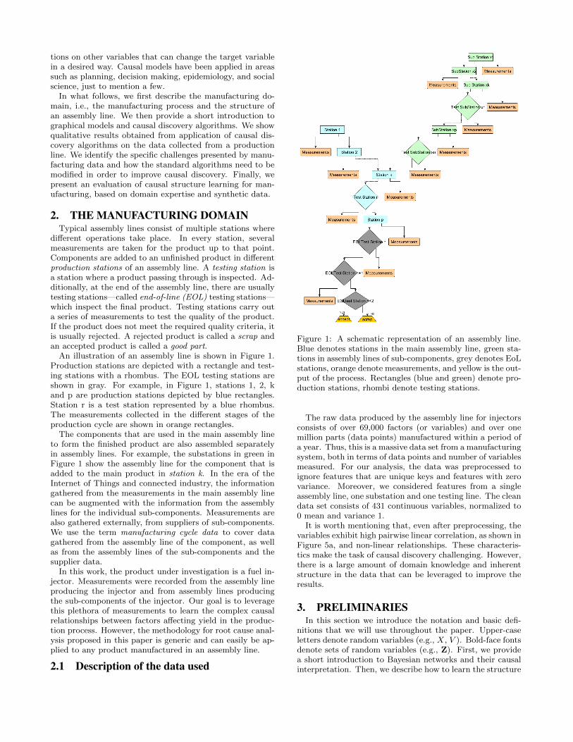
An illustration of an assembly line is shown in Figure 1.Production stations are depicted with a rectangle and test-ing stations with a rhombus. The EOL testing stations areshown in gray. For example, in Figure 1, stations 1, 2, kand p are production stations depicted by blue rectangles.Station r is a test station represented by a blue rhombus.The measurements collected in the different stages of theproduction cycle are shown in orange rectangles.
The components that are used in the main assembly lineto form the finished product are also assembled separatelyin assembly lines. For example, the substations in green inFigure 1 show the assembly line for the component that isadded to the main product in station k. In the era of theInternet of Things and connected industry, the informationgathered from the measurements in the main assembly linecan be augmented with the information from the assemblylines for the individual sub-components. Measurements arealso gathered externally, from suppliers of sub-components.We use the term manufacturing cycle data to cover datagathered from the assembly line of the component, as wellas from the assembly lines of the sub-components and thesupplier data.
In this work, the product under investigation is a fuel in-jector. Measurements were recorded from the assembly lineproducing the injector and from assembly lines producingthe sub-components of the injector. Our goal is to leveragethis plethora of measurements to learn the complex causalrelationships between factors affecting yield in the produc-tion process. However, the methodology for root cause anal-ysis proposed in this paper is generic and can easily be ap-plied to any product manufactured in an assembly line.
2.1 Description of the data used
Figure 1: A schematic representation of an assembly line.Blue denotes stations in the main assembly line, green sta-tions in assembly lines of sub-components, grey denotes EoLstations, orange denote measurements, and yellow is the out-put of the process. Rectangles (blue and green) denote pro-duction stations, rhombi denote testing stations.
The raw data produced by the assembly line for injectorsconsists of over 69,000 factors (or variables) and over onemillion parts (data points) manufactured within a period ofa year. Thus, this is a massive data set from a manufacturingsystem, both in terms of data points and number of variablesmeasured. For our analysis, the data was preprocessed toignore features that are unique keys and features with zerovariance. Moreover, we considered features from a singleassembly line, one substation and one testing line. The cleandata set consists of 431 continuous variables, normalized to0 mean and variance 1.
It is worth mentioning that, even after preprocessing, thevariables exhibit high pairwise linear correlation, as shown inFigure 5a, and non-linear relationships. These characteris-tics make the task of causal discovery challenging. However,there is a large amount of domain knowledge and inherentstructure in the data that can be leveraged to improve theresults.
3. PRELIMINARIESIn this section we introduce the notation and basic defi-
nitions that we will use throughout the paper. Upper-caseletters denote random variables (e.g., X, V ). Bold-face fontsdenote sets of random variables (e.g., Z). First, we providea short introduction to Bayesian networks and their causalinterpretation. Then, we describe how to learn the structure
of such models from data.
3.1 Bayesian NetworksBayesian networks are directed graphical models that com-
pactly represent sets of probability distributions. A Bayesiannetwork defined over a set of random variables V consistsof:
1. A directed acyclic graph G = 〈V,E〉, known as thestructure of the network, and
2. A set of parameters Θ, where every parameter θ ∈ Θis a conditional distribution of a node given its parentsin the graph.
A graph G is a partially directed graph if it has both di-rected and undirected edges. The skeleton of a graph G isthe undirected graph that can be obtained by substitutingevery edge of G with an undirected edge. A path betweentwo nodes X and Y is a sequence of nodes X,V1, . . . , Vn, Ysuch that there exists an edge between every two consecutivenodes of the path. A v-structure or collider on a graph G isan ordered triple of nodes 〈X,Y, Z〉 such that X → Y ← Zand there is no edge between X and Z.
The structure of a Bayesian network represents a set ofindependencies according to the local Markov condition: anode is independent of its non-descendants given its parentsin the graph. The same set of independencies can be derivedthrough the use of the graphical criterion of d-separation.We say that two nodes V1 and V2 are d-separated given adisjoint set of variables Z if there are no d-connecting pathsbetween V1 and V2 given Z. A path between V1 and V2
is d-connecting given a set Z, if every collider along thepath is in Z or has a descendant in Z and no other nodesare in Z. It is worth noting that different directed acyclicgraphs might represent the same set of independencies. Thatset of DAGs is known as the Markov equivalence class forthat set of independencies. A Markov equivalence class canbe graphically represented by a mixed graph (a graph thatcontains both directed and undirected edges). For everyundirected edge, any of the two possible orientations doesnot change the set of conditional independencies induced bythe graph.
3.2 Causal Bayesian NetworksThe notion of causality has been a subject of debate for
philosophers and practitioners since ancient times. In thiswork, we focus on the semantics of causality based on prob-abilistic distributions and manipulations, following the workof Pearl [11] and Spirtes et al. [18]. In this framework, Xis a direct cause of Y with respect to a set of variables Z ifchanging the value of X results in changes in the probabil-ity distribution of Y , assuming that the values of all othervariables in Z are held constant [17].
To interpret graphs (and thus Bayesian networks) causallyand use them for causal inference and discovery, we need tomake an additional set of assumptions.
1. Causal Sufficiency: There are no unmeasured commoncauses of a measured variable.
2. Causal Markov condition: The Markov condition andd-separation provide a connection between the struc-ture of a Bayesian network and the independenciesthat hold in the underlying distribution. If we want to
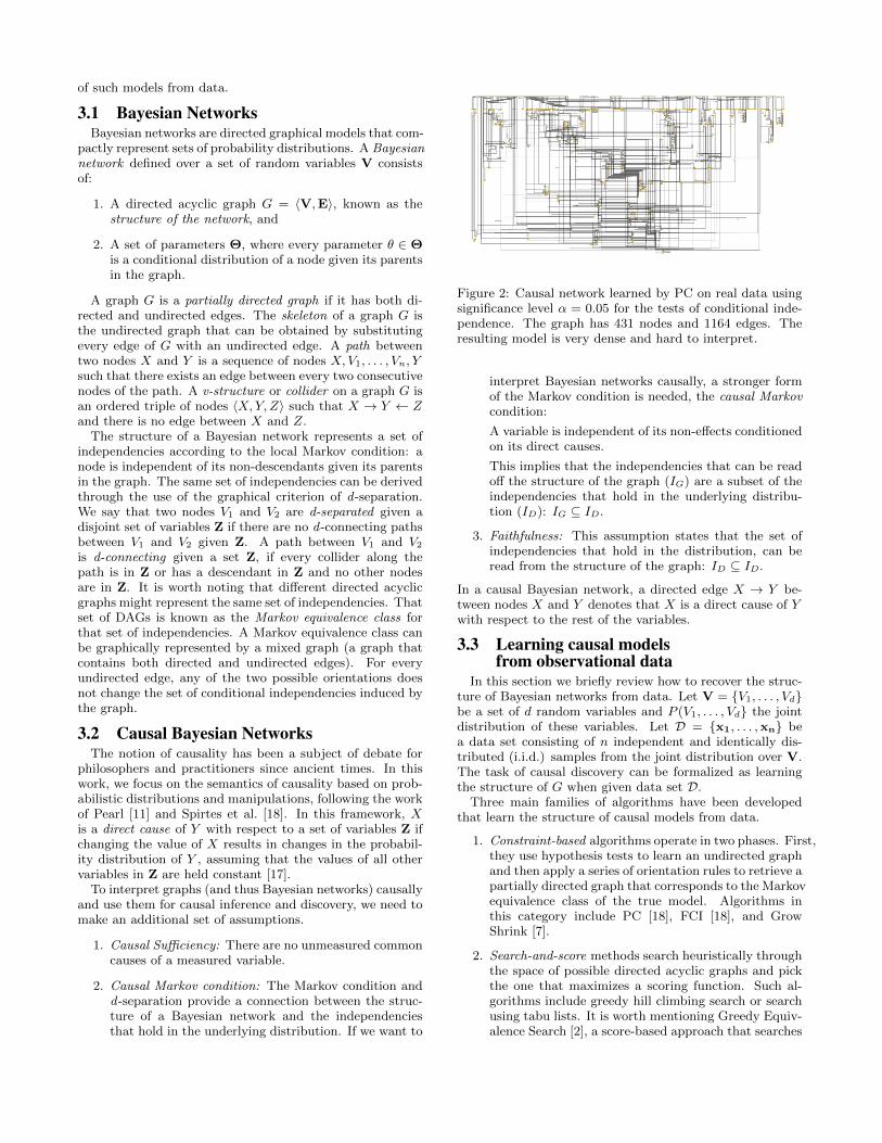
Figure 2: Causal network learned by PC on real data usingsignificance level α = 0.05 for the tests of conditional inde-pendence. The graph has 431 nodes and 1164 edges. Theresulting model is very dense and hard to interpret.
interpret Bayesian networks causally, a stronger formof the Markov condition is needed, the causal Markovcondition:
A variable is independent of its non-effects conditionedon its direct causes.
This implies that the independencies that can be readoff the structure of the graph (IG) are a subset of theindependencies that hold in the underlying distribu-tion (ID): IG ⊆ ID.
3. Faithfulness: This assumption states that the set ofindependencies that hold in the distribution, can beread from the structure of the graph: ID ⊆ ID.
In a causal Bayesian network, a directed edge X → Y be-tween nodes X and Y denotes that X is a direct cause of Ywith respect to the rest of the variables.
3.3 Learning causal modelsfrom observational data
In this section we briefly review how to recover the struc-ture of Bayesian networks from data. Let V = {V1, . . . , Vd}be a set of d random variables and P (V1, . . . , Vd} the jointdistribution of these variables. Let D = {x1, . . . ,xn} bea data set consisting of n independent and identically dis-tributed (i.i.d.) samples from the joint distribution over V.The task of causal discovery can be formalized as learningthe structure of G when given data set D.
Three main families of algorithms have been developedthat learn the structure of causal models from data.
1. Constraint-based algorithms operate in two phases. First,they use hypothesis tests to learn an undirected graphand then apply a series of orientation rules to retrieve apartially directed graph that corresponds to the Markovequivalence class of the true model. Algorithms inthis category include PC [18], FCI [18], and GrowShrink [7].
2. Search-and-score methods search heuristically throughthe space of possible directed acyclic graphs and pickthe one that maximizes a scoring function. Such al-gorithms include greedy hill climbing search or searchusing tabu lists. It is worth mentioning Greedy Equiv-alence Search [2], a score-based approach that searches
X Y
Z
X Y
ZZ 62 SeparatingSet(X, Y )
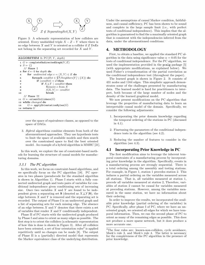
Figure 3: A schematic representation of how colliders areoriented. Every unshielded triple X −Z − Y where there isno edge between X and Y is oriented as a collider if Z DoEsnot belong in the separating set recorded for X and Y .
ALGORITHM 1: PC(D, V , depth)
1 G← completeUndirectedGraph(V,E)2 S ← {}
// Phase I3 for d← 0 to depth do4 for undirected edge e = 〈X,Y 〉 ∈ E do
5 foreach condSet ∈℘(Neighbors[Y ] \ {X}) do6 if |condSet | = d then7 if X |= Y | condSet then8 Remove e from E9 S[X,Y ]← condSet
10 break
// Phase II11 G← orientColliders(G)12 while changed do13 G← applyOrientationRyles(G)14 return G
over the space of equivalence classes, as opposed to thespace of DAGs.
3. Hybrid algorithms combine elements from both of theaforementioned approaches. They use hypothesis teststo limit the space of available models and then searchover the constrained space to find the best orientedmodel. An example of a hybrid algorithm is MMHC [21].
In this work, we explore the use of constraint-based meth-ods for learning the structure of causal models for manufac-turing domains.
3.3.1 The PC algorithmIn this work, we focus on constraint-based algorithms, and
we specifically focus on the PC algorithm [18]. PC oper-ates in two phases (pseudocode for the standard algorithmis shown in Algorithm 1). Phase I starts with a fully con-nected undirected graph and tests pairs of variables for con-ditional independence given conditioning sets of increasingsize. Once two variables X and Y are found to be inde-pendent given a separating set S (denoted as X |= Y |S), theedge between X and Y is removed and the separating set isrecorded. The output of Phase I is an undirected graph anda list of separating sets for each missing edge. The absenceof an edge between X and Y denotes that there exists a setof variables that render X and Y conditionally independent.
Phase II of PC starts with the undirected graph producedby Phase I and aims to orient as many edges as possible. Thefirst step is to orient the colliders (a schematic representationof how this is done is shown in Figure 3). After all collidershave been oriented, a set of four orientation rules2 is appliedrepetitively until no changes can be made [8]. The outputof Phase II is a (partially) directed model that representsthe Markov equivalence class of the underlying distribution.
Under the assumptions of causal Markov condition, faithful-ness, and causal sufficiency, PC has been shown to be soundand complete in the large sample limit (i.e., with perfecttests of conditional independence). This implies that the al-gorithm is guaranteed to find the a maximally oriented graphthat is consistent with the independencies inferred from thedata, under the aforementioned conditions.
4. METHODOLOGYFirst, to obtain a baseline, we applied the standard PC al-
gorithm in the data using significance value α = 0.05 for thetests of conditional independence. For the PC algorithm, weused the implementation provided in the pcalg package [5](with appropriate modifications, as explained below). Weused Fisher’s z-transformation of the partial correlation asthe conditional independence test (throughout the paper).
The learned graph is shown in Figure 2. It consists of431 nodes and 1164 edges. This simplistic approach demon-strates some of the challenges presented by manufacturingdata. The learned model is hard for practitioners to inter-pret, both because of the large number of nodes and thedensity of the learned graphical model.
We now present modifications on the PC algorithm thatleverage the properties of manufacturing data to learn aninterpretable causal model of the domain. Specifically, weconsider the following adjustments:
1. Incorporating the prior domain knowledge regardingthe temporal ordering of the stations in PC (discussedin 4.1).
2. Finetuning the parameters of the conditional indepen-dence tests in the algorithm (see 4.2).
3. Reducing the number of features to consider in thealgorithm (see 4.3).
4.1 Incorporating Prior Knowledge in PCThe first modification aims to leverage the inherent tem-
poral constraints of a manufacturing process by incorporat-ing prior knowledge in the algorithm. Specifically, events ina manufacturing process are strongly sequential. There isa total ordering among the assembly and testing stations.For example, in Figure 1, station 1 precedes station 2. Thisinduces a partial ordering on the variables measured acrossall stations. That is, all variables measured at station 1,precede all variables measured at station 2, Therefore, vari-ables of station 2 cannot be causal for variables measuredat preceding stations. However, among the variables mea-sured in the same station, we have no information abouttheir ordering.
In order to improve the results, we incorporated the avail-able prior knowledge (partial ordering of the variables) inPC. Specifically, after phase I of PC, where we have an un-oriented graph, we oriented all edges for which we have tem-poral information. Then, we ran the second phase of PC toorient as many of the remaining edges as possible. This doesnot produce a more sparse network, but it does produce amore accurate one.
2The four rules are: known-non-colliders, cycle avoidance,Meek’s rule 3, and Meek’s rule 4. The latter is necessaryfor the completeness of the PC algorithm in the presence ofprior knowledge.
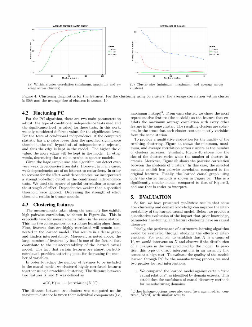
(a) Within cluster correlation (minimum, maximum and av-erage across clusters).
(b) Cluster size (minimum, maximum, and average acrossclusters).
Figure 4: Clustering diagnostics for the features. For the clustering using 50 clusters, the average correlation within clusteris 80% and the average size of clusters is around 10.
4.2 Finetuning PCFor the PC algorithm, there are two main parameters to
adjust: the type of conditional independence tests used andthe significance level (α value) for these tests. In this work,we only considered different values for the significance level.For the tests of conditional independence, if the computedstatistic has a p-value lower than the specified significancethreshold, the null hypothesis of independence is rejected,and thus the edge is kept in the model. The higher the αvalue, the more edges will be kept in the model. In otherwords, decreasing the α value results in sparser models.
Given the large sample size, the algorithm can detect evenvery weak dependencies from data. However, in many cases,weak dependencies are of no interest to researchers. In orderto account for the effect weak dependencies, we incorporateda strength-of-effect cutoff in the conditional independencetests. We used the square of partial correlation to measurethe strength of effect. Dependencies weaker than a specifiedthreshold were ignored. Decreasing the strength of effectthreshold results in denser models.
4.3 Clustering featuresThe measurements taken along the assembly line exhibit
high pairwise correlation, as shown in Figure 5a. This isespecially true for measurements taken in the same station.This has two consequences for structure learning algorithms.First, features that are highly correlated will remain con-nected in the learned model. This results in a dense graphand hinders interpretability. Moreover, as noted above, thelarge number of features by itself is one of the factors thatcontribute to the uninterpretability of the learned causalmodel. The fact that certain features are almost perfectlycorrelated, provides a starting point for decreasing the num-ber of variables.
In order to reduce the number of features to be includedin the causal model, we clustered highly correlated featurestogether using hierarchical clustering. The distance betweentwo features X and Y was defined as
d(X,Y ) = 1− |correlation(X,Y )|.
The distance between two clusters was computed as themaximum distance between their individual components (i.e.,
maximum linkage)3. From each cluster, we chose the mostrepresentative feature (the medoid) as the feature that ex-hibits the maximum average correlation with every otherfeature in the same cluster. The resulting clusters are coher-ent, in the sense that each cluster contains mostly variablesfrom the same station.
To provide a qualitative evaluation for the quality of theresulting clustering, Figure 4a shows the minimum, maxi-mum, and average correlation across clusters as the numberof clusters increases. Similarly, Figure 4b shows how thesize of the clusters varies when the number of clusters in-creases. Moreover, Figure 5b shows the pairwise correlationbetween the medoids of clusters. In this case, the selectedmedoids exhibit less pairwise correlation compared to theoriginal features. Finally, the learned causal graph usingonly the cluster medoids is shown in Figure 6a. This is asignificantly smaller model, compared to that of Figure 2,and one that is easier to interpret.
5. EVALUATIONSo far, we have presented qualitative results that show
how clustering and domain knowledge can improve the inter-pretability of the learned causal model. Below, we provide aquantitative evaluation of the impact that prior knowledge,parameter fine-tuning, and feature clustering have on causaldiscovery.
Ideally, the performance of a structure-learning algorithmwould be evaluated through studying the effects of inter-ventions. For example, to establish that X is a cause ofY , we would intervene on X and observe if the distributionof Y changes in the way predicted by the model. In prac-tice, this type of direct interventions in an assembly linecomes at a high cost. To evaluate the quality of the modelslearned through PC for the manufacturing process, we usedtwo proxies for real interventions:
1. We compared the learned model against certain “truecausal relations”, as identified by domain experts. Thisestablishes the usefulness of causal discovery methodsfor manufacturing domains.
3Other linkage options were also used (average, median, cen-troid, Ward) with similar results.

(a) Pairwise correlation between the original features. (b) Pairwise correlation between the medoids of theclusters.
Figure 5: Pairwise correlation between features before (left) and after (right) applying hierarchical clustering.
2. In order to evaluate different variants of the PC al-gorithm, we used synthetic models to generate datasimilar to the real data produced by the manufactur-ing line. We then compared the accuracy of modelslearned through different variants of PC against thegenerative model.
5.1 Evaluation through domain expertiseOne way to partially evaluate the effectiveness of causal
structure learning in this manufacturing domain is throughthe use of domain knowledge. As noted earlier, Figure 6acontains causal relationships extracted by our model on areduced feature set. Domain experts also provided partialground truth where they identified nine critical features thatare causal for the target variable of interest, based on theirexpertise and knowledge of the physical properties of themanufacturing line. We indexed each of these features usingthe medoids of the clusters from the hierarchical clusteringthat they belonged to. We found that these nine featuresbelonged to three clusters with medoids F32, F25 and F9.From Figure 6a, we observe that F32, F25 and F9 indeedare identified as causes of the target variable F37. Figure 6bcontains the exact paths extracted from the full causal modelthat contain these critical features. This confirms that thecausal structure learned from the data agrees with the causalpaths provided by the domain experts.
5.2 Evaluation through the use ofsynthetic models
The fact that the learned causal model matches the intu-ition and knowledge of domain experts is very encouraging.However, it only provides validation for a small part of themodel (the nine features identified as causes for the targetvariable). Unfortunately, the lack of ground truth makes theevaluation of the complete causal model impossible (at leastwithout performing experiments directly on the productionline). To quantify the performance of causal discovery tech-niques in the manufacturing domain given the absence ofground truth, we turn to synthetic models and simulateddata. Specifically, we use a synthetic model to generate data
and we treat the generating model as the ground truth. Ide-ally, the synthetic model will be similar to the actual modelthat describes the domain, and the generated data will re-semble the real data produced by an assembly line.
5.2.1 Generation of synthetic dataThe first step towards the evaluation through synthetic
data is the generation of the synthetic model and data. Theprocedure we followed is outlined below:
• We used a data set Doriginal containing data producedby an actual production line to learn a causal modelMtrue ec using the PC algorithm with parameters α =0.05 and strength of effect equal to 0.01. Note that weused the available temporal information when learn-ing Mtrue eq . Mtrue eq represents a Markov equiva-lence class and thus, contains both directed and undi-rected edges. To generate data, we need a fully di-rected model. Therefore, we randomly picked a mem-ber of the Markov equivalence class Mgenerating . Thisis a fully directed model that, by definition, respectsthe orientations enforced by the prior knowledge.
• We then learned parameters for Mgenerating using theoriginal data set Doriginal . The parametric form of theconditional distributions was assumed to be Gaussian.
• We used the learned modelMgenerating with the learnedparameters to generate a set of 10 synthetic data sets,Di
synthetic , i = {1, . . . , 10} with 50000 data points each4.
• Finally, we ran the PC algorithm on the synthetic datausing varying values for the significance level and thestrength of effect:
α = {0.001, 0.01, 0.05, 0.1}soe = {0, 0.05, 0.1}
4To learn the parameters of the Bayesian network and gen-erate data from the model, we used the bnlearn package forR [14].
(a) Causal model learned by PC using only the medoids of the 50clusters created with hierarchical clustering. The green node is thecluster that corresponds to the target variable (yield). Note that thefeature names have been anonymized.
(b) The paths containing critical features provided by the Domainexperts (in red).
Figure 6: Application of PC on the clustered features onreal data.
The process we followed to generate synthetic data as-sumes that the features follow a Gaussian distribution. Weevaluated this assumption by calculating the skewness andkurtosis for each feature distribution. Out of the 50 medoidswe have extracted, we observed 26 features to have skew-ness and kurtosis values within the range of -2 to +2. Thisempirically indicates that 52% of the features are within anacceptable range that indicates normality. We compared thedistribution of the generated features to that of the actualfeatures, in order to demonstrate that the synthetic datawe produce resemble the real data. Figure 7 depicts thedistribution of the actual feature compared to that of thegenerated features for three features.
5.2.2 Results on synthetic dataTo evaluate the performance of PC on synthetic data we
used precision and recall after Phase I (undirected model)and after Phase II (partially directed model).
UndirectedPrecision =# of true learned edges
# of learned edges
UndirectedRecall =# of true learned edges
# of true edges
DirectedPrecision =# of true learned oriented edges
# of learned oriented edges
DirectedRecall =# of true learned oriented edges
# of true oriented edges
Actual Synthetic
(a) Example features where the actual data follows anormal distribution.
Actual Synthetic
(b) Example feature where the actual data follows anon-normal distribution.
Figure 7: Comparison between the density of actual featuresand their synthetically generated counterparts.
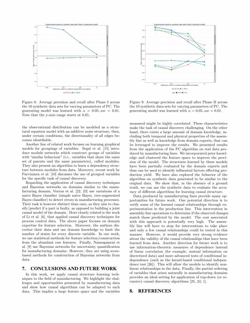
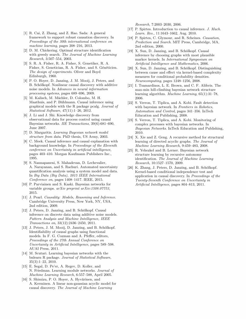
The average precision and recall values across the 10 syn-thetic data sets after Phase I are shown in Figure 8. Thealgorithm has almost perfect recall (it learns all the trueedges). The precision of the algorithm drops as the signif-icance level of the test increases. This is to be expected,because higher α values result in a denser graph, therefore,more edges will be incorrectly included in the output. Theresults after Phase II are presented in Figure 9. As the al-pha values increases, the recall increases and the algorithmretrieves more than 50% of the true directions. However,the precision drops, suggesting that it is making more mis-takes in the orientations. This can be explained because thelearned model includes more spurious (directed) edges.
6. RELATED WORKIn the area of causal discovery, the constraint-based al-
gorithms we focused on retrieve models up to the Markovequivalence class (and thus might contain undirected edges).The authors of [20, 19] describe principled ways to choose aspecific model from the Markov equivalence class. Moreover,apart from the structure learning algorithms that leverageconditional independence, there exist other techniques to re-trieve causal relationships from observational data. In thepast few years, a group of methods based on additive noisemodels (ANMs) has been proposed [16, 4, 13, 12]. ANMsleverage properties of the joint distribution other than con-ditional independence. In short, it has been shown that if
●●●
●●●
●●●
●●●
●●● ●●● ●●● ●●●
0.7
0.8
0.9
1.0
0.7
0.8
0.9
1.0
precision.undirectedrecall.undirected
0.001 0.01 0.05 0.1Significance value for conditional independence test (alpha).
Val
ue o
f met
ric (
prec
isio
n or
rec
all)
soe ● ● ●0.001 0.01 NA
Experimental results on synthetic data after Phase I (undirected model)
Figure 8: Average precision and recall after Phase I acrossthe 10 synthetic data sets for varying parameters of PC. Thegenerating model was learned with α = 0.05, soe = 0.01.Note that the y-axis range starts at 0.65.
the observational distribution can be modeled as a struc-tural equation model with an additive noise structure, then,under certain conditions, the directionality of all edges be-comes identifiable.
Another line of related work focuses on learning graphicalmodels for groupings of variables. Segal et al. [15] intro-duce module networks which construct groups of variableswith “similar behaviour” (i.e., variables that share the sameset of parents and the same parameters), called modules.They also present an algorithm to learn a dependency struc-ture between modules from data. Moreover, recent work byParviainen et al. [10] discusses the use of grouped variablesfor the specific task of causal discovery.
Regarding the application of causal discovery techniquesand Bayesian networks on domains similar to the manu-facturing domain, Verron et al. [22, 23] use variations of anaive Bayes classifier (simple naive Bayes, tree-augmentedBayes classifier) to detect errors in manufacturing processes.Their task is however distinct than ours, as they aim to clas-sify/predict if a part is faulty, as opposed to building a jointcausal model of the domain. More closely related is the workof Li et al. [6], that applied causal discovery techniques forprocess control data. The above paper focuses on domainexpertise for feature selection. Moreover, the authors dis-cretize their data and use domain knowledge to limit thenumber of states for every discrete variable. In our work,we use statistical methods for feature selection/constructionfrom the abundant raw features. Finally, Nannapaneni etal. [9] use Bayesian networks for uncertainty quantificationfor manufacturing domains. However, they are using score-based methods for construction of Bayesian networks fromdata.
7. CONCLUSIONS AND FUTURE WORKIn this work, we apply causal structure learning tech-
niques to the field of manufacturing. We highlight the chal-lenges and opportunities presented by manufacturing dataand show how causal algorithms can be adapted to suchdata. This implies a large feature space and the variables
●
●
●
●
●●
●
●
●
●
●
●
●●●
●●
●
●
●●
●
●
●
0.35
0.40
0.45
0.50
0.35
0.40
0.45
0.50
precision.directedrecall.directed
0.001 0.01 0.05 0.1Significance value for conditional independence test (alpha).
Val
ue o
f met
ric (
prec
isio
n or
rec
all)
soe ● ● ●0.05 0.1 NA
prior ● FALSE TRUE
Experimental results on synthetic data after Phase II (directed model)
Figure 9: Average precision and recall after Phase II acrossthe 10 synthetic data sets for varying parameters of PC. Thegenerating model was learned with α = 0.05, soe = 0.01.
measured might be highly correlated. These characteristicsmake the task of causal discovery challenging. On the otherhand, there exists a large amount of domain knowledge, in-cluding both temporal and physical properties of the assem-bly line as well as knowledge from domain experts, that canbe leveraged to improve the results. We presented resultsfrom the application of the PC algorithm on real data pro-duced by manufacturing lines. We incorporated prior knowl-edge and clustered the feature space to improve the preci-sion of the model. The structures learned by these modelshave been partially evaluated by the domain experts andthus can be used to identify influential factors effecting pro-duction yield. We have also explored the behavior of thealgorithm on synthetic data generated to be similar to theoriginal data. We show that, in the absence of a groundtruth, we can use the synthetic data to evaluate the accu-racy of different algorithms for learning causal structure.
Data produced by manufacturing lines provide many op-portunities for future work. One potential direction is toverify some of the learned causal relationships through ex-perimentation in the production line. This intervention inassembly-line operations to determine if the observed changesmatch those predicted by the model. The cost associatedwith this approach is potentially very high. The assem-bly line will have to stop for interventions to take placeand only a few causal relationships could be tested in thismanner. However, it would provide very strong evidenceabout the validity of the causal relationships that have beenlearned from data. Another direction for future work is touse information-theoretic measures of dependence insteadof linear correlation (for example, mutual information ondiscretized data) and more advanced tests of conditional in-dependence (such as the kernel-based conditional indepen-dence test [26]). This will allow the models to identify non-linear relationships in the data. Finally, the partial orderingof variables that arises naturally in manufacturing domainsprovides an ideal setting for application of top-down (or re-cursive) causal discovery algorithms [25, 24, 1].
8. REFERENCES
[1] R. Cai, Z. Zhang, and Z. Hao. Sada: A generalframework to support robust causation discovery. InProceedings of the 30th international conference onmachine learning, pages 208–216, 2013.
[2] D. M. Chickering. Optimal structure identificationwith greedy search. The Journal of Machine LearningResearch, 3:507–554, 2003.
[3] S. R. A. Fisher, R. A. Fisher, S. Genetiker, R. A.Fisher, S. Genetician, R. A. Fisher, and S. Geneticien.The design of experiments. Oliver and BoydEdinburgh, 1960.
[4] P. O. Hoyer, D. Janzing, J. M. Mooij, J. Peters, andB. Scholkopf. Nonlinear causal discovery with additivenoise models. In Advances in neural informationprocessing systems, pages 689–696, 2009.
[5] M. Kalisch, M. Machler, D. Colombo, M. H.Maathuis, and P. Buhlmann. Causal inference usinggraphical models with the R package pcalg. Journal ofStatistical Software, 47(11):1–26, 2012.
[6] J. Li and J. Shi. Knowledge discovery fromobservational data for process control using causalBayesian networks. IIE Transactions, 39(6):681–690,June 2007.
[7] D. Margaritis. Learning Bayesian network modelstructure from data. PhD thesis, US Army, 2003.
[8] C. Meek. Causal inference and causal explanation withbackground knowledge. In Proceedings of the Eleventhconference on Uncertainty in artificial intelligence,pages 403–410. Morgan Kaufmann Publishers Inc.,1995.
[9] S. Nannapaneni, S. Mahadevan, D. Lechevalier,A. Narayanan, and S. Rachuri. Automated uncertaintyquantification analysis using a system model and data.In Big Data (Big Data), 2015 IEEE InternationalConference on, pages 1408–1417. IEEE, 2015.
[10] P. Parviainen and S. Kaski. Bayesian networks forvariable groups. arXiv preprint arXiv:1508.07753,2015.
[11] J. Pearl. Causality: Models, Reasoning and Inference.Cambridge University Press, New York, NY, USA,2nd edition, 2009.
[12] J. Peters, D. Janzing, and B. Scholkopf. Causalinference on discrete data using additive noise models.Pattern Analysis and Machine Intelligence, IEEETransactions on, 33(12):2436–2450, 2011.
[13] J. Peters, J. M. Mooij, D. Janzing, and B. Scholkopf.Identifiability of causal graphs using functionalmodels. In F. G. Cozman and A. Pfeffer, editors,Proceedings of the 27th Annual Conference onUncertainty in Artificial Intelligence, pages 589–598.AUAI Press, 2011.
[14] M. Scutari. Learning bayesian networks with thebnlearn R package. Journal of Statistical Software,35(3):1–22, 2010.
[15] E. Segal, D. Pe’er, A. Regev, D. Koller, andN. Friedman. Learning module networks. Journal ofMachine Learning Research, 6:557–588, April 2005.
[16] S. Shimizu, P. O. Hoyer, A. Hyvarinen, andA. Kerminen. A linear non-gaussian acyclic model forcausal discovery. The Journal of Machine Learning
Research, 7:2003–2030, 2006.
[17] P. Spirtes. Introduction to causal inference. J. Mach.Learn. Res., 11:1643–1662, Aug. 2010.
[18] P. Spirtes, C. Glymour, and R. Scheines. Causation,Prediction and Search. MIT Press, Cambridge, MA,2nd edition, 2000.
[19] X. Sun, D. Janzing, and B. Scholkopf. Causalinference by choosing graphs with most plausiblemarkov kernels. In International Symposium onArtificial Intelligence and Mathematics, 2006.
[20] X. Sun, D. Janzing, and B. Scholkopf. Distinguishingbetween cause and effect via kernel-based complexitymeasures for conditional probability densities.Neurocomputing, pages 1248–1256, 2008.
[21] I. Tsamardinos, L. E. Brown, and C. F. Aliferis. Themax-min hill-climbing bayesian network structurelearning algorithm. Machine Learning, 65(1):31–78,2006.
[22] S. Verron, T. Tiplica, and A. Kobi. Fault detectionwith bayesian network. In Frontiers in Robotics,Automation and Control, pages 341–356. InTechEducation and Publishing, 2008.
[23] S. Verron, T. Tiplica, and A. Kobi. Monitoring ofcomplex processes with bayesian networks. InBayesian Networks. InTech Education and Publishing,2010.
[24] X. Xie and Z. Geng. A recursive method for structurallearning of directed acyclic graphs. The Journal ofMachine Learning Research, 9:459–483, 2008.
[25] R. Yehezkel and B. Lerner. Bayesian networkstructure learning by recursive autonomyidentification. The Journal of Machine LearningResearch, 10:1527–1570, 2009.
[26] K. Zhang, J. Peters, D. Janzing, and B. Scholkopf.Kernel-based conditional independence test andapplication in causal discovery. In Proceedings of theTwenty-Seventh Conference on Uncertainty inArtificial Intelligence, pages 804–813, 2011.