○E

Causal Instrument Corrections for Short-Period and Broadband Seismometers

by Matthew M. Haney, John Power, Michael West,and Paul Michaels

Online Material:Matlab codes and data example of instrumentcorrections.

INTRODUCTION

Of all the filters applied to recordings of seismic waves, whichinclude source, path, and site effects, the one we know mostprecisely is the instrument filter. Therefore, it behooves seis-mologists to accurately remove the effect of the instrumentfrom raw seismograms. Applying instrument corrections allowsanalysis of the seismogram in terms of physical units (e.g., dis-placement or particle velocity of the Earth’s surface) instead ofthe output of the instrument (e.g., digital counts). The instru-ment correction can be considered the most fundamental pro-cessing step in seismology since it relates the raw data to anobservable quantity of interest to seismologists. Complicatingmatters is the fact that, in practice, the term “instrument cor-rection” refers to more than simply the seismometer. The in-strument correction compensates for the complete recordingsystem including the seismometer, telemetry, digitizer, andany anti-alias filters. Knowledge of all these components is ne-cessary to perform an accurate instrument correction.

The subject of instrument corrections has been coveredextensively in the literature (Seidl, 1980; Scherbaum, 1996).However, the prospect of applying instrument corrections stillevokes angst among many seismologists—the authors of thispaper included. There may be several reasons for this. For in-stance, the seminal paper by Seidl (1980) exists in a journal thatis not currently available in electronic format and cannot beaccessed online. Also, a standard method for applying instru-ment corrections involves the programs TRANSFER andEVALRESP in the Seismic Analysis Code (SAC) package(Goldstein et al., 2003). The exact mathematical methods im-plemented in these codes are not thoroughly described in thedocumentation accompanying SAC.

We describe a general method for causal instrument correc-tion that is applicable to data from a wide range of seismometers

and present a set of codes for implementing the method. Indoing so, we provide an alternative to the SAC instrumentcorrection codes and show the detailed mathematics that formthe basis of our method. Special attention is paid throughout topreserving the causal property of the instrument response, inorder to allow observation of first motions and maintain relativetiming information among different frequency components.Furthermore, the use of acausal filters can compromise the ac-curacy of first arrival picking. The method is presented in detailsince causal instrument corrections are based on the precise dis-tinction between analog and digital filters.

We test the method with data from two stations in thenetwork operated by the Alaska Volcano Observatory (AVO).The two stations consist of co-located broadband and short-period seismometers within the local network at Mt. SpurrVolcano, Alaska. In addition to these two seismometers havingdifferent frequency responses, the output of the short-periodseismometer is transmitted over a radio telemetry system.Therefore, the output of the co-located seismometers differsin several aspects with regards to the entire recording system.Correcting two raw seismograms from these stations to matcheach other in physical units poses a considerable challenge. Wecompare the instrument-corrected seismograms for the twostations over a frequency band where both instruments are ableto resolve common ground motions above their respectivenoise floors (0.1–10 Hz) and find that the instrument-cor-rected particle-velocity seismograms are in excellent agreement.Furthermore, we compare instrument-corrected seismogramsobtained by both our method and the SAC codes. The methodwe develop compares favorably with the SAC instrument cor-rection, although the SAC implementation must be performedin a specific and non-standard way to preserve causality.

The method we propose has several distinguishing fea-tures. Most importantly, we place emphasis on the preservationof causality in the instrument correction. By causality, we meanthat the instrument-corrected seismograms should be identi-cally zero prior to the arrival of seismic energy. The importanceof causality for instrument correction has recently been de-monstrated on data from explosive events at Kilauea Volcanoby Patrick et al. (2011). In their study, Patrick et al. (2011)showed that the relative arrival times of different frequencycomponents of the wave field depended on whether theprocessing was performed with a one-pass (causal) or two-pass(acausal) filter. The relative arrival times of the different

834 Seismological Research Letters Volume 83, Number 5 September/October 2012 doi: 10.1785/0220120031

frequencies are critical measurements since they provide strongconstraints on the physics of the source process.

We implement the bilinear transform (Seidl, 1980; Scher-baum, 1996; Dost and Haak, 2006) to design the instrumentcorrection filter and, in the process, ensure causality in the fil-tering. However, instead of warping the frequency axis (Ferber,1989; Scherbaum, 1996), as is commonly done with the bi-linear transform, we rely on interpolation and oversamplingto achieve accuracy for the correction. This is a distinguishingfeature of our method that we feel simplifies the approachcompared to frequency warping. To facilitate implementation,Matlab scripts and functions are provided online Ⓔ (availablein the electronic supplement to this paper). The data exampleinvolving the aforementioned co-located broadband andshort-period seismometers is included along with the MatlabⒺ codes. The data example constitutes the ultimate test forany instrument correction method: match the seismogramsin physical units between two vastly different co-locatedinstruments. We show that the method we describe passes thisrequirement.

The codes we provide for instrument correction have beendesigned for use with data from the AVO network although, inprinciple, they can be applied with minor modifications to dataacquired from many types of systems. The majority of the in-strument responses for stations in the AVO network fall intoone of two categories: either (a) broadband instruments withon-board digitizers (Guralp CMG-6TD) or (b) short-periodinstruments (Mark Products L4, L4-3D, and L22 or Tele-dyne-Geotech S13) whose signals are sent through a telemetrysystem prior to digitizing (Dixon et al., 2008). The telemetryincludes a voltage-controlled oscillator, or McVCO (McChes-ney, 1999), that affects the response of the system. The co-lo-cated broadband and short-period stations addressed in ourdata example come from each of these two categories. As of2007, these two categories include all but 4 of the 193 perma-nent seismograph stations in the AVO network. The 4 excep-tions include a strong-motion seismometer (station codeAU22) at Augustine Volcano, a CMG-40T seismometer tele-metered prior to digitizing (AKT), a Trillium-40 seismometer(AMKA) on Amchitka Island, and an L4 short-period seism-ometer that is telemetered using gain-ranging on Mt. Spurr(NCG). Therefore, although theMatlab codes we provide could,in principle, be applied to raw data from any seismometer, theycan directly be used to perform instrument corrections on morethan 97% of the stations in the AVO network.

An IRIS-supported program, the Portable Data CollectionCenter (PDCC), has been used to build dataless seed volumesfor the AVO network (network code AV). The codes for per-forming causal instrument corrections, described in a latersection of this paper, have served to check the accuracy ofthe dataless seed files for the AVO network. The dataless seedfiles and waveform data for the AV network are available fromIRIS. In providing these codes and a data example, we aim todemonstrate the high quality of the data within the AV net-work and the reliability of the associated instrument responseinformation.

BROADBAND SEISMOMETERS

We begin with a description of instrument correction forbroadband seismometers in the AVO network, since it is sim-pler and more generic than the corrections for the telemeteredshort-period instruments. An overview of the different record-ing system components for broadband and short-period seism-ometers in the AVO network is shown in Figure 1. As statedbefore, the methods we use are general and can be applied todata from any seismometer described by poles and zeros. Weassume the seismograph is a causal, linear time-invariant (LTI)system whose response in the Laplace transform domain is ofthe form:

T�s� � G × C ×

QLj�1�s − zj�

QNk�1�s − pk�

; (1)

where G is the gain with dimensions of counts/m/s, C is anormalizing constant that renders T=G equal to unity at a re-ference frequency f R, zj stands for the L zeros, and pk stands forthe N poles. This notation is in agreement with standard con-ventions (Type A transfer function; Standard for the Exchangeof Earthquake Data [SEED], 2010). The variable in the La-place domain is given by s and it is related to angular frequencyby s � iω. With this specification for the seismograph response,the input and output of the system are related in the s-domainby multiplication (convolution in the time domain):

S�s� � T�s�V �s�; (2)

where the output is the raw seismogram S and the input isparticle velocity V , the time-derivative of displacement. Theseismogram has dimensions of digital counts and the particlevelocity has dimensions of length over time. Note that a com-mon way of performing a “poor-man’s” instrument correctionwould be to simply multiply the raw seismograms by the in-verse gain, 1=G. This is sometimes called a calibration factoror the mid-band sensitivity. However, this correction wouldonly be exact for signals in the flat portion of the instrumentresponse, which includes the reference frequency. The rawseismogram would not be instrument-corrected over a wide

▴ Figure 1. The different recording system components forbroadband (upper) and short-period (lower) seismometers inthe AVO network.

Seismological Research Letters Volume 83, Number 5 September/October 2012 835

frequency band. In contrast, the data example we show in alater section is accurately instrument-corrected from 0.1to 10 Hz.

The crux of instrument correction is that we must design adigital filter that emulates the analog filter T in equation (1).The digital filter is implemented in a computer on digitizeddata. Thus, instrument correction begins with digital filter de-sign. For this purpose, we make extensive use of the bilineartransform (Seidl, 1980; Scherbaum, 1996) for creating a digitalfilter from equation (1). The bilinear transform is a conformalmapping relating the analog Laplace transform variable to thedigital Z-transform variable:

s � Z − 1Z � 1

×2Δt

; (3)

where Z is the Z-transform variable and Δt is the time sam-pling interval. The bilinear transform can be considered as aparticular Pade approximation of the exponential function.The desirable aspect of the bilinear transform is that it uniquelymaps the left-hand side of the complex s-plane to the inside ofthe unit circle in the complex Z-plane (Scherbaum, 1996). As aresult, it preserves causality in the transition from analog todigital. The non-desirable aspect of the bilinear transform isthat it is not exact: it is an approximation, similar to a finite-difference approximation of a derivative. An approximationis needed, however, to make the relationship between theLaplace-transform domain and the Z-transform domain ex-pressible as a polynomial. An advantage of such a polynomialrelationship is that the resulting filter can be represented as aninfinite impulse response (IIR) filter in the time domain. Incontrast to the bilinear transform, the most intuitive methodfor designing a digital filter is to simply sample the analog filterT�s� at all possible discrete frequencies by employing the re-lationship s � iω in equation (1). The drawback to this processis that the portions of the analog filter T�s� beyond theNyquist frequency become aliased (Scherbaum, 1996; fig. 7.3)and can appear as acausal artifacts in the time-domain. Thistype of aliasing is avoided by using the bilinear transform, sincethe bilinear transform as stated above maps the entire left-handside of the complex s-plane to the inside of the unit circle in thecomplex Z-plane (Scherbaum, 1996; fig. 9.15).

By substituting equation (3) for s in equation (1), thedigital filter describing the seismometer is

TD�Z� � G × C ×

QLj�1�Z−1Z�1 ×

2Δt − zj�

QNk�1�Z−1Z�1 ×

2Δt − pk�

; (4)

where the notation TD indicates the digital approximation tothe analog filter T . Through some manipulation, this expres-sion can be rendered into a form describing a digital filter (Op-penheim and Schafer, 1975; Press et al., 1992) in terms of itsdigital poles and zeros:

TD�Z� � G × C × F�Z� ×QL

j�1�2 − zjΔt��Z − ~zj�QN

k�1�2 − pkΔt��Z − ~pk�; (5)

where the factor F�Z� is given by

F�Z� � �Z � 1��N−L�: (6)

The digital poles and zeros are given in terms of the analogpoles and zeros, and the time sampling interval by

~zj �2� zjΔt2 − zjΔt

(7)

and

~pk �2� pkΔt2 − pkΔt

: (8)

Note that the digital poles and zeros are dimensionless.Equation (5) represents the final digital approximation to

the analog seismometer. Notice that all the analog poles andzeros have corresponding digital poles and zeros. Whereas theanalog poles and zeros lie in the left-hand side of the complexs-plane, the digital poles and zeros lie inside the unit circle.Depending on the number of analog poles and zeros, the factorF�Z� can contribute additional poles and zeros on the unitcircle. Thus, the bilinear transform ensures that causality is pre-served in the digital approximation to the seismometer. Oncethe digital approximation to the instrument response has beenbuilt, we implement deconvolution through spectral division ofthe raw seismogram by the response in the frequency domain.

Although straightforward in principle, there are some im-portant details concerning the implementation of equation (5)for instrument corrections. The first concerns the accuracy ofthe digital approximation to the true analog filter. The bilineartransform is similar in many ways to a finite difference approx-imation to a derivative. That is, it works well for data that arehighly sampled, but not for data that approach the Nyquistfrequency. As a rule of thumb, we have found that the bilineartransform provides an acceptable approximation up to a fre-quency equal to one-fifth of the Nyquist frequency. This posessomewhat of a problem since we would ideally like to correctdata up to the Nyquist frequency. Our solution to this problemis to interpolate the data to at least five times the sampling rate.Such an interpolation renders the original Nyquist frequencyto be one-fifth of the new Nyquist frequency. As a result, theapproximate digital filter in equation (5) is highly accurate overthe original frequency band on the interpolated data.

Given the need for interpolation, another issue is whichinterpolation method should be used. The most obvious meth-od would be sinc, or Fourier domain, interpolation. However,this type of interpolation does not preserve the causalityproperty; that is, a single impulse becomes acausal when sinc-interpolated at five times the sample rate. To preserve causality,we have found that nearest-neighbor interpolation is preferred.In a later section of this paper, we demonstrate the causality-preserving property of nearest-neighbor versus sinc interpola-tion for oversampling the original data. After interpolating our

836 Seismological Research Letters Volume 83, Number 5 September/October 2012

seismograms with the nearest-neighbor method and applyingthe instrument correction, we simply decimate the result toreturn to our original sampling rate. There is the possibilitythat nearest-neighbor interpolation introduces new frequenciesthat were not present in the original signal; however, we havefound this problem to be negligible compared to the advantageof preserving causality.

Note that the traditional way of dealing with the approx-imate nature of the bilinear transform is to warp the digitalfrequency axis, a process called “pre-warping.” In principle, thismatches the digital approximation to the analog filter at certainspecified control points, for example the poles of the filter. Inour testing, we have found that this method results in unac-ceptable errors away from the control points and have insteadopted for interpolation and oversampling. As will be seen inthe data example, the method we describe results in highly ac-curate instrument-corrected seismograms.

Although the bilinear transform preserves causality, thereis the possibility that numerical errors may arise that compro-mise this property in practice. For this reason we exploit theproperties of real causal signals when building the instrumentresponse. Recall that, due to the Kramers–Kronig relation, thereal and imaginary parts of a causal signal are related. For theinstrument response this means that

T�ω� � Re�T�ω�� − iHfRe�T�ω��g; (9)

where H is the Hilbert transform. Note that this conditionapplies to both the analog and digital versions of the instru-ment response. Additionally, the values of the instrument re-sponse at positive and negative frequencies are related by virtueof the instrument response being real

T�−ω� � T��ω�; (10)

where the asterisk denotes complex conjugation. Therefore,since the instrument response is real and causal, we need onlyto build its real part for positive frequencies—its imaginarypart and its values for negative frequencies can be computedsubsequently. This forces the causal property to be obeyedto the level of intrinsic numerical precision.

Ideally, one would like to apply an instrument correctionover the entire frequency band, from 0 to the Nyquist fre-quency. However, this would cause instability due to the am-plification of noise outside of the valid frequency band, whichdepends on the signal-to-noise ratio and how steeply the instru-ment response falls off from its passband (Scherbaum, 1996;fig. 9.5). As a result, both low- and high-frequency cut-offsneed to be specified in practice. Another approach to stabiliz-ing the filtering is to use a “water level method” as discussed inScherbaum (1996) and Aster et al. (2005). For our implemen-tation of instrument correction, we use a cascade of both acausal Butterworth low-pass and causal high-pass filter to de-fine the band over which the signals are rectified. Limitationsmust be set on the causal band-pass filter, however, since a tra-deoff exists between the narrowness and sharpness of the filter

and its stability. Claerbout (1992) states that a causal band-passfilter “is almost a contradiction in terms” and demonstrates thetypes of instabilities possible when performing causal band-passfiltering. In the Matlab codes described in a later section, werequire that the high-frequency cut-off be at least 10 discretefrequency intervals greater than the low-frequency cut-off. Thediscrete frequency interval Δf is equal to the inverse of thetotal time duration of the seismogram τ, or Δf � 1=τ. Tofurther avoid instabilities, Claerbout (1992) suggests using lowfilter orders for causal Butterworth filters. We require that thefilter orders of the low-pass and high-pass filters fall in theranges of 3–7 and 2–4, respectively. In the data exampledescribed in a later section, we have chosen low-pass and high-pass filters of order 5 and 3, respectively, to define the band-pass filter. These filter orders represent a tradeoff betweenstability and sharpness of the band edge.

The final aspect of instrument correction for a broadbandseismometer concerns the filtering action of the analog-to-digital (A/D) converter or digitizer. In the course of A/D con-version for a broadband seismometer, a series of decimationsteps change the input signal to lower and lower sampling ratesuntil the desired sampling rate is reached. An ideal A/D con-verter would act like an anti-alias low-pass filter equal to unitybelow the decimation frequency and zero otherwise. In prac-tice, A/D converters filter the raw seismograms below the dec-imation frequency, notably resulting in precursory oscillationsprior to earthquake phase arrivals (Scherbaum, 1996). In a latersection of this paper, we show an example of these oscillations.The precursory oscillations are always composed of frequenciesclose to the Nyquist frequency. This is because the digital anti-alias filters within the A/D converter do a good job emulatingan ideal low-pass filter away from the Nyquist frequency, but apoor job close to it. The precursory oscillations are troubling inthe sense that they violate the desired causal property of theinstrument response. Our practical solution to this complica-tion is to define the high-frequency cut-off for the instrument-correction well below the Nyquist frequency. This has theeffect of filtering out the frequencies corrupted by the precur-sory oscillations. In addition, well below the Nyquist frequencythere is almost no filtering action from the A/D converter, be-sides a constant multiplier converting the output of the seis-mometer (volts) to the digital output (counts or bits).

A more rigorous method for dealing with the precursoryoscillations has been proposed by Scherbaum (1996). Thismethod modifies the acausal response of the A/D converter(i.e., the source of the precursory oscillations) to be its causalequivalent. Although valid in principle when applied to dataprior to decimation, this method encounters difficulties inpractice when applied to data after decimation (Scherbaum,1996; fig. 8.9). The origin of this problem lies in the generallyunknown type of decimation scheme used within the A/Dconverter. Since the decimation schemes for instruments with-in the AVO network are not known, we have chosen the prac-tical solution described previously to deal with the precursoryoscillations; that is, we have chosen a high-frequency cut-offwell below the Nyquist frequency. In the data example shown

Seismological Research Letters Volume 83, Number 5 September/October 2012 837

later, we use a high-frequency cut-off of 10 Hz for data with a25 Hz Nyquist frequency. As a result, the problem of the pre-cursory oscillations is solved, but at the cost of reduced high-frequency content in the instrument-corrected seismograms.

SHORT-PERIOD SEISMOMETERS

The treatment of short-period seismometers includes all thesteps previously described for broadband seismometers, exceptfor the issue of decimation within A/D conversion, which doesnot apply. However, additional complications arise for theshort-period seismometers since they are transmitted througha telemetry system that further filters the data stream, as shownin Figure 1. The telemetry system adds additional poles andzeros to the instrument response, besides those related tothe seismometer itself. In addition, the telemetry system causesa slight delay in the process of time-stamping the data. Wedescribe how to treat this pure delay present for the short-period data. Finally, an additional anti-alias filter is applied tosome of the short-period data in the AVO network (Fig. 1).

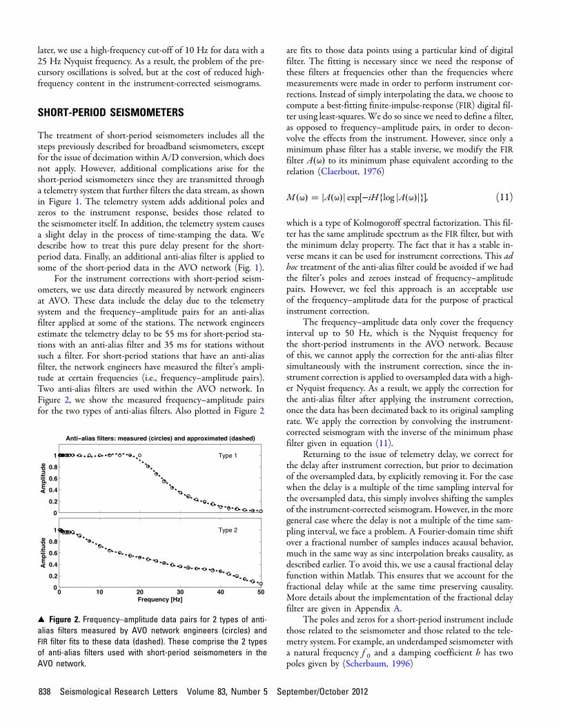
For the instrument corrections with short-period seism-ometers, we use data directly measured by network engineersat AVO. These data include the delay due to the telemetrysystem and the frequency–amplitude pairs for an anti-aliasfilter applied at some of the stations. The network engineersestimate the telemetry delay to be 55 ms for short-period sta-tions with an anti-alias filter and 35 ms for stations withoutsuch a filter. For short-period stations that have an anti-aliasfilter, the network engineers have measured the filter’s ampli-tude at certain frequencies (i.e., frequency–amplitude pairs).Two anti-alias filters are used within the AVO network. InFigure 2, we show the measured frequency–amplitude pairsfor the two types of anti-alias filters. Also plotted in Figure 2

are fits to those data points using a particular kind of digitalfilter. The fitting is necessary since we need the response ofthese filters at frequencies other than the frequencies wheremeasurements were made in order to perform instrument cor-rections. Instead of simply interpolating the data, we choose tocompute a best-fitting finite-impulse-response (FIR) digital fil-ter using least-squares. We do so since we need to define a filter,as opposed to frequency–amplitude pairs, in order to decon-volve the effects from the instrument. However, since only aminimum phase filter has a stable inverse, we modify the FIRfilter A�ω� to its minimum phase equivalent according to therelation (Claerbout, 1976)

M�ω� � jA�ω�j exp�−iHflog jA�ω�jg�; (11)

which is a type of Kolmogoroff spectral factorization. This fil-ter has the same amplitude spectrum as the FIR filter, but withthe minimum delay property. The fact that it has a stable in-verse means it can be used for instrument corrections. This adhoc treatment of the anti-alias filter could be avoided if we hadthe filter’s poles and zeroes instead of frequency–amplitudepairs. However, we feel this approach is an acceptable useof the frequency–amplitude data for the purpose of practicalinstrument correction.

The frequency–amplitude data only cover the frequencyinterval up to 50 Hz, which is the Nyquist frequency forthe short-period instruments in the AVO network. Becauseof this, we cannot apply the correction for the anti-alias filtersimultaneously with the instrument correction, since the in-strument correction is applied to oversampled data with a high-er Nyquist frequency. As a result, we apply the correction forthe anti-alias filter after applying the instrument correction,once the data has been decimated back to its original samplingrate. We apply the correction by convolving the instrument-corrected seismogram with the inverse of the minimum phasefilter given in equation (11).

Returning to the issue of telemetry delay, we correct forthe delay after instrument correction, but prior to decimationof the oversampled data, by explicitly removing it. For the casewhen the delay is a multiple of the time sampling interval forthe oversampled data, this simply involves shifting the samplesof the instrument-corrected seismogram. However, in the moregeneral case where the delay is not a multiple of the time sam-pling interval, we face a problem. A Fourier-domain time shiftover a fractional number of samples induces acausal behavior,much in the same way as sinc interpolation breaks causality, asdescribed earlier. To avoid this, we use a causal fractional delayfunction within Matlab. This ensures that we account for thefractional delay while at the same time preserving causality.More details about the implementation of the fractional delayfilter are given in Appendix A.

The poles and zeros for a short-period instrument includethose related to the seismometer and those related to the tele-metry system. For example, an underdamped seismometer witha natural frequency f 0 and a damping coefficient h has twopoles given by (Scherbaum, 1996)

▴ Figure 2. Frequency–amplitude data pairs for 2 types of anti-alias filters measured by AVO network engineers (circles) andFIR filter fits to these data (dashed). These comprise the 2 typesof anti-alias filters used with short-period seismometers in theAVO network.

838 Seismological Research Letters Volume 83, Number 5 September/October 2012

p1;2 � −2πf 0�h� i�������������1 − h2

p� (12)

and two zeros at 0 Hz. Note that for an underdamped seism-ometer h < 1. In addition to these poles, there are other polesrelated to the telemetry system. In the AVO network, the tele-metry is composed of a voltage-controlled oscillator (McChes-ney, 1999) and a discriminator. These act as the send andreceive components in the radio communication. Both of thesecomponents are modeled as low-pass Butterworth filters with acorner frequency at 30 Hz. Therefore, the additional poles arethose computed for a low-pass Butterworth filter. Using theseanalog poles and zeros, we proceed by applying the bilineartransform to compute digital poles and zeros just as in the caseof the broadband seismometers described earlier.

DATA EXAMPLE AND MATLAB CODES

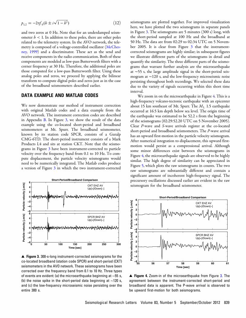
We now demonstrate our method of instrument correctionwith original Matlab codes and a data example from theAVO network. The instrument correction codes are describedin Appendix B. In Figure 3, we show the result of the dataexample using the co-located short-period and broadbandseismometers at Mt. Spurr. The broadband seismometer,known by its station code SPCR, consists of a GuralpCMG-6TD. The short-period instrument consists of a MarkProducts L4 and sits at station CKT. Note that the seismo-grams in Figure 3 have been instrument-corrected to particlevelocity over the frequency band from 0.1 to 10 Hz. To com-pute displacement, the particle velocity seismograms wouldneed to be numerically integrated. The Matlab codes producea version of Figure 3 in which the two instrument-corrected

seismograms are plotted together. For improved visualizationhere, we have plotted the two seismograms in separate panelsin Figure 3. The seismograms are 5 minutes (300 s) long, withthe short-period sampled at 100 Hz and the broadband at50 Hz. The data are from 02:29 to 02:34 UTC on 5 Novem-ber 2005. It is clear from Figure 3 that the instrument-corrected seismograms are highly similar; in subsequent figureswe illustrate different parts of the seismograms in detail andquantify the similarity. The three different parts of the seismo-grams that warrant further analysis are the microearthquakeat ∼55 s, the large amplitude signal in the short-period seis-mogram at ∼120 s, and the low-frequency microseismic noisepersisting throughout both recordings. We selected these datadue to the variety of signals occurring within this short timeinterval.

We zoom in on the microearthquake in Figure 4. This is ahigh-frequency volcano-tectonic earthquake with an epicenterabout 15 km southeast of Mt. Spurr. The ML 1.5 earthquakeoccurred at 16.5 km depth below sea level. The origin time ofthe earthquake was estimated to be 52.2 s from the beginningof the seismograms (02:29:52.20 UTC on 5 November 2005).Clear P-wave and S-wave arrivals register at the co-locatedshort-period and broadband seismometers. The P-wave arrivalhas an upward first-motion in the particle velocity seismogram.After numerical integration to displacement, this upward first-motion would persist as a compressional arrival. Althoughsome minor differences exist between the seismograms inFigure 4, the microearthquake signals are observed to be highlysimilar. The high degree of similarity can be appreciated inFigure 5, which plots the raw seismograms in counts. The tworaw seismograms are substantially different and contain asignificant amount of incoherent high-frequency signal. Theprecursory oscillations discussed earlier are evident in the rawseismogram for the broadband seismometer.

▴ Figure 3. 300-s-long instrument-corrected seismograms for theco-located broadband (station code SPCR) and short-period (CKT)seismometers in the AVO network. These seismograms have beencorrected over the frequency band from 0.1 to 10 Hz. Three typesof events are evident: (a) the microearthquake beginning at ∼55 s,(b) the noise spike in the short-period data beginning at ∼120 s,and (c) the low-frequency microseismic noise persisting over theentire 300 s.

▴ Figure 4. Zoom-in of the microearthquake from Figure 3. Theagreement between the instrument-corrected short-period andbroadband data is apparent. The P-wave arrival is observed tobe upward first-motion for both seismograms.

Seismological Research Letters Volume 83, Number 5 September/October 2012 839

We zoom in on the large amplitude signal occurring at∼120 s time in the short-period seismogram in Figure 6.Although we do not plot it here, the raw seismogram for theshort-period instrument contains a single large, negative ampli-tude data point at this same time. This is indicative of a noisespike due to the radio telemetry system that the short-periodinstrument passes through. The noise spike is not related to theinstrument response and so it results in high-amplitude noisein the instrument-corrected seismogram. Interestingly, the in-strument-corrected signal arising from the spike can be consid-ered to be an approximation of the “impulse response” of theinstrument-correction filter. As seen in Figure 6, the approx-imate impulse response has a sharp onset and reverberatesafterward, a consequence of the causal property of the instru-ment correction.

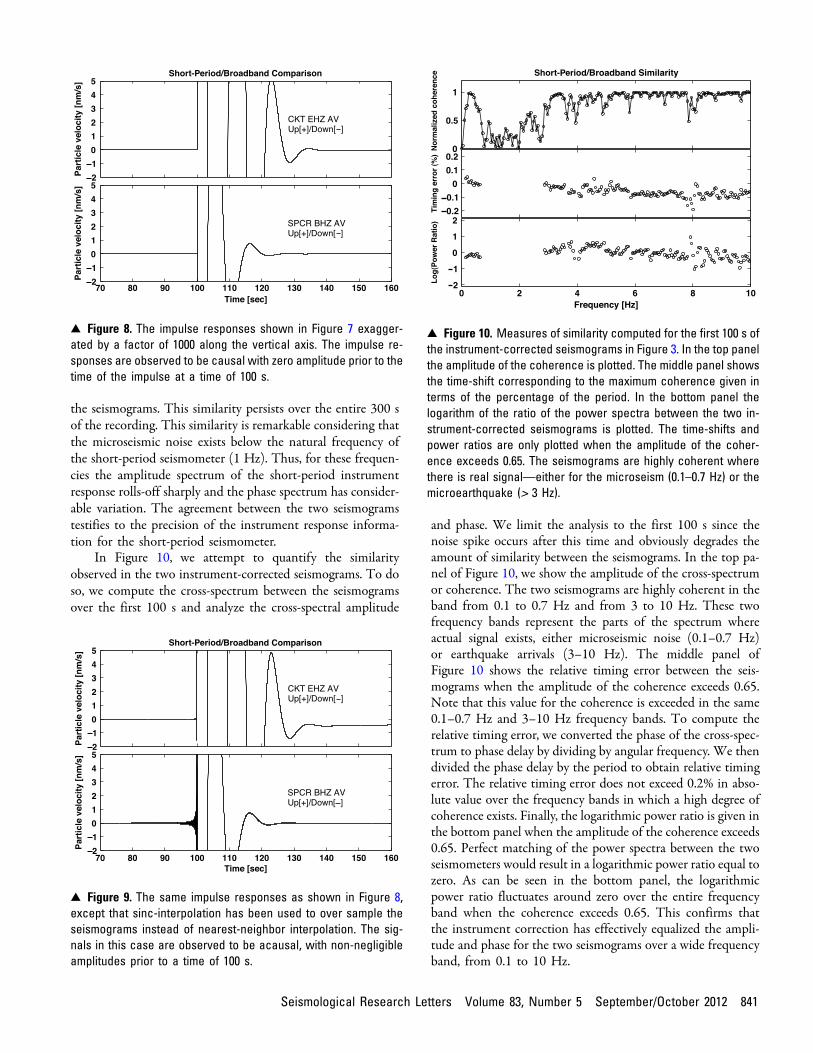
In Figures 7 through 9, we further explore this issue byexamining the actual impulse response of the instrument-correction filters for both the short-period and broadbandseismometers. A comparison of the impulse responses is shownin Figure 7 for an impulse at a time of 100 s. The impulseresponse for the broadband seismometer SPCR more closelyapproximates an ideal impulse than the impulse responsefor the short-period seismometer CKT. Note the similaritybetween the impulse response for CKT and the instrument-corrected noise spike in Figure 6. In Figure 8, we re-plotFigure 7 but with a vertical axis exaggerated by a factor of1000. We show the plot in Figure 8 in order to emphasize thecausal property of the impulse response; that is, the instrument-corrected seismogram is zero prior to the impulse at a time of100 s. This brings up the issue we discussed earlier concerningwhich interpolation scheme should be used for oversampling:sinc or nearest-neighbor. The plot in Figure 8 is the result for

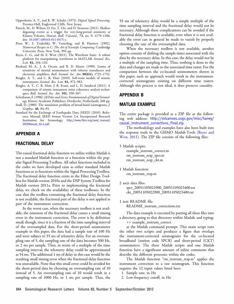
our preferred interpolation scheme, nearest-neighbor. InFigure 9, we show the same plot as in Figure 8 expect that weuse sinc interpolation for oversampling. As we argued earlier,sinc interpolation results in an acausal instrument-correction,as seen by comparing Figures 8 and 9. From these figures, weconclude that the instrument corrections we have designed areindeed causal.

Returning to Figure 6, we note the high degree ofsimilarity for the continuous microseismic noise between

▴ Figure 5. Zoom-in of the same time period as shown in Figure 4,but for the raw seismograms. The signal from the microearthquakeis seen to be vastly different between the two instruments prior toinstrument correction. High-frequency precursory oscillations areevident in the raw seismogram for the broadband instrument(SPCR).

▴ Figure 6. Zoom-in of the noise spike shown in Figure 3. Thenoise spike in the raw data is simply a single high-amplitude datapoint. After instrument correction, the impulse response of the in-strument correction filter appears. The fact that this signal is one-sided in essence proves that the instrument correction is causal.The background microseismic noise is also observed to be highlyconsistent between the two seismometers.

▴ Figure 7. The impulse response of the instrument correctionfilter for both the short-period (CKT) and broadband (SPCR) seism-ometers. The impulse for this example occurs at a time of 100 s.Note the similarity of the impulse response for short-period stationCKT to the signal in Figure 6.

840 Seismological Research Letters Volume 83, Number 5 September/October 2012

the seismograms. This similarity persists over the entire 300 sof the recording. This similarity is remarkable considering thatthe microseismic noise exists below the natural frequency ofthe short-period seismometer (1 Hz). Thus, for these frequen-cies the amplitude spectrum of the short-period instrumentresponse rolls-off sharply and the phase spectrum has consider-able variation. The agreement between the two seismogramstestifies to the precision of the instrument response informa-tion for the short-period seismometer.

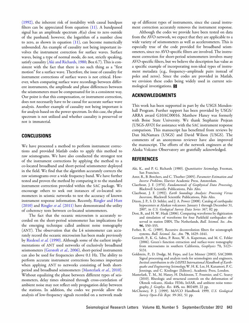
In Figure 10, we attempt to quantify the similarityobserved in the two instrument-corrected seismograms. To doso, we compute the cross-spectrum between the seismogramsover the first 100 s and analyze the cross-spectral amplitude

and phase. We limit the analysis to the first 100 s since thenoise spike occurs after this time and obviously degrades theamount of similarity between the seismograms. In the top pa-nel of Figure 10, we show the amplitude of the cross-spectrumor coherence. The two seismograms are highly coherent in theband from 0.1 to 0.7 Hz and from 3 to 10 Hz. These twofrequency bands represent the parts of the spectrum whereactual signal exists, either microseismic noise (0.1–0.7 Hz)or earthquake arrivals (3–10 Hz). The middle panel ofFigure 10 shows the relative timing error between the seis-mograms when the amplitude of the coherence exceeds 0.65.Note that this value for the coherence is exceeded in the same0.1–0.7 Hz and 3–10 Hz frequency bands. To compute therelative timing error, we converted the phase of the cross-spec-trum to phase delay by dividing by angular frequency. We thendivided the phase delay by the period to obtain relative timingerror. The relative timing error does not exceed 0.2% in abso-lute value over the frequency bands in which a high degree ofcoherence exists. Finally, the logarithmic power ratio is given inthe bottom panel when the amplitude of the coherence exceeds0.65. Perfect matching of the power spectra between the twoseismometers would result in a logarithmic power ratio equal tozero. As can be seen in the bottom panel, the logarithmicpower ratio fluctuates around zero over the entire frequencyband when the coherence exceeds 0.65. This confirms thatthe instrument correction has effectively equalized the ampli-tude and phase for the two seismograms over a wide frequencyband, from 0.1 to 10 Hz.

▴ Figure 9. The same impulse responses as shown in Figure 8,except that sinc-interpolation has been used to over sample theseismograms instead of nearest-neighbor interpolation. The sig-nals in this case are observed to be acausal, with non-negligibleamplitudes prior to a time of 100 s.

▴ Figure 10. Measures of similarity computed for the first 100 s ofthe instrument-corrected seismograms in Figure 3. In the top panelthe amplitude of the coherence is plotted. The middle panel showsthe time-shift corresponding to the maximum coherence given interms of the percentage of the period. In the bottom panel thelogarithm of the ratio of the power spectra between the two in-strument-corrected seismograms is plotted. The time-shifts andpower ratios are only plotted when the amplitude of the coher-ence exceeds 0.65. The seismograms are highly coherent wherethere is real signal—either for the microseism (0.1–0.7 Hz) or themicroearthquake (> 3 Hz).

▴ Figure 8. The impulse responses shown in Figure 7 exagger-ated by a factor of 1000 along the vertical axis. The impulse re-sponses are observed to be causal with zero amplitude prior to thetime of the impulse at a time of 100 s.

Seismological Research Letters Volume 83, Number 5 September/October 2012 841

We further investigate the coherency of instrument-corrected signals between the co-located seismometers inFigure 11 by analyzing a regional earthquake instead of a localmicroearthquake. We perform this test to check whether thecoherency is high in the frequency band from 1 to 3 Hz thatlacked signal in Figure 10. A regional earthquake has a broaderspectrum than a local microearthquake and should have signalwithin this band. As seen in Figure 11, the coherency for theregional earthquake is high for all frequencies above 0.1 Hz.Since the frequency content of the signal is more continuousthan that of the microearthquake considered previously, asubtle linear trend is evident in the relative timing between thetwo instruments, as shown in the middle panel. This smalltrend may represent the limits of the precision with whichthe timing, or the phase portion of the instrument response,is known for these instruments. The logarithmic power ratio inthe bottom panel demonstrates that the power spectra for thetwo signals are highly similar.

Finally, in Figure 12 we compare instrument-correctedseismograms for the broadband station SPCR using the meth-od we have developed in this paper and the SAC commandTRANSFER. An important detail is that to produce a causalinstrument response, the SAC commands must be executed in aspecific and non-standard way. This issue is discussed inAppendix C. As shown in Figure 12, our method for instru-ment correction and SAC produce highly similar results for themicroearthquake plotted in Figure 4. This validates ourmethod against the widely used SAC instrument correctioncapabilities. Furthermore, we have found a suitable sequence ofSAC commands for producing a causal instrument correction.

We wish to point out that an effort must be made on thepart of the users of the provided codes to preserve the causalproperty of the instrument corrections in subsequent proces-sing of the particle velocity seismograms. For instance, numer-ical integration to displacement is causal but often a low-frequency noise or drift exists afterward. The usual approachto this problem is to apply a high-pass filter after numericalintegration. The high-pass filter in this case would need tobe causal itself. This also applies to any band-pass filteringof the instrument-corrected seismograms. We have limitedthe discussion of instrument correction in this paper to thecentral step of converting from counts to particle velocity.We leave subsequent integration or filtering to the discretionof the user.

DISCUSSION

In this paper, the overriding goal has been to forge a method forinstrument correction that preserves the property of causality.The data examples described above show that we have achievedthis goal. Certainly, the preservation of causality makes sensefor real seismic signals—the seismometer does not begin toshake prior to the arrival of seismic waves. However, onemay wonder about the drawbacks of a causal instrument cor-rection. Are there times when a causal instrument correction isnot preferred, does not work well, or is not important? Regard-ing this issue, the main drawback to a causal instrumentcorrection is that it can be prone to numerical instability,for the reasons discussed earlier regarding the low-pass andhigh-pass Butterworth filters. As discussed by Claerbout

▴ Figure 11. Measures of similarity, as in Figure 10, except com-puted for a regional earthquake instead of a local microearth-quake. In the top panel the amplitude of the coherence isplotted. The middle panel shows the time-shift correspondingto the maximum coherence given in terms of the percentage ofthe period. In the bottom panel the logarithm of the ratio of thepower spectra between the two instrument-corrected seismo-grams is plotted. The time-shifts and power ratios are only plottedwhen the amplitude of the coherence exceeds 0.65.

▴ Figure 12. Comparison between the method presented in thispaper (upper panel) and the instrument correction from SAC (lowerpanel) for the microearthquake in Figure 4. The agreement ob-served between the two instrument-corrected seismograms ex-tends over the entire time window, although here we highlightthe microearthquake. Note that the SAC instrument correctionhad to be performed in a non-standard way in order to preservecausality, as discussed in Appendix C.

842 Seismological Research Letters Volume 83, Number 5 September/October 2012

(1992), the inherent risk of instability with causal bandpassfilters can be appreciated from equation (11). A bandpassedsignal has an amplitude spectrum A�ω� close to zero outsideof the passband; however, the logarithm of a number closeto zero, as shown in equation (11), can become numericallyunbounded. An example of causality not being important in-volves the instrument correction for surface waves. Surfacewaves, being a type of normal mode, do not, strictly speaking,satisfy causality (Aki and Richards, 1980; Box 6.7). This is con-sistent with the fact that there is no such thing as a “firstmotion” for a surface wave. Therefore, the issue of causality forinstrument corrections of surface waves is not critical. How-ever, when comparing surface wave recordings between differ-ent instruments, the amplitude and phase differences betweenthe seismometers must be compensated for in a consistent way.Our point is that this compensation, or instrument correction,does not necessarily have to be causal for accurate surface waveanalysis. Another example of causality not being important isfor analysis based on the power spectrum. In this case, the phasespectrum is not utilized and whether causality is preserved ornot is immaterial.

CONCLUSIONS

We have presented a method to perform instrument correc-tions and provided Matlab codes to apply this method toraw seismograms. We have also conducted the strongest testof the instrument corrections by applying the method to aco-located broadband and short-period seismometer deployedin the field. We find that the algorithm accurately corrects theraw seismograms over a wide frequency band. We have furthertested and proven the method by comparing it to the standardinstrument correction provided within the SAC package. Weencourage others to seek out instances of co-located seis-mometers in seismic networks to test the accuracy of knowninstrument response information. Recently, Ringler and Hutt(2010) and Ringler et al. (2011) have demonstrated the utilityof coherency tests between co-located seismometers.

The fact that the oceanic microseism is accurately re-corded on the short-period seismometer has implications forthe emerging technique called ambient noise tomography(ANT). The observation that the L4 seismometer can accu-rately record the oceanic microseism has been made previouslyby Riedesel et al. (1990). Although some of the earliest imple-mentations of ANT used networks of exclusively broadbandseismometers (Gerstoft et al., 2006), short-period instrumentscan also be used for frequencies above 0.1 Hz. The ability toperform accurate instrument corrections becomes importantwhen applying ANT to networks consisting of both short-period and broadband seismometers (Masterlark et al., 2010).Without equalizing the phase between different types of seis-mometers, delay times obtained through cross-correlation ofambient noise may not reflect only propagation delay betweenthe stations. In addition, the codes we provide allow theanalysis of low-frequency signals recorded on a network made

up of different types of instruments, since the causal instru-ment correction accurately removes the instrument response.

Although the codes we provide have been tested on datafrom the AVO network, we expect that they are applicable to awide variety of seismometers as well as accelerometers. This isespecially true of the code provided for broadband seism-ometers, since no AVO-specific filters are involved. The instru-ment correction for short-period seismometers involves manyAVO-specific filters, but we believe the description has value asa specific example of incorporating non-ideal types of instru-ment metadata (e.g., frequency–amplitude pairs instead ofpoles and zeros). Since the codes are provided in Matlab,we envision these codes being widely used in current seis-mological investigations.

ACKNOWLEDGMENTS

This work has been supported in part by the USGS Menden-hall Program. Further support has been provided by USGS/ARRA award G10AC00016. Matthew Haney was formerlywith Boise State University. We thank Stephanie Prejean(USGS-AVO) for assistance with the SAC instrument responsecomparison. This manuscript has benefitted from reviews byDan McNamara (USGS) and David Wilson (USGS). Thecomments of an anonymous reviewer have also improvedthe manuscript. The efforts of the network engineers at theAlaska Volcano Observatory are gratefully acknowledged.

REFERENCES

Aki, K., and P. G. Richards (1980). Quantitative Seismology, Freeman,San Francisco.

Aster, R., B. Borchers, and C. Thurber (2005). Parameter Estimation andInverse Problems, Elsevier Academic Press, Amsterdam.

Claerbout, J. F. (1976). Fundamentals of Geophysical Data Processing,Blackwell Scientific Publications, Palo Alto.

Claerbout, J. F. (1992). Earth Soundings Analysis: Processing VersusInversion, Blackwell Scientific Publications, Palo Alto.

Dixon, J. P., S. D. Stihler, and J. A. Power (2008). Catalog of earthquakehypocenters at Alaskan volcanoes: January 1 through December 31,2007, in U.S. Geological Survey Data Series 367, 82 pp.

Dost, B., and H. W. Haak (2006). Comparing waveforms by digitizationand simulation of waveforms for four Parkfield earthquakes ob-served in station DBN, The Netherlands, Bull. Seismol. Soc. Am.96, S50–S55.

Ferber, R. -G. (1989). Recursive deconvolution filters for seismographsystems, Bull. Seismol. Soc. Am. 79, 1629–1641.

Gerstoft, P., K. G. Sabra, P. Roux, W. A. Kuperman, and M. C. Fehler(2006). Green’s function extraction and surface-wave tomographyfrom microseisms in southern California, Geophysics 71, S123–S131.

Goldstein, P., D. Dodge, M. Firpo, and Lee Minner (2003). SAC2000:Signal processing and analysis tools for seismologists and engineers,Invited contribution to the IASPEI International Handbook of Earth-quake and Engineering Seismology,W. H. K. Lee, H. Kanamori, P. C.Jennings, and C. Kisslinger (Editors), Academic Press, London.

Masterlark, T. M., M. Haney, H. Dickinson, T. Fournier, and C. Searcy(2010). Rheologic and structural controls on the deformation ofOkmok volcano, Alaska: FEMs, InSAR, and ambient noise tomo-graphy, J. Geophys. Res. 115, no. B02409, 22 pp.

McChesney, P. J. (1999). McVCO Handbook 1999, U.S. GeologicalSurvey Open-File Rept. 99-361, 51 pp.

Seismological Research Letters Volume 83, Number 5 September/October 2012 843

Oppenheim, A. V., and R. W. Schafer (1975). Digital Signal Processing,Prentice-Hall, Englewood Cliffs, New Jersey.

Patrick, M., D. Wilson, D. Fee, T. Orr, and D. Swanson (2011). Shallowdegassing events as a trigger for very-long-period seismicity atKilauea Volcano, Hawaii, Bull. Volcanol., 73, no. 9, 1179–1186,doi: 10.1007/s00445-011-0475-y.

Press, W., S. Teukolsky, W. Vetterling, and B. Flannery (1992).Numerical Recipes in C: The Art of Scientific Computing, CambridgeUniversity Press, New York, 994 pp.

Reyes, C. G., and M. E. West (2011). The Waveform Suite: A robustplatform for manipulating waveforms in MATLAB, Seismol. Res.Lett. 82, 104–110.

Riedesel, M. A., J. A. Orcutt, and R. D. Moore (1990). Limits ofsensitivity of inertial seismometers with velocity transducers andelectronic amplifiers, Bull. Seismol. Soc. Am. 80(6A), 1725–1752.

Ringler, A. T., and C. R. Hutt (2010). Self-noise models of seismicinstruments, Seismol. Res. Lett. 81, 972–983.

Ringler, A. T., C. R. Hutt, J. R. Evans, and L. D. Sandoval (2011). Acomparison of seismic instrument noise coherence analysis techni-ques, Bull. Seismol. Soc. Am. 101, 558–567.

Scherbaum, F. (1996).Of Poles and Zeros: Fundamentals of Digital Seismol-ogy, Kluwer Academic Publishers, Dordrecht, Netherlands, 268 pp.

Seidl, D. (1980). The simulation problem of broad-band seismograms, J.Geophys. 48, 84–93.

Standard for the Exchange of Earthquake Data (SEED) (2010). Refer-ence Manual, SEED format Version 2.4, Incorporated ResearchInstitution for Seismology, http://www.fdsn.org/seed_manual/SEEDManual_V2.4.pdf.

APPENDIX A

FRACTIONAL DELAY

The causal fractional delay function we utilize within Matlab isnot a standard Matlab function or a function within the pop-ular Signal Processing Toolbox. All other functions included inthe codes we have developed exist as either standard Matlabfunctions or as functions within the Signal ProcessingToolbox.The fractional delay function exists in the Filter Design Tool-box forMatlab version 2010a and the DSP System Toolbox forMatlab version 2011a. Prior to implementing the fractionaldelay, we check on the availability of these toolboxes. In thecase that the toolbox containing the fractional delay functionis not available, the fractional part of the delay is not applied aspart of the instrument correction.

In the worst case, when the necessary toolbox is not avail-able, the omission of the fractional delay causes a small timingerror in the instrument correction. The error is by definitionsmall, though, since it is a fraction of the time sampling intervalof the oversampled data. For the short-period seismometerexample in this paper, the data had a sample rate of 100 Hzand were subject to 55 ms of telemetry delay. For an oversam-pling rate of 5, the sampling rate of the data becomes 500 Hz,or 2 ms per sample. Thus, in terms of a multiple of the timesampling interval, the telemetry delay could be approximatedas 54 ms. The additional 1 ms of delay in this case would be theresulting small timing error when the fractional delay functionwas unavailable. Note that this small error could be avoided forthe short-period data by choosing an oversampling rate of 10instead of 5. An oversampling rate of 10 would result in asampling rate of 1000 Hz, or 1 ms per sample. Thus, the

55 ms of telemetry delay would be a simple multiple of thetime sampling interval and the fractional delay would not benecessary. Although these complications can be avoided if thefractional delay function is available, even when it is not avail-able the error can in general be made to vanish by properlychoosing the rate of the oversampled data.

When the necessary toolbox is not available, anotheroption consists of shifting the sample times associated with thedata by the necessary delay. In this case, the delay would not bea multiple of the sampling time. Thus, nothing is done to thedata and changes are made to the associated time raster. For thecomparison between the co-located seismometers shown inthis paper, such an approach would result in the instrument-corrected seismograms existing on different time rasters.Although this process is not ideal, it does preserve causality.

APPENDIX B

MATLAB EXAMPLE

The entire package is provided as a ZIP file at the follow-ing web address: http://volcanoes.usgs.gov/misc/haney/causal_instrument_corrections_final.zip.

The methodology and examples have also been built intothe response tools in the GISMO Matlab Tools (Reyes andWest, 2011). The ZIP file consists of the following files:

3 Matlab scripts:example_instrum_correct.mrm_instrum_resp_spcr.mrm_instrum_resp_ckt.m

1 Matlab function:rm_instrum_resp.m

2 ascii data files:spcr_20051105022900_20051105023400.txtckt_20051105022900_20051105023400.txt

1 text README file:README_instrum_corrections.txt

The data example is executed by putting all these files intoa directory, going to that directory within Matlab, and typing:

>> example_instrum_correctat the Matlab command prompt. This main script runs

the other two scripts and produces a figure that overlapsthe instrument-corrected seismograms for the co-locatedbroadband (station code SPCR) and short-period (CKT)seismometers. The three Matlab scripts and one Matlabfunction have a significant amount of inline comments thatdescribe the different processes within the codes.

The Matlab function “rm_instrum_resp.m” applies theinstrument correction to a raw seismogram. This functionrequires the 12 input values listed here:1. Sample rate, in Hz2. Low-frequency cutoff, in Hz

844 Seismological Research Letters Volume 83, Number 5 September/October 2012

3. Order of the high-pass Butterworth filter4. High-frequency cutoff, in Hz5. Order of the low-pass Butterworth filter6. Bad data value7. Analog zeros, in rad=s8. Analog poles, in rad=s9. Inverse gain 1=G, in m/s/count10. Reference frequency f R, in Hz11. Oversampling rate (� 5 by default)12. Intrinsic system delay, in ms (� 0 s for broadbands, 35 ms

or 55 ms for AVO short-periods)

The 6th input parameter, the bad data value, refers to thevalue given to samples in the seismogram when no data arereceived (e.g., a telemetry dropout). In the acquisition systemused by the AVO network, this value is set to the most negative32-bit integer, −2∧31. By forcing the user to specify this, weintend to keep the user aware that our Matlab instrument cor-rection codes do not solve the “missing data” problem. It is upto the user to somehow fill in the missing data according to acertain methodology before using these codes. By specifying abad data value and then attempting to run the codes on a rawseismogram with bad data, the codes will give an error messageand stop. All other input parameters have been discussed al-ready in this paper. Note that it is important to be aware thatthe analog poles and zeros are to be given in angular frequency(radians/s) instead of linear frequency (Hz).

APPENDIX C

SAC INSTRUMENT CORRECTION

To apply a causal instrument correction in SAC, we executethe following series of commands on the raw seismogram,which for this example has the filename SPCR.BHZ.AV:

SAC> r SPCR.BHZ.AVSAC> rmeanSAC> rtrSAC> taper width 0.05SAC> lowpass npoles 5 corner 10SAC> rmeanSAC> rtrSAC> taper width 0.05SAC> highpass npoles 3 corner 0.1SAC> rmeanSAC> rtrSAC> taper width 0.05SAC> trans from evalresp to velSAC> rmeanSAC> rtr

SAC> taper width 0.05SAC> w SPCR.BHZ.AV.corr

These series of SAC commands can be combined in a sin-gle SAC macro file. Note that the trans command requires thepresence of a RESP file in the directory for station SPCR. TheRESP file, called RESP.AV.SPCR..BHZ, can be obtained fromthe AVO miniseed available on the IRIS website. The RESPfile for SPCR is also available at: http://www.iris.edu/mda/AV/SPCR

In the above instance of the trans command, we deliber-ately avoid using the freqlimits option that is commonlyinvoked with this SAC command. The freqlimits option is in-tended to define a passband over which the instrument-corrected seismogram is returned. However, as implementedin SAC, the freqlimits option uses a two-pass, zero-phase filterinstead of a one-pass, causal filter. This fact is pointed out inthe SAC Users Manual. Thus, the instrument-corrected seis-mogram returned after invoking the freqlimits option is acau-sal. To define a passband while also ensuring a causal responsewithin SAC, we have elected to apply causal high-pass and low-pass filters prior to correcting with the trans command. Thehigh- and low-frequency corners of these filters, respectively10 Hz and 0.1 Hz, and number of poles have been chosento match the example in this paper. Finally, we generouslyutilize tapering, mean removal, and trend removal prior to andfollowing all filtering steps. Employing these additional stepsensures that instabilities and errors due to the finite length ofthe seismogram are avoided.

Matthew M. HaneyJohn Power

Alaska Volcano ObservatoryVolcano Science CenterU.S. Geological Survey

Anchorage, Alaska 99508 U.S.A.

Michael WestAlaska Volcano Observatory

Geophysical InstituteUniversity of Alaska Fairbanks

Fairbanks, Alaska 99775 U.S.A.

Paul MichaelsCenter for Geophysical Investigation of theShallow Subsurface

Department of GeosciencesBoise State University

Boise, Idaho 83725 U.S.A.

Seismological Research Letters Volume 83, Number 5 September/October 2012 845