CAUSALITY CORRECTIONS IMPLEMENTED IN 2nd PRINTING

CONTENTS 1

CAUSALITY CORRECTIONSIMPLEMENTED IN 2nd PRINTING

Updated 9/26/00

page v insert “TO RUTH” centered in middle of page

page xv insert in second paragraph “David Galles” after “Dechter”

page 2 replace “2000” with “2004” in 2nd paragraph, line 8 of 1.1.2

page 3 insert “, � ” after “( � )” in footnote 1*replace* “and not” with “not, and implies,” in footnote 1

page 19 *append* (continue italics) to end of Theorem 1.2.7, “(We exclude �� when

speaking of its “nondescendants”.)”

page 30 replace in line 7 from top “mutually” with “jointly”*insert* “parental” before “Markov” in first line of 2nd paragraph after Theorem1.4.1*append* to end of footnote 16 “but I am not aware of any nonparametric version.”

page 52 insert “stable” after “IC*, that takes a” in 2nd paragraph after Theorem 2.6.2,*replace* “sampled” with “stable” in Input line of IC* Algorithm.*append* “(with respect to some latent structure).” to same line

page 52 page 55, 1st line of footnote 9replace “Pearl (1990)” with “Pearl (1990a)”

page 68 replace in line 1 after Eq. (3.2), “mutually” with “jointly”

page 72 replace “(1990, 1999)” with “(1990, 2001)” on line 6

page 89 replace in paragraph starting “Indeed, if condition...”. Should be “conditionsrequire” not “condition require”

page 126 insert “and Robins (1997)” after “Pearl and Robins (1995)”, line 2.

page 130 replace the “ � ” with “ � ” in the formula (second line of section 4.5.4.) Shouldread “ � �� ”*replace* “we can compute the difference” with “we should replace the controlleddifference” in last line of page

2 CONTENTS

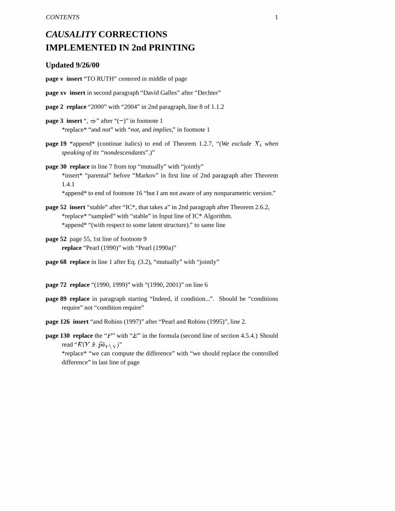
page 131 replace from top of page through the end of section 4.5.4 with the following:

� �� with some average of this difference over all departments. This average should mea-sure the increase in admission rate in a hypothetical experiment in which we instructall female candidates to retain their department preferences but change their genderidentification (on the application form) from female to male.

In general, the average direct effect is defined as the expected change in � inducedby changing � from � to � � while keeping the other parents of � constant at what-ever value they obtain under �� . This hypothetical change is what law makersinstruct us to consider in race or sex discrimination cases: “The central question inany employment-discrimination case is whether the employer would have taken thesame action had the employee been of a different race (age, sex, religion, nationalorigin etc.) and everything else had been the same.” (In Carson versus BethlehemSteel Corp., 70 FEP Cases 921, 7th Cir. (1996)).

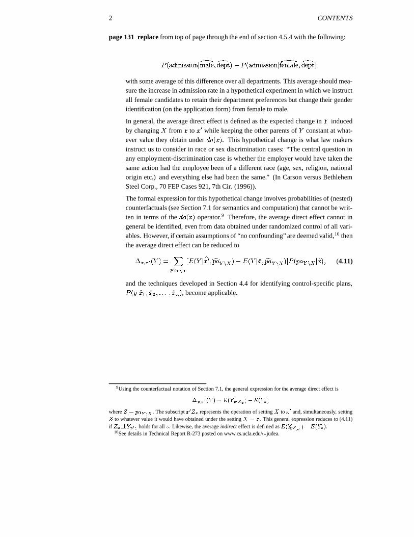
The formal expression for this hypothetical change involves probabilities of (nested)counterfactuals (see Section 7.1 for semantics and computation) that cannot be writ-ten in terms of the �� operator.9 Therefore, the average direct effect cannot ingeneral be identified, even from data obtained under randomized control of all vari-ables. However, if certain assumptions of “no confounding” are deemed valid,10 thenthe average direct effect can be reduced to!#"�$ "&% � � �(' )

*,+.-0/2143 � � � �5� � �� 6� � �� 87 � � �� (4.11)

and the techniques developed in Section 4.4 for identifying control-specific plans,� ��9 ��;: �� < ,=�=,= ��0> � , become applicable.

9Using the counterfactual notation of Section 7.1, the general expression for the average direct effect is?A@&B @ %8C�DFEHGJIAC�D @ %LKNM�E�OPIQC�D @ Ewhere R G�S�T,U;VXW . The subscript Y[Z�R @ represents the operation of setting \ to Y[Z and, simultaneously, settingR to whatever value it would have obtained under the setting \ G Y . This general expression reduces to (4.11)if R @[]^] D @ %`_ holds for all a . Likewise, the average indirect effect is defined as

IAC�D @ K M % E�O#IAC�D @ E.

10See details in Technical Report R-273 posted on www.cs.ucla.edu/ b judea.

CONTENTS 3

page 164 replace ... “ �� 9 �� ” with “ �� ” in line 8 after Definition 5.4.3.

page 165 replace last two sentences of section 5.4.2 with:The expressions corresponding to these policies are� ��9 �� and � ��9 �� , and this pair of distributions fully repre-sents the policy implications of indirect effects. Similar conclusions have beenexpressed by Robins and Greenland (1992). (But see Chapter 4, footnote 9, page131.)

page 177 *delete* “tormented” in paragraph 3, line 2

page 184 *append* to end of Definition 6.2.1 (continue italics - except ‘unbiased’): “If(6.10) holds, we say that � � 9 �� is unbiased.”

page 216 In line before Eq. (7.11), replace “To answer the first query,” with “In order toanswer the first query,”

page 236 replace “& � � � � ” with “& � � �� ” in first formula of Theorem

7.3.8

page 240 replace the last sentence in the last paragraph of section 7.4.1 with:However, this effectiveness is partly acquired by limiting the counterfactual an-tecedent to conjunction of elementary propositions. Disjunctive hypotheticals, suchas “if Bizet and Verdi were compatriots,” usually lead to multiple solutions and henceto nonunique probability assignments.

page 246 insert in footnote 26 after “(see Section 5.4.3).” “Epidemiologists refer to (7.46)as “no-confounding” (see (6.10)).”

page 255 replace in the 2nd line “pregnant” with “nonpregnant”

page 259 insert close parentheses after “(Sections 3.2 and 7.1”, line 2 of Preface

page 284 replace “Michie in press” with “Michie 1999” in the last line of paragraph 4

page 329 replace “(1999)” with “(2000)” in last line of page

page 332 replace in paragraph starting “Even an erratic and ...”. Change “role” to “roll”

page 354 line 2 from bottom, replace “mediated by tar deposits” with “unmediated by tardeposits”

page 361 *update* Dawid 1997 citation. replace “To appear ...” with “Also [with discus-sion] in Journal of the American Statistical Association 95:407–48, 2000.”

page 363 *append* to Halpern (1998) citation, “Also, Journal of Artificial Intelligence

Research 12:317–37, 2000.”*update* Halpern and Pearl (1999) citation. replace “(1999)” with “(2000)”,replace “Actual causality.” with “Causes and explanations.”, and *append*“www.cs.ucla.edu/ � judea/”

4 CONTENTS

page 364 *update* Hoover 1999 citation. replace “(1999)” with “(2001)”

page 365 *update* Kuroki citation. *append* “29: 105–17.” after “Journal of the JapanStatistical Society”.

page 366 *update* Michie citation. replace “(in press)” with “(1999)” and insert “pp.60-86” before “vol. 15”

page 368 *update* Pearl 1999 citation. *remove* “To appear in” and replace “121” with“121:93–149.”

page 369 insert in Robins 1997 citation, “M. Berkane (Ed.),” before “Latent Variable

Modeling...”

page 370 add* to Shipley 1997 citation, “Also in Structural Equation Modelling, 7:206–18, 2000.”

page 381 insert “27–8”, after “(examples) price and demand” and before “215-17”*replace* “245” with “245–7”, at end of “(exogeneity) controversies regard-ing...245”*combine* “explanation” and “explanations” to read “explanation, 25, 58, 221–3,285, 308–9”

page 382 insert “131” after “indirect effects,” and before “165”

CONTENTS 5

ADDENDUM TO CORRECTIONSIMPLEMENTED IN 2nd PRINTING

Updated 12/14/00

page 28 replace “income �� ” with “income �� ” in the caption of Figure 1.5

page 48 replace in line before Definition 2.4.1, “when one of the coins becomes slightlybiased.” with “when the coins become slightly biased.”

page 51 *append* to line 7, Rule �� to read:Orient � – � into � � � whenever there are two chains � – � � � and � � � � �such that � and � are nonadjacent and � and � are adjacent.

page 231 replace Definition 7.3.4 and 2 lines following to read:Definition 7.3.4 (Recursiveness)Let � and � be singleton variables in a model, and let � � � stand for theinequality � " �� ' � �� for some values of � �� , and � . A model is recursive

if, for any sequence � : � < �=,=�= �� , we have

� : � � < �� < � �� ,=�=�= � �� : � � � � � � �� : (7.24)

Clearly, any model for which the causal diagram � �� is acyclic must be recur-sive.

page 382 *change* “Markov (assumptions underlying, 30)” to “Markov (assumption, 30,69)”

page 382 *append* “69” after ”causal, 30” in “Markov condition (causal, 30)”

page 384 *add* as subentry after “structural model, 27, 44, 202” “Markovian, 30, 69”.

CONTENTS 1

PRINTING CORRECTIONS/ADDITIONSIN THE SECOND EDITION OF CAUSALITY

Updated 7/23/08

Preface

page v replace “TO RUTH” (centered in middle of title page) withTO DANNYAND THE AUDACITY OF GOODNESS(two lines indented and flushed left on title page)

page xvi Add new section to Preface.

Preface to the Second EditionIt has been more than eight years since the first edition of this book presented read-ers with the friendly face of causation and her mathematical artistry. The popularreception of the book and the rapid growth of the field call for a new edition to as-sist causation through her second transformation – from a demystified wonder to acommonplace tool in research and education. This edition (1) provides technicalcorrections, updates and clarifications in all ten chapters of the book, (2) adds sum-maries of new developments and annotated bibliographical references at the end ofeach chapter, and (3) elucidates subtle issues that readers and reviewers have foundperplexing, objectionable, or in need of elaboration. These are assembled into an en-tirely new chapter (11) which, I sincerely hope, clears the province of causal thinkingfrom the last traces of controversy.

Teachers who have taught from this book before should find the revised edition morelucid and palatable, while those who have waited for scouts to carve the path, willfind the road paved and tested. Supplementary educational material, slides, tutorialsand homeworks can be found on my website http://www.cs.ucla.edu/ � judea/.

My main audience remain the students: students of statistics who wonder whyinstructors are reluctant to discuss causality in class; students of epidemiologywho wonder why elementary concepts such as confounding are so hard to definemathematically; students of economics and social science who question the meaningof the parameters they estimate; and, naturally, students of artificial intelligence andcognitive science, who write programs and theories for knowledge discovery, causalexplanations and causal speech.

J.P.Los AngelesJuly 2008

2 CONTENTS

Chapter 1

page 9 -5 lines from bottom of pagereplace “ � " �� < � �� 9 � over all �� .” with“ � " �� 0� � < � �� 9 � over all possible �;� .”

page 11 add sentence to end footnote 4“Geiger and Pearl (1993) present an in-depth analysis.”

page 22 3 lines before footnote 8replace “join distribution” with “joint distribution”

page 24 line 7replace(iii) � " �� (' � �� for all �� whenever � � � is consistent with � ' � .with:(iii) � " �� (' � �� for all � � �� whenever � � � is consistent with � ' � ,i.e., each � �� remains invariant to interventions not involving � � .

page 31 footnote 18replace “such a property.” with “this property.”

page 32 2 lines before footnote 20replace ‘linear programming” with “linear-programming”

page 34 in 2nd linereplace “(Dawid 1997).” with “(Dawid 2000).”

page 39 Footnote 26, last sentencereplace Causal assumptions of the type developed in Chapter 2 (see Definitions 2.4.1and 2.7.4) must be invoked before applying such sequences in policy-related tasks.With:Such sequences are statistical in nature and, unless causal assumptions of the typedeveloped in Chapter 2 (see Definitions 2.4.1 and 2.7.4) are invoked, they cannot beapplied to policy-evaluation tasks.

replace first RemarkRemark: The distinction between probabilistic and statistical parameters is devisedto exclude the construction of joint distributions that invoke hypothetical variables(e.g., counterfactual or theological). Such constructions, if permitted, would qualifyany quantity as statistical and would obscure the distinction between causal and non-causal assumptions.With:Remark: The exclusion of unmeasured variables from the definition of statisticalparameters is devised to rule out the construction of joint distributions that invokecounterfactual or metaphysical variables. Such constructions, if permitted, wouldqualify any quantity as statistical and would thus obscure the important distinction

CONTENTS 3

between quantities that can be estimated from statistical data alone, and those thatrequire additional assumptions beyond the data.

insert (after “falsifiable”)Often, though not always, causal assumptions can be falsified from experimentalstudies, in which case we say that they are “experimentally testable.” For example,the assumption that � has no effect on � � � � in model 2 of Figure 1.6 is empiricallytestable, but the assumption that � may cure a given subject in the population is not.

replace second RemarkRemark: The distinction between causal and statistical parameters is crisp and fun-damental. Causal parameters can be discerned from joint distributions only whenspecial assumptions are made, and such assumptions must have causal componentsto them. The formulation and simplification of these assumptions will occupy a ma-jor part of this book.With:Remark: The distinction between causal and statistical parameters is crisp and fun-damental – the two do not mix. Causal parameters cannot be discerned from statisti-cal parameters unless causal assumptions are invoked. The formulation and simpli-fication of these assumptions will occupy a major part of this book.

page 40 Add to end of Chapter 1

Two Mental Barriers to Causal Analysis

The sharp distinction between statistical and causal concepts can be translated intoa useful principle: behind every causal claim there must lie some causal assumptionthat is not discernable from the joint distribution and, hence, not testable in observa-tional studies. Such assumptions are usually provided by humans, resting on expertjudgment. Thus, the way humans organize and communicate experiential knowledgebecomes an integral part of the study, for it determines the veracity of the judgmentsexperts are requested to articulate.

Another ramification of this causal-statistical distinction is that any mathematical ap-proach to causal analysis must acquire new notation. The vocabulary of probabilitycalculus, with its powerful operators of expectation, conditionalization and marginal-ization, is defined strictly in terms of distribution functions and is insufficient there-fore for expressing causal assumptions or causal claims. To illustrate, the syntax ofprobability calculus does not permit us to express the simple fact that “symptoms donot cause diseases,” let alone draw mathematical conclusions from such facts. Allwe can say is that two events are dependent—meaning that if we find one, we canexpect to encounter the other, but we cannot distinguish statistical dependence, quan-tified by the conditional probability � �� from causal dependence,for which we have no expression in standard probability calculus.

The preceding two requirements: (1) to commence causal analysis with untested,judgmental assumptions, and (2) to extend the syntax of probability calculus, consti-

4 CONTENTS

tute the two main obstacles to the acceptance of causal analysis among professionalswith traditional training in statistics (Pearl 2003b, 2008a; Cox and Wermuth 1996).This book helps overcome the two barriers through an effective and friendly nota-tional systems based on symbiosis of graphical and algebraic approaches.

Chapter 2

page 41 replace in line 5“is an outgrowth of Pearl (1988b, chap. 8), which describes”with“is an outgrowth of Rebane and Pearl (1987) (also, Pearl (1988b, Chap. 8), whichdescribes”

replace “On the other hand, the Stanford group” with “The Stanford group”

replace “to update the posterior probabilities assigned to” with “to update prior prob-abilities assigned to”

page 42 replace section heading, “2.1 INTRODUCTION” with “2.1 INTRODUCTION– THE BASIC INTUITIONS”

page 43 replace last two paragraphs of Section 2.1 withSuch thought experiments tell us that certain patterns of dependency, void of tempo-ral information, are conceptually characteristic of certain causal directionalities andnot others. Reichenbach (1956) who was the first to wonder about the origin of thosepatterns suggested that they are characteristic of Nature, reflective of the second lawof thermodynamics. Rebane and Pearl (1987) posed the question in reverse, andasked whether the distinctions among the dependencies associated with the three ba-sic causal substructures: � � � � � , � � � � � and � � � � �can be used to uncover causal directionalities in the underlying data generating pro-cess. They quickly realized that the key to determining the direction of the causalrelationship between � and � lies in “the presence of a third variable � that cor-relates with � but not with � ,” as in the collider � � � � � , and developedan algorithm that recovers both the edges and directionalities in the class of causalgraphs that they considered (i.e., a polytrees).

The investigation in this chapter formalizes these intuitions and extends the Rebane-Pearl recovery algorithm to general graphs, including graphs with unobserved vari-ables.

page 48 replace“also known as DAG-isomorphism” with “also known as DAG-isomorphism orperfect-mapness”

replaceSuccinctly, � is a stable distribution if there exists a DAG

�such that

� ��

CONTENTS 5

withSuccinctly, � is a stable distribution of if it “maps” the structure

�of , that is,

� ��

page 50 replace item #3 of IC Algorithm withIn the partially directed graph that results, orient as many of the undirected edges aspossible subject to two conditions: (i) Any alternative orientation would yield a new� -structure; or (ii) Any alternative orientation would yield a directed cycle.

page 52 replace in line 4–5 of 2nd paragraph of Theorem 2.6.2:“distinguished protection” with “distinguished projection”

page 64 add new postscript

Postscript for the second editionWork on causal discovery has been pursued vigorously by the TETRAD group atCarengie Mellon University and reported in (Spirtes et al. 2000; Robins et al. 2003;Scheines 2002; Moneta and Spirtes 2006).

Applications of causal discovery in economics are reported in Bessler (2002), Swan-son and Granger (1997), and Demiralp and Hoover (2003). Gopnik et al. (2004)applied causal Bayesian networks to explain how children acquire causal knowledgefrom observations and actions (see also Glymour 2001).

Hoyer et al. (2006) and Shimizu et al. (2005, 2006) have proposed a new scheme ofdiscovering causal directionality, based not on conditional independence but on func-tional composition. The idea is that in a linear model � � � with non-Gaussiannoise, variable � is a linear combination of two independent noise terms. As a con-sequence, � � 9 � is a convolution of two non-Gaussian distributions and would be,figuratively speaking, “more Gaussian” than � �� . The relation of “more Gaussianthan” can be given precise numerical measure and used to infer directionality of cer-tain arrows.

Tian and Pearl (2001) developed yet another method of causal discovery based onthe detection of “shocks,” or spontaneous local changes in the environment whichact like “Nature’s interventions,” and unveil causal directionality toward the conse-quences of those shocks.

Chapter 3

page 67 , line 2, replace “that connect” with “emanating from”

page 72 , footnote 4, line 3replace “said formula” with “this formula”

6 CONTENTS

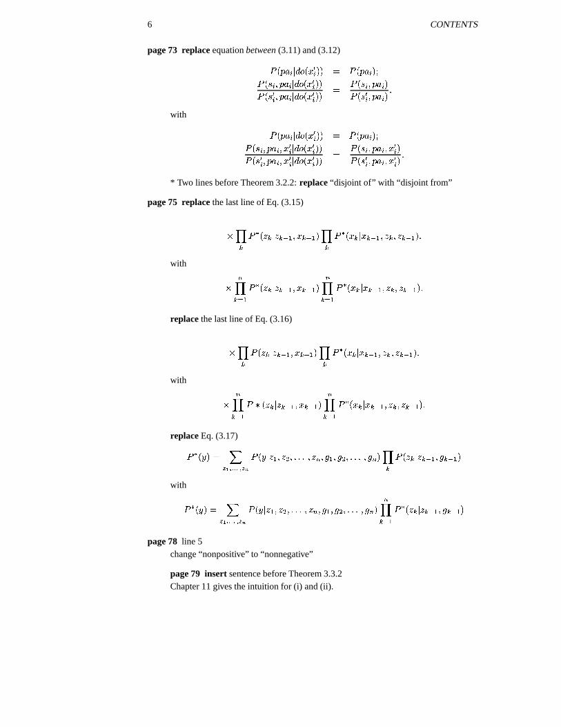
page 73 replace equation between (3.11) and (3.12)

� � � � � �� ' � � � � � �� 0�� ' � ��

� �� =with

� � � � � �� ' � � � � � �� 0�� ' � �� 0��

� �� =* Two lines before Theorem 3.2.2: replace “disjoint of” with “disjoint from”

page 75 replace the last line of Eq. (3.15)

�� : � � � : � �

�� : �� : � =

with

� >�� : �� : � � � : � >�

�� : �� : �� : � =replace the last line of Eq. (3.16)

�� : � �� : � �

�� : �� : �.=

with

� >�� : �� : � � � : � >�

�� : �� : �� : � =replace Eq. (3.17)

� � � 9 �(' )�� $��2$ �� 9 �[: �� < ,=�=�= �� > �� : ��< ,=�=�= ��> � �

�� : �� : �

with

�� 9 �(' )�� $��2$ �� 9 ��: � < �=,=�= �&> �� : ��< �=,=�= ��> � >�

�� : �� : �� : �page 78 line 5

change “nonpositive” to “nonnegative”

page 79 insert sentence before Theorem 3.3.2Chapter 11 gives the intuition for (i) and (ii).

CONTENTS 7

page 82 replace at line 2 of paragraph 2: “since there is no back-door path from � to � ,we simply have”with“since there is no unblocked back-door path from � to � in Figure 3.5, we simplyhave”

replace in Definition 3.3.3 (Front-Door): “(ii) there is no back-door path from � to� ; and”with“(ii) there is no unblocked back-door path from � to � ; and”

page 86 paragraph after Corollary 3.4.2replaceWhether Rules 1–3 are sufficient for deriving all identifiable causal effects remainsan open question. However, the task of finding a sequence of transformations (if suchexists) for reducing an arbitrary causal effect expression can be systematized and ex-ecuted by efficient algorithms (Galles and Pearl 1995; Pearl and Robins 1995), tobe discussed in Chapter 4. As we illustrate in Section 3.4.3, symbolic derivationsusing the hat notation are much more convenient than algebraic derivations that aimat eliminating latent variables from standard probability expressions (as in Section3.3.2, equation(3.24)). WithRules 1–3 have been shown to be complete, namely, sufficient for deriving all identi-fiable causal effects (Shpitser and Pearl 2006a; Huang and Valtorta 2006). Moreover,as illustrated in Section 3.4.3, symbolic derivations using the hat notation are moreconvenient than algebraic derivations that aim at eliminating latent variables fromstandard probability expressions (as in Section 3.3.2, equation(3.24)). However, thetask of deciding whether a sequence of rules exists for reducing an arbitrary causaleffect expression has not been systematized, and direct graphical criteria for identifi-cation are therefore more desirable. These will be developed in Chapter 4.

page 99 line 2 of 2nd paragraphreplace “in the counterfactual versus structural” with “in the potential-outcome ver-sus structural”

line 8-9 after Eq. (3.52)*replace “follow as theorems from the structural interpretation.” with “follow astheorems from the structural interpretation, and no other constraint need ever beconsidered.”

page 103 replace last paragraph on page (including footnote 15) with:To place this result in the context of our analysis in this chapter, we need to focusattention on condition (3.62) which facilitated Robins’ derivation of (3.63) and askwhether this formal counterfactual independency can be given a meaningful graphi-cal interpretation. The answer will be given in Chapter 4 (Theorem 4.4.1), where wederive a graphical condition for identifying the effect of a plan, i.e., a sequential setof actions. The condition reads as follows: � � 9 � ' �� is identifiable and is given

8 CONTENTS

by (3.63) if every action-avoiding back-door path from � � to � is blocked by somesubset � � of non-descendants of � � . (By “action-avoiding” we mean a path con-taining no arrow entering an � variable later than � � .) Chapter 11 (Section 11.4.2)further shows that the graphical criterion above is more general than that given in(3.62).

page 104 replace 1st paragraph withThe structural analysis introduced in this chapter supports and generalizes Robins’sresult from a new theoretical perspective. First, on the technical front, this analy-sis offers systematic ways of managing models where Robins’s starting assumption(3.62) is inapplicable. Examples are Figures 3.8(d)–(g)).

Second, on the conceptual front, the structural framework represents a fundamen-tal shift from the vocabulary of counterfactual independencies, to the vocabulary ofprocesses and mechanisms, in which human knowledge resides. The former requireshuman assessments of esoteric relationships such as (3.62), while the latter expressesthose same relationships in vivid graphical terms of missing links. Still, Robins’s pi-oneering research has proven (i) that algebraic methods can handle causal analysisin complex multistage problems and (ii) that causal effects in such problems can bereduced to estimable quantities (see also Sections 3.6.1 and 4.4).

page 105 add new section after end of Postscript

Postscript to 2nd Edition

Complete identification results

A key identification condition, which generalizes all the criteria established in thischapter has been derived by Jin Tian. It reads:

Theorem 3.6.1 (Tian and Pearl, 2002)A sufficient condition for identifying the causal effect � � 9 �� is that there existsno bi-directed path (i.e., a path composed entirely of bi-directed arcs) between �and any of its children.15

Remarkably, the theorem asserts that, as long as every child of � (on the pathwaysto � ) is not reachable from � via a bi-directed path, then, regardless of how com-plicated the graph, the causal effect � � 9 �� is identifiable. All identificationcriteria discussed in this chapter are special cases of the one defined in this theorem.For example, in Figure 3.5 � � 9 �� can be identified because the one path from� to � (the only child of � ) is not bi-directed. In Figure 3.7, on the other hand, thereis a path from � to �F: traversing only bi-directed arcs, thus violating the conditionof Theorem 3.6.1, and � ��9 �� is not identifiable.

15Before applying this criterion, one may delete from the causal graph all nodes that are not ancestors ofD

.

CONTENTS 9

Note that all graphs in Figure 3.8 and none of those in Figure 3.9 satisfy the condi-tion above. Tian and Pearl � 2002 � further showed that the condition is both sufficientand necessary for the identification of � �� , where � includes all variablesexcept � . A necessary and sufficient condition for identifying � � � �� , with�

and � two arbitrary sets, was established by Shpitser and Pearl (2006b). Sub-sequently, a complete graphical criterion was established for determining the identi-fiability of conditional interventional distributions, namely, expressions of the type� ��9 �� where � , � and � are arbitrary sets of variables (Shpitser and Pearl2006a).

These results constitute a complete characterization of causal effects in graphicalmodels. They provide us with polynomial time algorithms for determining whetheran arbitrary quantity invoking the �� operator is identified in a given semi-Markovian model and, if so, what the estimand is of that quantity. Remarkably,one corollary of these results also states that the �� -calculus is complete, namely, aquantity � ' � ��9 �� is identified if and only if it can be reduced to a �� -freeexpression using the three rules of Theorem 3.4.1.16

Applications and Critics

Gentle introductions to the concepts developed in this chapter are given in (Pearl2003) and (Pearl 2008a). Applications of causal graphs in epidemiology are reportedin Robins (2001), Hernan et al. (2002), Hernan et al. (2004), Greenland and Brum-back (2002), Greenland et al. (1999) Kaufman et al. (2005), Petersen et al. (2006),and VanderWeele and Robins (2007).

Interesting applications of the front door criterion (Section 3.3.2) were noted in socialscience (Morgan and Winship 2007) and economics (Chalak and White 2006).

Advocates of the “potential outcome” approach have been most resistant to accept-ing graphs or structural equations as the basis for causal analysis and, lacking theseconceptual tools, were led to dismiss important scientific concepts as “ill-defined”and “deceptive” (Holland 2001, Rubin 2004, Rubin 2005). Lauritzen (2004) andHeckman(2005) have criticized this attitude.

Equally puzzling are concerns of some philosophers (Cartwright 2007, Woodward2003) and economists (Heckman 2005) that the �� -operator is too local to modelcomplex, real life policy interventions, which sometimes affect several mechanismsat once and often involve conditional decisions, imperfect control, and multiple ac-tions. These concerns emerge from conflating the mathematical definition of a rela-tionship (e.g., causal effect) with the technical feasibility of testing that relationshipin the physical world. While the �� -operator is indeed an ideal mathematical tool(not unlike the derivative in differential calculus), it nevertheless permits us to spec-ify and analyze interventional strategies of great complexities. Readers will find

16This was independently established by Huang and Valtorta (2006).

10 CONTENTS

examples of such strategies in Chapter 4, and a further discussion of this issue inChapter 11 (Sections 11.4.3–11.4.7 and Section 11.5.4).

Chapter 4

page 108 paragraph 3, line 1replace “Traditional decision theory” with “Commonsensical decision theory”

page 109 2nd paragraph, 2nd line of mnemonic rhymesreplaceOn facts that preceded the act,WithOn what could have caused the act,

page 111 replace footnote 4:� The ID literature’s insistence on divorcing the links in the ID from any causal in-terpretation (Howard and Matheson 1981; Howard 1990) is at odds with prevailingpractice. The causal interpretation is what allows us to treat decision variables asroot nodes, unassociated with all other nodes (except their descendants). with� The ID literature’s insistence on divorcing the links in the ID from any causal in-terpretation (Howard and Matheson 1981; Howard 1990) is at odds with prevailingpractice. The causal interpretation is what allows us to treat decision variables asroot nodes and construct the proper decision trees for analysis; see Section 11.6 fora demonstration.

page 113 line 3replace “Section 1.1.4” with “Section 1.4.4”

page 114 Section 4.3.1, 1st paragraphreplaceTheorem 4.3.1 characterizes the class of “ �� -identifiable” models in the form of fourgraphical conditions, anyone of which is sufficient for the identification of � � 9 ��when � and � are singleton nodes in the graph. Theorem 4.3.2 then asserts thecompleteness (or necessity) of these four conditions; one of which must hold in themodel for � ��9 �� to be identifiable in �� -calculus. Whether these four conditions arenecessary in general (in accordance with the semantics of Definition 3.2.4) dependson whether the inference rules of �� -calculus are complete. This question, to the bestof my knowledge, is still open.WithTheorem 4.3.1 characterizes a class of “ �� -identifiable” models in the form of fourgraphical conditions, anyone of which is sufficient for the identification of � � 9 ��when � and � are singleton nodes in the graph. Theorem 4.3.2 then states the atleast one of these four conditions must hold in the model for � ��9 �� to be identifiablein �� -calculus. In view of the completeness of �� -calculus, we conclude that one of

CONTENTS 11

the four conditions is necessary for any method of identification compatible with thesemantics of Definition 3.2.4).

page 114 Section 4.3, last sentence before Section 4.3.1replaceIn this section we establish a complete characterization of the class of models inwhich the causal effect � ��9 �� is identifiable in �� -calculus.WithIn this section we characterize a simple class of models in which the causal effect� ��9 �� is identifiable in �� -calculus. This class is subsumed by the one establishedby Tian and Pearl (2002) in Theorem 3.7 and the complete characterization givenlater in Shpitser and Pearl (2006b). It is brought here for historical purposes only.

page 118 line 1replace � �Q'��4� �N� � �� with � �A'��4� �N� � ��

page 121 paragraph 4, line 1replace “Theorems 4.41 and” with “Theorems 4.4.1 and”

page 129 add to end of footnote 8“Cole and Hernan (2002) present examples in epidemiology.”

page 130-131 Section 4.5.4, replace entire sectionreplace entire section with:

4.5.4 Average Direct and Indirect Effects

Readers versed in structural equation models (SEMs) will note that, in linear systems,the direct effect � �� is fully specified by the path coefficient attached tothe link from � to � ; therefore, the direct effect is independent of the values �� at which we hold the other parents of � . In nonlinear systems, those values would,in general, modify the effect of � on � and thus should be chosen carefully torepresent the target policy under analysis. For example, the direct effect of a pillon thrombosis would most likely be different for pregnant and nonpregnant women.Epidemiologists call such differences “effect modification” and insist on separatelyreporting the effect in each subpopulation.

Although the direct effect is sensitive to the levels at which we hold the parents of theoutcome variable, it is sometimes meaningful to average the direct effect over thoselevels. For example, if we wish to assess the degree of discrimination in a givenschool without reference to specific departments, we should replace the controlleddifference

� �� ,�� L�N �� with some average of this difference over all departments. This average should mea-sure the increase in admission rate in a hypothetical experiment in which we instruct

12 CONTENTS

all female candidates to retain their department preferences but change their genderidentification (on the application form) from female to male.

Conceptually, we can define the average direct effect� � "�$ ",% �� as the expected

change in � induced by changing � from � to � � while keeping the other parentsof � constant at whatever value they would have obtained under �� . This hypo-thetical change, which Robins and Greenland (1991) called “pure” and Pearl (2001)called “natural,” is precisely what law makers instruct us to consider in race or sexdiscrimination cases: “The central question in any employment-discrimination caseis whether the employer would have taken the same action had the employee beenof a different race (age, sex, religion, national origin etc.) and everything else hadbeen the same.” (In Carson versus Bethlehem Steel Corp., 70 FEP Cases 921, 7thCir. (1996)).

Using the parenthetical notation of Eq. 3.51, the formal expression for the “naturaldirect effect,” reads:

� � "�$ "&% � � � ' � 3 � � �� 87 (4.11)

Here, � represents all parents of � excluding � , and the expression � �� represents the value that � would attain under the operation of setting � to � � and,simultaneously, setting � to whatever value it would have obtained under the setting� ' � . We see that

� � "�$ "&% � � � , the average direct effect of the transition from� to � � , involves probabilities of nested counterfactuals and cannot be written interms of the �� operator. Therefore, the average direct effect cannot in generalbe identified, even with the help of ideal, controlled experiments (see Robins andGreenland (1992) and Section 7.1 for intuitive explanation). Pearl (2001) have shownnevertheless that, if certain assumptions of “no confounding” are deemed valid,17 theaverage direct effect can be reduced to

� � "�$ ",% � � �(' )� 3 � � � �� 6� � � � �� 87 � �� (4.12)

The intuition is simple; the natural direct effect is the weighted average of controlleddirect effects, using the causal effect � �� as a weighing function. Under suchassumptions, the techniques developed in Section 4.4 for identifying control-specificplans, � � 9 �� : �� < �=�=,= �� > � , become applicable.

In particular, expression (4.12) is both valid and identifiable in Markovian models,where it can be written (using Corollary 3.2.6)

� � "�$ ",% � � �(' )� 3 � � � � � �� 87 )

�� ' � � (4.13)

17One sufficient condition is that R C Y E ]`] D C Y Z�� a E�� holds for some set�

of measured covariates. Seedetails and graphical criteria in (Pearl 2001) and in Petersen et al. (2006).

CONTENTS 13

4.5.5 Indirect Effects

Remarkably, the definition of the natural direct effect (4.11) can easily be turnedaround and provide an operational definition for the indirect effect – a conceptshrouded in mystery and controversy, because it is impossible, using the �� op-erator, to disable the direct link from � to � so as to let � influence � solely viaindirect paths.

The average indirect effect, IE, of the transition from � to � � is defined as the expectedchange in � affected by holding � constant, at � ' � , and changing � to whatevervalue it would have attained had � been set to � ' � � . Using our counterfactualnotation, this reads (Pearl 2001):

� � "�$ ",% � � �4' � 3 � � �� 6� � � � �� 87which is almost identical to the direct effect (Eq. (4.11)) save for a minor reversal of� and �0� .Indeed, it can be shown that, in general, the total effect � � of a transition is equalto the difference between the direct effect of that transition and the indirect effect ofthe reverse transition. Formally,

� � "�$ ",% �� ' � � � �� ' � � "�$ ",% � � � � � � "&% $ " ��

In linear systems, where reversal of transitions amounts to negating the signs of theireffects, we have the standard additive formula

� � "�$ " % � � �(' ' � � "�$ " % � � �� "�$ " % ��

This provides a formal justification for the additive formula, since each term is basedon an independent operational definition.

Note that the indirect effect has clear policy making implications. For example: ina hiring discrimination environment, a policy maker may be interested in predictingthe gender mix in the work force if gender bias is eliminated and all applicants aretreated equally, say the same way that males are treated today. This quantity will begiven by the indirect effect of gender on hiring, mediates by factors such as educationand aptitude, which may be gender-dependent.

More generally, a policy maker may be interested in the effect of issuing a directiveto select set of subordinate employees, or in carefully controlling the routing of mes-sages in a network of interacting agents. Such applications call for the definition ofpath-specific effects, that is, the causal effect of � on � through a selected set ofpaths. A complete analysis for Markovian models is given in Avin et al. (2005).

Note that in all these cases, the policy intervention invokes the selection of signals tobe sensed, rather than variables to be fixed. Pearl (2001) suggested that this signal se-lection operation are more fundamental to the notion of causation than manipulation;the latter being but a crude imitation of the former, devised for measurements.

14 CONTENTS

It is remarkable that, under certain graphical conditions, counterfactual quantitieslike

� � and � � that could not be expressed in terms of �� operators, can nev-ertheless be reduced to counterfactual-free formulas involving �� operators. Inother words, quantities that at first glance appear void of empirical content, can beestimated from empirical studies involving experimental control. We shall see ad-ditional examples of this “magic of scientific analysis” in Chapters 7, 9, and 11. Itconstitutes an invincible argument in defense of counterfactual analysis, as expressedin (Pearl 2000) against the critical stance of Dawid (2000) and Geneletti (2007).

A general analysis of the conditions under which counterfactual quantities can bereduced to �� expressions is given in Shpitser and Pearl (2007).

Acknowledgment

Sections 4.3 and 4.4 are based, respectively, on collaborative works with DavidGalles and James Robins. My interest in path-specific effects was stimulated byJacques Hagenaars, who pointed out the importance of quantifying indirect effectsin social science (see Chapter 11).

Chapter 5

page 141 2nd paragraph, line 4insert “Edwards 2000; Cowell et al. 1999;” before “Whittaker 1990;”

page 147 line 3 of 1st paragraph (after Rule 2)replace “would render � and � ” with “would render � and � ”

page 171 add new section

Notes Added to Second Edition

5.5.1 An Econometric Awakening?

After decades of neglect of causal analysis in economics, a surge of interest seems tobe in progress. In a recent series of papers, Jim Heckman (2000, 2003, 2005, 2007(with Vytlacil)) has made great efforts to resurrect and reassert the Cowles Commis-sion interpretation of structural equation models, and to convince economists that re-cent advances in causal analysis are rooted in the ideas of Haavelmo (1943) Marschak(1950), Roy (1951) and Hurwicz (1962). Unfortunately, Heckman still does not of-fer econometricians clear answers to the questions posed in this chapter (pp. 133,170, 171, 215-217). In particular, unduly concerned with implementational issues,Heckman rejects Haavelmo’s “equation wipe-out” as a basis for defining counter-factuals and fails to provide econometricians with an alternative definition, namely,

CONTENTS 15

a procedure, like that of Eq. (3.51), for computing the counterfactual � �� in awell-posed economic model, with � and � two arbitrary variables in the models.(See Sections 11.5.4–5.) Such a definition is necessary for endowing the “potentialoutcome” approach with a formal semantics, based on SEM, and thus unifying thetwo econometric camps currently working in isolation.

Another sign of positive awakening comes from the social sciences, through thepublication of Morgan and Winship’s book “Counterfactual and Causal Inference”(2007) in which the causal reading of SEM is clearly reinstated.18

5.5.2 Identification in Linear Models

In a series of papers, Brito and Pearl (2002ab, 2006) have established graphical cri-teria that significantly expand the class of identifiable semi-Markovian linear modelsbeyond those discussed in this chapter. They first proved that identification is ensuredin all graphs that do not contain bow-arcs, that is, no error correlation is allowedbetween a cause and its direct effect, while no restrictions are imposed on errorsassociated with indirect causes (Brito and Pearl 2002b). Subsequently, generalizingthe concept of instrumental variables beyond the classical patterns of Figures 5.9 and5.11, they establish a general identification condition that is testable in polynomialtime and subsumes all conditions known in the literature.

5.5.3 Robustness of Causal Claims

Causal claims in SEM are established through a combination of data and the set ofcausal assumptions embodied in the model. For example, the claim that the causaleffect � �� in Fig. 5.9 is given by � �J'�� is based on the assump-tions: � � �� '�� and � � � �� P' � � � �� both are shown in thegraph. A claim is robust when it is insensitive to violations of some of the assump-tions in the model. For example, the claim above is insensitive to the assumption� � �� ('�� which is shown in the model.

When several distinct sets of assumptions give rise to � distinct estimands fora parameter � , that parameter is called � -identified; the higher the � , the morerobust are claims based on � , because equality among these estimands imposes� �� constraints on the covariance matrix which, if satisfied in the data, indicatean agreement among � distinct sets of assumptions, thus supporting their valid-ity. A typical example emerges when several (independent) instrumental variablesare available � : � < ,=�=�= � � for a single link � � � , which yield the equalities� '�� '�� ' =�=,= '�� .Pearl (2004) gives a formal definition for this notion of robustness, and establishedgraphical conditions for quantifying the degree of robustness of a given causal claim.

18Though the SEM basis of counterfactuals is unfortunately not articulated.

16 CONTENTS

� -identification generalizes the notion of degree of freedom in standard SEM analy-sis; the latter characterizes the entire model, while the former applies to individualparameters and, more generally, to individual causal claims.

Chapter 6

page 174 replace in 4th line from end of page: “is not a statement about � being a positivecausal factor for � , properly written” with “is not a statement about � having apositive influence on � , properly written”

page 179 line 10replace “ � ' � � � �� example” with “ � '�� 0� � �

page 180 line 3 of footnote 6replace “[y]ou might” with “you might”

page 195 replace “Figure 6.1” with “Figure 6.3” in 5th line before end of 3rd paragraph

page 200 postscript added

Postscript to Chapter 6

Readers would be amused to learn that the first printing of this chapter did not stopstatisticians’ fascination with Simpson’s non-paradox. Textbooks continue to marvelat the phenomenon (Moore and McCabe 2005), and researchers continue to chase itsmathematical intricacies (Cox and Wermuth 2003) and visualizations (Rucker andSchumacher 2008) with the passion of the 1970-90’s, without once mentioning theword “cause” and without once stopping to ask: “What’s the point?” In contrast, myconfidence in the eventual triumph of the causal understanding of this non-paradoxhas been rekindled by a discussion published in the epidemiological literature, con-cluding in no ambiguous terms: “The explanations and solutions lie in causal rea-soning which relies on background knowledge, not statistical criteria” (Arah 2008).It appears that, as we enter the age of causation, we should look to epidemiologistsfor guidance and wisdom.

Chapter 7

page 206 4th line after Eq. (7.5)replace “(Dawid 1997).” with “(Dawid 2000).”

page 214–215 replace paragraph [through end of 7.1.4] with

The twin network reveals an interesting interpretation of counterfactuals of the form� *�+ � , where � is any variable and �� stands for the set of � ’s parents. Con-sider the question of whether � " is independent of some given set of variables in

CONTENTS 17

the model of Figure 7.3. The answer to this question depends on whether � � is� -separated from that set of variables. However, any variable that is � -separatedfrom � � would also be � -separated from � � , so the node representing � � can serveas a one-way proxy for the counterfactual variable � " . This is not a coincidence,considering that � is governed by the equation � '�� . By definition, theprobability of � " is equal to the probability of � under the condition where � isheld fixed at � . Under such condition, � may vary only if � � varies. Therefore, if� � obeys a certain independence relationship then � " (more generally, � *,+ � ) mustobey that relationship as well. We thus obtain a simple graphical representation forany counterfactual variable of the form � *,+ � . Using this representation, we can eas-ily verify from Figure 7.3 that �� and �� bothhold in the twin-network and, therefore,

� � � � � �� " � " � � H� � � �� " �� must hold in the model. Additional considerations involving twin networks, includ-ing generalizations to multi-networks (representing counterfactuals under differentanticedants) are reported in Shpitser and Pearl (2007).

page 217 4th line from top of pagereplace “observations � � ' � � � '�� ' � � . According to Definition” with“observations � � ' �� '�� ' � � (see Section 11.7.1.) According toDefinition”

page 220 2nd paragraph, line 7replace “including Dawid 1997)” with “including Dawid 2000)”

page 236 replace in 2nd line of footnote 17“Bonet (1999)” with “Bonet (2001)”

page 257 (no postscript added)

Chapter 8

page 264 replace footnote 3 with� Frangakis and Rubin (2002) dubbed them “Principal Stratification” and found themrather insightful. In the potential-outcome model (see Section 7.4.4), � stands foran experimental unit and � �� corresponds to the potential response of unit � totreatment � . The assumption that each unit (e.g., an individual subject) possessesan intrinsic, seemingly “fatalistic” response function has met with some objections(Dawid 2000), owing to the inherent unobservability of the many factors that mightgovern an individual response to treatment. The equivalence-class formulation of� �� mitigates those objections by showing that � �� evolves naturally and mathe-matically from any complex system of stochastic latent variables, provided only thatwe acknowledge their existence through the equation 9 '�� . Those who in-voke quantum-mechanical objections to the latter step as well (e.g. Salmon 1998),

18 CONTENTS

should regard the functional relationship 9 ' � �� as an abstract mathematicalconstruct, representing the extreme points (vertices) of the set of conditional proba-bilities � � 9 � � � satisfying the constraints of (8.1) and (8.2).

page 269 replace 4 lines before Eq. (8.19) to read:The analysis of

� �� reveals that, under conditions of no intrusion (i.e.,� �� : � � �4'�� , as in most clinical trials),

� �� can be identified precisely(Bloom 1984; Heckman and Robb 1986; Angrist and Imbens 1991). The naturalbounds governing

� �� in the general case can be obtained by similarmeans (Pearl 1995b), which yield

page 275 After Eq. (8.23), replaceHowever, the transition to a continuous � signals a drastic change in behavior, andit seems that the structure of Figure 8.1 induces no constraint whatsoever on theobserved density (Pearl 1995c).withHowever, the transition to a continuous � signals a drastic change in behavior, andled (Pearl 1995c) to conjecture that the structure of Figure 8.1 induces no constraintwhatsoever on the observed density. The conjecture was proven by (Bonet 2001).

page 280 Section 8.5.4, 2nd paragraph, 6th linereplacethe following four compliance-response populations: �� " ' � �� ' � � � � " '� ��'� � � " ' � ��P' � � � � " ' � ��P'� � � . Joe would have improved had hetaken cholestyramine if his response behavior is either helped ( � � ' � ) or always-recover ( �� '�� ).Withthe four compliance-response populations:

�� " '�� '�� " '�� ' � � � � " '�� ' �� " '�� ' � � � =Joe would have improved had he taken cholestyramine if and only if his responsebehavior is helped ( �� ' � ).


Chapter 9

page 297 2nd paragraph, 3rd linereplace “(Dawid 1997).” with “(Dawid 2000).”

page 298 after (9.38), within the next 5 lines, replace 9 ",% with 9��" % (4 places) and correctin last line of (9.39).replace

CONTENTS 19

In order to compute PNS, we must evaluate the probability of the joint event 9 " %�� 9 " .Given that these two events are jointly true only when � ' � �� , we have

�� ' � � 9 " 9 " % �' � � 9 " 9 " % �� 9 " �9 " % � � �� ' �

� � � ��(' � = ��= ��

WithIn order to compute PNS, we must evaluate the probability of the joint event 9;�" % � 9 " .Given that these two events are jointly true only when � ' � �� , we have

�� ' � � 9 " 9 �"&% �' � � 9 " 9 �" % �� 9 " �9 �" % � � �� ' �

�� (' � = ��= ��

page 302 Section 9.3.4, 2nd paragraph, line 11replace “(Dawid 1997);” with “(Dawid 2000);”


Chapter 10

page 329 add new postscript section

Postscript to Chapter 10Halpern and Pearl (2001ab) discovered a need to refine the causal beam definition of10.3.3. They retained the idea of defining actual causation by counterfactual depen-dency in a world perturbed by contingencies, but permitted a wider set of contingen-cies.

To see that the causal beam definition requires refinement, consider the followingexample.

Example 10.4.1 A vote takes place, involving two people. The measure � is passed

if at least one of them votes in favor. In fact, both of them vote in favor, and the

measure passes.

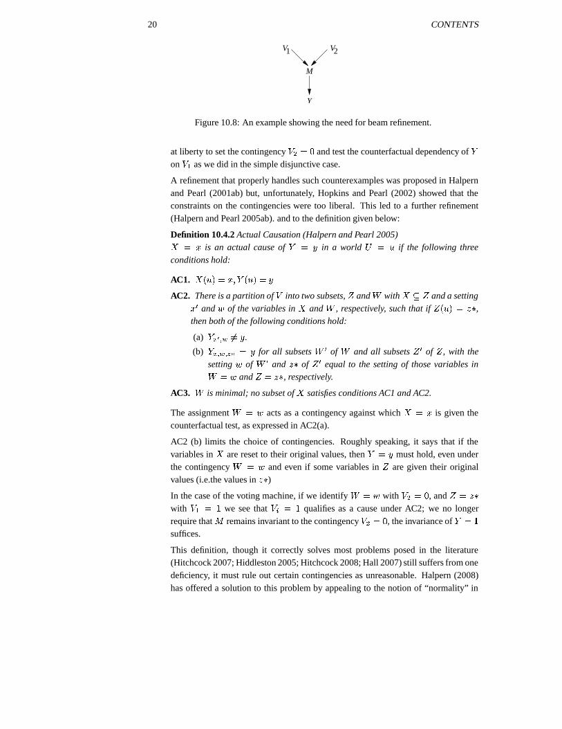
This version of the story is identical to the disjunctive scenario discussed in Section10.1.3, where we wish to proclaim each favorable vote, � : ' � and �0< ' � , acontributing cause of � ' � .However, suppose there is a voting machine that tabulates the votes. Let representthe total number of votes recorded by the machine. Clearly ' � : � � < and � '��iff � � . Figure 10.8 represents this more refined version of the story.

In this scenario, the beam criterion no longer qualifies � :Q' � as a contributing causeof � '�� , because �0< cannot be labeled “inactive” relative to , hence we are not

20 CONTENTS

VV

M

Y

1 2

Figure 10.8: An example showing the need for beam refinement.

at liberty to set the contingency �;< ' � and test the counterfactual dependency of �on �;: as we did in the simple disjunctive case.

A refinement that properly handles such counterexamples was proposed in Halpernand Pearl (2001ab) but, unfortunately, Hopkins and Pearl (2002) showed that theconstraints on the contingencies were too liberal. This led to a further refinement(Halpern and Pearl 2005ab). and to the definition given below:

Definition 10.4.2 Actual Causation (Halpern and Pearl 2005)� ' � is an actual cause of � ' 9 in a world � ' � if the following three

conditions hold:

AC1. � �� ' �� (' 9AC2. There is a partition of � into two subsets, � and

�with �� and a setting

�0� and � of the variables in � and�

, respectively, such that if � �� ' � ,then both of the following conditions hold:

(a) � "&%�$ �' 9 .

(b) � "�$ �$ � � ' 9 for all subsets� � of

�and all subsets � � of � , with the

setting � of� � and � of � � equal to the setting of those variables in� ' � and � ' � , respectively.

AC3.�

is minimal; no subset of � satisfies conditions AC1 and AC2.

The assignment� ' � acts as a contingency against which � ' � is given the

counterfactual test, as expressed in AC2(a).

AC2 (b) limits the choice of contingencies. Roughly speaking, it says that if thevariables in � are reset to their original values, then � ' 9 must hold, even underthe contingency

� ' � and even if some variables in � are given their originalvalues (i.e.the values in � )

In the case of the voting machine, if we identify� ' � with � <P' � , and � ' �

with �;: ' � we see that � � ' � qualifies as a cause under AC2; we no longerrequire that remains invariant to the contingency � < '�� , the invariance of � '��suffices.

This definition, though it correctly solves most problems posed in the literature(Hitchcock 2007; Hiddleston 2005; Hitchcock 2008; Hall 2007) still suffers from onedeficiency, it must rule out certain contingencies as unreasonable. Halpern (2008)has offered a solution to this problem by appealing to the notion of “normality” in

CONTENTS 21

default logic (Kraus et al. 1990; Spohn 1988; Pearl 1990b); only those contingenciesshould be considered which are at the same level of “normality” as their counterpartsin the actual world.

Epilogue

No changes.

Chapter 11

New chapter – separate file.

CONTENTS 1

NEW PRINTING CORRECTIONS/ADDITIONSTO BE IMPLEMENTED BY CAMBRIDGEIN THE SECOND EDITION OF CAUSALITY

Updated 8/20/08

Chapter 1

page 27 1st line after Eq. (1.40)replace “the set of variables judged to be immediate causes of � � ” with“the set of variables that directly determine the value of � � ”

page 27 3rd paragraphreplace paragraph starting “A set of equations...” (including footnote 13) with

The interpretation of the functional relationship in (1.40) is the standard interpreta-tion that functions carry in physics and the natural sciences; it is a recipe, a strategy,or a law specifying what value nature would assign to � � in response to every possi-ble value combination that �� might take on. A set of equations in the formof (1.40) and in which each equation represent an autonomous mechanism is calledstructural model; if each variable has a distinct equation in which it appears on theleft-hand side (called the dependent variable), then the model is called a structural

causal model or a causal model for short.13 Mathematically, the distinction be-tween structural and algebraic equations is that any subset of structural equations is,in itself, a valid structural model – one that represents conditions under some set ofinterventions.

Chapter 4

page 113 -5 lines from bottom of pageinsert after “hat-free expression.”Kuroki and Miyakawa (1999a, 2003) present graphical criteria.

page 126 line 2-3 after Figure 4.8replace“Kuroki and Miyakawa (1999).” withKuroki (with Miyakawa 1999ab, 2003; with et al. 2003; with Cai 2004).

page 129 line 3 after Figure 4.9replace “ � = applicant’s career objectives;” with“ � = applicant’s (pre-enrollment) career objectives;”

13Formal treatment of causal models, structural equations, and error terms are given in Chapter 5 (Section 5.4.1)and Chapter 7 (Sections 7.1 and 7.2.5).

2 CONTENTS

Chapter 6

page 194 -8 lines from bottom of pagereplace “(at each level of � ) and the association between � and � may vanish aswell.” with “(at each level of � ); similarly, the association between � and � mayvanish.”

page 194 -3 lines from bottom of pagereplace “is associated neither with the exposure � � � nor with the disease �� .” with“is not associated with the disease � � � .”

page 194-196 replace starting with last paragraph (last 2 lines) of page 194 through lastparagraph of 6.5.2 (on page 196):

The intuition behind Rothman and Greenland’s statement just quoted can be expli-cated formally through the notion of stability: a variable that is stably unassociatedwith either � or � can safely be excluded from adjustment. Alternatively, Rothmanand Greenland’s statement can be supported (without invoking stability) by using thenotion of nontrivial sufficient set (Section 3.3)—a set of variables for which adjust-ment will remove confounding bias. It can be shown (see the end of this section) thateach such set � , taken as a unit, must indeed be associated with � and be condition-ally associated with � , given � . Thus, Rothman and Greenland’s condition is validfor nontrivial sufficient (i.e., admissible) sets but not for the individual variables inthe set.

The practical ramifications of this condition are as follows. If we are given a set� of variables that is claimed to be sufficient (for removing bias by adjustment),then that claim can be given a necessary statistical test: � as a compound variablemust be associated both with � and with � (given � ). In Figure 6.5, for example,

� :�'�� and � < '�� are sufficient and nontrivial; both must satisfy thecondition stated.

Note that, although this test can be used for screening sets claimed to be sufficient,it does not constitute a test for detecting confounding. Even if we find a set � ina problem that is associated with both � and � , we are still unable to concludethat � and � are confounded. Our finding merely qualifies � as a candidate forsufficient status in case confounding exists, but we cannot rule out the possibilitythat the problem is unconfounded to start with. (The sets � ' � � � � or � '� � � in Figure 6.1 illustrate this point.) Observing a discrepancy between adjustedand unadjusted associations (between � and � ) does not help us either, because(recalling our discussion of collapsibility) we do not know which—the preadjustmentor postadjustment association—is unbiased (see Figure 6.4).

CONTENTS 3

Proof of Necessity

To prove that � � : � and �� < � must be violated whenever � stands for a nontrivial suf-ficient set � , consider the case where � has no effect on � . In this case, confoundingamounts to a nonvanishing association between � and � . A well-known property ofconditional independence, called contraction (Section 1.1.5), states that violation of�� : � , �� , together with sufficiency, �� , implies violation of nontriviality,�� :

�� 4=Likewise, another property of conditional independence, called intersection, statesthat violation of � � < � , � �� , together with sufficiency, �� , also impliesviolation of nontriviality, �� .

� � � � � � �� 4=Thus, both ��4: � and � �(< � must be violated by any nontrivial sufficient set � .

Note, however, that intersection holds only for strictly positive probability distribu-tions, which means that the Rothman-Greenland condition may be violated if deter-ministic relationships hold among some variables in a problem. This can be seenfrom a simple example in which both � and � stand in a one-to-one functional re-lationship to a third variable, � . Clearly, � is a nontrivial sufficient set yet is notassociated with � given � ; once we know the value of � , the probability of � isdetermined, and would no longer change with learning the value of � .

Chapter 11

Minor corrections made throughout Chapter 11, with exception to Section 11.3 which hasmajor revisions – see separate file.

CONTENTS 1

CORRECTIONS/ADDITIONSTO BE IMPLEMENTED BY CAMBRIDGEIN THE SECOND EDITION OF CAUSALITY PROOFS

Updated 11/4/08

Chapter 3

page 77 line 3 after Definition 3.2.3,replace “samples of � ” with “samples of � �� ”

Chapter 6

page 187 line -3 (before footnote 12)replace “of � and � is” with “of � and � � � � is”

page 195 -5 lines before “Proof of Necessity”replace “Figure 6.1” with “Figure 6.3”

Chapter 7

page 251 2nd paragraph, line 4replace “Section 7.1.2.” with “Section 7.2.2.”

Chapter 11

pages 333-4 replace paragraph starting “Divorcing simple concepts...” with

Divorcing simple concepts from the province of statistics - the most powerful formallanguage known to empirical scientists – can be traumatic indeed. Social scientistshave been laboring for half a century to evaluate public policies using statisticalanalysis, anchored in regression techniques, and only recently confessed, with greatdisappointment, what should have been recognized as obvious in the 1960’s: “Re-gression analysis typically do nothing more than produce from a data set a collectionof conditional means and conditional variances” (Berk 2004, p. 237). Economistshave gone through a similar trauma with the concept of exogeneity (Section 5.4.3).Even those who recognized that a strand of exogeneity (i.e., superexogeneity) isof a causal variety came back to define it in terms of distributions (Maddala 1992,Hendry 1995) – crossing the demarcation line was irresistible. And we understandwhy; defining concepts in term of prior and conditional distributions - the ultimateoracles of empirical knowledge - was considered a mark of scientific prudence. Weknow better now.

2 CONTENTS

page 340 insert 2 new paragraphs after line 2

It is also important to note that the danger of creating new bias by adjusting forwrong variables can threaten randomized trials as well. In such trials, investigatorsmay wish to adjust for covariates despite the fact that, asymptotically, randomizationneutralizes both measured and unmeasured confounders. Adjustment may be soughteither for improving precision (Cox 1958, pp. 48–55), or to match imbalanced sam-ples, or to obtain covariate-specific causal effects. Randomized trials are immuneto adjustment-induced bias when adjustment is restricted to pre-treatment covari-ates, but adjustment for post-treatment variables may induce bias by the mechanismshown in Figure 11.5 or, more severely, when correlation exists between the adjustedvariable � and some factor that affects outcome (e.g., � � in Figure 11.5).

As an example, suppose treatment has a side effect (e.g., headache) in patients thatare predisposed to disease � . If we wish to adjust for disposition and adjust insteadfor its proxy, headache, a bias would emerge through the spurious path: treatment� headache � predisposition � disease. However, if we are careful never to adjustfor any consequence of treatment (not only those that are on the causal pathway todisease), no bias will emerge in randomized trials.

page 342 replace footnote 4 with� In fact, in those cases where “strong ignorability” is used to guide the choice of � ,the guidelines issued are invariably wrong, perpetuating myths such as: “In princi-ple, there is little or no reason to avoid adjustment for a true covariate, a variabledescribing subjects before treatment.” (Rosenbaum 2002, p. 76) or “a confoundermust be associated with both treatment and disease,” or “strong ignorability requiresmeasurement of all covariates related to both treatment and outcome.”

page 342 2nd paragraph, last sentence:replace “(ch11-eq11x)” with “(11.4)”

page 342 5th paragraph, last sentence:replace “ � � �� from � ” with “

�from � ”

page 342 6th paragraph, 1st line:replace “designated � � � �� ” with “designated

�”

page 342 replace footnote 4 with� In fact, in the rare cases where “strong ignorability” is used to guide the choice ofcovariates, the guidelines issued are wrong or inaccurate, perpetuating myths suchas: “there is no reason to avoid adjustment for a variable describing subjects beforetreatment,” “a confounder is any variable associated with both treatment and dis-ease,” or “strong ignorability requires measurement of all covariates related to bothtreatment and outcome.”

page 343 replace Figure 11.7 figure with corrected figure file, “ch11-fig11y”(“ � � � �� ” is replaced with “

�”)

CONTENTS 3

page 343 Figure 11.7 caption, replace “ignor-ability” with “ignorability”

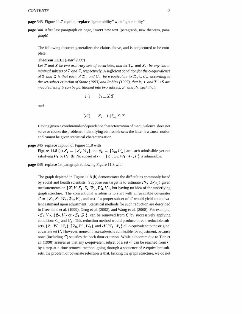
page 344 After last paragraph on page, insert new text (paragraph, new theorem, para-graph)

The following theorem generalizes the claims above, and is conjectured to be com-plete.

Theorem 11.3.1 (Pearl 2008)Let � and � be two arbitrary sets of covariates, and let �� and �� be any two � -minimal subsets of � and � , respectively. A sufficient condition for the � -equivalenceof � and � is that each of � � and � � be � -equivalent to � � � � � according to

the set-subset criterion of Stone (1993) and Robins (1997), that is, � and � � � are� -equivalent if � can be partitioned into two subsets, � : and � < , such that:

� � � � � : � � � �

and

� �� < � � � � : � �

Having given a conditional-independence characterization of � -equivalence, does notsolve or course the problem of identifying admissible sets; the latter is a causal notionand cannot be given statistical characterization.

page 345 replace caption of Figure 11.8 withFigure 11.8 (a) � : ' � � : � < � and � < ' � � < � : � are each admissible yet notsatisfying � : or � < . (b) No subset of � ' � � : � < � : � < � � is admissible.

page 345 replace 1st paragraph following Figure 11.8 with

The graph depicted in Figure 11.8 (b) demonstrates the difficulties commonly facedby social and health scientists. Suppose our target is to estimate � � 9 �� givenmeasurements on � � � �F: �(< � : � < � � , but having no idea of the underlyinggraph structure. The conventional wisdom is to start with all available covariates� ' � �4: �(< � : � < � � , and test if a proper subset of � would yield an equiva-lent estimand upon adjustment. Statistical methods for such reduction are describedin Greenland et al. (1999), Geng et al. (2002), and Wang et al. (2008). For example,� � : � � , � � < � � or � �4: �(< � , can be removed from � by successively applyingconditions � : and � < . This reduction method would produce three irreducible sub-sets, � � : � : � < � , � � < � : � < � , and � � � : � < � all � -equivalent to the originalcovariate set � . However, none of these subsets is admissible for adjustment, becausenone (including � ) satisfies the back door criterion. While a theorem due to Tian etal. (1998) assures us that any � -equivalent subset of a set � can be reached from �by a step-at-a-time removal method, going through a sequence of � -equivalent sub-sets, the problem of covariate selection is that, lacking the graph structure, we do not

4 CONTENTS

know which (if any) of the many subsets of � is admissible. The next subsection dis-cusses how external knowledge as well as more refined analysis of the data at hand,can be brought to bear on the problem.

page 346 replace 2nd paragraph with

For example, the model depicted in Figure 11.9 is observationally equivalent to thatof Figure 11.8 (b). In particular, it satisfies all the conditional independencies impliedby the latter, and none others. However, in contrast to Figure 11.8 (b), the sets� � : � : � < � � � � : � < � , and � � < � : � < � are admissible. Adjusting for thelatters would remove bias if the correct model is Figure 11.9 and would produce biasif the correct model is 11.8 (b).

page 346 replace caption of Figure 11.9 withFigure 11.9 A model that is statistically indistinguishable from that of Figure 11.8(b), in which the irreducible sets � �A: � : � < � , � � : � < � � , and � � : � < � < �are admissible.

page 349 in last paragraph of page 349, -3 line from footnote 9, replace “absolves onefrom” with “can cause no harm (Rosenbaum 2002, p. 76) or”

page 350 1st paragraph, replace last sentence with“Examples are abound (e.g., Figure 6.3) where adding a variable to the analysis, notonly is not needed but would introduce irreparable bias.”

page 360-1 Section 11.4.6, 1st paragraph, last sentence - replace with“In so doing, she unveils several areas in need of systematic clarifications; I willaddress them in turn.”

page 361 replace in last sentence of page:“Thus, Cartwright is mistaken in asserting that” with “Thus, it would be a mistake toassume that”

page 361 replace in last sentence of page:Claim (1) may apply in some cases, but certainly not in most;

page 362 replace line 3 of page with‘Claim (1) may apply in some cases, but certainly not in most; in many studies ourgoal is”

page 362 replace paragraph 6 with

Ironically, shunning mathematics based on ideal atomic intervention may condemnscientists to ineptness in handling realistic non-atomic interventions.

CONTENTS 5

References

page 438 In [Kuroki and Miyakawa, 2003] citation, change “Journal of the Japanese RoyalStatistical society” to “Journal of the Royal Statistical Society”

CONTENTS 1

CORRECTIONS/QUESTIONS FOR PROOFS OF THESECOND EDITION OF CAUSALITY (dated 11/13/08)

Updated 12/19/08 - still working on

Preface

page xviii stet original ending and add new heading (check copy edit format throughoutfor style/consistency)J.P.Los AngelesAugust 1999

Preface to Second Edition

per judea note - “if space permits [where?] - popular reception of the unifying theoryof Modifiable Structural Models (MSM) presented in this book call...”

Chapter 1

page 24 question: in (iii), should “ � ' �� ” be on previous line?

page 47 question: last sentence, 2nd paragraph. should it be “(i.e., polytrees)” not “apolytrees”?

Chapter 2

page 48 question: in paragraph following def 2.4.1, should it be “ � �� ” (cap � )?

page 64 question: what is the format of “Postscript” heading for the Second Edition?

Chapter 3

page 105 heading for 2nd edition postscript left off after line 2. check style.

page 105 in paragraph 4 of (missing) postscirpt heading, center the asterisk in �� page 106 insert comma between greenland:etal99 and kaufman:etal05 cites, “Greenland

et al. (1999), Kaufman et al. (2005)”

2 CONTENTS

Chapter 4

page 114 section 4.3, line 5: “ �� calculus” should be “ �� -calculus”

page 114 section 4.3.1, line 3: “then states the at least” should be “then states that at least”(the should be that)

page 114 section 4.3.1, line 4: “ �� calculus” should be “ �� -calculus”

page 114 section 4.3.1, line 5: “ �� calculus” should be “ �� -calculus”

page 131 section 4.5, footnote 9: replace “(Pearl 2001)” with “Pearl (2001)”

page 132 completely replace section 4.5.5 (reduced to fit page length limitaion)

Chapter 5

page 135 pages from hereon are -2 and revert back to original page numbering

page 173 (171) missing “Notes Added to Second Edition” heading before section 5.5.1

Chapter 6

page 197 (195) correct both formulas on bottom of page:1st should be �� ... (

�, not )

2nd should be � �� ... (�

, not )

Chapter 7

page 202 (200) replace “Postscript” heading with “Postscript to Second Edition”

page 219 (217) line 4, replace “Section 11.7.1.)” with “Section 11.7.1).”

Chapter 8 & 9

no corrections.

Chapter 10

page 331 (329) replace “Postscript” heading with “Postscript to Second Edition”

CONTENTS 3

Chapter 11

page 347 (345) question: -2 from bottom, should it be “solve or cause the problem” no“solve or course”?????

page 348 (346) question: in 1st paragraph, lines 11 and 15, change “is” to “are”?????

page 352 (350) correction: 2nd paragraph, line 5: replace “or the need to reason” with“and can absolve one from thinking”

page 352 (350) in footnote 9:replace “(e.g., Rubin 2004).” with “(e.g., Rubin 2004, 2008).”

ADDITIONS TO SUBJECT INDEXTO BE IMPLEMENTED BY CAMBRIDGEIN THE SECOND EDITION OF CAUSALITY PROOFS

Updated 11/26/08

final page numbers to be double-checked

ADD TO SUBJECT INDEX

Action-avoiding, p. 103

Assumptions, p. 40

Bi-directed, p. 105

Causal beam, p. 329

Causal model, p. 27

$c$-equivalence, p. 344

Completeness, p. 68, 105

Convolution, p. 64

Counterfactuals - nested, p. 130ish

Cowles Commission, p. 171

Default logic, p. 330ish

Degree of freedom, p. 171

Direct, p. 130

Direction, p. 43

Discovery, p. 64

Distiction between statistical and causal, p. 40

Equivalence-class, p. 264

Exogeneity, p. 333

Identification, p. 105

Ignorability, p. 342

4 CONTENTS

Indirect, p. 130

Indirect effects, p. 131ish

Instrumental variables, p. 171

Myths, p. 342

Nature, p. 27

Nontrivial sufficient set, p. 194ish

Recovery, p. 43

Path-specific effects, p. 131ish

Potential-outcome, p. 68

Principal Stratification, p. 264

Randomized trials, p. 340

Regression, p. 333

Robustness, p. 171

Sex discrimination..., add p. 131

Shocks, p. 64

Simpson’s non-paradox, p. 200

Strong ignorability, p. 342

Superexogeneity, p. 333

Syntax, p. 40

Thermodynamics, p. 43

Twin network, p. 214

ADD TO AUTHOR INDEX

Angrist, p. 269

Arah, p. 200

Avin, p. 131ish (add etal names)

Berk, p. 333

Bessler, p. 64

Bloom, p. 269

Bonet, p. 275

Brito, p. 171

Brumback, p. 105

Cartwright, p. 105

Chalak, p. 105

Cole, p. 129

Cox, p. 40, 200, 340

Dawid, p. 34, 131ish, 264

Demiralp, p. 64

Frangakis, p. 264

Galles, p. 131ish

Geiger, p. 11

Geng, p. 345 (add etal names)

CONTENTS 5

Glymour, p. 64

Gopnik, p. 64 (add etal names)

Granger, p. 64

Greenland, p. 105 (add etal names), 130ish, 194ish, 345 (etal)

Haavelmo, p. 171

Hall, p. 330ish

Halpern, p. 329, 330ish

Heckman, p. 105, 171, 269

Hendry, p. 333

Hernan, p. 105 (add etal names), 129

Hiddleston, p. 330ish

Hitchcock, p. 330ish

Holland, p. 105

Hoover, p. 64

Hopkins, p. 330ish

Howard, p. 111

Hoyer, p. 64 (add etal names)

Huang, p. 86, 105

Hurwicz, p. 171

Imbens, p. 269

Kaufmann, p. 105 (add etal names)

Kraus, p. 330ish (add etal names)

Lauritzen, p. 105

Maddala, p. 333

Marshak, p. 171

Matheson, p. 111?

McCabe, p. 200

Moneta, p. 64

Moore, p. 200

Morgan, p. 105, 171

Pearl, p. 11, 40, 41, 43, 64, 86, 105, 114, 130ish, 131ish, 171, 215ish, 269, 275, 329, 330ish, 344

Petersen, p. 105 (add etal names), 130ish (add etal names)

Rebane, p. 41, 43

Reichenbach, p. 43

Robb, p. 269

Robins, p. 64 (add etal names), 105, 130ish, 131ish, 344

Rosenbaum, p. 342, 349

Rothman, p. 194ish

Roy, p. 171

Rubin, p. 105, 264, 352

Rucker, p. 200

Salmon, p. 264

Scheines, p. 64

6 CONTENTS

Schumacher, p. 200

Shimizu , p. 64 (add etal names)

Shpitser, p. 86, 105, 114, 131ish, 215ish

Spirtes, p. 64 (add etal names)

Spohn, p. 330ish

Stone, p. 344

Swanson, p. 64

Tian, p. 64, 105, 114, 345 (etal)

Valtorta, p. 86, 105?

VanderWeele, p. 105

Vytlacil, p. 171

Wang, p. 345 (add etal names)

Wermuth, p. 40, 200

White, p. 105

Winship, p. 105, 171

Woodward, p. 105

CONTENTS 1

COPYEDIT INSERTS FOR PROOFS OF THE SECONDEDITION OF CAUSALITY (Updated 1/9/08)

insert-43 (sent to cup but not implemented): Such thought experiments tell us that cer-tain patterns of dependency, void of temporal information, are conceptually charac-teristic of certain causal directionalities and not others. Reichenbach (1956) who wasthe first to wonder about the origin of those patterns suggested that they are charac-teristic of Nature, reflective of the second law of thermodynamics. Rebane and Pearl(1987) posed the question in reverse, and asked whether the distinctions among thedependencies associated with the three basic causal substructures: � � � � � ,� � � � � and � � � � � can be used to uncover genuine causal in-fluences in the underlying data generating process. They quickly realized that thekey to determining the direction of the causal relationship between � and � lies in“the presence of a third variable � that correlates with � but not with � ,” as in thecollider � � � � � , and developed an algorithm that recovers both the edgesand directionalities in the class of causal graphs that they considered (i.e., polytrees).

The investigation in this chapter formalizes these intuitions and extends the Rebane-Pearl recovery algorithm to general graphs, including graphs with unobserved vari-ables.

insert-60: Rephrased as a logical guarantee, we can categorically assert that the IC* algo-rithm will never label an arrow � � � as genuine if in fact � has no causal influenceon � and if the observed distribution is stable relative to its underlying causal model.

insert-61: and this is indeed what scientists attempt to accomplish through controlled ex-perimentation. Absent such experimentation, the best one can do is to rely on virtualcontrol variables, like those revealed by Nature through the dependence patterns ofDefinitions 2.7.1–2.7.4.

insert-63: It is people’s quest for stability that explains why they find it impossible to ex-emplify intransitive patterns of dependencies except by envisioning a common effectof two independent causes (see page 43). Any story that convincingly exemplifies agiven pattern of dependencies must sustain that pattern regardless of the numericalvalues of the story parameters – a requirement we called “stability.”

insert-64 (new paragraph): A program of benchmarks of causal discovery algorithms,named “Causality Workbench,” has been reported by Guyon et al. (2008ab;http://clopinet.com/causality). Regular contests are organized in which participantsare given real data or data generated by a concealed causal model, and the challengeis to predict the outcome of select set of interventions.

insert-70: Balke and Pearl (1994ab) proposed it as the basis for defining counterfactuals,see (3.51).

2 CONTENTS

insert-73 (not implemented per 3/13/07): Replace equation between (3.11) and (3.12)with:

� � � � � �� ' � � � � � �� 0�� ' � �� 0��

� �� =insert-79 (2nd line from top): [recasts the confounding problem in counterfactual vocab-

ulary but falls short of providing] researchers with a workable criterion to guide thechoice of covariates (see Section 11.3.2).

insert-98a: ... mathematical equivalence] – a theorem in one entails a theorem in the other.In this section we highlight the key methodological differences.

insert-98b: ; but lacking formal semantics, e.g., (3.51), did not progress beyond the stageof a “framework.”

insert-104: Robins’s pioneering research has shown that, to properly manage multistageproblems with time-varying treatments, the opaque condition of “ignorability” (3.53)should be broken down to its sequential constituents. This has led to the sequentialback-door criterion of (Theorem 4.4.5).

insert-106: [lacking these conceptual tools,] were unable to address the issue of covariateselection (Rosenbaum 2002, p. 76; Rubin 2007, 2008a) and were led to [dismiss thisand other scientific questions as “ill-defined”..]

insert-106b (bold subtitle):

Chapter road map to the main results

The three key results in this chapter are: 1. The control of confounding, 2. Theevaluation of policies, and 3. The evaluation of counterfactuals.

1. The problem of controlling confounding bias is resolved through the back-doorcondition (Theorem 3.3.2, pp. 79-80) – a criterion for selecting a set of covari-ates that, if adjusted for, would yield an unbiased estimate of causal effects.

2. The policy evaluation problem – to predict the effect of interventions from non-experimental data – is resolved through the �� -calculus (Theorem 3.4.1, pp.85-86) and the graphical criteria that it entails (Theorem 3.3.4, p. 83; Theorem3.6.1, p. 105). The completeness of �� -calculus implies that any (nonparamet-ric) policy evaluation problem that is not supported by an identifying graph, oran equivalent set of causal assumptions, can be proven “unsolvable.”

3. Finally, equation (3.51) provides a formal semantics for counterfactuals,through which probabilities of of counterfactuals can be defined and evaluatedin the framework of scientific theories (see Chapter 7).

CONTENTS 3

insert-114a: In this section we characterize a wider class of models in which the causaleffect � � 9 �� is identifiable. This class is subsumed by the one established by Tianand Pearl (2002a) in Theorem 3.7 and the complete characterization given later inShpitser and Pearl (2006b). It is brought here for its intuitive appeal.

insert-114b: Theorem 4.3.1 characterizes a class of models in the form of four graphicalconditions, anyone of which is sufficient for the identification of � � 9 �� when �and � are singleton nodes in the graph. Theorem 4.3.2 then states the at least oneof these four conditions must hold in the model for � � 9 �� to be identifiable in �� -calculus. In view of the completeness of �� calculus, we conclude that one of thefour conditions is necessary for any method of identification compatible with thesemantics of Definition 3.2.4).

insert-118: Although the completeness results of Shpitser and Pearl (2006a) now offer aprecise characterization of the boundary between the identifying and non-identifyingmodels (see discussion following Theorem 3.6.1), the conditions of Theorem 4.3.2may still be useful on account of their simplicity and intuitive appeal.

insert-123: Note that admissibility (4.5) requires that each subsequence� : ,=L=�= �� : �4: �=�=�= � � blocks every “action-avoiding” back-door path from� � to � (see page 103).

insert-165: The manipulative account that we have invoked in defining the empirical con-tent of structural equations (Definition 5.4.1) is adequate in linear systems, wheremost causal quantities of interest can be inferred from experimental studies at thepopulation level (see Section 11.7.1). In nonlinear and nonparametric models, weoccasionally need to go down to the individual unit level and invoke the (more fun-damental) counterfactual reading of structural equations, as articulated in equation(3.51) and footnote 17, page 162. The analysis of indirect effects is a case in point;its definition (4.14) rests on nested counterfactuals and cannot be expressed in termsof population averages. Such analysis is necessary to give indirect effects operationalmeaning, independent of total and direct effects (see Section 11.4.2). With the help ofcounterfactual language, however, we can give indirect effects a simple operationaldefinition: The indirect effect of � on � is the increase we would see in � whileholding � constant and increasing � to whatever value � would have attained undera unit increase of � (see Section 4.5.5 for a formal definition). In linear systems, thisdefinition coincides, indeed, with the difference between the total and direct effects.See chapter 11 for further discussion on the role of indirect effects in social scienceand policy analysis (Pearl 2005a).

insert-170: Some of these confusions are reflected in the many questions that I have re-ceived from readers (Section 11.5), to whom I dedicated a “SEM Survival Kit” (Sec-tion 11.5.3) – a set of arguments for defending the causal reading of SEM and itsscientific rationale.

4 CONTENTS

insert-195: Note however that, although this test can screen out some obviously bad sets� claimed to be sufficient, it has nothing to do with sufficiency or confounding; itmerely tests for nontriviality, i.e., that adjusting for � would change the associationbetween � and � . When we find a nontrivial set � , we still cannot be sure whetherthe association was unbiased to start with (as in Figure 6.1) or that it turned unbiasedafter the adjustment.

insert-200: A notable exception is Larry Wasserman’s All Of Statistics (Wasserman 2004)the first statistics textbook to treat Simpson’s reversal in its correct causal context.

insert-203: (iii) � is a set of functions �� : � < �=�=,= � > � such that each � � is a mappingfrom (the respective domains of) � � � �� to � � , where � � � � and �� and the entire set � forms a mapping from � to � . In other words, each� � in

� � ' � � � �� ' � ,=�=,= �� assigns a value to � � that depends on (the values of) a select set of variables in� � � , and the entire set � has a unique solution � �� .3 4

insert-204 (for clarity of handwritten edit): Let � and � be two subsets of variables in� . The counterfactual sentence “ � would be 9 (in situation � ), had � been � ” isinterpreted as the equality � " ��F' 9 , with � " �� being the potential response of �to � ' � .

insert-206 (for clarity of handwritten edit): The definition of � " and �P�" in terms of thesolution for � in two distinct submodels, governed by a standard probability spaceover � , neutralizes these objections by interpreting the contradictory joint statementas an ordinary event in � -space.

insert-226: If � is the set of variables directly constrained by �� , we can ask whetherthere is one member of � , say � � that accounts for the changes in all the othersolutions. If the identity of that predictive member remains the same for all choicesof � � and � , then we designate � � as the dependent variable in � � .

insert-243: In contrast to the structural modeling, however, this variable is not derivedfrom a causal model or from any formal representation of scientific knowledge, butis taken as a primitive—that is, an unobserved variable that reveals its value onlywhen � coincides with the treatment actually received, as dictated by the consistencyrule � ' � � � " ' � (equation (7.20)). Consequently, the potential-outcomeframework does not provide a mathematical model from which such rules could bederived or on the basis of which an axiomatic characterization could be attempted todecide, for example, whether additional rules should be deployed, or whether a givencollection of potential-outcome expressions is redundant or contradictory.

3The choice of �� (connoting parents) is not arbitrary, but expresses the modeller’s understanding of whichvariables Nature must consult before deciding the value of � .

4Uniqueness is ensured in recursive (i.e., acyclic) systems. Halpern (1998) allows multiple solutions in non-recursive systems.

CONTENTS 5

insert-244a: and became a mathematical fact through the explicit translation of equation(3.51) followed by the completeness result of Theorem 7.3.6.

insert-244b: Indeed, researchers who shun structural equations or graphs tend to avoidsubject matter knowledge in their analyses.

insert-251: satisfy the back-door condition, because the inequality in Definition 7.5.1 canalways be satisfied by conditioning on some imagined factor � (as in Figure 6.2 (c))that generates spurious associations between � and � . nd became a mathematicalfact through the explicit translation of equation (3.51) followed by the completenessresult of Theorem 7.3.6.

insert-259 (clarifying end of Preface): and (iii) that prior knowledge can be harnessedeffectively to obtain Bayesian estimates of those impacts.

insert-281: Methodologically, the message of this chapter has been to demonstrate that,even in cases where causal quantities are not identifiable, reasonable assumptionsabout the structure of causal relationships in the domain can be harnessed to yielduseful quantitative information about the strengths of those relationships. Once suchassumptions are articulated in graphical form and re-encoded in terms of canonicalpartitions, they can be submitted to algebraic methods that yield informative boundson the quantities of interest. The canonical partition further allows us to supplementstructural assumptions with prior beliefs about the population under study and inviteGibbs sampling technique to facilitate Bayesian estimation of the target quantities.

insert-302: Substituting these estimates in (9.29), which provides a lower bound on PN(see (11.42)), we obtain

insert-303: may provide a necessary test for the adequacy of the experimental procedures.For example, if the frequencies in Table 9.2 were slightly different, they could easilyyield a value greater than unity for PN in (9.53) or some other violation of the fun-damental inequalities of (9.33). Such violation would indicate an incompatibility ofthe experimental and nonexperimental groups due, perhaps, to inadequate sampling.

insert-343 (new paragraph): One application where the symbiosis between the graphicaland counterfactual frameworks has been extremely useful is in estimating the effectof treatments on the treated: ETT = � � � " % ' 9 �� (See Sections 8.2.5 and 11.9.1).This counterfactual quantity (e.g., the probability that a treated person would re-cover if not treated, or the rate of disease among the exposed, had the exposure beenavoided) is not easily analyzed in the �� -calculus notation. The counterfactual nota-tion, however, allows us to derive a useful conclusion: Whenever a set of covariates� exists that satisfies the back-door criterion, ETT can be estimated from observa-tional studies. This follows directly from

�� 1 � � " % ��

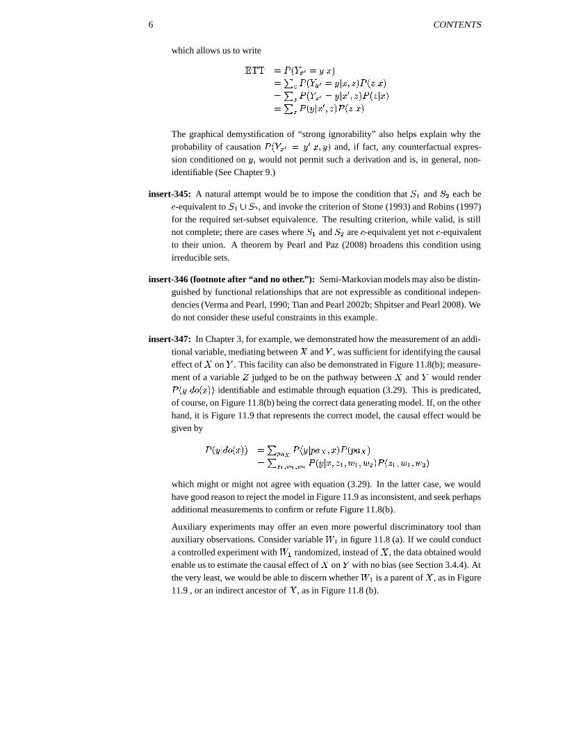
6 CONTENTS

which allows us to write

�� ' � � � ",% ' 9 ��' � � � �� "&% ' 9 � �� ' � � � �� "&% ' 9 �0�� ' � � � ��9 � ��

The graphical demystification of “strong ignorability” also helps explain why theprobability of causation � � � " % ' 9 � � �9 � and, if fact, any counterfactual expres-sion conditioned on 9 , would not permit such a derivation and is, in general, non-identifiable (See Chapter 9.)

insert-345: A natural attempt would be to impose the condition that � : and � < each be� -equivalent to � : � � < , and invoke the criterion of Stone (1993) and Robins (1997)for the required set-subset equivalence. The resulting criterion, while valid, is stillnot complete; there are cases where ��: and � < are � -equivalent yet not � -equivalentto their union. A theorem by Pearl and Paz (2008) broadens this condition usingirreducible sets.

insert-346 (footnote after “and no other.”): Semi-Markovian models may also be distin-guished by functional relationships that are not expressible as conditional indepen-dencies (Verma and Pearl, 1990; Tian and Pearl 2002b; Shpitser and Pearl 2008). Wedo not consider these useful constraints in this example.

insert-347: In Chapter 3, for example, we demonstrated how the measurement of an addi-tional variable, mediating between � and � , was sufficient for identifying the causaleffect of � on � . This facility can also be demonstrated in Figure 11.8(b); measure-ment of a variable � judged to be on the pathway between � and � would render� ��9 �� identifiable and estimable through equation (3.29). This is predicated,of course, on Figure 11.8(b) being the correct data generating model. If, on the otherhand, it is Figure 11.9 that represents the correct model, the causal effect would begiven by

� ��9 �� ' � *,+ 1 � ��9 � � � �� ' �� $ � $ � � � 9 �� : �� : �� < � � � � : �� : �� < �which might or might not agree with equation (3.29). In the latter case, we wouldhave good reason to reject the model in Figure 11.9 as inconsistent, and seek perhapsadditional measurements to confirm or refute Figure 11.8(b).

Auxiliary experiments may offer an even more powerful discriminatory tool thanauxiliary observations. Consider variable

� : in figure 11.8 (a). If we could conducta controlled experiment with

� : randomized, instead of � , the data obtained wouldenable us to estimate the causal effect of � on � with no bias (see Section 3.4.4). Atthe very least, we would be able to discern whether

� : is a parent of � , as in Figure11.9 , or an indirect ancestor of � , as in Figure 11.8 (b).

CONTENTS 7

In an attempt to adhere to traditional statistical methodology, some causal analystshave adopted an method called “sensitivity analysis” (e.g., Rosenbaum 2002, pp.105-170), which gives the impression that causal assumptions are not invoked in theanalysis. This, of course, is an illusion. Instead of drawing inferences by assumingthe absence of certain causal relationship in the model, the analyst tries such as-sumptions and evaluates how strong alternative causal relationships must be in orderto explain the observed data. The result is then submitted to a judgment of plausibil-ity, the nature it is no different from the judgments invoked in positing a model likethe one in Figure 11.9. In its richer setting, sensitivity analysis amounts to loadinga diagram with causal relationships whose strengths is limited by plausibility judg-ments and, given the data, attempting to draw conclusions without violating thoseplausibility constraints. It is a noble endeavor, which thus far has been limited toproblems with very small number of variables. The advent of diagrams promises toexpand the applicability of this method to more realistic problems.

insert-359: The method you are proposing, to replace the current equation � '�� with � ' �� , requires that we know the functional forms of � and� , as in linear systems or, alternatively, that the parents of � are observed, as inthe Process Control example on page 74. These do not hold, however, in the non-parametric, partially observable settings of Chapters 3 and 4, which might render itimpossible to predict the effect of the proposed intervention from data gathered priorto the intervention, a problem we called identification. Because pre-interventionstatistics is not available for variable � , and � is unknown, there are semi-Markoviancases where � ��9 �� is identifiable while � ��9 �� ' �� is not;each case must be analyzed on its own merit. It is important therefore to imposecertain standards on this vast space of potential interventions, and focus attention onthose that could illuminate others.

insert-360 (replace section 11.4.5):

11.4.5 Causation Without Manipulation!!!

Question to Author,In the analysis of direct effects, Section 4.5 invokes an example of sex discriminationin school admission and, in several of the formulas, gender is placed under the “hat”symbol or, equivalently, as an argument of the �� -operator. How can gender beplaced after the �� -operator when it is a variable that cannot be manipulated?

Author’s ReplySince Holland coined the unfortunate phrase “No Causation Without Manipulation”(Holland 1986) many good ideas were stifled or dismissed from causal analysis. Tosuppress talk about how gender causes the many biological, social and psychologicaldistinctions between males and females is to suppress 90% of our knowledge aboutgender differences.

8 CONTENTS

Surely we have causation without manipulation. The moon causes tides, race causesdiscrimination, and sex causes the secretion of certain hormones and not others. Na-ture is a society of mechanisms that relentlessly sense the values of some variablesand determine the values of others, and does not wait for a human manipulator beforeactivating those mechanisms.

True, manipulation is one way (albeit a crude one) for scientists to test the workingsof mechanisms, but it should not in any way inhibit causal thoughts, formal defini-tions and mathematical analyses of the mechanisms that propel the phenomena underinvestigation. It is for that reason, perhaps, that scientists invented counterfactuals;it permit them to state and conceive the realization of antecedent conditions withoutspecifying the physical means by which these conditions are established;

The purpose of the “hat” symbol in Definition 4.5.1 is not to stimulate thoughts aboutpossible ways of changing applicants’ gender, but to remind us that any definitionconcerned with “effects” should focus on causal links and filter out spurious associ-ations from the quantities defined. True, in the case of gender, one can safely replace� ��9 �� female � � with � � 9 female � , because the mechanism determining gender cansafely be assumed independent of the background factors that influence � (thus en-suring no confounding). But as a general definition, and even as part of an instructiveexample, mathematical expressions concerned with direct effects and sex discrimi-nation should maintain the hat symbol. If nothing else, placing “female” under the“hat” symbol should help propagate the long-overdue counter-slogan: “Causationwithout manipulation? You bet!”

insert-374: ... logic] of counterfactuals, is not given an explicit formal exposition: it isrelegated to a semi-formal [footnote...

insert-379: For completeness, I reiterate here explicitly (using parenthetical notation) thetwo fundamental connections between counterfactuals and structural equations.

1. The structural definition of counterfactuals is:

�� (' �� M �� Read: For any model and background information � , the counterfactualconditional “ � if � had been � ,” is given by the solution for � in submodel "

, (i.e., the mutilated version of with the equation determining � replacedby � ' � .)

2. The empirical claim of the structural equation 9�' � �� is:

� �� (' � �� for any set � not intersecting � or � .

Read: had � and � been � and � , respectively, � would be � �� , inde-pendently of � , and independently of other equations in the model.

CONTENTS 9

insert-394 (new paragraph): It is important to mention at this point that the canonicalpartition conception, coupled with the linear programming method developed inBalke and Pearl (1994a, 1995ab) has turned into a powerful analytical tool in avariety of applications. Tian and Pearl (2000) applied it to bound probabilities ofcausation; Kaufman et al. (2005) and Cai et al. (2008) used it to bound direct effectsin the presence of confounded mediation and, similarly, Imai et al. (2008) used it tobound natural direct and indirect effects. The closed-form expressions derived bythis method enable researchers to assess what features of the distribution are criticalfor narrowing the widths of the bounds.

Rubin (2004), in an independent exploration, attempted to apply canonical partitionsto the analysis of direct and indirect effects within the traditional potential-outcomeframework but, lacking the graphical and structural perspectives, was led to concludethat such effects are “ill-defined” and “more deceptive than helpful.” I believe readersof this book, guided by the structural roots of potential-outcome analysis, will reachmore positive conclusions (See Sections 4.5 and 11.4.2).

CONTENTS 1

ANSWERS TO RUSSELL’S QUESTIONSSECOND EDITION OF CAUSALITY (Updated 1/20/09)insert-251 should be :

satisfy the backdoor condition, because the inequality in Definition 7.5.1 can alwaysbe satisfied by conditioning on some imagined factor � (as in Figure 6.2 (c)) thatgenerates spurious associations between � and � .

insert 347 replace :the nature it is no different from the judgments invoked inwiththe nature of which is no different from the judgments invoked in

insert-159 (replace last sentence, 1st paragraph with) :Remarkably, graphical methods perform this computation without knowledge of � < ,� � and � �� < �� (Section 3.3.2).

This is indeed the essence of identifiability in nonparametric models. The ability toanswer interventional queries uniquely, from the data and the graph, is precisely howDefinition 3.2.3 interprets the identification of the causal effect � ��9 �� . As wehave seen in Chapters 3 and 4, that ability can be discerned graphically, almost byinspection, from the diagrams that accompany the equations.

page 443, replace :Pearl and Paz 2009 towith:Pearl and Paz 2008

page 444, replace :Pearl 2009 towith:Pearl 2008Also, Pearl 2008 should read “The mathematics of causal relations”

CONTENTS 1

“HOLD-OFF” CORRECTIONSNOT IMPLEMENTED

Updated 11/6/00

page 21 insert “Jensen, Cowles, Haddi, Neapolitan” - add to index?

page 141 per jp - do not add (9/11/2k) insert in 2nd paragraph, “Edwards 1995” before“Whittaker 1990”

page 269 insert in paragraph starting “The analysis of ACE...”. Insert “Heckman 1986;”before “Angrist and Imbens”

page 357 insert either “Summary” heading (before “I now wish” paragraph) or “***”(three stars centered)

page 361 add to citations: Edwards, D. (1995). Introduction to Graphical Modelling,New York: Springer-Verlag.

page 364 per jp, “keep for 2nd edition” 9/11/2k add to citations: Heckman, J.J., and R.R.Robb. (1986). Alternative Methods for Solving the Problem of Selection Bias inEvaluating the Impact of Treatments on Outcomes. In H. Wainer (Ed.), Drawing

Inferences from Self-Selected Samples, pp. 63–113. New York, NY: Springer-Verlag,

page 376 insert “Edwards, D., 141” before “Eells”

page 377 insert “Morgenstern, M., 183” before “Mueller”insert “Poole, C., 183” before “Poole, D.”

page 384 center tables, e.g. r. 299

CORRECTIONS/ADDITIONS TO NAME INDEXIN THE SECOND EDITION OF CAUSALITY

2/25/09 Updated

ADD TO AUTHOR INDEX

* designates new entry

Ader, H.: 172 (not 171)

Aldrich, J.: change 171 to 172

Angrist, J.D.: change 243-5 to 244-5

* Arah, O.A., 200

* Avin, C., 132

2 CONTENTS

Balke, A.: insert 70 and 257

Bayes, T.: insert 242

Bentler, P.: change 171 to 172

* Berk, _., 333 (double check insert/page number)

* Bessler, D., 64

Bollen, K.A.: remove 165, insert 172

Bonet, B.: insert 275, 308

* Brito, C., 171

* Brumback, B., 106

* Cai, Z., 126

Cartwright, N.: insert 106 and 172

* Chalak, K., 106

* Ciecro, _., 259 ????

* Cole, S.R., 129

Cowell, R.G.: insert 141

Cox, D.R.: insert 200, 340, 353

* Danks, D., 64, 253

Dawid, A.P.: insert 104-5, 111, 132, 141, check 341 epilogue

DeFenetti, B. (not De Fenetti)

* Demiralp, S., 64

Descartes, R., 335, 350 - check epilogue page #s

* Edwards, D., 141

* Elisseeff, A., 64

Fikes, R.E.: remove 725, insert 225

Fisher, R.A.: insert 127, check epilogue pages #s 340, 348, 353

* Frangakis, C.E., 264

(Fratiannea, A., 60) - remove

Freedman, D.A.: change 105 to 104-5

Galieo, G.: check epilogue page #s 334-6, 342

Galles, D.: remove 86 and 131, insert 257

Gallon, F.: check epilogue page # 339

Geiger, D.: change 12 to 11-2

* Geneletti, S., 132

* Gibbs, _., 270, 275-7, 280-1

Glymour, C.: change 63 to 63-4, insert 80, 106, 253

Goldberger, A.S.: change 171 to 172

Good, I.J.: insert 62

* Gopnik, A., 64, 253

Granger, C.W.J.: insert 64

Greenland, S.: remove 165 and 257, insert 106, 131, 271

Haavelmo, T.: insert 171

Hagenaars, J.: change 171 to 172

Hall, N.: change/insert 329 to 329-30

CONTENTS 3

Halpern, J.Y.: change/insert 329 to 329-30

* Hayduk, L., 172

Heckerman, D.: insert 211

Heckman, J.J.: insert 106, 139, 171-2, 216

* Herna’n, M.A., 106, 129

* Herna’ndez-Di’az, S. , 106

* Hiddleston, E., 330

Hitchcock, C.R., insert 330

Holland, P.W.: insert 106, remove 257

(Hollander, M., 281) - remove

(Holyoak, K.J., 60) - remove

Hoover, K.: insert 64, change 171 to 172

* Hopkins, M., 329

* Hoyer, P.O., 64

* Huang, Y., 86, 105

Hume, D.: check epilogue page #s 336, 343

Hurwicz, L.: insert 171

* Hyvarinen, A., 64

Imbens, G.W.: remove 243, (stet 244-5), insert 274-5

* Kano, Y., 64

* Kaufman, S., 106

* Kaufman, J.S., 106

* Kerminen, A.J., 64

Geng, p. 345 (add etal names)

Glymour, p. 64

Gopnik, p. 64 (add etal names)

Granger, p. 64

Greenland, p. 105 (add etal names), 130ish, 194ish, 345 (etal)

Haavelmo, p. 171

Hall, p. 330ish

Halpern, p. 329, 330ish

Heckman, p. 105, 171, 269

Hendry, p. 333

Hernan, p. 105 (add etal names), 129

Hiddleston, p. 330ish

Hitchcock, p. 330ish

4 CONTENTS

Holland, p. 105

Hoover, p. 64

Hopkins, p. 330ish

Howard, p. 111

Hoyer, p. 64 (add etal names)

Huang, p. 86, 105

Hurwicz, p. 171

Imbens, p. 269

Kaufmann, p. 105 (add etal names)

Kraus, p. 330ish (add etal names)

Lauritzen, p. 105

Maddala, p. 333

Marshak, p. 171

Matheson, p. 111?

McCabe, p. 200

Moneta, p. 64

Moore, p. 200

Morgan, p. 105, 171

Pearl, p. 11, 40, 41, 43, 64, 86, 105, 114, 130ish, 131ish, 171, 215ish, 269, 27

5, 329, 330ish, 344

Petersen, p. 105 (add etal names), 130ish (add etal names)

Rebane, p. 41, 43

Reichenbach, p. 43

Robb, p. 269

Robins, p. 64 (add etal names), 105, 130ish, 131ish, 344

Rosenbaum, p. 342, 349

Rothman, p. 194ish

Roy, p. 171

Rubin, p. 105, 264, 352

Rucker, p. 200

Salmon, p. 264

Scheines, p. 64

Schumacher, p. 200

Shimizu , p. 64 (add etal names)

Shpitser, p. 86, 105, 114, 131ish, 215ish

Spirtes, p. 64 (add etal names)

Spohn, p. 330ish

Stone, p. 344

Swanson, p. 64

Tian, p. 64, 105, 114, 345 (etal)

Valtorta, p. 86, 105?

VanderWeele, p. 105

Vytlacil, p. 171

CONTENTS 1

Wang, p. 345 (add etal names)

Wermuth, p. 40, 200

White, p. 105

Winship, p. 105, 171

Woodward, p. 105

MISSED CORRECTIONS/ADDITIONSIN THE SECOND EDITION OF CAUSALITY

2/25/09 Updated

Chapter 3

page 67, calligraphed � s begin to appear in chapter, not italicized as should be

page 72, footnote 4, line 3replace“said formula”with“this formula”

page 75, Notes:

� lowercase � s appear calligraphed, not italicized.� 1st and 2nd line in (3.16), subs under � are too small� in (3.17), sub under � is too small

page 86, paragraph after Corollary 3.4.2replaceWhether Rules 1–3 are sufficient for deriving all identifiable causal effects remainsan open question. However, the task of finding a sequence of transformations (if suchexists) for reducing an arbitrary causal effect expression can be systematized and ex-ecuted by efficient algorithms (Galles and Pearl 1995; Pearl and Robins 1995), tobe discussed in Chapter 4. As we illustrate in Section 3.4.3, symbolic derivationsusing the hat notation are much more convenient than algebraic derivations that aimat eliminating latent variables from standard probability expressions (as in Section3.3.2, equation (3.24)).withRules 1–3 have been shown to be complete, namely, sufficient for deriving all identi-fiable causal effects (Shpitser and Pearl 2006a; Huang and Valtorta 2006). Moreover,as illustrated in Section 3.4.3, symbolic derivations using the hat notation are moreconvenient than algebraic derivations that aim at eliminating latent variables fromstandard probability expressions (as in Section 3.3.2, equation(3.24)). However, thetask of deciding whether a sequence of rules exists for reducing an arbitrary causal

2 CONTENTS

effect expression has not been systematized, and direct graphical criteria for identifi-cation are therefore more desirable; see Theorem 3.6.1 and Chapter 4.

page 100, lines 1-2 after (3.53)replace“(an assumption that was termed “conditional ignorability” by Rosenbaum and Ru-bin 1983), then”with“(an assumption that was termed “conditional ignorability” by Rosenbaum and Ru-bin (1983)), then”

Chapter 4

page 108, paragraph 3, line 1replace“Traditional decision theory”with“Commonsensical decision theory”

page 109, 2nd paragraph, 2nd line of mnemonic rhymesreplaceOn facts that preceded the act,withOn what could have caused the act,

page 129, add sentence to end of footnote 8“Cole and Hernan (2002) present examples in epidemiology.”

page 132, in inserted page for 4.5.5, end of last sentence on pagereplace“Dawid (2000).”with“Dawid (2000) and Geneletti (2007).”

Chapter 8

page 264, replace“ Frangakis and Rubin (2002) dubbed them “Principal Stratification” and found themrather insightful. In the potential-outcome model (see Section 7.4.4),”with“In an experimental framework, this partition goes back to (Greenland and Robins1986) and was dubbed “Principlal Stratification” by Frangakis and Rubin (2002). Inthis framework (see Section 7.4.4),”

CONTENTS 3

Bibliography

page 447, correct in cites for Shimizu et al., 2005 and 2006should be “S. Shimizu” and “A. Hyvarinen” in both references

CONTENTS 1

CORRECTIONS TO THE SECOND EDITION OFCAUSALITY

4/15/09 Updated

throughout book: Replace “ACE*” with “ETT”

throughout book: No space between “Figure #” and (a) – i.e., Figure 11.8(a) (but not tooclose)

throughout book: Increase font size of subscripts, supscripts, subscript subs and sups,and supscript subs and sups

throughout book: Equalize the space between over/under bars and variables (i.e., � � )

throughout book: Equalize the space between hats and variables (i.e., �� )

throughout book: Font size of quoted materials fluctuates – keep larger as on page 238 ofthe 1st edition

throughout bibliography : Numbered editions are in numerical format, not written (i.e.,“2nd edition,” not “second edition”)

throughout bibliography : Numbered Proceedings are spelled out, not numerical (i.e.,“Seventh Proceedings,” not “7th Proceedings”)

page xix, Add new paragraph to the end of Preface of Second Edition (marked “insert-xix”)

I hope that each of these groups will find the unified approach taken in this book tobe both inspirational and instrumental in tackling new challenges in their respectivefields.

page 64 add new paragraph, “insert-64” as marked

Verma and Pearl (1990) noted that two latent structures may entail the same set ofconditional independencies and yet impose different equality constraints on the jointdistributions. These constraints, dubbed “dormant independencies,” were character-ized systematically in Tian and Pearl (2002b) and Shpitser and Pearl (2008); theypromise to provide a powerful new discovery tool for structure learning.

page 80, Replace: where the set � is called “sufficient set” (or “admissible”) for controlof confounding.With “insert-80”:where the set � is called “sufficient set;” admissible or deconfounding set is a betterterm.

2 CONTENTS

page 264, “insert-264”:In an experimental framework, this partition goes back to Greenland and Robins(1986) and was dubbed “Principlal Stratification” by Frangakis and Rubin (2002). Inthis framework

page 106, clarification of corrections, marked “insert-106”:

(2001), Hernan et al. (2002), Hernan et al. (2004), Greenland and Brumback (2002),Greenland et al. (1999ab), Kaufman et al. (2005), Petersen et al. (2006), Hernandez-Diaz et al. (2006), VanderWeele and Robins (2007), and Glymour and Greenland(2008).

Interesting applications of the front-door criterion (Section 3.3.2) were noted in so-cial science (Morgan and Winship 2007) and economics (Chalak and White 2006).

Some advocates of the “potential outcome” approach have been most resistant toaccepting graphs or structural equations as the basis for causal analysis and, lack-ing these conceptual tools, were unable to address the issue of covariate selection(Rosenbaum 2002, p. 76; Rubin 2007, 2008a) and were led to dismiss importantscientific concepts as “ill-defined,” “deceptive,” “confusing” (Holland 2001; Rubin2004, 2008b), and worse (Rubin 2009). Lauritzen (2004) and Heckman(2005) havecriticized this attitude.

page 131, replace last paragraph on page with

In particular, expression (4.12) is both valid and identifiable in Markovian models,where all �� -operators can be eliminated using Corollary 3.2.6; for example

� � � �� 4' )�� ' � �� ' � � � � = ��

page 385, paragraph 3, replace marked sentence with “insert-385”:

Your earlier statement describes the habitual, uncritical use of conditiong amongBayesian researchers, which occasionally lures the unwary into blind alleys (e.g.,Rubin (2009)):

Bibliography New entries:

Darwiche, 2009 A. Darwiche. Modeling and Reasoning with Bayesian Networks.Cambridge University Press, New York, 2009.

McDonald, 2002a R.P. McDonald. What can we learn from the path equations?:Identifiability, constraints, equivalence. Psychometrika, 67(2):225-249, 2002.

Pearl, 2009 J. Pearl. Letter to the Editor: Remarks on the method of propensityscores. Statistics in Medicine, 28:1415-1416, 2009.

CONTENTS 3

Rubin, 2009 D.B. Rubin. Author’s Reply: Should observational studies be designedto allow lack of balance in covariate distributions across treatment groups? Statistics

in Medicine, 28:1420-1423, 2009.

Shadish and Clark, 2006 W.R. Shadish and M.H. Clark. A radomized experimentcomparing random to nonrandom assignment. Unpublished Paper. University ofCalifornia. Merced, 2006.

Shrier, 2009 I. Shrier. Letter to the Editor: Propensity scores. Statistics in Medicine,28:1317-1318, 2009.

Sjolander, 2009 A. Sjolander. Letter to the Editor: Propensity scores and M-structures. Statistics in Medicine, 28:1416-1423, 2009.

4 CONTENTS

Name Index - additions/corrections:

Abbring, J.H., 399

Ader, H., 172

Aldrich, J., 28, 63, 97, 165, 172, 174, 183, 199

Alifiers, C., 64

Angrist, J.D., 90, 102, 170, 244-5, 247-8, 261, 269, 379

Arah, O.A., 200

Austin, P.C., 350

Avin, C., 132, 399

Balke, A., 37, 70, 90, 96, 202, 205, 213, 217, 257, 264, 267-71, 275, 281, 305, 389, 395

Bayes, T., 14, 73, 96, 224, 242

Battistin, E., 399

Bentler, P., 144, 152, 172

Berk, R.A., 333, 350-1

Bernoulli, J., 388

Bessler, D., 64, 398

Blalock, H.M., 138, 366

Bodkin, R.G., 136, 379

Bollen, K.A., 135, 141, 144, 148, 152, 159, 164, 172

Bonet, B., 236, 275, 308, 399

Bousmans, M., 399

Brito, C., 171, 366, 399

Brumback, B., 106

Butler, S.F., 399

Byerly, H.C., 399

Cai, Z., 126, 395, 398-9

Campbell, D.T., 351

CONTENTS 5

Cartwright, N., 41, 43, 60, 62, 106, 127-8, 136, 160-1, 172, 175, 221-2, 249, 254-7, 297,310, 314, 362-5, 374

Chakraborty, R., 399

Chalak, K., 106

Chen, H., 346

Cicero, 259

Clark, M.H., 350-1

Cole, S.R., 129

Cook, E.F., 196, 388

Cook, T.D., 351, 388

Cowell, R.G., 21, 141

Cox, D.R., 14, 22, 25, 76, 78, 81, 93, 97, 119, 141, 185, 200, 340, 353, 388

Danks, D., 64, 253

Darwiche, A., 21, 207

Dawid, A.P., 11, 18, 21, 34, 78, 104-5, 111, 132, 141, 206, 220, 264, 281, 297, 302, 374,382, 395-6, 399, 411

Decock, L., 399

DeFinetti, B., 178-9, 196, 386 [no space in name]

Dehejia, R.H., 350

de Leeuw, J., 350

Demiralp, S., 64

Descartes, R., 405, 420

Didelez, V., 399

Duncan, O.D., 351, 366

Edwards, D., 141

Elisseeff, A., 64

Fienberg, S.E., 72, 177, 396

Fikes, R.E., 114, 225

Fisher, R.A., 43, 127, 332, 410, 418, 423

6 CONTENTS

Frangakis, C.E., 264, 395

[remove, Fratiannea, A., 60]

Freedman, D.A., 41, 63, 97-8, 104-5, 134, 148, 164, 373, 397

Fung, W.K., 346

Galieo, G., 334-6, 412

Galles, D., 114, 116-7, 202, 204, 222, 230-1, 235-7, 243, 248, 257, 295

Gallon, F., 409

Geiger, D., 11-2, 18, 41, 60, 104, 142, 234

Geneletti, S., 132

Geng, Z., 199, 346

Gibbs, J.W., 21, 270, 275-7, 280-1

Gillies, D., 399

Glymour, C.N., 16, 18, 30, 41, 48, 50, 52, 60, 63-4, 70, 72, 79-80, 83, 86, 106, 108-9,142, 148, 150, 175, 179, 200, 204, 253, 300, 308, 329, 341 [added middle initial]

Goldberger, A.S., 28, 69, 97, 104, 134, 136, 148, 172, 215, 244

Good, I.J., 42, 55, 62, 74, 177, 222, 249, 254, 283-4, 297, 308, 310, 328-9

Gopnik, A., 64, 253

Granger, C.W.J., 39, 56, 64

Greenlander, S., 7, 80, 106, 131, 175, 183, 185, 187, 190, 193-200, 264, 271, 284-5, 290,292, 301, 308, 314, 341, 346, 353, 358, 388, 399

Guo, J., 346

Gursoy, K., 399

Haavelmo, T., 26, 68, 134-5, 137, 158, 171, 204, 365, 374, 377, 379-80

Hadlock, C.R., 399

Hagenaars, J., 172, 357, 399

Hall, N., 202, 313, 316, 325, 329-30

Halpern, J.Y., 202-3, 221, 231, 257, 318, 320, 329-30, 399

Hautaniemi, S., 399

Hayduk, L.A., 172, 366-7, 399

CONTENTS 7

Heckerman, D., 21, 41, 60, 64, 211, 264-5, 305

Heckman, J.J., 98, 106, 139, 165, 171-2, 229, 243, 248, 260, 269, 281, 350, 353, 364,374-9

Heise, D.R., 367

Hernan, M.A., 106, 129, 353

Hernandez-Diaz, S., 106, 353

Hiddleston, E., 330

Hitchcock, C.R., 108-9, 310, 330, 399

Holford, T.R., 196, 341

Holland, P.W., 35, 43, 54, 98, 102, 106, 134, 137-8, 162, 175, 177, 229, 244-5, 263, 334,361, 373

[remove, Hollander, M., 281]

[remove, Holyoak, K.J., 60]

Hoover, K.D., 64, 72, 160, 172, 314, 365, 374, 379, 399

Hopkins, M., 329, 399

Howard, R.A., 19, 76, 111, 382

Hoyer, P.O., 64, 399

Hsiao, C., 136, 379

Hsu, W., 399

Huang, Y., 86, 105

Hume, D., 41, 228, 238, 249, 406, 413

Hurwicz, L., 160, 171

Hyvarinen, A., 64

Ichimura, H., 350

Imai, K., 395

Imbens, G.W., 90, 102, 170, 244-5, 247-8, 261, 265, 269, 274-5, 281, 379

Intriligator, M.D., 136, 379

Judge, G.G., 379

Kang, C., 387

8 CONTENTS

Kano, Y., 64

Kaufman, J.S., 106, 353, 395

Kaufman, S., 106, 353, 395

Keele, L., 395

Kerminen, A.J., 64

Kenny, D., 398

Kraus, S., 330

Kuroki, M., 113, 126, 395, 398-9

Kushnir, T., 64, 253

Kyburg, H.E., 399

Laplace, P.S., 26, 96, 257

Lauritzen, S.L., 14, 16, 18-22, 104-6, 141, 281, 378

Lawry, J., 399

Leamer, E.E., 136, 165, 167, 172, 183 [correct name is “Leamer” not “Learner”]

Lehmann, D., 330

Lehmann, J., 398-9

Leroy, S.F., 136, 378, 399 [changed from LeRoy]

Lewis, D., 34-5, 37, 70, 112, 201-2, 225, 238-42, 309, 311, 313-5

Liebniz, G.W., 406

Lindley, D.V., 176-80, 196, 384, 399

Luellen, J.K., 350

MacLenose, R.F., 106, 353, 395

Maddala, G.S., 167-8, 334

Magidor, M., 330

Manski, C.F., 90, 98, 229, 243, 268, 281, 395

Markus, K.A., 398

Marschak, J., 70, 137, 158, 160, 171, 204, 374, 380

Matheson, J.E., 382

CONTENTS 9

McCabe, G.P., 200

McCarthy, J., 420

McDonald, R.P., 143, 163, 172, 366, 399

Megiddo, N., 380, 382, 386, 398

Miettinen, O.S., 196, 388

Miller, D.J., 379

Mitchell, A.A., 106

Miyakawa, M., 113, 126

Mittelhammer, R.C., 379

Moneta, A., 64

Moore, D.S., 200

Moreno, L., 350

Morgan, S.L., 106, 171, 243, 349-50, 353, 399

Morgenstern, H., 183, 194

Mulaik, S.A., 135, 159, 172, 399

Neuberg, L.G., 378, 399

Neyman, J., 66, 70, 96, 98, 102, 134, 180, 201, 205, 243, 333-4, 379

Novick, M.R., 176-80, 196

Occam, W., 42, 45-8

O’Rourke, J., 399

Orzol, S.M., 350

Payson, S., 399

Paz, A., 11-2, 80, 118, 234, 236-7, 346, 399

Pearl, J., 11-2, 14-22, 30-1, 37, 40-1, 43, 46-51, 55, 57, 59, 64, 68, 70, 72-3, 79-81, 85-6,90-1, 96, 101, 104-6, 109, 111, 113-4, 116-8, 121, 123, 125-6, 131-2, 142-3, 146,148, 150, 171-2, 175, 190, 198-200, 202, 204-5, 213, 215, 217, 221-2, 227, 230-2,234-7, 240, 243-4, 247-8, 252, 263-4, 268-9, 271, 275, 277, 294-6, 305, 316-8, 320,324, 329, 346, 351, 353, 355, 358, 363-4, 366, 373-4, 378, 382, 386-7, 389, 394-6,398

Pearson, K., 78, 105, 174, 176, 409-11, 424-5, 428

10 CONTENTS

Peikes, D.M. 350

Petersen, M.L., 106, 131, 353, 358

Pigeot, I., 399

Poole, C., 106, 183, 353

Rebane, G., 41, 43

Richard, J.F., 39, 97, 138, 162, 165, 167-9, 183, 245, 343

Richardson, T.S., 61, 141-2, 146-8, 150, 378 [added middle initial]

Rigdon, E.E., 399

Robb, R.R., 269

Robins, J.M., 35, 41, 72, 80, 90-1, 95, 99, 102-6, 118-21, 123, 125-6, 131, 175, 183, 187,189-90, 192, 196-200, 229, 244, 268, 271, 281, 284-5, 290, 292, 301, 341, 345-6,352-3, 358, 388

Rosen, D., 225

Rosenbaum, P.R., 70, 78, 80, 87, 92-3, 95, 100, 106, 229, 246, 289, 342, 348-52

Rothman, K.J., 183, 194-6, 283, 314, 353

Roy, A.D., 98, 171

Rubin, D.B., 35, 66, 70, 78, 80, 87, 90, 92, 95-6, 98, 100, 102, 134, 170, 175, 180, 185,201-2, 205, 243-8, 261, 264-5, 275, 289, 333-4, 342, 348-53, 379, 385, 395

Rucker, G.R., 200

Russell, B., 407-8, 413, 419

Savage, L.J., 386

Scheines, R., 16, 18, 30, 41, 48, 52, 60, 63-4, 70, 72, 79, 83, 86, 142, 148, 150, 175, 200,204

Schisterman, E.F., 106

Schumacker, M., 200

Schulz, L.E., 64, 253

Scott, S., 399

Shadish, W.R., 350-1

Shafer, G., 255, 255

CONTENTS 11

Shimizu, S., 64

Shipley, B., 142, 200, 359-60, 399

Shpitser, I., 64, 86, 105, 114, 118, 126, 132, 215, 346, 353-5, 390, 394-5, 399

Shrier, I., 351

Simon, H.A., 31, 68, 70, 137, 154, 158, 160, 172, 202, 204-5, 226-8, 257, 328-9, 378

Simpson, E.H., 78, 139, 173-82, 199-200, 424

Singpurwalla, N.D., 399

Sinisi, S.E., 106, 131, 353, 358

Sjolander, A., 351, 399

Skyrms, B., 43, 62, 74, 108, 208, 249, 385

Smith, D.E., 239-40

Smith, J., 350

Sobel, D.M., 64, 253

Speed, T.P., 14, 19, 30, 141, 411

Spiegelhalter, D.J., 20-1, 141

Spirtes, P., 16, 18, 30, 41, 48, 50, 52, 60-1, 63-4, 70, 72, 79, 83, 86, 96, 104, 142, 146-8,150, 175, 200, 204

Spohn, W., 11, 56, 249, 330

Stanley, J.D., 351

Stark, P.B., 397

Stigler, S., 200

Stone, R., 183, 187, 189-90, 199-200, 346

Strotz, R.H., 32, 70, 95-6, 204, 257, 374, 380

Suppes, P., 1-2, 42, 48, 55-6, 58, 62, 74, 235, 249, 255, 275, 407

Swanson, N.R., 64, 399

Tian, J., 64, 72, 80, 105, 114, 118, 147, 172, 294-6, 329, 346, 387, 395, 398-9

Todd, P., 350

Valtorta, M., 41, 86, 105

12 CONTENTS

van der Laan, M.J., 106, 131, 353, 358

VandeWeele, T.J., 106

Verma, T., 12, 18-9, 30, 46-7, 49-52, 64, 68, 104, 142-3, 146-8, 200, 234, 346

Vieta, F., 405

Vytlacil, E.J., 139, 171, 216, 248, 353, 374-8

[remove, Waldmann, M.R., 60]

Wang, X., 346

Wahba, S., 350

Wall, M., 399

Wasserman, L., 41, 64, 200

Weinberg, C.R., 78, 187, 196, 341, 353, 388

Werler, M.M., 106

Wermuth, N., 14, 22, 97-8, 104, 141, 148, 177, 199-200, 341, 353, 373

White, H., 106

Wickramaratne, P.J., 196, 341

Wilson, J., 368, 399

Winship, C., 106, 171, 243, 350, 353

Wold, H.O.A., 32, 70, 95-6, 204, 257, 374, 380, 417, 419

Woodward, J., 109, 160, 221, 239, 310, 329, 399

Wright, S., 26, 60, 67, 69, 134-5, 137-8, 140, 148, 360, 390, 415, 428

Xie, X., 346

Yamamoto, T., 395

Yudowsky, E.S., 353, 399

Yule, G.U., 176, 424

Zelterman, D., 399

Documents

CAUSALITY CORRECTIONS IMPLEMENTED IN 2nd PRINTING