Causality for Machine Learn- ing

39 Causality for Machine Learn-ingBernhard Schölkopf (Max Planck Institute for IntelligentSystems)

AbstractGraphical causal inference as pioneered by Judea Pearl arose from research on artificial intel-ligence (AI), and for a long time had little connection to the field of machine learning. Thischapter discusses where links have been and should be established, introducing key con-cepts along the way. It argues that the hard open problems of machine learning and AI areintrinsically related to causality, and explains how the field is beginning to understand them.

39.1 IntroductionThe machine learning community’s interest in causality has significantly increased in recentyears. My understanding of causality has been shaped by Judea Pearl and a number of col-laborators and colleagues, and much of it went into a book written with Dominik Janzing andJonas Peters [Peters et al. 2017]. I have spoken about this topic on various occasions,1 andsome of it is in the process of entering the machine learning mainstream, in particular theview that causal modeling can lead to more invariant or robust models. There is excitementabout developments at the interface of causality and machine learning, and the present arti-cle tries to put my thoughts into writing and draw a bigger picture. I hope it may not onlybe useful by discussing the importance of causal thinking for AI, but it can also serve as anintroduction to some relevant concepts of graphical or structural causal models (SCMs) for amachine learning audience.

In spite of all recent successes, if we compare what machine learning can do to what ani-mals accomplish, we observe that the former is rather bad at some crucial feats where animals

1 For example, Schölkopf [2017], talks at the International Conference on Learning Representations, the Asian Con-ference on Machine Learning, and in machine learning labs that have meanwhile developed an interest in causality(e.g., DeepMind); much of the present paper is essentially a written-out version of these talks.

1

2 Chapter 39 Causality for Machine Learning

excel. This includes transfer to new problems, and any form of generalization that is notfrom one data point to the next one (sampled from the same distribution), but rather fromone problem to the next one—both have been termed generalization, but the latter is a muchharder form thereof. This shortcoming is not too surprising since machine learning often disre-gards information that animals use heavily: interventions in the world, domain shifts, temporalstructure—by and large, we consider these factors a nuisance and try to engineer them away.Finally, machine learning is also bad at thinking in the sense of Konrad Lorenz, that is, actingin an imagined space.2 IQ1 will argue that causality, with its focus on modeling and reasoningabout interventions, can make a substantial contribution toward understanding and resolvingthese issues and thus take the field to the next level. I will do so mostly in non-technicallanguage, for many of the difficulties of this field are of a conceptual nature.

39.2 The Mechanization of Information ProcessingThe first industrial revolution began in the late 18th century and was triggered by the steamengine and waterpower. The second one started about a century later and was driven by elec-trification. If we think about it broadly, then both are about how to generate and convert formsof energy. Here, the word “generate” is used in a colloquial sense—in physics, energy is aconserved quantity and can thus not be created, but only converted or harvested from otherenergy forms. Some think we are now in the middle of another revolution, called the digitalrevolution, the big data revolution, and, more recently, the AI revolution. The transforma-tion, however, really started already in the mid-20th century under the name of cybernetics. Itreplaced energy by information. Like energy, information can be processed by people, but todo it at an industrial scale we needed to invent computers, and to do it intelligently we now useAI. Just like energy, information may actually be a conserved quantity, and we can probablyonly ever convert and process it, rather than generating it from thin air. When machine learningis applied in industry, we often convert user data into predictions about future user behaviorand thus money. Money may ultimately be a form of information—a view not inconsistentwith the idea of bitcoins generated by solving cryptographic problems. The first industrialrevolutions rendered energy a universal currency [Smil 2017]; the same may be happening toinformation.

Like for the energy revolution, one can argue that the present revolution has two compo-nents: the first one built on the advent of electronic computers, the development of high-levelprogramming languages, and the birth of the field of computer science, engendered by thevision to create AI by manipulation of symbols. The second one, which we are currentlyexperiencing, relies upon learning. It allows to extract information also from unstructureddata, and it automatically infers rules from data rather than relying on humans to conceive

2 “Ich sehe nicht, was Denken grundsätzlich anderes sein soll als ein solches probeweises und nur im Gehirn sichabspielendes Handeln im vorgestellten Raum” [Lorenz 1973].

39.2 The Mechanization of Information Processing 3

of and program these rules. While Judea’s approach arose out of classic AI, he was also oneof the first to recognize some of the limitations of hard rules programmed by humans, andthus led the way in marrying classic AI with probability theory [Pearl 1988]. This gave birthto graphical models, which were adopted by the machine learning community, yet largelywithout paying heed to their causal semantics. In recent years, genuine connections betweenmachine learning and causality have emerged, and we will argue that these connections arecrucial if we want to make progress on the major open problems of AI.

At the time, the invention of automatic means of processing energy transformed the world.It made human labor redundant in some fields, and it spawned new jobs and markets in others.The first industrial revolution created industries around coal, the second one around electricity.The first part of the information revolution built on this to create electronic computing and theIT industry, and the second part is transforming IT companies into “AI first” as well as creat-ing an industry around data collection and “clickwork.” While the latter provides labeled datafor the current workhorse of AI, supervised machine learning [Vapnik 1998], one may antici-pate that new markets and industries will emerge for causal forms of directed or interventionalinformation, as opposed to just statistical dependences.

The analogy between energy and information is compelling, but our present understandingof information is rather incomplete, as was the concept of energy during the course of thefirst two industrial revolutions. The profound modern understanding of the concept of energycame with the mathematician Emmy Noether, who understood that energy conservation isdue to a symmetry (or covariance) of the fundamental laws of physics: they look the sameno matter how we shift the time, in present, past, and future. Einstein, too, was relying oncovariance principles when he established the equivalence between energy and mass. Amongfundamental physicists, it is widely held that information should also be a conserved quantity,although this brings about certain conundrum especially in cosmology.3 One could speculatethat the conservation of information might also be a consequence of symmetries—this wouldbe most intriguing, and it would help us understand how different forms of (phenomenolog-ical) information relate to each other, and define a unified concept of information. We willbelow introduce a form of invariance/independence that may be able to play a role in thisrespect.4 The intriguing idea of starting from symmetry transformations and defining objectsby their behavior under these transformations has been fruitful not just in physics but also inmathematics [Klein 1872, MacLane 1971].3 What happens when information falls into a black hole? According to the no hair conjecture, a black hole seen fromthe outside is fully characterized by its mass, (angular) momentum, and charge.4 Mass seemingly played two fundamentally different roles (inertia and gravitation) until Einstein furnished a deeperconnection in general relativity. It is noteworthy that causality introduces a layer of complexity underlying thesymmetric notion of statistical mutual information. Discussing source coding and channel coding, Shannon [1959]remarked: “This duality can be pursued further and is related to a duality between past and future and the notions ofcontrol and knowledge. Thus we may have knowledge of the past but cannot control it; we may control the future buthave no knowledge of it.” According to Kierkegaard, “Life can only be understood backwards; but it must be livedforwards.”


Clearly, digital goods are different from physical goods in some respects, and the sameholds true for information and energy. A purely digital good can be copied at essentially zerocost [Brynjolfsson et al. 2019], unless we move into the quantum world [Wootters and Zurek1982]. The cost of copying a physical good, on the other hand, can be as high as the costof the original (e.g., for a piece of gold). In other cases, where the physical good has a non-trivial informational structure (e.g., a complex machine), copying it may be cheaper than theoriginal. In the first phase of the current information revolution, copying was possible forsoftware, and the industry invested significant effort in preventing this. In the second phase,copying extends to datasets, for given the right machine learning algorithm and computationalresources others can extract the same information from a dataset. Energy, in contrast, can onlybe used once.

Just like the first industrial revolutions had a major impact on technology, economy, andsociety, the same will likely apply for the current changes. It is arguably our information pro-cessing ability that is the basis of human dominance on this planet, and thus also of the majorimpact of humans on our planet. Since it is about information processing, the current revo-lution is thus potentially even more significant than the first two industrial revolutions. Weshould strive to use these technologies well to ensure they will contribute toward the solutionsof humankind’s and our planet’s problems. This extends from questions of ethical genera-tion of energy (e.g., environmental concerns) to ethical generation of information (privacy,clickwork) all the way to how we are governed. In the beginnings of the information revolu-tion, cybernetician Stafford Beer worked with Chile’s Allende government to build cyberneticgovernance mechanisms [Medina 2011]. In the current data-driven phase of this revolution,China is beginning to use machine learning to observe and incentivize citizens to behave inways deemed beneficial [Chen and Cheung 2018, Dai 2018]. It is hard to predict where thisdevelopment takes us—this is science fiction at best, and the best science fiction may provideinsightful thoughts on the topic.5

39.3 From Statistical to Causal Models39.3.1 Methods Driven by Independent and Identically Distributed Data

Our community has produced impressive successes with applications of machine learningto big data problems [LeCun et al. 2015]. In these successes there are multiple trends atwork: (1) we have massive amounts of data, often from simulations or large-scale humanlabeling, (2) we use high-capacity machine learning systems (i.e., complex function classeswith many adjustable parameters), (3) we employ high-performance computing systems, andfinally (often ignored, but crucial when it comes to causality) (4) the problems are independent

5 Quoting from Asimov [1951]: “Hari Seldon [..] brought the science of psychohistory to its full development. [..]The individual human being is unpredictable, but the reactions of humans mobs, Seldon found, could be treatedstatistically.”

39.3 From Statistical to Causal Models 5

and identically distributed (IID). The settings are typically either IID to begin with (e.g., imagerecognition using benchmark datasets), or they are artificially made IID, e.g., by carefullycollecting the right training set for a given application problem, or by methods such as Deep-Mind’s “experience replay” [Mnih et al. 2015] where a reinforcement learning agent storesobservations in order to later permute them for the purpose of further training. For IID data,strong universal consistency results from statistical learning theory apply, guaranteeing con-vergence of a learning algorithm to the lowest achievable risk. Such algorithms do exist, forinstance, nearest neighbor classifiers and support vector machines [Vapnik 1998, Schölkopfand Smola 2002, Steinwart and Christmann 2008]. Seen in this light, it is not surprising thatwe can indeed match or surpass human performance if given enough data. Machines oftenperform poorly, however, when faced with problems that violate the IID assumption yet seemtrivial to humans. Vision systems can be grossly misled if an object that is normally recog-nized with high accuracy is placed in a context that in the training set may be negativelycorrelated with the presence of the object. For instance, such a system may fail to recognizea cow standing on the beach. Even more dramatically, the phenomenon of “adversarial vul-nerability” highlights how even tiny but targeted violations of the IID assumption, generatedby adding suitably chosen noise to images (imperceptible to humans), can lead to danger-ous errors such as confusion of traffic signs. Recent years have seen a race between “defensemechanisms” and new attacks that appear shortly after and re-affirm the problem. Overall, itis fair to say that much of the current practice (of solving IID benchmark problems) as wellas most theoretical results (about generalization in IID settings) fail to tackle the hard openproblem of generalization across problems.

To further understand the way in which the IID assumption is problematic, let us consider ashopping example. Suppose Alice is looking for a laptop rucksack on the Internet (i.e., a ruck-sack with a padded compartment for a laptop), and the web store’s recommendation systemsuggests that she should buy a laptop to go along with the rucksack. This seems odd becauseshe probably already has a laptop, otherwise she would not be looking for the rucksack in thefirst place. In a way, the laptop is the cause and the rucksack is an effect. If I am told whethera customer has bought a laptop, it reduces my uncertainty about whether she also bought alaptop rucksack, and vice versa—and it does so by the same amount (the mutual information),so the directionality of cause and effect is lost. It is present, however, in the physical mech-anisms generating statistical dependence, for instance the mechanism that makes a customerwant to buy a rucksack once she owns a laptop. Recommending an item to buy constitutes anintervention in a system, taking us outside the IID setting. We no longer work with the obser-vational distribution, but a distribution where certain variables or mechanisms have changed.This is the realm of causality.

Reichenbach [1956] clearly articulated the connection between causality and statisticaldependence. He postulated the Common Cause Principle: if two observables X and Y are Q2sta-tistically dependent, then there exists a variable Z that causally influences both and explains


all the dependence in the sense of making them independent when conditioned on Z. As aspecial case, this variable can coincide with X or Y. Suppose that X is the frequency of storksand Y the human birth rate (in European countries, these have been reported to be correlated).If storks bring the babies, then the correct causal graph is X � Y . If babies attract storks, itis X � Y . If there is some other variable that causes both (such as economic development),we have X � Z � Y .

The crucial insight is that without additional assumptions, we cannot distinguish thesethree cases using observational data. The class of observational distributions over X and Y thatcan be realized by these models is the same in all three cases. A causal model thus containsgenuinely more information than a statistical one.

Given that already the case where we have two observables is hard, one might wonder ifthe case of more observables is completely hopeless. Surprisingly, this is not the case: theproblem in a certain sense becomes easier, and the reason for this is that in that case thereare non-trivial conditional independence properties [Spohn 1978, Dawid 1979, Geiger andPearl 1990] implied by causal structure. These can be described by using the language ofcausal graphs or SCMs, merging probabilistic graphical models and the notion of interven-tions [Spirtes et al. 2000, Pearl 2009a] best described using directed functional parent–childrelationships rather than conditionals. While conceptually simple in hindsight, this constituteda major step in the understanding of causality, as later expressed by Pearl (2009a, p. 104):

We played around with the possibility of replacing the parents–child relationshipP �Xi¶PAi� with its functional counterpart Xi � fi�PAi,Ui� and, suddenly, every-thing began to fall into place: We finally had a mathematical object to which wecould attribute familiar properties of physical mechanisms instead of those slipperyepistemic probabilities P �Xi¶PAi� with which we had been working so long in thestudy of Bayesian networks.

39.3.2 Structural Causal ModelsThe SCM viewpoint is intuitive for those machine learning researchers who are more accus-tomed to thinking in terms of estimating functions rather than probability distributions. In it,we are given a set of observables X1, . . . ,Xn (modelled as random variables) associated withthe vertices of a directed acyclic graph (DAG). We assume that each observable is the resultof an assignment

Xi �� fi�PAi,Ui�, �i � 1, . . . ,n�, (39.1)

using a deterministic function fi depending on Xi’s parents in the graph (denoted by PAi) andon a stochastic unexplained variable Ui. Directed edges in the graph represent direct cau-sation, since the parents are connected to Xi by directed edges and through Equation (39.1)directly affect the assignment of Xi. The noise Ui ensures that the overall object (39.1) can

39.3 From Statistical to Causal Models 7

represent a general conditional distribution p�Xi¶PAi�, and the set of noises U1, . . . ,Un areassumed to be jointly independent. If they were not, then by the Common Cause Principlethere should be another variable that causes their dependence, and thus our model would notbe causally sufficient.

If we specify the distributions of U1, . . . ,Un, recursive application of Equation (39.1)allows us to compute the entailed observational joint distribution p�X1, . . . ,Xn�. This dis-tribution has structural properties inherited from the graph [Lauritzen 1996, Pearl 2009a]:it satisfies the causal Markov condition stating that conditioned on its parents, each Xj isindependent of its non-descendants. Intuitively, we can think of the independent noises as“information probes” that spread through the graph (much like independent elements of gos-sip can spread through a social network). Their information gets entangled, manifesting itselfin a footprint of conditional dependences rendering the possibility to infer aspects of the graphstructure from observational data using independence testing. Like in the gossip analogy, thefootprint may not be sufficiently characteristic to pin down a unique causal structure. In par-ticular, it certainly is not if there are only two observables since any non-trivial conditionalindependence statement requires at least three variables.

We have studied the two-variable problem over the last decade. We realized that it can beaddressed by making additional assumptions, as not only the graph topology leaves a foot-print in the observational distribution but the functions fi do, too. This point is interestingfor machine learning, where much attention is devoted to properties of function classes (e.g.,priors or capacity measures), and we shall return to it below. Before doing so, we note twomore aspects of Equation (39.1). First, the SCM language makes it straightforward to formal-ize interventions as operations that modify a subset of assignments (39.1), e.g., changing Ui,or setting fi (and thus Xi) to a constant [Spirtes et al. 2000, Pearl 2009a]. Second, the graphstructure along with the joint independence of the noises implies a canonical factorization ofthe joint distribution entailed by Equation (39.1) into causal conditionals that we will refer toas the causal (or disentangled) factorization,

p�X1, . . . ,Xn� �n

5i�1

p�Xi¶PAi�. (39.2)

While many other entangled factorizations are possible, e.g.,

p�X1, . . . ,Xn� �n

5i�1

p�Xi¶Xi�1, . . . ,Xn�, (39.3)

Equation (39.2) is the only one that decomposes the joint distribution into conditionals cor-responding to the structural assignments (39.1). We think of these as the causal mechanismsthat are responsible for all statistical dependences among the observables. Accordingly, incontrast to Equation (39.3), the disentangled factorization represents the joint distribution asa product of causal mechanisms.


The conceptual basis of statistical learning is a joint distribution p�X1, . . . ,Xn� (whereoften one of the Xi is a response variable denoted as Y), and we make assumptions aboutfunction classes used to approximate, say, a regression E�Y ¶X�. Causal learning considersa richer class of assumptions and seeks to exploit the fact that the joint distribution possessesa causal factorization (Equation (39.2)). It involves the causal conditionals p�Xi¶PAi� [i.e.,the functions fi and the distribution of Ui in Equation (39.1)], how these conditionals relate toeach other, and interventions or changes that they admit. We shall return to this below.

39.4 Levels of Causal ModelingBeing trained in physics, I like to think of a set of coupled differential equations as the goldstandard in modelling physical phenomena. It allows us to predict the future behavior of asystem, to reason about the effect of interventions in the system, and—by suitable averagingprocedures—to predict statistical dependences that are generated by coupled time evolutions.6

It also allows us to gain insight in a system, explain its functioning, and in particular read offits causal structure: consider the coupled set of differential equations

dxdt� f�x�, x " Rd

, (39.4)

with initial value x�t0� � x0. The Picard–Lindelöf theorem states that at least locally, if f isLipschitz, there exists a unique solution x(t). This implies in particular that the immediatefuture of x is implied by its past values.

If we formally write this in terms of infinitesimal differentials dt and dx � x�t�dt��x�t�,we get:

x�t�dt� � x�t��dt �f�x�t��. (39.5)

From this, we can ascertain which entries of the vector x(t) determine the future of oth-ers x�t�dt�. This tells us that if we have a physical system whose physical mechanisms arecorrectly described using such an ordinary differential equation (39.4), solved for dx

dt(i.e., the

derivative only appears on the left-hand side), then its causal structure can be directly read off.While a differential equation is a rather complete description of a system, a statistical model

can be viewed as a much more superficial one. It usually does not talk about time; instead,it tells us how some of the variables allow prediction of others as long as experimental con-ditions do not change. For example, if we drive a differential equation system with certaintypes of noise, or we average over time, then it may be the case that statistical dependencesbetween components of x emerge, and those can then be exploited by machine learning. Sucha model does not allow us to predict the effect of interventions; however, its strength is that

6 Indeed, one could argue that all statistical dependences in the world are due to such coupling.

39.5 Independent Causal Mechanisms 9

Table 39.1 A simple taxonomy of models. The most detailed model (top) is a mechanistic or physicalone, usually in terms of differential equations. At the other end of the spectrum (bottom),we have a purely statistical model; this can be learned from data, but it often provides littleinsight beyond modeling associations between epiphenomena. Causal models can be seenas descriptions that lie in between, abstracting away from physical realism while retainingthe power to answer certain interventional or counterfactual questions. See also Mooij et al.[2013] for a formal link between physical models and SCMs.

Model Predict inIID setting

Predict underdistr. shift/intervention

Answercounter-factualquestions

Obtainphysicalinsight

Learnfromdata

Mechanistic/physical Yes Yes Yes Yes ?Structural causal Yes Yes Yes ? ?Causal graphical Yes Yes No ? ?Statistical Yes No No No Yes

it can often be learned from data, while a differential equation usually requires an intelligenthuman to come up with it. Causal modelling lies in between these two extremes. It aims toprovide understanding and predict the effect of interventions. Causal discovery and learningtries to arrive at such models in a data-driven way, using only weak assumptions.7 The overallsituation is summarized in Table 39.1, adapted from [Peters et al. 2017].

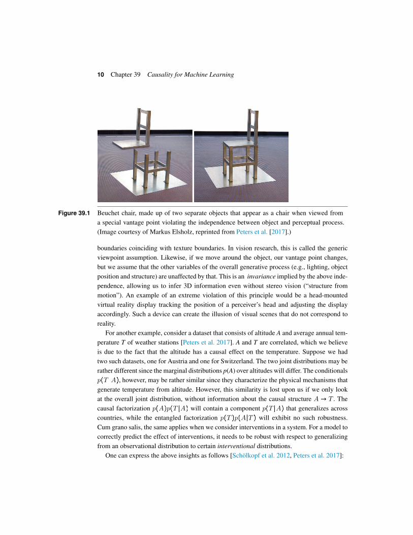
39.5 Independent Causal MechanismsWe now return to the disentangled factorization [Equation (39.2)] of the joint distributionp�X1, . . . ,Xn�. This factorization according to the causal graph is always possible when theUi are independent, but we will now consider an additional notion of independence relatingthe factors in Equation (39.2) to one another. We can informally introduce it using an opticalillusion known as the Beuchet chair, shown in Figure 39.1.

Whenever we perceive an object, our brain makes the assumption that the object and themechanism by which the information contained in its light reaches our brain are indepen-dent. We

Q3

can violate this by looking at the object from an accidental viewpoint. If we dothat, perception may go wrong: in the case of the Beuchet chair, we perceive the three-dimensional (3D) structure of a chair that in reality is not there. The above independenceassumption is useful because in practice it holds most of the time, and our brain thus relies onobjects being independent of our vantage point and the illumination. Likewise, there shouldnot be accidental coincidences, 3D structures lining up in two-dimensional (2D), or shadow

7 It has been pointed out that this task is impossible without assumptions, but this is similar for the (easier) problemsof machine learning from finite data. We always need assumptions when we perform non-trivial inference from data.


Figure 39.1 Beuchet chair, made up of two separate objects that appear as a chair when viewed froma special vantage point violating the independence between object and perceptual process.(Image courtesy of Markus Elsholz, reprinted from Peters et al. [2017].)

boundaries coinciding with texture boundaries. In vision research, this is called the genericviewpoint assumption. Likewise, if we move around the object, our vantage point changes,but we assume that the other variables of the overall generative process (e.g., lighting, objectposition and structure) are unaffected by that. This is an invariance implied by the above inde-pendence, allowing us to infer 3D information even without stereo vision (“structure frommotion”). An example of an extreme violation of this principle would be a head-mountedvirtual reality display tracking the position of a perceiver’s head and adjusting the displayaccordingly. Such a device can create the illusion of visual scenes that do not correspond toreality.

For another example, consider a dataset that consists of altitude A and average annual tem-perature T of weather stations [Peters et al. 2017]. A and T are correlated, which we believeis due to the fact that the altitude has a causal effect on the temperature. Suppose we hadtwo such datasets, one for Austria and one for Switzerland. The two joint distributions may berather different since the marginal distributions p(A) over altitudes will differ. The conditionalsp�T ¶A�, however, may be rather similar since they characterize the physical mechanisms thatgenerate temperature from altitude. However, this similarity is lost upon us if we only lookat the overall joint distribution, without information about the causal structure A� T . Thecausal factorization p�A�p�T ¶A� will contain a component p�T ¶A� that generalizes acrosscountries, while the entangled factorization p�T �p�A¶T � will exhibit no such robustness.Cum grano salis, the same applies when we consider interventions in a system. For a model tocorrectly predict the effect of interventions, it needs to be robust with respect to generalizingfrom an observational distribution to certain interventional distributions.

One can express the above insights as follows [Schölkopf et al. 2012, Peters et al. 2017]:


Independent Causal Mechanisms (ICM) Principle The causal generative process of a sys-tem’s variables is composed of autonomous modules that do not inform or influence eachother.In the probabilistic case, this means that the conditional distribution of each variable given

its causes (i.e., its mechanism) does not inform or influence the other mechanisms.

This principle subsumes several notions important to causality, including separate inter-venability of causal variables, modularity and autonomy of subsystems, and invariance [Pearl2009a, Peters et al. 2017]. If we have only two variables, it reduces to an independencebetween the cause distribution and the mechanism producing the effect distribution.

Applied to the causal factorization [Equation (39.2)], the principle tells us that the factorsshould be independent in the sense that

(a) changing (or intervening upon) one mechanism p�Xi¶PAi� does not change the othermechanisms p�Xj¶PAj� (i j j), and

(b) knowing some other mechanisms p�Xi¶PAi� (i j j) does not give us information abouta mechanism p�Xj¶PAj�.

Our notion of independence thus subsumes two aspects: the former pertaining to influenceand the latter to information.

We view any real-world distribution as a product of causal mechanisms. A change in sucha distribution (e.g., when moving from one setting/domain to a related one) will always be dueto changes in at least one of those mechanisms. Consistent with the independence principle,we hypothesize that smaller changes tend to manifest themselves in a sparse or local way, i.e.,they should usually not affect all factors simultaneously (sparse mechanism shift). In contrast,if we consider a non-causal factorization, for example, Equation (39.3), then many terms willbe affected simultaneously as we change one of the physical mechanisms responsible for asystem’s statistical dependences. Such a factorization may thus be called entangled, a termthat has gained popularity in machine learning [Bengio et al. 2012, Locatello et al. 2018a,Suter et al. 2018].

The notion of invariant, autonomous, and independent mechanisms has appeared in variousguises throughout the history of causality research.8 Our Q4contribution may be in unifying thesenotions with the idea of informational independence, and in showing that one can use rather

8 Early work on this was done by Haavelmo [1944], stating the assumption that changing one of the structural assign-ments leaves the other ones invariant. Hoover [2008] attributes to Herb Simon the invariance criterion: the true causalorder is the one that is invariant under the right sort of intervention. Aldrich [1989] provides an overview of the his-torical development of these ideas in economics. He argues that the “most basic question one can ask about a relationshould be: How autonomous is it?” [Frisch et al. 1948, Preface]. Pearl [2009a] discusses autonomy in detail, arguingthat a causal mechanism remains invariant when other mechanisms are subjected to external influences. He points outthat causal discovery methods may best work “in longitudinal studies conducted under slightly varying conditions,where accidental independencies are destroyed and only structural independencies are preserved.” Overviews areprovided by Aldrich [1989], Hoover [2008], Pearl [2009a], and Peters et al. [2017, section 2.2].


general independence measures [Steudel et al. 2010], a special case of which (algorithmicinformation) will be described below.Measures of dependence of mechanisms Note that the dependence of two mechanismsp�Xi¶PAi� and p�Xj¶PAj� does not coincide with the statistical dependence of the randomvariables Xi and Xj. Indeed, in a causal graph, many of the random variables will be dependenteven if all the mechanisms are independent.

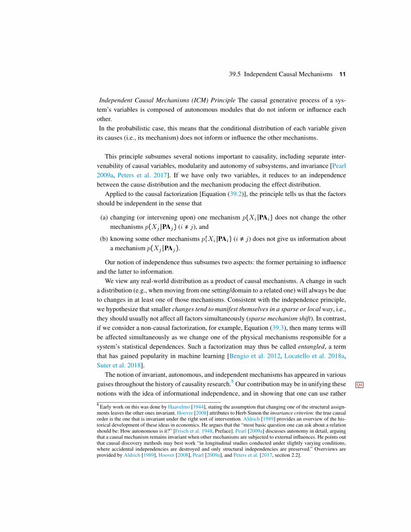
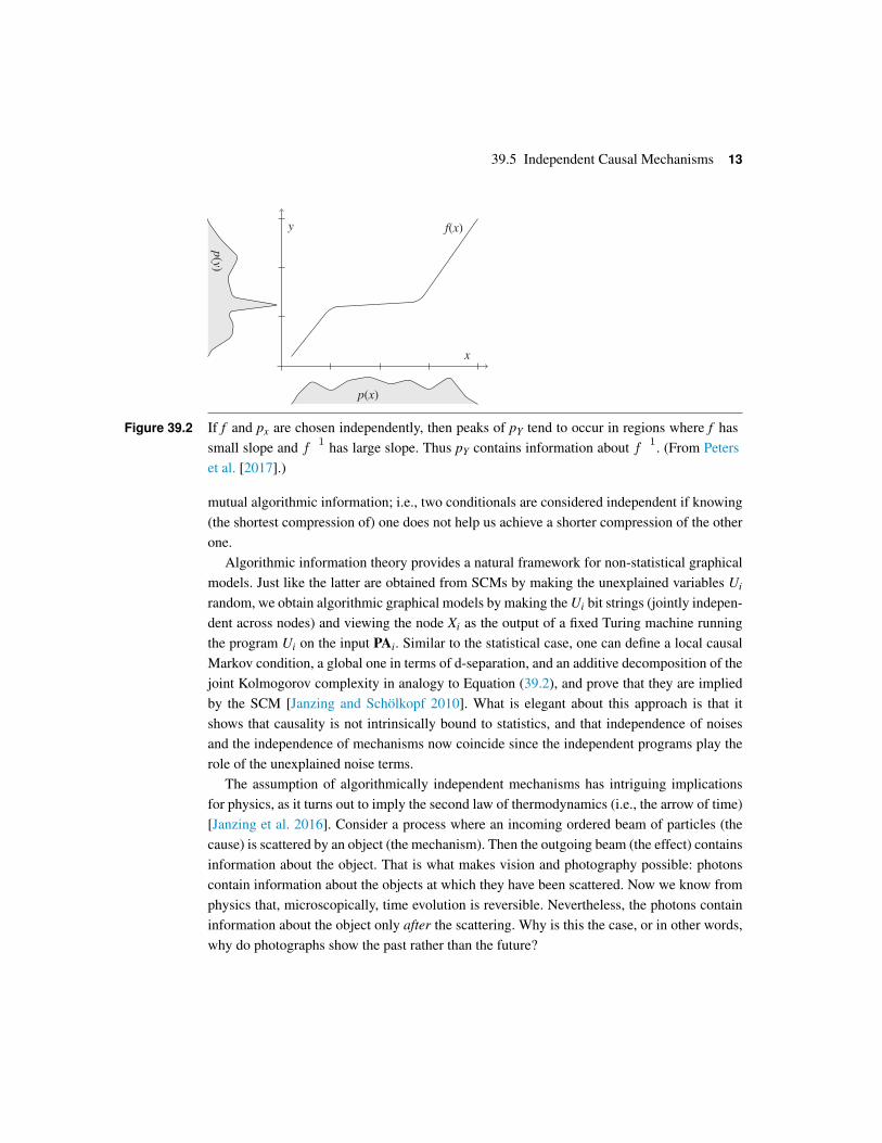
Intuitively speaking, the independent noise terms Ui provide and parametrize the uncer-tainty contained in the fact that a mechanism p�Xi¶PAi� is non-deterministic, and thus ensurethat each mechanism adds an independent element of uncertainty. I thus like to think of theICM Principle as containing the independence of the unexplained noise terms in an SCM[Equation (39.1)] as a special case.9 However, it goes beyond this, as the following exampleillustrates. Consider two variables and structural assignments X �� U and Y �� f�X�. Thatis, the cause X is a noise variable (with density pX), and the effect Y is a deterministic functionof the cause. Let us moreover assume that the ranges of X and Y are both [0, 1], and f is strictlymonotonically increasing. The principle of ICMs then reduces to the independence of pX and f.Let us consider pX and the derivative f ¬ as random variables on the probability space [0, 1] withLebesgue measure, and use their correlation as a measure of dependence of mechanisms.10

It can be shown that for f j id, independence of pX and f ¬ implies dependence between pY

and �f�1

�¬ (see Figure 39.2). Other measures are possible and admit information-geometric

interpretations. Intuitively, under the ICM assumption, the “irregularity” of the effect distri-bution becomes a sum of irregularity already present in the input distribution and irregularityintroduced by the function, i.e., the irregularities of the two mechanisms add up rather thancompensating each other, which would not be the case in the anticausal direction (for details,see Janzing et al. [2012]).Algorithmic independence So far, I have discussed links between causal and statistical struc-tures. The fundamental of the two is the causal structure, since it captures the physicalmechanisms that generate statistical dependences in the first place. The statistical structureis an epiphenomenon that follows if we make the unexplained variables random. It is awk-ward to talk about the (statistical) information contained in a mechanism since deterministicfunctions in the generic case neither generate nor destroy information. This motivated us todevise an algorithmic model of causal structures in terms of Kolmogorov complexity [Janz-ing and Schölkopf 2010]. The Kolmogorov complexity (or algorithmic information) of a bitstring is essentially the length of its shortest compression on a Turing machine, and thus ameasure of its information content. Independence of mechanisms can be defined as vanishing

9 See also Peters et al. [2017]. Note that one can also implement the independence principle by assigning indepen-dent priors for the causal mechanisms. We can view ICM as a meta-level independence, akin to assumptions oftime-invariance of the laws of physics [Bohm 1957].10 Other dependence measures have been proposed for high-dimensional linear settings and time series by Janzinget al. [2010], Shajarisales et al. [2015], Besserve et al. [2018a], and Janzing and Schölkopf [2018]; see also Janzing[2019].


y

x

f(x)

p(x)

p(y

)

Figure 39.2 If f and px are chosen independently, then peaks of pY tend to occur in regions where f hassmall slope and f

�1 has large slope. Thus pY contains information about f�1. (From Peters

et al. [2017].)

mutual algorithmic information; i.e., two conditionals are considered independent if knowing(the shortest compression of) one does not help us achieve a shorter compression of the otherone.

Algorithmic information theory provides a natural framework for non-statistical graphicalmodels. Just like the latter are obtained from SCMs by making the unexplained variables Ui

random, we obtain algorithmic graphical models by making the Ui bit strings (jointly indepen-dent across nodes) and viewing the node Xi as the output of a fixed Turing machine runningthe program Ui on the input PAi. Similar to the statistical case, one can define a local causalMarkov condition, a global one in terms of d-separation, and an additive decomposition of thejoint Kolmogorov complexity in analogy to Equation (39.2), and prove that they are impliedby the SCM [Janzing and Schölkopf 2010]. What is elegant about this approach is that itshows that causality is not intrinsically bound to statistics, and that independence of noisesand the independence of mechanisms now coincide since the independent programs play therole of the unexplained noise terms.

The assumption of algorithmically independent mechanisms has intriguing implicationsfor physics, as it turns out to imply the second law of thermodynamics (i.e., the arrow of time)[Janzing et al. 2016]. Consider a process where an incoming ordered beam of particles (thecause) is scattered by an object (the mechanism). Then the outgoing beam (the effect) containsinformation about the object. That is what makes vision and photography possible: photonscontain information about the objects at which they have been scattered. Now we know fromphysics that, microscopically, time evolution is reversible. Nevertheless, the photons containinformation about the object only after the scattering. Why is this the case, or in other words,why do photographs show the past rather than the future?


The reason is the independence principle, which we apply to initial state and systemdynamics, postulating that the two are algorithmically independent, that is, knowing one doesnot allow a shorter description of the other one. Then we can prove that the Kolmogorovcomplexity of the system’s state is non-decreasing under the time evolution. If we view Kol-mogorov complexity as a measure of entropy, this means that the entropy of the state can onlystay constant or increase, amounting to the second law of thermodynamics and providing uswith the thermodynamic arrow of time.

Note that this does not contradict microscopic irreversibility of the dynamics; the resultingstate after time evolution is clearly not independent of the system dynamic: it is precisely thestate that when fed to the inverse dynamics would return us to the original state, that is, theordered particle beam. If we were able to freeze all particles and reverse their momenta, wecould thus return to the original configuration without violating our version of the second law.

39.6 Cause–Effect DiscoveryLet us return to the problem of causal discovery from observational data. Subject to suitableassumptions such as faithfulness [Spirtes et al. 2000], one can sometimes recover aspects ofthe underlying graph from observations by performing conditional independence tests. How-ever, there are several problems with this approach. One is that in practice our datasets arealways finite, and conditional independence testing is a notoriously difficult problem, espe-cially if conditioning sets are continuous and multi-dimensional. So, while in principle theconditional independences implied by the causal Markov condition hold true irrespective ofthe complexity of the functions appearing in an SCM, for finite datasets conditional inde-pendence testing is hard without additional assumptions.11 The other problem is that in thecase of only two variables, the ternary concept of conditional independences collapses and theMarkov condition thus has no non-trivial implications.

It turns out that both problems can be addressed by making assumptions on functionclasses. This is typical for machine learning, where it is well-known that finite-sample general-ization without assumptions on function classes is impossible. Specifically, although there arelearning algorithms that are universally consistent, that is, that approach minimal expectederror in the infinite sample limit, for any functional dependence in the data there are caseswhere this convergence is arbitrarily slow. So, for a given sample size, it will depend on theproblem being learned whether we achieve low expected error, and statistical learning the-ory provides probabilistic guarantees in terms of measures of complexity of function classes[Devroye et al. 1996, Vapnik 1998].

Returning to causality, we provide an intuition why assumptions on the functions in anSCM should be necessary to learn about them from data. Consider a toy SCM with only two

11 We had studied this for some time with Kacper Chwialkowski, Arthur Gretton, Dominik Janzing, Jonas Peters, andIlya Tolstikhin; a formal result was obtained by Shah and Peters [2018].

39.6 Cause–Effect Discovery 15

observables X � Y . In this case, Equation (39.1) turns into

X � U (39.6)

Y � f�X,V � (39.7)

with U áá V. Now think of V acting as a random selector variable choosing from among a setof functions F � rfv�x� � f�x,v� ¶ v " supp�V �x. If f�x,v� depends on v in a non-smoothway, it should be hard to glean information about the SCM from a finite dataset, given thatV is not observed and it randomly switches between arbitrarily different fv.12 This motivatesrestricting the complexity with which f depends on V. A natural restriction is to assume anadditive noise model

X � U (39.8)

Y � f�X��V. (39.9)

If f in Equation (39.7) depends smoothly on V, and if V is relatively well concentrated, thiscan be motivated by a local Taylor expansion argument. It drastically reduces the effectivesize of the function class—without such assumptions the latter could depend exponentially onthe cardinality of the support of V.

Restrictions of function classes not only make it easier to learn functions from data, but itturns out that they can break the symmetry between cause and effect in the two-variable case:one can show that given a distribution over X,Y generated by an additive noise model, onecannot fit an additive noise model in the opposite direction (i.e., with the roles of X and Yinterchanged) [Hoyer et al. 2009, Mooij et al. 2009, Kpotufe et al. 2014, Peters et al. 2014,Bauer et al. 2016], cf. also the work of Sun et al. [2006]. This is subject to certain generic-ity assumptions, and notable exceptions include the case where U,V are Gaussian and f islinear. It generalizes the results of Shimizu et al. [2006] for linear functions, and it can begeneralized to include non-linear rescalings [Zhang and Hyvarinen 2009], loops [Mooij et al.2011], confounders [Janzing et al. 2009], and multi-variable settings [Peters et al. 2011]. Wehave collected a set of benchmark problems for cause–effect inference, and by now there isa number of methods that can detect causal direction better than chance [Mooij et al. 2016],some of them building on the above Kolmogorov complexity model [Budhathoki and Vreeken2016], and some directly learning to classify bivariate distributions into causal vs. anticausal

12 Suppose X and Y are binary, and U, V are uniform Bernoulli variables, the latter selecting from F � rid,notx (i.e.,identity and negation). In this case, the entailed distribution for Y is uniform, independent of X, even though we haveX � Y . We would be unable to discern X � Y from data.


[Lopez-Paz et al. 2015]. This development has been championed by Isabelle Guyon whom(along with Andre Elisseeff) I had known from my previous work on kernel methods, andwho had moved into causality through her interest in feature selection [Guyon et al. 2007].

Assumptions on function classes have thus helped address the cause–effect inference prob-lem. They can also help address the other weakness of causal discovery methods based onconditional independence testing. Recent progress in (conditional) independence testing heav-ily relies on kernel function classes to represent probability distributions in reproducing kernelHilbert spaces [Gretton et al. 2005a, 2005b, Fukumizu et al. 2008, Zhang et al. 2011, Chalupkaet al. 2018, Pfister et al. 2018b].

We have thus gathered some evidence that ideas from machine learning can help tacklecausality problems that were previously considered hard. Equally intriguing, however, is theopposite direction: can causality help us improve machine learning? Present-day machinelearning (and thus also much of modern AI) is based on statistical modelling, but as thesemethods becomes pervasive, their limitations are becoming apparent. I will return to this aftera short application interlude.

39.7 Half-sibling Regression and Exoplanet DetectionThe application described below builds on causal models inspired by additive noise modelsand the ICM assumption. By a stroke of luck, it enabled a recent breakthrough in astronomy,detailed at the end of the present section.

Launched in 2009, the National Aeronautics and Space Administration (NASA)’s Keplerspace telescope initially observed 150,000 stars over four years in search of exoplanet transits.These are events where a planet partially occludes its host star, causing a slight decrease inbrightness, often orders of magnitude smaller than the influence of instrument errors. Whenlooking at stellar light curves with our collaborators at New York University, we noticed thatnot only were these light curves very noisy, but the noise structure was often shared acrossstars that were light years apart. Since that made direct interaction of the stars impossible, itwas clear that the shared information was due to the instrument acting as a confounder. Wethus devised a method that (a) predicts a given star of interest from a large set of other starschosen such that their measurements contain no information about the star’s astrophysicalsignal, and (b) removes that prediction in order to cancel the instrument’s influence.13 Wereferred to the method as “half-sibling” regression since target and predictors share a parent,namely the instrument. The method recovers the random variable representing the desiredsignal almost surely (up to a constant offset), for an additive noise model, and subject to theassumption that the instrument’s effect on the star is in principle predictable from the otherstars [Schölkopf et al. 2016a].

13 For events that are localized in time (such as exoplanet transits), we further argued that the same applies for suitablychosen past and future values of the star itself, which can thus also be used as predictors.

39.8 Invariance, Robustness, and Semi-supervised Learning 17

Meanwhile, the Kepler spacecraft suffered a technical failure, which left it with only twofunctioning reaction wheels, insufficient for the precise spatial orientation required by theoriginal Kepler mission. NASA decided to use the remaining fuel to make further observa-tions, however the systematic error was significantly larger than before—a godsend for ourmethod designed to remove exactly these errors. We augmented it with models of exoplanettransits and an efficient way to search light curves, leading to the discovery of 36 planet can-didates [Foreman-Mackey et al. 2015], of which 21 were subsequently validated as bona fideexoplanets [Montet et al. 2015]. Four years later, astronomers found traces of water in theatmosphere of the exoplanet K2-18b—the first such discovery for an exoplanet in the habit-able zone, i.e., allowing for liquid water [Benneke et al. 2019, Tsiaras et al. 2019]. The planetturned out to be one that had been first been detected in our work [Foreman-Mackey et al.2015, exoplanet candidate EPIC 201912552].

39.8 Invariance, Robustness, and Semi-supervised LearningAround 2009 or 2010, we started getting intrigued by how to use causality for machine learn-ing. In particular, the “neural net tank urban legend”14 seemed to have something to say aboutthe matter. In this story, a neural net is trained to classify tanks with high accuracy, but subse-quently found to have succeeded by focusing on a feature (e.g., time of day or weather) thatcontained information about the type of tank only due to the data collection process. Sucha system would exhibit no robustness when tested on new tanks whose images were takenunder different circumstances. My hope was that a classifier incorporating causality could bemade invariant with respect to this kind of changes, a topic that I had earlier worked on usingnon-causal methods [Chapelle and Schölkopf 2002]. We started to think about connectionsbetween causality and covariate shift, with the intuition that causal mechanisms should beinvariant, and likewise any classifier building on learning these mechanisms. However, manymachine learning classifiers were not using causal features as inputs, and indeed, we noticedthat they more often seemed to solve anticausal problems, that is, they used effect features topredict a cause.

Our ideas relating to invariance matured during a number of discussions with Dominik,Jonas, Joris Mooij, Kun Zhang, Bob Williamson and others, from a departmental retreat inRingberg in April 2010 to a Dagstuhl workshop in July 2011. The pressure to bring them tosome conclusion was significantly stepped up when I received an invitation to deliver a Posnerlecture at the Neural Information Processing Systems conference. At the time, I was involvedin founding a new Max Planck Institute, and it was getting hard to carve out enough timeto make progress.15 Dominik and I thus decided to spend a week in a Black Forest holiday

14 For a recent account, cf. https://www.gwern.net/Tanks15 Meanwhile, Google was stepping up their activities in AI, and I even forwent the chance to have a personal meetingwith Larry Page to discuss this arranged by Sebastian Thrun.

https://www.gwern.net/Tanks


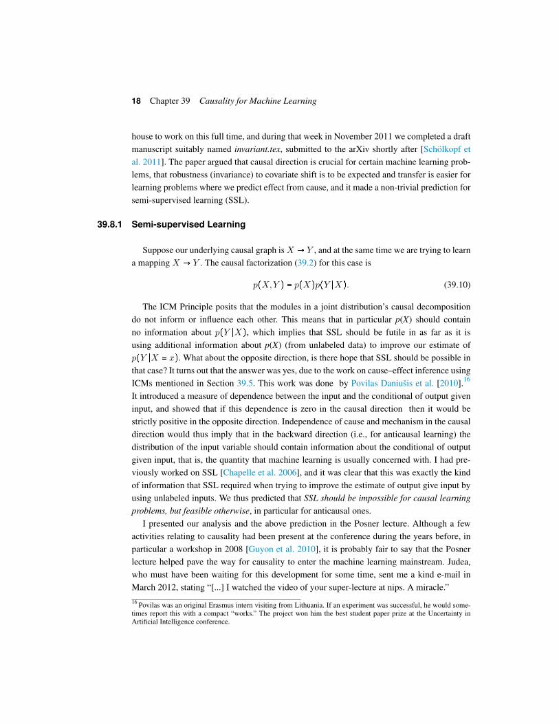
house to work on this full time, and during that week in November 2011 we completed a draftmanuscript suitably named invariant.tex, submitted to the arXiv shortly after [Schölkopf etal. 2011]. The paper argued that causal direction is crucial for certain machine learning prob-lems, that robustness (invariance) to covariate shift is to be expected and transfer is easier forlearning problems where we predict effect from cause, and it made a non-trivial prediction forsemi-supervised learning (SSL).

39.8.1 Semi-supervised Learning

Suppose our underlying causal graph is X� Y , and at the same time we are trying to learna mapping X � Y . The causal factorization (39.2) for this case is

p�X,Y � � p�X�p�Y ¶X�. (39.10)

The ICM Principle posits that the modules in a joint distribution’s causal decompositiondo not inform or influence each other. This means that in particular p(X) should containno information about p�Y ¶X�, which implies that SSL should be futile in as far as it isusing additional information about p(X) (from unlabeled data) to improve our estimate ofp�Y ¶X � x�. What about the opposite direction, is there hope that SSL should be possible inthat case? It turns out that the answer was yes, due to the work on cause–effect inference usingICMs mentioned in Section 39.5. This work was done by Povilas Daniušis et al. [2010].16

It introduced a measure of dependence between the input and the conditional of output giveninput, and showed that if this dependence is zero in the causal direction then it would bestrictly positive in the opposite direction. Independence of cause and mechanism in the causaldirection would thus imply that in the backward direction (i.e., for anticausal learning) thedistribution of the input variable should contain information about the conditional of outputgiven input, that is, the quantity that machine learning is usually concerned with. I had pre-viously worked on SSL [Chapelle et al. 2006], and it was clear that this was exactly the kindof information that SSL required when trying to improve the estimate of output give input byusing unlabeled inputs. We thus predicted that SSL should be impossible for causal learningproblems, but feasible otherwise, in particular for anticausal ones.

I presented our analysis and the above prediction in the Posner lecture. Although a fewactivities relating to causality had been present at the conference during the years before, inparticular a workshop in 2008 [Guyon et al. 2010], it is probably fair to say that the Posnerlecture helped pave the way for causality to enter the machine learning mainstream. Judea,who must have been waiting for this development for some time, sent me a kind e-mail inMarch 2012, stating “[...] I watched the video of your super-lecture at nips. A miracle.”16 Povilas was an original Erasmus intern visiting from Lithuania. If an experiment was successful, he would some-times report this with a compact “works.” The project won him the best student paper prize at the Uncertainty inArtificial Intelligence conference.


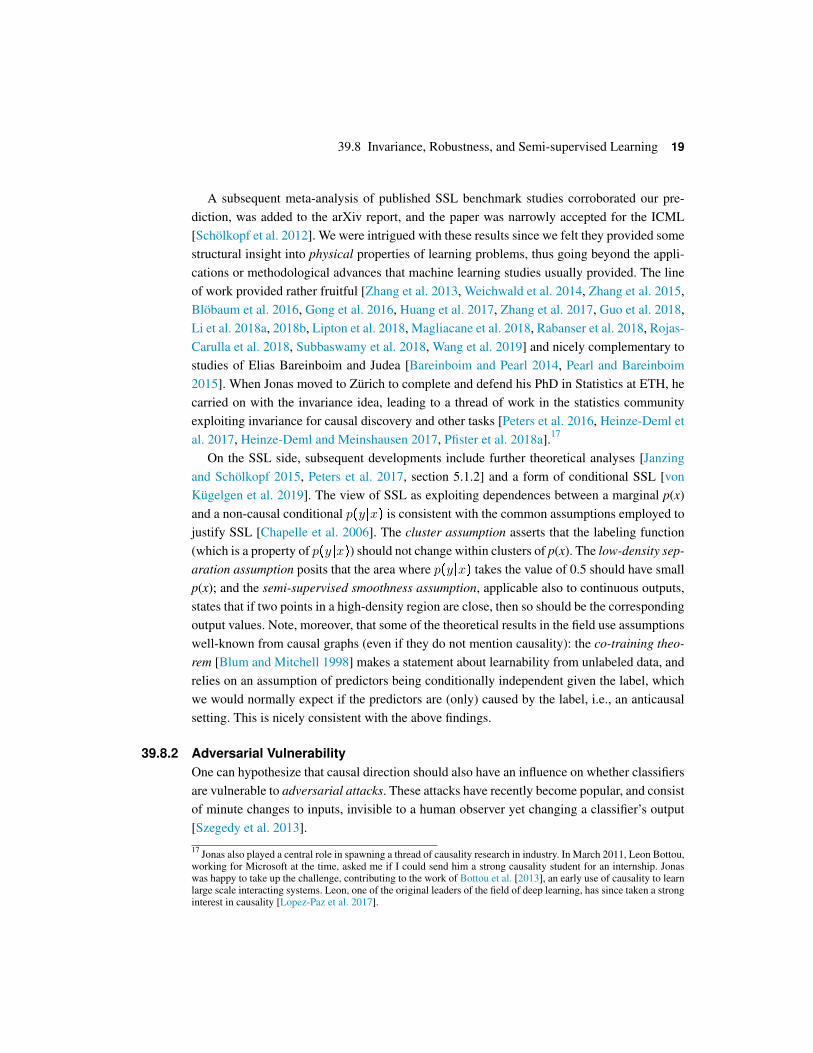
A subsequent meta-analysis of published SSL benchmark studies corroborated our pre-diction, was added to the arXiv report, and the paper was narrowly accepted for the ICML[Schölkopf et al. 2012]. We were intrigued with these results since we felt they provided somestructural insight into physical properties of learning problems, thus going beyond the appli-cations or methodological advances that machine learning studies usually provided. The lineof work provided rather fruitful [Zhang et al. 2013, Weichwald et al. 2014, Zhang et al. 2015,Blöbaum et al. 2016, Gong et al. 2016, Huang et al. 2017, Zhang et al. 2017, Guo et al. 2018,Li et al. 2018a, 2018b, Lipton et al. 2018, Magliacane et al. 2018, Rabanser et al. 2018, Rojas-Carulla et al. 2018, Subbaswamy et al. 2018, Wang et al. 2019] and nicely complementary tostudies of Elias Bareinboim and Judea [Bareinboim and Pearl 2014, Pearl and Bareinboim2015]. When Jonas moved to Zürich to complete and defend his PhD in Statistics at ETH, hecarried on with the invariance idea, leading to a thread of work in the statistics communityexploiting invariance for causal discovery and other tasks [Peters et al. 2016, Heinze-Deml etal. 2017, Heinze-Deml and Meinshausen 2017, Pfister et al. 2018a].17

On the SSL side, subsequent developments include further theoretical analyses [Janzingand Schölkopf 2015, Peters et al. 2017, section 5.1.2] and a form of conditional SSL [vonKügelgen et al. 2019]. The view of SSL as exploiting dependences between a marginal p(x)and a non-causal conditional p�y¶x� is consistent with the common assumptions employed tojustify SSL [Chapelle et al. 2006]. The cluster assumption asserts that the labeling function(which is a property of p�y¶x�) should not change within clusters of p(x). The low-density sep-aration assumption posits that the area where p�y¶x� takes the value of 0.5 should have smallp(x); and the semi-supervised smoothness assumption, applicable also to continuous outputs,states that if two points in a high-density region are close, then so should be the correspondingoutput values. Note, moreover, that some of the theoretical results in the field use assumptionswell-known from causal graphs (even if they do not mention causality): the co-training theo-rem [Blum and Mitchell 1998] makes a statement about learnability from unlabeled data, andrelies on an assumption of predictors being conditionally independent given the label, whichwe would normally expect if the predictors are (only) caused by the label, i.e., an anticausalsetting. This is nicely consistent with the above findings.

39.8.2 Adversarial VulnerabilityOne can hypothesize that causal direction should also have an influence on whether classifiersare vulnerable to adversarial attacks. These attacks have recently become popular, and consistof minute changes to inputs, invisible to a human observer yet changing a classifier’s output[Szegedy et al. 2013].

17 Jonas also played a central role in spawning a thread of causality research in industry. In March 2011, Leon Bottou,working for Microsoft at the time, asked me if I could send him a strong causality student for an internship. Jonaswas happy to take up the challenge, contributing to the work of Bottou et al. [2013], an early use of causality to learnlarge scale interacting systems. Leon, one of the original leaders of the field of deep learning, has since taken a stronginterest in causality [Lopez-Paz et al. 2017].


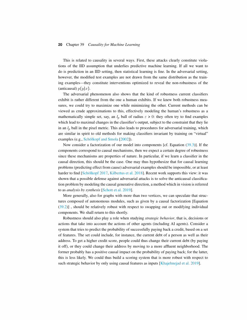
This is related to causality in several ways. First, these attacks clearly constitute viola-tions of the IID assumption that underlies predictive machine learning. If all we want todo is prediction in an IID setting, then statistical learning is fine. In the adversarial setting,however, the modified test examples are not drawn from the same distribution as the train-ing examples—they constitute interventions optimized to reveal the non-robustness of the(anticausal) p�y¶x�.

The adversarial phenomenon also shows that the kind of robustness current classifiersexhibit is rather different from the one a human exhibits. If we knew both robustness mea-sures, we could try to maximize one while minimizing the other. Current methods can beviewed as crude approximations to this, effectively modeling the human’s robustness as amathematically simple set, say, an lp ball of radius ε % 0: they often try to find exampleswhich lead to maximal changes in the classifier’s output, subject to the constraint that they liein an lp ball in the pixel metric. This also leads to procedures for adversarial training, whichare similar in spirit to old methods for making classifiers invariant by training on “virtual”examples (e.g., Schölkopf and Smola [2002]).

Now consider a factorization of our model into components [cf. Equation (39.3)]. If thecomponents correspond to causal mechanisms, then we expect a certain degree of robustnesssince these mechanisms are properties of nature. In particular, if we learn a classifier in thecausal direction, this should be the case. One may thus hypothesize that for causal learningproblems (predicting effect from cause) adversarial examples should be impossible, or at leastharder to find [Schölkopf 2017, Kilbertus et al. 2018]. Recent work supports this view: it wasshown that a possible defense against adversarial attacks is to solve the anticausal classifica-tion problem by modeling the causal generative direction, a method which in vision is referredto as analysis by synthesis [Schott et al. 2019].

More generally, also for graphs with more than two vertices, we can speculate that struc-tures composed of autonomous modules, such as given by a causal factorization [Equation(39.2)] , should be relatively robust with respect to swapping out or modifying individualcomponents. We shall return to this shortly.

Robustness should also play a role when studying strategic behavior, that is, decisions oractions that take into account the actions of other agents (including AI agents). Consider asystem that tries to predict the probability of successfully paying back a credit, based on a setof features. The set could include, for instance, the current debt of a person as well as theiraddress. To get a higher credit score, people could thus change their current debt (by payingit off), or they could change their address by moving to a more affluent neighborhood. Theformer probably has a positive causal impact on the probability of paying back; for the latter,this is less likely. We could thus build a scoring system that is more robust with respect tosuch strategic behavior by only using causal features as inputs [Khajehnejad et al. 2019].


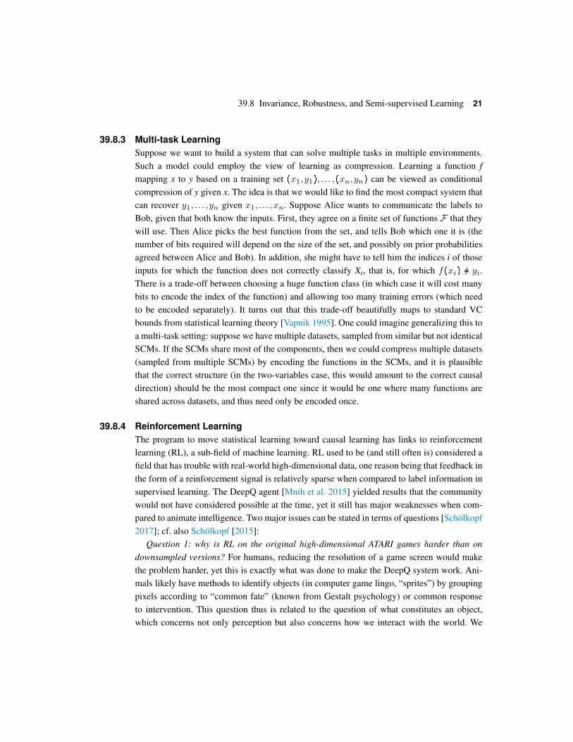
39.8.3 Multi-task LearningSuppose we want to build a system that can solve multiple tasks in multiple environments.Such a model could employ the view of learning as compression. Learning a function fmapping x to y based on a training set �x1,y1�, . . . ,�xn,yn� can be viewed as conditionalcompression of y given x. The idea is that we would like to find the most compact system thatcan recover y1, . . . ,yn given x1, . . . ,xn. Suppose Alice wants to communicate the labels toBob, given that both know the inputs. First, they agree on a finite set of functions F that theywill use. Then Alice picks the best function from the set, and tells Bob which one it is (thenumber of bits required will depend on the size of the set, and possibly on prior probabilitiesagreed between Alice and Bob). In addition, she might have to tell him the indices i of thoseinputs for which the function does not correctly classify Xi, that is, for which f�xi� j yi.There is a trade-off between choosing a huge function class (in which case it will cost manybits to encode the index of the function) and allowing too many training errors (which needto be encoded separately). It turns out that this trade-off beautifully maps to standard VCbounds from statistical learning theory [Vapnik 1995]. One could imagine generalizing this toa multi-task setting: suppose we have multiple datasets, sampled from similar but not identicalSCMs. If the SCMs share most of the components, then we could compress multiple datasets(sampled from multiple SCMs) by encoding the functions in the SCMs, and it is plausiblethat the correct structure (in the two-variables case, this would amount to the correct causaldirection) should be the most compact one since it would be one where many functions areshared across datasets, and thus need only be encoded once.

39.8.4 Reinforcement LearningThe program to move statistical learning toward causal learning has links to reinforcementlearning (RL), a sub-field of machine learning. RL used to be (and still often is) considered afield that has trouble with real-world high-dimensional data, one reason being that feedback inthe form of a reinforcement signal is relatively sparse when compared to label information insupervised learning. The DeepQ agent [Mnih et al. 2015] yielded results that the communitywould not have considered possible at the time, yet it still has major weaknesses when com-pared to animate intelligence. Two major issues can be stated in terms of questions [Schölkopf2017]; cf. also Schölkopf [2015]:

Question 1: why is RL on the original high-dimensional ATARI games harder than ondownsampled versions? For humans, reducing the resolution of a game screen would makethe problem harder, yet this is exactly what was done to make the DeepQ system work. Ani-mals likely have methods to identify objects (in computer game lingo, “sprites”) by groupingpixels according to “common fate” (known from Gestalt psychology) or common responseto intervention. This question thus is related to the question of what constitutes an object,which concerns not only perception but also concerns how we interact with the world. We


can pick up one object, but not half an object. Objects thus also correspond to modular struc-tures that can be separately intervened upon or manipulated. The idea that objects are definedby their behavior under transformation is a profound one not only in psychology but also inmathematics, cf. Klein [1872] and MacLane [1971].

Question 2: why is RL easier if we permute the replayed data? As an agent moves aboutin the world, it influences the kind of data it gets to see, and thus the statistics change overtime. This violates the IID assumption, and as mentioned earlier, the DeepQ agent stores andre-trains on past data (a process the authors liken to dreaming) in order to be able to employstandard IID function learning techniques. However, temporal order contains information thatanimate intelligence uses. Information is not only contained in temporal order but also in thefact that slow changes of the statistics effectively create a multi-domain setting. Multi-domaindata have been shown to help identify causal (and thus robust) features, and more generallyin the search for causal structure by looking for invariances [Peters et al. 2017]. This couldenable RL agents to find robust components in their models that are likely to generalize toother parts of the state space. One way to do this is to employ model-based RL using SCMs,an approach that can help address a problem of confounding in RL where time-varying andtime-invariant unobserved confounders influence both actions and rewards [Lu et al. 2018]. Insuch an approach, non-stationarities would be a feature rather than a bug, and agents wouldactively seek out regions that are different from the known ones in order to challenge theirexisting model and understand which components are robust. This search can be viewed andpotentially analyzed as a form of intrinsic motivation, a concept related to latent learning inEthology that has been gaining traction in RL [Chentanez et al. 2005].

Finally, a large open area in causal learning is the connection to dynamics. While we maynaively think that causality is always about time, most existing causal models do not (andneed not) talk about time. For instance, returning to our example of altitude and temperature,there is an underlying temporal physical process that ensures that higher places tend to becolder. On the level of microscopic equations of motion for the involved particles, there is aclear causal structure (as described above, a differential equation specifies exactly which pastvalues affect the current value of a variable). However, when we talk about the dependenceor causality between altitude and temperature, we need not worry about the details of thistemporal structure—we are given a dataset where time does not appear, and we can reasonabout how that dataset would look if we were to intervene on temperature or altitude. It isintriguing to think about how to build bridges between these different levels of description.Some progress has been made in deriving SCMs that describe the interventional behavior ofa coupled system that is in an equilibrium state and perturbed in an “adiabatic” way [Mooijet al. 2013], with generalizations to oscillatory systems [Rubenstein et al. 2018]. There is nofundamental reason why simple SCMs should be derivable in general. Rather, an SCM is ahigh-level abstraction of an underlying system of differential equations, and such an equation

39.9 Causal Representation Learning 23

can only be derived if suitable high-level variables can be defined [Rubenstein et al. 2017],which is probably the exception rather than the rule.

RL is closer to causality research than the machine learning mainstream in that it some-times effectively directly estimates do-probabilities. For example, on-policy learning esti-mates do-probabilities for the interventions specified by the policy (note that these may notbe hard interventions if the policy depends on other variables). However, as soon as off-policylearning is considered, in particular in the batch (or observational) setting [Lange et al. 2012],issues of causality become subtle [Gottesman et al. 2018, Lu et al. 2018]. Recent work devotedto the field between RL and causality includes Bareinboim et al. [2015], Bengio et al. [2017],Buesing et al. [2018], Lu et al. [2018], Dasgupta et al. [2019], and Zhang and Bareinboim[2019].

39.9 Causal Representation LearningTraditional causal discovery and reasoning assumes that the units are random variables con-nected by a causal graph. Real-world observations, however, are usually not structured intothose units to begin with, for example, objects in images [Lopez-Paz et al. 2017]. The emerg-ing field of causal representation learning hence strives to learn these variables from data,much like machine learning went beyond symbolic AI in not requiring that the symbols thatalgorithms manipulate be given a priori (cf. Bonet and Geffner [2019]). Defining objects orvariables that are related by causal models can amount to coarse-graining of more detailedmodels of the world. Subject to appropriate conditions, structural models can arise fromcoarse-graining of microscopic models, including microscopic structural equation models[Rubenstein et al. 2017], ordinary differential equations [Rubenstein et al. 2018], and tempo-rally aggregated time series [Gong et al. 2017]. Although every causal models in economics,medicine, or psychology uses variables that are abstractions of more elementary concepts, itis challenging to state general conditions under which coarse-grained variables admit causalmodels with well-defined interventions [Chalupka et al. 2015, Rubenstein et al. 2017].

The task of identifying suitable units that admit causal models is challenging for bothhuman and machine intelligence, but it aligns with the general goal of modern machinelearning to learn meaningful representations for data, where meaningful can mean robust,transferable, interpretable, explainable, or fair [Kusner et al. 2017, Kilbertus et al. 2017,Zhang and Bareinboim 2018]. To combine structural causal modeling [Equation (39.1)] andrepresentation learning, we should strive to embed an SCM into larger machine learning mod-els whose inputs and outputs may be high-dimensional and unstructured, but whose innerworkings are at least partly governed by an SCM. A way to do so is to realize the unexplainedvariables as (latent) noise variables in a generative model. Note, moreover, that there is a nat-ural connection between SCMs and the modern generative models: they both use what hasbeen called the reparametrization trick [Kingma and Welling 2013], consisting of making


desired randomness an (exogenous) input to the model (in an SCM, these are the unexplainedvariables) rather than an intrinsic component.

39.9.1 Learning Transferable MechanismsAn artificial or natural agent in a complex world is faced with limited resources. This con-cerns training data, that is, we only have limited data for each individual task/domain, andthus need to find ways of pooling/re-using data, in stark contrast to the current industry prac-tice of large-scale labeling work done by humans. It also concerns computational resources:animals have constraints on the size of their brains, and evolutionary neuroscience knowsmany examples where brain regions get re-purposed. Similar constraints on size and energyapply as ML methods get embedded in (small) physical devices that may be battery powered.Future AI models that robustly solve a range of problems in the real world will thus likelyneed to re-use components, which requires that the components are robust across tasks andenvironments [Schölkopf et al. 2016b]. An elegant way to do this is to employ a modularstructure that mirrors a corresponding modularity in the world. In other words, if the worldis indeed modular, in the sense that different components of the world play roles across arange of environments, tasks, and settings, then it would be prudent for a model to employcorresponding modules [Goyal et al. 2019]. For instance, if variations of natural lighting (theposition of the sun, clouds, etc.) imply that the visual environment can appear in brightnessconditions spanning several orders of magnitude, then visual processing algorithms in ournervous system should employ methods that can factor out these variations, rather than build-ing separate sets of face recognizers, say, for every lighting condition. If our brain were tocompensate for the lighting changes by a gain control mechanism, say, then this mechanismin itself need not have anything to do with the physical mechanisms bringing about bright-ness differences. It would, however, play a role in a modular structure that corresponds tothe role the physical mechanisms play in the world’s modular structure. This could producea bias toward models that exhibit certain forms of structural isomorphism to a world that wecannot directly recognize, which would be rather intriguing, given that ultimately our brainsdo nothing but turn neuronal signals into other neuronal signals.

A sensible inductive bias to learn such models is to look for ICMs [Locatello et al. 2018b],and competitive training can play a role in this: for a pattern recognition task, Parascandoloet al. [2018] show that learning causal models that contain independent mechanisms helps intransferring modules across substantially different domains. In this work, handwritten charac-ters are distorted by a set of unknown mechanisms including translations, noise, and contrastinversion. A neural network attempts to undo these transformations by means of a set of mod-ules that over time specialize on one mechanism each. For any input, each module attempts toproduce a corrected output, and a discriminator is used to tell which one performs best. Thewinning module gets trained by gradient descent to further improve its performance on thatinput. It is shown that the final system has learned mechanisms such as translation, inversion,

39.9 Causal Representation Learning 25

or denoising, and that these mechanisms transfer also to data from other distributions, such asSanskrit characters. This has recently been taken to the next step, embedding a set of dynamicmodules into a recurrent neural network, coordinated by a so-called attention mechanism[Goyal et al. 2019]. This allows learning modules whose dynamics operate independentlymuch of the time but occasionally interact with each other.

39.9.2 Learning Disentangled RepresentationsWe have earlier discussed the ICM Principle implying both the independence of the SCMnoise terms in Equation (39.1) and thus the feasibility of the disentangled representation

p�S1, . . . ,Sn� �n

5i�1

p�Si¶PAi� (39.11)

as well as the property that the conditionals p�Si¶PAi� be independently manipulable andlargely invariant across related problems. Suppose we seek to reconstruct such a disentangledrepresentation using independent mechanisms [Equation (39.11)] from data, but the causalvariables Si are not provided to us a priori. Rather, we are given (possibly high-dimensional)X � �X1, . . . ,Xd� (below, we think of X as an image with pixels X1, . . . ,Xd), from whichwe should construct causal variables S1, . . . ,Sn (n8d) as well as mechanisms, cf. Equation(39.1),

Si �� fi�PAi,Ui�,�i � 1, . . . ,n�, (39.12)

modeling the causal relationships among the Si. To this end, as a first step, we can use anencoder q � Rd

� Rn taking X to a latent “bottleneck” representation comprising the unex-plained noise variables U � �U1, . . . ,Un�. The next step is the mapping f (U) determined bythe structural assignments f1, . . . ,fn.18 Finally, we apply a decoder p � Rn

� Rd. If n is suf-ficiently large, the system can be trained using reconstruction error to satisfy p`f `q � id onthe observed images.19 To make it causal, we use the ICM Principle, that is, we should makethe Ui statistically independent, and we should make the mechanisms independent. This canbe done by ensuring that they be invariant across problems, or that they can be indepen-dently intervened upon: if we manipulate some of them, they should thus still produce validimages, which could be trained using the discriminator of a generative adversarial network[Goodfellow et al. 2014].18 Note that for a DAG, recursive substitution of structural assignments reduces them to functions of the noisevariables only. Using recurrent networks, cyclic systems may be dealt with.19 If the causal graph is known, the topology of a neural network implementing f can be fixed accordingly; if not,the neural network decoder learns the composition p � p` f . In practice, one may not know f, and thus only learnan autoencoder p` q, where the causal graph effectively becomes an unspecified part of p. By choosing the networktopology, one can ensure that each noise should only feed into one subsequent unit (using connections skippinglayers), and that all DAGs can be learnt.


While we ideally manipulate causal variables or mechanisms, we discuss the special caseof intervening upon the latent noise variables.20 One way to intervene is to replace noisevariables with the corresponding values computed from other input images, a procedure thathas been referred to as hybridization by Besserve et al. [2018b]. In the extreme case, wecan hybridize latent vectors where each component is computed from another training exam-ple. For an IID training set, these latent vectors have statistically independent components byconstruction.

In such an architecture, the encoder is an anticausal mapping that recognizes or reconstructscausal drivers in the world. These should be such that in terms of them mechanisms can beformulated that are transferable (e.g., across tasks). The decoder establishes the connectionbetween the low-dimensional latent representation (of the noises driving the causal model)and the high-dimensional world; this part constitutes a causal generative image model. TheICM assumption implies that if the latent representation reconstructs the (noises driving the)true causal variables, then interventions on those noises (and the mechanisms driven by them)are permissible and lead to valid generation of image data.

39.9.3 Learning Interventional World Models and ReasoningModern representation learning excels at learning representations of data that preserve rele-vant statistical properties [Bengio et al. 2012, LeCun et al. 2015]. It does so, however, withouttaking into account causal properties of the variables, that is, it does not care about the inter-ventional properties of the variables it analyzes or reconstructs. I expect that going forwardcausality will play a major role in taking representation learning to the next level, movingbeyond the representation of statistical dependence structures toward models that supportintervention, planning, and reasoning, realizing Konrad Lorenz’s notion of thinking as actingin an imagined space. This ultimately requires the ability to reflect back on one’s actions andenvision alternative scenarios, possibly necessitating (the illusion of) free will [Pearl 2009b].The biological function of self-consciousness may be related to the need for a variable rep-resenting oneself in one’s Lorenzian imagined space, and free will may then be a means tocommunicate about actions taken by that variable, crucial for social and cultural learning, atopic that has not yet entered the stage of machine learning research although it is at the coreof human intelligence [Henrich 2016].

39.10 Personal Notes and ConclusionMy first conscious encounter with Judea Pearl was in 2001, at a symposium on the Interfaceof Computing Sciences and Statistics.21 We both spoke at this symposium, and I recall histalk, formalizing an area of scientific inquiry that I had previously considered solidly part of

20 Interventions on the Si can be done accordingly, including the case of decoders without encoder (e.g., GANs).21 https://www.ics.uci.edu/~interfac/

https://www.ics.uci.edu/~interfac/

39.10 Personal Notes and Conclusion 27

the realm of philosophy. It stirred the same fascination that had attracted me to the researchthat I was doing at that time, in statistical learning theory and kernel methods. I had a back-ground in mathematics and physics, had dabbled in neural networks, and was impressed whenin 1994 I met Vladimir Vapnik, who taught me a statistical theory underlying the philosoph-ical problems of induction and generalization. Judea Pearl, another giant of our still youngfield of AI, seemed to be doing the same on a rather different but equally fascinating prob-lem. Like Vladimir, Judea left me with a lasting impression as someone who has mastered notjust technicalities but has gained access to profound philosophical understanding. With kernelmethods and learning theory taking off, I did not manage to go into depth on causality at thetime. I did follow some of the work in graphical models which became a staple in machinelearning, and I knew that although most researchers shied away from presenting these modelsas causal, this interpretation existed and formed a conceptual motivation for that field.

I was brought in touch with causality research for the second time in 2004 by my studyfriend Dominik Janzing. He was at the time working on quantum information, and spokeabout causality in a course he taught in Karlsruhe. The student Xiaohai Sun followed thatlecture and convinced Dominik to start working with him on a project. Eventually, the ques-tion of a PhD project came up, and Dominik (who felt his own field was too far from that)decided to ask me whether a joint supervision would make sense. At the time, Vladimir Vap-nik was visiting my lab, and after a long conversation, he agreed this could be interesting(“you should decide if you want to play this game”—by his standards, a fairly enthusiasticendorsement). I decided to take the risk, Xiaohai became a student in my lab in Tübingen, andin 2007, Dominik joined us. We also recruited the student Jonas Peters, who had taken partin a summer course I had taught in 2006, as well as the postdocs Joris Mooij and Kun Zhang,both independently driven toward the problem of causality. With Andre Elisseeff and SteffenLauritzen, Dominik and I wrote a proposal to organize a causality workshop in Dagstuhl. Thisworkshop took place in 2009, and helped us become members of the causality community; itwas where I first personally met Peter Spirtes.

I feel fortunate to have had such a strong team of people to do this work (including manywhom I did not mention by name above), and I believe we have made a contribution to moderncausality research and especially its links to machine learning: both by using learning meth-ods to develop data-driven causal methods, and by using inspiration from causality to betterunderstand machine learning and develop new learning methods. In that respect, representa-tion learning and disentanglement are intriguing fields. I recall a number of discussions withYoshua Bengio when I was a member of the review panel and advisory board of the CIFARprogram. He was driven by the goal to disentangle the underlying factors of variation in datausing deep learning, and I was arguing that this is a causal question. Our opinions have sincethen converged, and research has started to appear that combines both fields [Goudet et al.2017, Locatello et al. 2018a, Suter et al. 2018, Bengio et al. 2019, Goyal et al. 2019].


All this is still in its infancy, and the above account is personal and thus biased—I apolo-gize for any omissions. With the current hype around machine learning, there is much to sayin favor of some humility toward what machine learning can do, and thus toward the currentstate of AI—the hard problems have not been solved yet, making basic research in this fieldall the more exciting.

AcknowledgmentsMany thanks to all past and present members of the Tübingen causality team, without whosework and insights this article would not exist, in particular to Dominik Janzing and ChaochaoLu who read a version of the manuscript. The text has also benefitted from discussions withElias Bareinboim, Yoshua Bengio, Christoph Bohle, Leon Bottou, Anirudh Goyal, IsabelleGuyon, Judea Pearl, and Vladimir Vapnik. Wouter van Amsterdam, and Julius von Kügelgenhave pointed out typos that have been corrected in this second version.

References 29

ReferencesJ. Aldrich. 1989. Autonomy. Oxf. Econ. Pap. 41, 15–34. DOI: https://doi.org/10.1093/oxfordjournals.

oep.a041889.

I. Asimov. 1951. Foundation. Gnome Press, New York, NY.

E. Bareinboim and J. Pearl. 2014. Transportability from multiple environments with limited experi-ments: Completeness results. In Advances in Neural Information Processing Systems 27, 280–288.

E. Bareinboim, A. Forney, and J. Pearl. 2015. Bandits with unobserved confounders: A causalapproach. In Advances in Neural Information Processing Systems 28, 1342–1350.

S. Bauer, B. Schölkopf, and J. Peters. 2016. The arrow of time in multivariate time series. In Proceed-ings of the 33rd International Conference on Machine Learning, vol. 48 of JMLR Workshop andConference Proceedings, 2043–2051.

Y. Bengio, A. Courville, and P. Vincent. 2012. Representation learning: A review and new perspec-tives. IEEE Trans. Softw. Eng. 35, 8, 1798–1828. DOI: https://doi.org/10.1109/TPAMI.2013.50.

E. Bengio, V. Thomas, J. Pineau, D. Precup, and Y. Bengio. 2017. Independently controllable features.arXiv:1703.07718.

Y. Bengio, T. Deleu, N. Rahaman, R. Ke, S. Lachapelle, O. Bilaniuk, A. Goyal, and C. Pal. 2019. Ameta-transfer objective for learning to disentangle causal mechanisms. arXiv:1901.10912.

B. Benneke, I. Wong, C. Piaulet, H. A. Knutson, I. J. M. Crossfield, J. Lothringer, C. V. Morley, P.Gao, T. P. Greene, C. Dressing, D. Dragomir, A. W. Howard, P. R. McCullough, E. M. R. K. J. J.Fortney, and J. Fraine. 2019. Water vapor on the habitable-zone exoplanet K2-18b. arXiv:1909.04642.

M. Besserve, N. Shajarisales, B. Schölkopf, and D. Janzing. 2018a. Group invariance principles forcausal generative models. In Proceedings of the 21st International Conference on Artificial Intelli-gence and Statistics (AISTATS). 557–565.

M. Besserve, R. Sun, and B. Schölkopf. 2018b. Counterfactuals uncover the modular structure of deepgenerative models. arXiv:1812.03253.

P. Blöbaum, T. Washio, and S. Shimizu. 2016. Error asymmetry in causal and anticausal regression.Behaviormetrika 2017. arXiv:1610.03263. DOI: https://doi.org/10.1007/s41237-017-0022-z.

A. Blum and T. Mitchell. 1998. Combining labeled and unlabeled data with co-training. In Proceed-ings of the Eleventh Annual Conference on Computational Learning Theory. ACM, New York, NY,92–100. DOI: https://doi.org/10.1145/279943.279962.

D. Bohm. 1957. Causality and Chance in Modern Physics. Routledge & Kegan Paul, London.

B. Bonet and H. Geffner. 2019. Learning first-order symbolic representations for planning from thestructure of the state space. arXiv:1909.05546.

L. Bottou, J. Peters, J. Quiñonero-Candela, D. X. Charles, D. M. Chickering, E. Portugualy, D. Ray,P. Simard, and E. Snelson. 2013. Counterfactual reasoning and learning systems: The example ofcomputational advertising. J. Mach. Learn. Res. 14, 3207–3260.

https://doi.org/10.1093/oxfordjournals.oep.a041889

https://doi.org/10.1093/oxfordjournals.oep.a041889

https://doi.org/10.1109/TPAMI.2013.50

https://doi.org/10.1007/s41237-017-0022-z

https://doi.org/10.1145/279943.279962


E. Brynjolfsson, A. Collis, W. E. Diewert, F. Eggers, and K. J. Fox. 2019. GDP-B: Accounting for thevalue of new and free goods in the digital economy. Working Paper 25695, National Bureau of Eco-nomic Research.

K. Budhathoki and J. Vreeken. 2016. Causal inference by compression. In IEEE 16th InternationalConference on Data Mining. DOI: https://doi.org/10.1109/ICDM.2016.0015.

L. Buesing, T. Weber, Y. Zwols, S. Racaniere, A. Guez, J.-B. Lespiau, and N. Heess. 2018. Woulda,coulda, shoulda: Counterfactually-guided policy search. arXiv:1811.06272.

K. Chalupka, P. Perona, and F. Eberhardt. 2015. Multi-level cause–effect systems. arXiv:1512.07942.

K. Chalupka, P. Perona, and F. Eberhardt. 2018. Fast conditional independence test for vector variableswith large sample sizes. arXiv:1804.02747.

O. Chapelle and B. Schölkopf. 2002. Incorporating invariances in nonlinear SVMs. In T. G. Dietterich,S. Becker, and Z. Ghahramani (Eds.), Advances in Neural Information Processing Systems 14. MITPress, Cambridge, MA, 609–616.

O. Chapelle, B. Schölkopf, and A. Zien (Eds.). 2006. Semi-Supervised Learning. MIT Press, Cam-bridge, MA. http://www.kyb.tuebingen.mpg.de/ssl-book/. DOI: https://doi.org/10.7551/mitpress/9780262033589.001.0001.

Y. Chen and A. Cheung. 2018. The transparent self under big data profiling: Privacy and Chinese legis-lation on the social credit system. J. Comp. Law 12, 2, 356–378. DOI: http://dx.doi.org/10.2139/ssrn.2992537.

N. Chentanez, A. G. Barto, and S. P. Singh. 2005. Intrinsically motivated reinforcement learning. InAdvances in Neural Information Processing Systems 17. MIT Press, 1281–1288.

X. Dai. 2018. Toward a reputation state: The social credit system project of China. https://ssrn.com/abstract=3193577. DOI: http://dx.doi.org/10.2139/ssrn.3193577.

P. Daniušis, D. Janzing, J. M. Mooij, J. Zscheischler, B. Steudel, K. Zhang, and B. Schölkopf. 2010.Inferring deterministic causal relations. In Proceedings of the 26th Annual Conference on Uncer-tainty in Artificial Intelligence (UAI). 143–150.

I. Dasgupta, J. Wang, S. Chiappa, J. Mitrovic, P. Ortega, D. Raposo, E. Hughes, P. Battaglia, M.Botvinick, and Z. Kurth-Nelson. 2019. Causal reasoning from meta-reinforcement learning.arXiv:1901.08162.

A. P. Dawid. 1979. Conditional independence in statistical theory. J. R. Stat. Soc. B 41, 1, 1–31.

L. Devroye, L. Györfi, and G. Lugosi. 1996. A Probabilistic Theory of Pattern Recognition,Vol.31: Applications of Mathematics. Springer, New York, NY. DOI: http://dx.doi.org/10.1007/978-1-4612-0711-5.

D. Foreman-Mackey, B. T. Montet, D. W. Hogg, T. D. Morton, D. Wang, and B. Schölkopf. 2015. Asystematic search for transiting planets in the K2 data. Astrophys. J. 806, 2. http://stacks.iop.org/0004-637X/806/i=2/a=215. DOI: http://dx.doi.org/10.1088/0004-637X/806/2/215.

R. Frisch, T. Haavelmo, T. Koopmans, and J. Tinbergen. 1948. Autonomy of Economic Relations. Uni-versitets Socialøkonomiske Institutt, Oslo, Norway.

K. Fukumizu, A. Gretton, X. Sun, and B. Schölkopf. 2008. Kernel measures of conditional depen-dence. In Advances in Neural Information Processing Systems 20. 489–496.

https://doi.org/10.1109/ICDM.2016.0015

http://www.kyb.tuebingen.mpg.de/ssl-book/

https://doi.org/10.7551/mitpress/9780262033589.001.0001


http://dx.doi.org/10.2139/ssrn.2992537


https://ssrn.com/abstract=3193577

https://ssrn.com/abstract=3193577


http://dx.doi.org/10.1007/978-1-4612-0711-5

http://dx.doi.org/10.1007/978-1-4612-0711-5

http://stacks.iop.org/0004-637X/806/i=2/a=215

http://stacks.iop.org/0004-637X/806/i=2/a=215

http://dx.doi.org/10.1088/0004-637X/806/2/215

Chapter 39 Causality for Machine Learning 31

D. Geiger and J. Pearl. 1990. Logical and algorithmic properties of independence and their applica-tion to Bayesian networks. Ann. Math. Artif. Intell. 2, 165–178. DOI: https://doi.org/10.1007/BF01531004.

M. Gong, K. Zhang, T. Liu, D. Tao, C. Glymour, and B. Schölkopf. 2016. Domain adaptation withconditional transferable components. In Proceedings of the 33rd International Conference onMachine Learning. 2839–2848.

M. Gong, K. Zhang, B. Schölkopf, C. Glymour, and D. Tao. 2017. Causal discovery from temporallyaggregated time series. In Proceedings of the Thirty-Third Conference on Uncertainty in ArtificialIntelligence (UAI). ID 269.

I. Goodfellow, J. Pouget-Abadie, M. Mirza, B. Xu, D. Warde-Farley, S. Ozair, A. Courville, and Y.Bengio. 2014. Generative adversarial nets. In Advances in Neural Information Processing Systems27. Curran Associates, Inc., 2672–2680.

O. Gottesman, F. Johansson, J. Meier, J. Dent, D. Lee, S. Srinivasan, L. Zhang, Y. Ding, D. Wihl, X.Peng, J. Yao, I. Lage, C. Mosch, L. wei H. Lehman, M. Komorowski, M. Komorowski, A. Faisal,L. A. Celi, D. Sontag, and F. Doshi-Velez. 2018. Evaluating reinforcement learning algorithms inobservational health settings. arXiv:1805.12298.

O. Goudet, D. Kalainathan, P. Caillou, I. Guyon, D. Lopez-Paz, and M. Sebag. 2017. Causal generativeneural networks. arXiv:1711.08936.

A. Goyal, A. Lamb, J. Hoffmann, S. Sodhani, S. Levine, Y. Bengio, and B. Schölkopf. 2019. Recurrentindependent mechanisms. arXiv:1909.10893.

A. Gretton, O. Bousquet, A. Smola, and B. Schölkopf. 2005a. Measuring statistical dependence withHilbert–Schmidt norms. In Algorithmic Learning Theory. Springer-Verlag, 63–78. DOI: https://doi.org/10.1007/11564089_7.

A. Gretton, R. Herbrich, A. Smola, O. Bousquet, and B. Schölkopf. 2005b. Kernel methods for mea-suring independence. J. Mach. Learn. Res. 6, 2075–2129.

R. Guo, L. Cheng, J. Li, P. R. Hahn, and H. Liu. 2018. A survey of learning causality with data: Prob-lems and methods. arXiv:1809.09337. DOI: https://doi.org/10.1145/3397269.

I. Guyon, C. Aliferis, and A. Elisseeff. 2007. Causal feature selection. In Computational Methods ofFeature Selection. Chapman and Hall/CRC, 75–97.

I. Guyon, D. Janzing, and B. Schölkopf. 2010. Causality: Objectives and assessment. In I. Guyon, D.Janzing, and B. Schölkopf (Eds.), JMLR Workshop and Conference Proceedings. Vol. 6. MIT Press,Cambridge, MA, 1–42.

T. Haavelmo. 1944. The probability approach in econometrics. Econometrica 12, (supplement), S1–S115.

C. Heinze-Deml and N. Meinshausen. 2017. Conditional variance penalties and domain shift robust-ness. arXiv:1710.11469.

C. Heinze-Deml, J. Peters, and N. Meinshausen. 2017. Invariant causal prediction for nonlinear mod-els. arXiv:1706.08576.

J. Henrich. 2016. The Secret of our Success. Princeton University Press.

https://doi.org/10.1007/BF01531004

https://doi.org/10.1007/BF01531004

https://doi.org/10.1007/11564089_7

https://doi.org/10.1007/11564089_7

https://doi.org/10.1145/3397269


K. D. Hoover. 2008. Causality in economics and econometrics. In S. N. Durlauf and L. E. Blume(Eds.), The New Palgrave Dictionary of Economics (2nd. ed.). Palgrave Macmillan, Basingstoke,UK.

P. O. Hoyer, D. Janzing, J. M. Mooij, J. Peters, and B. Schölkopf. 2009. Nonlinear causal discoverywith additive noise models. In Advances in Neural Information Processing Systems 21 (NIPS).689–696.

B. Huang, K. Zhang, J. Zhang, R. Sanchez-Romero, C. Glymour, and B. Schölkopf. 2017. Behind dis-tribution shift: Mining driving forces of changes and causal arrows. In IEEE 17th International Con-ference on Data Mining (ICDM 2017).913–918.

D. Janzing. 2019. Causal regularization. In Advances in Neural Information Processing Systems 33.

D. Janzing and B. Schölkopf. 2010. Causal inference using the algorithmic Markov condition. IEEETrans. Inf. Theory 56, 10, 5168–5194. DOI: https://doi.org/10.1109/TIT.2010.2060095.

D. Janzing and B. Schölkopf. 2015. Semi-supervised interpolation in an anticausal learning scenario. J.Mach. Learn. Res. 16, 1923–1948.

D. Janzing and B. Schölkopf. 2018. Detecting non-causal artifacts in multivariate linear regressionmodels. In Proceedings of the 35th International Conference on Machine Learning (ICML).2250–2258.

D. Janzing, J. Peters, J. M. Mooij, and B. Schölkopf. 2009. Identifying confounders using additivenoise models. In Proceedings of the 25th Annual Conference on Uncertainty in Artificial Intelli-gence (UAI).249–257.

D. Janzing, P. Hoyer, and B. Schölkopf. 2010. Telling cause from effect based on high-dimensionalobservations. In J. Fürnkranz and T. Joachims (Eds.), Proceedings of the 27th International Confer-ence on Machine Learning. 479–486.

D. Janzing, J. M. Mooij, K. Zhang, J. Lemeire, J. Zscheischler, P. Daniušis, B. Steudel, and B.Schölkopf. 2012. Information-geometric approach to inferring causal directions. Artif. Intell. 182–183, 1–31. DOI: https://doi.org/10.1016/j.artint.2012.01.002.

D. Janzing, R. Chaves, and B. Schölkopf. 2016. Algorithmic independence of initial condition anddynamical law in thermodynamics and causal inference. New J. Phys. 18, 093052, 1–13. DOI: https://doi.org/10.1088/1367-2630/18/9/093052.

M. Khajehnejad, B. Tabibian, B. Schölkopf, A. Singla, and M. Gomez-Rodriguez. 2019. Optimal deci-sion making under strategic behavior. arXiv:1905.09239.

N. Kilbertus, M. Rojas Carulla, G. Parascandolo, M. Hardt, D. Janzing, and B. Schölkopf. 2017.Avoiding discrimination through causal reasoning. In Advances in Neural Information ProcessingSystems 30. 656–666.

N. Kilbertus, G. Parascandolo, and B. Schölkopf. 2018. Generalization in anti-causal learning.arXiv:1812.00524.

D. P. Kingma and M. Welling. 2013. Auto-encoding variational Bayes. arXiv:1312.6114.

F. Klein. 1872. Vergleichende Betrachtungen über neuere geometrische Forschungen. Verlag vonAndreas Deichert, Erlangen.

https://doi.org/10.1109/TIT.2010.2060095

https://doi.org/10.1016/j.artint.2012.01.002

https://doi.org/10.1088/1367-2630/18/9/093052

https://doi.org/10.1088/1367-2630/18/9/093052


S. Kpotufe, E. Sgouritsa, D. Janzing, and B. Schölkopf. 2014. Consistency of causal inference underthe additive noise model. In Proceedings of the 31st International Conference on Machine Learning.478–486.

M. J. Kusner, J. Loftus, C. Russell, and R. Silva. 2017. Counterfactual fairness. In Advances in NeuralInformation Processing Systems 30. Curran Associates, Inc., 4066–4076.

S. Lange, T. Gabel, and M. Riedmiller. 2012. Batch reinforcement learning. In M. Wiering and M. vanOtterlo (Eds.), Reinforcement Learning: State-of-the-Art. Springer, Berlin, 45–73.

S. L. Lauritzen. 1996. Graphical Models. Oxford University Press, New York, NY.

Y. LeCun, Y. Bengio, and G. Hinton. 2015. Deep learning. Nature 521, 7553, 436–444.

Y. Li, M. Gong, X. Tian, T. Liu, and D. Tao. 2018a. Domain generalization via conditional invariantrepresentation. arXiv:1807.08479.

Y. Li, X. Tian, M. Gong, Y. Liu, T. Liu, K. Zhang, and D. Tao. 2018b. Deep domain generalizationvia conditional invariant adversarial networks. In The European Conference on Computer Vision(ECCV).

Z. C. Lipton, Y.-X. Wang, and A. Smola. 2018. Detecting and correcting for label shift with black boxpredictors. arXiv:1802.03916.

F. Locatello, S. Bauer, M. Lucic, G. Rätsch, S. Gelly, B. Schölkopf, and O. Bachem. 2018a. Challeng-ing common assumptions in the unsupervised learning of disentangled representations. In Proceed-ings of the 36th International Conference on Machine Learning.

F. Locatello, D. Vincent, I. Tolstikhin, G. Rätsch, S. Gelly, and B. Schölkopf. 2018b. Competitive train-ing of mixtures of independent deep generative models. arXiv:1804.11130.

D. Lopez-Paz, K. Muandet, B. Schölkopf, and I. Tolstikhin. 2015. Towards a learning theory of cause–effect inference. In Proceedings of the 32nd International Conference on Machine Learning. 1452–1461.

D. Lopez-Paz, R. Nishihara, S. Chintala, B. Schölkopf, and L. Bottou. 2017. Discovering causal sig-nals in images. In IEEE Conference on Computer Vision and Pattern Recognition (CVPR).58–66.

K. Lorenz. 1973. Die Rückseite des Spiegels. R. Piper & Co. Verlag.

C. Lu, B. Schölkopf, and J. M. Hernández-Lobato. 2018. Deconfounding reinforcement learning inobservational settings. arXiv:1812.10576.

S. MacLane. 1971. Categories for the Working Mathematician. Vol. 5. Springer-Verlag, New York.Graduate Texts in Mathematics.

S. Magliacane, T. van Ommen, T. Claassen, S. Bongers, P. Versteeg, and J. M. Mooij. 2018. Domainadaptation by using causal inference to predict invariant conditional distributions. In Proc. NeurIPS.arXiv:1707.06422.

E. Medina. 2011. Cybernetic Revolutionaries: Technology and Politics in Allende’s Chile. The MITPress.

V. Mnih, K. Kavukcuoglu, D. Silver, A. A. Rusu, J. Veness, M. G. Bellemare, A. Graves, M. Ried-miller, A. K. Fidjeland, G. Ostrovski, S. Petersen, C. Beattie, A. Sadik, I. Antonoglou, H. King, D.Kumaran, D. Wierstra, S. Legg, and D. Hassabis. 2015. Human-level control through deep rein-forcement learning. Nature 518, 7540, 529–533. DOI: https://doi.org/10.1038/nature14236.

https://doi.org/10.1038/nature14236


B. T. Montet, T. D. Morton, D. Foreman-Mackey, J. A. Johnson, D. W. Hogg, B. P. Bowler, D. W.Latham, A. Bieryla, and A. W. Mann. 2015. Stellar and planetary properties of K2 Campaign 1 can-didates and validation of 17 planets, including a planet receiving Earth-like insolation. Astrophys. J.809, 1, 25.

J. M. Mooij, D. Janzing, J. Peters, and B. Schölkopf. 2009. Regression by dependence minimiza-tion and its application to causal inference. In Proceedings of the 26th International Conference onMachine Learning (ICML). 745–752. DOI: https://doi.org/10.1145/1553374.1553470.

J. M. Mooij, D. Janzing, T. Heskes, and B. Schölkopf. 2011. On causal discovery with cyclic additivenoise models. In Advances in Neural Information Processing Systems 24 (NIPS).

J. M. Mooij, D. Janzing, and B. Schölkopf. 2013. From ordinary differential equations to structuralcausal models: The deterministic case. In Proceedings of the 29th Annual Conference on Uncer-tainty in Artificial Intelligence (UAI). 440–448.

J. M. Mooij, J. Peters, D. Janzing, J. Zscheischler, and B. Schölkopf. 2016. Distinguishing cause fromeffect using observational data: Methods and benchmarks. J. Mach. Learn. Res. 17, 32, 1–102.

G. Parascandolo, N. Kilbertus, M. Rojas-Carulla, and B. Schölkopf. 2018. Learning independent causalmechanisms. In Proceedings of the 35th International Conference on Machine Learning (ICML).4033–4041.

J. Pearl. 1988. Probabilistic Reasoning in Intelligent Systems: Networks of Plausible Inference. Mor-gan Kaufmann Publishers Inc., San Francisco, CA.

J. Pearl. 2009a. Causality: Models, Reasoning, and Inference. (2nd. ed.). Cambridge University Press,New York, NY.

J. Pearl. 2009b. Giving computers free will. Forbes.

J. Pearl and E. Bareinboim. 2015. External validity: From do-calculus to transportability across popula-tions. Stat. Sci. 2014, 29, 4, 579–595. arXiv:1503.01603. DOI: https://doi.org/10.1214/14-STS486.

J. Peters, J. M. Mooij, D. Janzing, and B. Schölkopf. 2011. Identifiability of causal graphs using func-tional models. In Proceedings of the 27th Annual Conference on Uncertainty in Artificial Intelli-gence (UAI). 589–598.

J. Peters, J. M. Mooij, D. Janzing, and B. Schölkopf. 2014. Causal discovery with continuous additivenoise models. J. Mach. Learn. Res. 15, 2009–2053.

J. Peters, P. Bühlmann, and N. Meinshausen. 2016. Causal inference using invariant prediction: Iden-tification and confidence intervals. J. R. Stat. Soc. Series B Stat. Methodol. 78, 5, 947–1012. DOI:https://doi.org/10.1111/rssb.12167.

J. Peters, D. Janzing, and B. Schölkopf. 2017. Elements of Causal Inference: Foundations and Learn-ing Algorithms. MIT Press, Cambridge, MA.

N. Pfister, S. Bauer, and J. Peters. 2018a. Identifying causal structure in large-scale kinetic systems.arXiv:1810.11776.

N. Pfister, P. Bühlmann, B. Schölkopf, and J. Peters. 2018b. Kernel-based tests for joint independence.J. R. Stat. Soc. Series B Stat. Methodol. 80, 1, 5–31. DOI: https://doi.org/10.1111/rssb.12235.

S. Rabanser, S. Günnemann, and Z. C. Lipton. 2018. Failing loudly: An empirical study of methods fordetecting dataset shift. arXiv:1810.11953.

https://doi.org/10.1145/1553374.1553470

https://doi.org/10.1214/14-STS486

https://doi.org/10.1111/rssb.12167

https://doi.org/10.1111/rssb.12235


H. Reichenbach. 1956. The Direction of Time. University of California Press, Berkeley, CA. DOI: https://doi.org/10.2307/2216858.

M. Rojas-Carulla, B. Schölkopf, R. Turner, and J. Peters. 2018. Invariant models for causal transferlearning. J. Mach. Learn. Res. 19, 36, 1–34.

P. K. Rubenstein, S. Weichwald, S. Bongers, J. M. Mooij, D. Janzing, M. Grosse-Wentrup, and B.Schölkopf. 2017. Causal consistency of structural equation models. In Proceedings of the Thirty-Third Conference on Uncertainty in Artificial Intelligence.

P. K. Rubenstein, S. Bongers, B. Schölkopf, and J. M. Mooij. 2018. From deterministic ODEs todynamic structural causal models. In Proceedings of the 34th Conference on Uncertainty in Artifi-cial Intelligence (UAI).

B. Schölkopf. 2015. Artificial intelligence: Learning to see and act. Nature 518, 7540, 486–487. DOI:https://doi.org/10.1038/518486a.

B. Schölkopf. 2017. Causal learning. In Invited Talk, 34th International Conference on Machine Learn-ing (ICML). https://vimeo.com/238274659.

B. Schölkopf and A. J. Smola. 2002. Learning with Kernels. MIT Press, Cambridge, MA.

B. Schölkopf, D. Janzing, J. Peters, and K. Zhang. 2011. Robust learning via cause–effect models. https://arxiv.org/abs/1112.2738.

B. Schölkopf, D. Janzing, J. Peters, E. Sgouritsa, K. Zhang, and J. Mooij. 2012. On causal and anti-causal learning. In J. Langford and J. Pineau (Eds.), Proceedings of the 29th International Confer-ence on Machine Learning (ICML). Omnipress, New York, NY, 1255–1262. http://icml.cc/2012/papers/625.pdf.

B. Schölkopf, D. Hogg, D. Wang, D. Foreman-Mackey, D. Janzing, C.-J. Simon-Gabriel, and J. Peters.2016a. Modeling confounding by half-sibling regression. Proc. Natl. Acad. Sci. U. S. A. 113, 27,7391–7398. DOI: https://doi.org/10.1073/pnas.1511656113.

B. Schölkopf, D. Janzing, and D. Lopez-Paz. 2016b. Causal and statistical learning. Oberwolfach Rep.13, 3, 1896–1899. DOI: https://doi.org/10.4171/OWR/2016/33.

L. Schott, J. Rauber, M. Bethge, and W. Brendel. 2019. Towards the first adversarially robust neuralnetwork model on MNIST. In International Conference on Learning Representations. https://openreview.net/forum?id=S1EHOsC9tX.

R. D. Shah and J. Peters. 2018. The hardness of conditional independence testing and the generalisedcovariance measure. Ann. Statist. 48, 3, 1514–1538. arXiv:1804.07203. DOI: https://doi.org/10.1214/19-AOS1857.

N. Shajarisales, D. Janzing, B. Schölkopf, and M. Besserve. 2015. Telling cause from effect in deter-ministic linear dynamical systems. In Proceedings of the 32nd International Conference on MachineLearning (ICML). 285–294.

C. E. Shannon. 1959. Coding theorems for a discrete source with a fidelity criterion. In IRE Interna-tional Convention Records. Vol. 7, 142–163.

S. Shimizu, P. O. Hoyer, A. Hyvärinen, and A. J. Kerminen. 2006. A linear non-Gaussian acyclicmodel for causal discovery. J. Mach. Learn. Res. 7, 2003–2030.

V. Smil. 2017. Energy and Civilization: A History. MIT Press, Cambridge, MA. DOI: https://doi.org/10.7551/mitpress/10752.001.0001.

https://doi.org/10.2307/2216858

https://doi.org/10.2307/2216858

https://doi.org/10.1038/518486a

https://vimeo.com/238274659

https://arxiv.org/abs/1112.2738


http://icml.cc/2012/papers/625.pdf

http://icml.cc/2012/papers/625.pdf

https://doi.org/10.1073/pnas.1511656113

https://doi.org/10.4171/OWR/2016/33

https://openreview.net/forum?id=S1EHOsC9tX

https://openreview.net/forum?id=S1EHOsC9tX

https://doi.org/10.1214/19-AOS1857

https://doi.org/10.1214/19-AOS1857




P. Spirtes, C. Glymour, and R. Scheines. 2000. Causation, Prediction, and Search (2nd. ed.). MITPress, Cambridge, MA. DOI: https://doi.org/10.1002/sim.1415.

W. Spohn. 1978. Grundlagen der Entscheidungstheorie. Scriptor-Verlag.

I. Steinwart and A. Christmann. 2008. Support Vector Machines. Springer, New York, NY.

B. Steudel, D. Janzing, and B. Schölkopf. 2010. Causal Markov condition for submodular informationmeasures. In Proceedings of the 23rd Annual Conference on Learning Theory (COLT). 464–476.

A. Subbaswamy, P. Schulam, and S. Saria, 2018. Preventing failures due to dataset shift: Learning pre-dictive models that transport. arXiv:1812.04597.

X. Sun, D. Janzing, and B. Schölkopf. 2006. Causal inference by choosing graphs with most plausibleMarkov kernels. In Proceedings of the 9th International Symposium on Artificial Intelligence andMathematics.

R. Suter, Ðorde Miladinovic, B. Schölkopf, and S. Bauer. 2018. Robustly disentangled causal mecha-nisms: Validating deep representations for interventional robustness. arXiv:1811.00007. ProceedingsICML.

C. Szegedy, W. Zaremba, I. Sutskever, J. Bruna, D. Erhan, I. Goodfellow, and R. Fergus. 2013. Intrigu-ing properties of neural networks. arXiv:1312.6199.

A. Tsiaras, I. Waldmann, G. Tinetti, J. Tennyson, and S. N. Yurchenko. 2019. Water vapour in theatmosphere of the habitable-zone eight-earth-mass planet K2-18b. Nat. Astron. 3, 1–6. DOI:https://doi.org/10.1038/s41550-019-0878-9.

V. Vapnik. 1995. The Nature of Statistical Learning Theory. Springer, NY. DOI: https://doi.org/10.1007/978-1-4757-2440-0.

V. N. Vapnik. 1998. Statistical Learning Theory. Wiley, New York, NY.

J. von Kügelgen, A. Mey, M. Loog, and B. Schölkopf. 2019. Semi-supervised learning, causality andthe conditional cluster assumption. https://arxiv.org/abs/1905.12081.

H. Wang, Z. He, Z. C. Lipton, and E. P. Xing. 2019. Learning robust representations by projectingsuperficial statistics out. arXiv:1903.06256.

S. Weichwald, B. Schölkopf, T. Ball, and M. Grosse-Wentrup. 2014. Causal and anti-causal learningin pattern recognition for neuroimaging. In 4th International Workshop on Pattern Recognition inNeuroimaging (PRNI). IEEE. DOI: https://doi.org/10.1109/PRNI.2014.6858551.

W. K. Wootters and W. H. Zurek. 1982. A single quantum cannot be cloned. Nature 299, 5886, 802–803. DOI: https://doi.org/10.1038/299802a0.

J. Zhang and E. Bareinboim. 2018. Fairness in decision-making—The causal explanation formula.In Proceedings of the Thirty-Second AAAI Conference on Artificial Intelligence, New Orleans,Louisiana, USA. 2037–2045.

J. Zhang and E. Bareinboim. 2019. Near-optimal reinforcement learning in dynamic treatment regimes.In Advances in Neural Information Processing Systems 33.

K. Zhang and A. Hyvärinen. 2009. On the identifiability of the post-nonlinear causal model. In Pro-ceedings of the 25th Annual Conference on Uncertainty in Artificial Intelligence (UAI). 647–655.

https://doi.org/10.1002/sim.1415

https://doi.org/10.1038/s41550-019-0878-9

https://doi.org/10.1007/978-1-4757-2440-0

https://doi.org/10.1007/978-1-4757-2440-0


https://doi.org/10.1109/PRNI.2014.6858551

https://doi.org/10.1038/299802a0


K. Zhang, J. Peters, D. Janzing, and B. Schölkopf. 2011. Kernel-based conditional independence testand application in causal discovery. In Proceedings of the 27th Annual Conference on Uncertainty inArtificial Intelligence (UAI). 804–813.

K. Zhang, B. Schölkopf, K. Muandet, and Z. Wang. 2013. Domain adaptation under target and con-ditional shift. In Proceedings of the 30th International Conference on Machine Learning (ICML).819–827.

K. Zhang, M. Gong, and B. Schölkopf. 2015. Multi-source domain adaptation: A causal view. In Pro-ceedings of the 29th AAAI Conference on Artificial Intelligence. 3150–3157.

K. Zhang, B. Huang, J. Zhang, C. Glymour, and B. Schölkopf. 2017. Causal discovery from nonsta-tionary/heterogeneous data: Skeleton estimation and orientation determination. In Proceedings ofthe Twenty-Sixth International Joint Conference on Artificial Intelligence (IJCAI 2017). 1347–1353.DOI: https://doi.org/10.24963/ijcai.2017/187.

https://doi.org/10.24963/ijcai.2017/187

Author Queries

Query No. Details required Author’s Response

Q1Might it be worth putting in an Englishtranslation for this quote in the footnote?

Q2

Please check and confirm that bold, italicand Roman fonts have been applied cor-rectly throughout

Q3Abbreviations are given on first use and theabbreviation is used thereafter

Q4

Does the preface in the footnote refer to thePreface in this book or a preface in Frisch etal. 1948? If it is the preface in this book - itwill be lnked

Documents

Causality for Machine Learn- ing