1

Causality is inconsistent with quantum field theory

Fred Alan Wolf

Have Brains / Will Travel:

a Global Quantum Physics Educational Company,

San Francisco CA, USA

0Hfred@fredalanwolf.com

Abstract

It is shown that the usual quantum field theoretical argument for the vanishing of the commutator (VC) for spacelike

separated fields implying causality is not tenable. For VC to be tenable negative energy antiparticles traveling

forward in time must exist and negative energy particles traveling backward in time are not allowed. Hence VC

denies the existence of positive energy antiparticles.

For as long as quantum field theory has been our current theory governing fundamental

physics, it has been accepted without question that causality has been proven by the vanishing of

the field commutator (VC) whenever the field operators are spacelike separated. In standard

notation where x and y each represent a spacetime four-vector and, as usual, bold letters stand for

three-vectors, the fields are spacelike separated if (x - y)2 < 0, where (x - y)

2 = (x

0-y

0)2 - (x - y)

2.

Given the complex scalar (spin zero) fields, φ(x) and φ†(y), the quantum field theory commutator

expressed by <0│[φ(x), φ†(y)]│0> can be given in terms of field propagators. In what follows I

shall be concerned with two directions of time and will introduce arrows to indicate in which

direction I take time to be ―flowing.‖ I shall also be interested in the sign of the energy, i.e.

whether we are looking at propagators with positive or negative energy.

Usually the commutators are expressed as fundamental concepts and the propagators later

are shown to be equal to them—every propagator can be shown to be equal to i times an

appropriate commutator. The question then becomes one of historical significance. Since one

usually begins with classical quantum physics wherein [x , p]=i connotes the usual commutation

relation between position and momentum, the canonical derivation uses 2nd

quantization and

promotes the quantum wave functions to field operators. While this is certainly logical it will

turn out that it leads to an inconsistency when one compares appropriate commutators and

propagators. This fact is often overlooked in textbooks and treatises of quantum field theory.1

The oversight may simply be due to the historic fact that commutators were taken as

fundamental in the definitions of quantum fields while propagators were seen as secondary

2

constructs. In fact they are equal so it should be the case that they be applied in the calculation of

amplitudes and probabilities in a consistent manner.

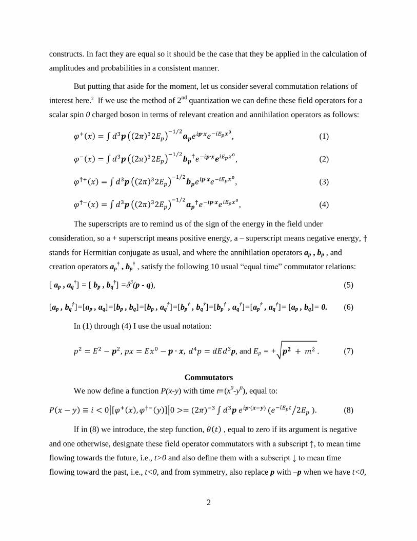
But putting that aside for the moment, let us consider several commutation relations of

interest here.2 If we use the method of 2nd

quantization we can define these field operators for a

scalar spin 0 charged boson in terms of relevant creation and annihilation operators as follows:

, (1)

, (2)

, (3)

, (4)

The superscripts are to remind us of the sign of the energy in the field under

consideration, so a + superscript means positive energy, a – superscript means negative energy,

stands for Hermitian conjugate as usual, and where the annihilation operators ap , bp , and

creation operators ap† , bp

† , satisfy the following 10 usual ―equal time‖ commutator relations:

[ ap , aq†] = [ bp , bq

†] =δ

3(p - q), (5)

[ap , bq†]=[ap , aq]=[bp , bq]=[bp , aq

†]=[bp

† , bq

†]=[bp

† , aq

†]=[ap

† , aq

†]= [ap , bq]= 0. (6)

In (1) through (4) I use the usual notation:

, p, and Ep = + . (7)

Commutators

We now define a function P(x-y) with time t≡(x0-y

0), equal to:

(8)

If in (8) we introduce, the step function, , equal to zero if its argument is negative

and one otherwise, designate these field operator commutators with a subscript ↑, to mean time

flowing towards the future, i.e., t>0 and also define them with a subscript ↓ to mean time

flowing toward the past, i.e., t<0, and from symmetry, also replace p with –p when we have t<0,

3

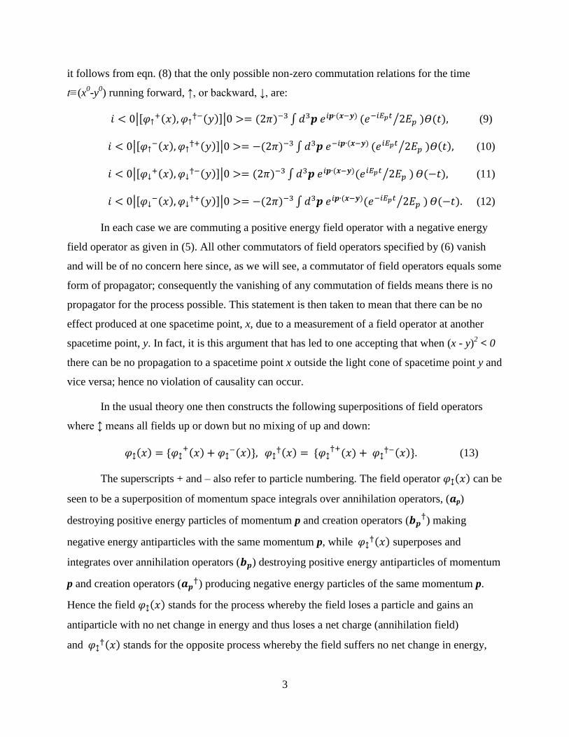
it follows from eqn. (8) that the only possible non-zero commutation relations for the time

t≡(x0-y

0) running forward, ↑, or backward, ↓, are:

(9)

(10)

(11)

(12)

In each case we are commuting a positive energy field operator with a negative energy

field operator as given in (5). All other commutators of field operators specified by (6) vanish

and will be of no concern here since, as we will see, a commutator of field operators equals some

form of propagator; consequently the vanishing of any commutation of fields means there is no

propagator for the process possible. This statement is then taken to mean that there can be no

effect produced at one spacetime point, x, due to a measurement of a field operator at another

spacetime point, y. In fact, it is this argument that has led to one accepting that when (x - y)2 < 0

there can be no propagation to a spacetime point x outside the light cone of spacetime point y and

vice versa; hence no violation of causality can occur.

In the usual theory one then constructs the following superpositions of field operators

where ↕ means all fields up or down but no mixing of up and down:

(13)

The superscripts + and – also refer to particle numbering. The field operator can be

seen to be a superposition of momentum space integrals over annihilation operators, ( p)

destroying positive energy particles of momentum p and creation operators ( ) making

negative energy antiparticles with the same momentum p, while superposes and

integrates over annihilation operators ( ) destroying positive energy antiparticles of momentum

p and creation operators ( ) producing negative energy particles of the same momentum p.

Hence the field stands for the process whereby the field loses a particle and gains an

antiparticle with no net change in energy and thus loses a net charge (annihilation field)

and stands for the opposite process whereby the field suffers no net change in energy,

4

loses an antiparticle, gains a particle and thus gains a net charge (creation process). If you

consider that antiparticles have the opposite charge of particles you can see that these fields

complement each other and also see that indeed they are Hermitian conjugates of each other.

One should notice that the direction of time is immaterial here but will become of interest

in what follows. Down arrow propagation works just as well as up arrow propagation. However

you can‘t superimpose or mix a down arrow field and an up arrow field.

Consequently, it is easy to show from (9) through (12) that:

(14)

Feynman propagators

It is useful to introduce the quantum field theoretical Feynman propagators for these

fields. I see these propagators as being more fundamental than the fields themselves. What

should be obvious is that no mention of the fields is even necessary and no mention of

antiparticles is necessary either, although this last consideration may seem less obvious.

Feynman‘s propagator approach is therefore, I believe, superior to the commutation of fields

approach for this reason: Feynman derives antiparticles from the particle propagators. Whereas

in the field commutation derivation, antiparticles must be postulated and then accepted.

Furthermore the antiparticle must have negative energies propagating forward through time and

when considering time running negatively, particles must have positive energy.

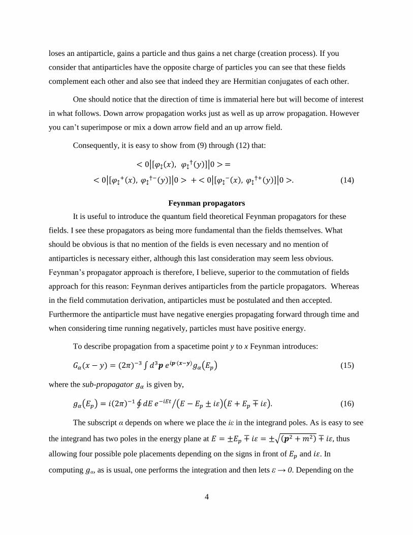
To describe propagation from a spacetime point y to x Feynman introduces:

(15)

where the sub-propagator is given by,

(16)

The subscript α depends on where we place the iε in the integrand poles. As is easy to see

the integrand has two poles in the energy plane at thus

allowing four possible pole placements depending on the signs in front of and . In

computing α, as is usual, one performs the integration and then lets ε → 0. Depending on the

5

placement of the poles with finite ε we find four possible sub-propagators in the limit ε → 0

given quite simply, again using t = (x0 – y

0):

ϴ(t), (17)

ϴ(-t), (18)

ϴ(t), (19)

ϴ(-t). (20)

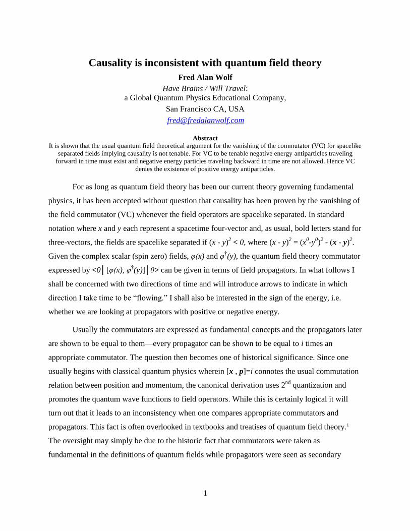
For simplicity in (17) through (20) I use the sub-index notation fl to stand for the

Feynman sub-propagator computed by closing the integration path in the lower half of the

complex energy plane (see Fig. 1) enclosing the positive energy pole, ), fu to stand for

closing the path in the upper half plane (see Fig. 2) enclosing the negative energy pole,

( ), and fl (Fig. 1) and fu (Fig. 2) correspondingly, what I call anti-Feynman sub-

propagators, representing closing the path in the lower or upper plane respectively but encircling

the opposite sign energy poles of fl, ( ), and of fu, ( ), resp.

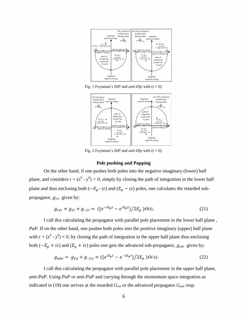
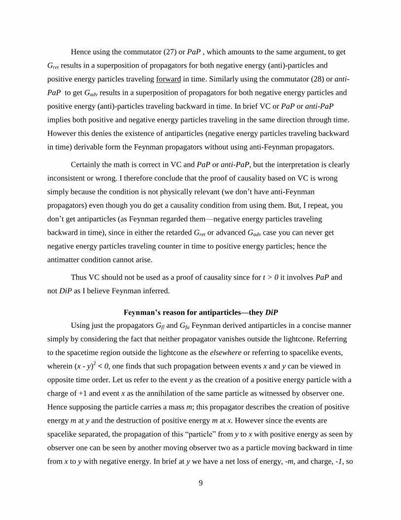
Pole pushing and Dipping

Feynman realized3 that one can push the two poles in (16) onto a diagonal alignment so

that the poles are placed at and or as we can see one could align the

poles along the anti-diagonal so that one has and I call calculating

the resulting sub-propagator with the first diagonal pole placement, DiP and the second anti-

diagonal pole placement anti-DiP. With DiP and carrying through the momentum space

integration as indicated in (15) one arrives at the Feynman propagators, Gfl and Gfu. While using

anti-DiP one gets the anti-Feynman propagators, G fl and G fu. In each case, with DiP or anti-

DiP, closing the integration path appropriately in either the upper or lower half plane, one gets

the residue from one pole only. Feynman only uses DiP in all calculations and never anti-DiP

which is the standard usage in calculating Feynman diagrams in quantum field theory texts to

date.4

6

Fig. 1 Feynman‘s DiP and anti-Dip with (t > 0).

Fig. 2 Feynman‘s DiP and anti-Dip with (t < 0).

Pole pushing and Papping

On the other hand, if one pushes both poles into the negative imaginary (lower) half

plane, and considers t = (x0 - y

0) > 0, simply by closing the path of integration in the lower half

plane and thus enclosing both ( – ) and ( ) poles, one calculates the retarded sub-

propagator, ret given by:

ϴ(t), (21)

I call this calculating the propagator with parallel pole placement in the lower half plane ,

PaP. If on the other hand, one pushes both poles into the positive imaginary (upper) half plane

with t = (x0 - y

0) < 0, by closing the path of integration in the upper half plane thus enclosing

both ( ) and ( ) poles one gets the advanced sub-propagator, adv given by:

ϴ(-t). (22)

I call this calculating the propagator with parallel pole placement in the upper half plane,

anti-PaP. Using PaP or anti-PaP and carrying through the momentum space integration as

indicated in (18) one arrives at the retarded Gret or the advanced propagator Gadv resp.

negative energy

positive energy

E=+E =

(p +m

p

+√ 2 2) -iε

-E=-E = (p +mp -√ 2 2) +iε

imaginary

positive energy

imaginary

negative energy

path of

integration

around the

+ pole Ep

DiP calculation

in Relativistic

Energy-plane

of Gfl

anti-DiP calculation

in Relativistic

Energy-plane

of G~fl

negative energy

positive energy

E=+E =

(p +m

p

+√ 2 2) +iε

path of

integration

around the

- pole Ep

-

E=-E =

(p +m

p

-√ 2 2) -iε

imaginary

positive energy

imaginary

negative energy

negative energy

positive energy

path of

integration

around the

- pole Ep

-E=+E =

(p +m

p

+√ 2 2) -iε

E=-E =

(p +m

p

-√ 2 2) +iε

imaginary

positive energy

imaginary

negative energy

DiP calculation

in Relativistic

Energy-plane

of Gfu

anti-DiP calculation

in Relativistic

Energy-plane

of G~fu

negative energy

positive energy

path of

integration

around the

pole Ep

-

E=+E =

(p +m

p

+√ 2 2) +iε

E=-E =

(p +m

p

-√ 2 2) -iε

imaginary

positive energy

imaginary

negative energy

7

Fig. 3. PaP and anti-PaP.

Relation of commutators with propagators

One can also easily calculate all of the Feynman propagators Gfl , Gfu , the anti-Feynman

propagators, G fl , G fu , and the retarded and advanced propagators Gret , Gadv , from the

commutation relations (9) through (12) and using (14). We find:

= = (23)

= (24)

= = (25)

= = (26)

(27)

. (28)

The usual reason people use (27) and (28) as proof of causality when (x - y)2 < 0, is that

both Gret and Gadv vanish, i.e., <0│[ (x), (y)]│0> = 0. This is easy to see using PaP. You

can see that ret and adv both vanish because you can Lorentz transform the spacelike interval

(x – y) to a coordinate system where t = (x0 - y

0) = 0. In so doing it is easy to see that

Gret = Gadv = 0, since from (21) with t = 0, we find = 0 and from (28) with t = 0, we

find = 0.

It is also easy to see that using PaP with t < 0, and enclosing the integration path in the

upper half plane that Gret = 0 simply because the integration path encloses no poles. A similar

argument holds for proving Gadv = 0 and enclosing the path in the lower half plane when t > 0.

PaP in the

Relativistic

Energy-plane

calaculation

negative energy positive energy

E=+E =

(p +m

p

+√ 2 2) -iε

path of

integration

around both

poles

-

E=-E =

(p +m

p

-√ 2 2) -iε

imaginary

positive energy

imaginary

negative energy

of Gret

negative energy positive energy

E=+E =

(p +m

p

+√ 2 2) +iε

path of

integration

around both

poles

-

E=-E =

(p +m

p

-√ 2 2) +iε

imaginary

positive energy

imaginary

negative energy

anti-PaP in the

Relativistic

Energy-plane

calaculation

of Gadv

8

Fig. 4 Simple PaP proof of causality.

Thus whenever the fields are spacelike separated the commutators and indeed

both vanish.5 Although this appears perfectly reasonable, the use of VC to argue for causality

inconsistently applies the Feynman and anti-Feynman propagators in the commutators defined in

(23) through (28). One uses both Feynman and anti-Feynman sub-propagators to calculate PaP

(and anti-PaP) and therefore assumes the superpositions of them valid. But this prescription is

invalid for a good reason— mixes negative energy particles (labeled as antiparticles using

commutators) propagating forward in time (24),with positive energy particles propagating

forward in time (23) and conversely mixes negative energy particles with

positive energy particles (26) both propagating backward in time. Hence the anti-Feynman

propagators are clearly not valid and should, therefore, not be used in any

commutation relations because they predict field operators yielding negative energy particles

forward in time or field operators yielding positive energy particles going backward in time.

With PaP and anti-PaP one must have the residues from both Feynman and anti-

Feynman poles contributing to the retarded and advanced propagators, resp. Feynman certainly

noticed this since he never used anti-Feynman propagators in his landmark papers.6 In fact he

argued for positive energy particles convincingly in Elementary Particles and the Laws of

Physics.7 Consequently we can safely infer that since if it is not wrong it is at least inconsistent to

use anti-Feynman sub-propagators, fl and fu in quantum field theory. PaP is invalid because

from (27) you have negative frequencies (energies) coming from fl contributing to the

propagator, Gret and similarly, from (28) using anti-PaP you have positive frequencies (energies)

coming from fu contributing to the propagator, Gadv regardless of the sign of (x - y)2.

simple PaP proof of causality in the

Relativistic Energy-plane: no poles

inside the closed path

negative energy positive energy

E=+E =

(p +m

p

+√ 2 2) -iε

path of

integration

around neither

pole

-

E=-E =

(p +m

p

-√ 2 2) -iε

imaginary

positive energy

9

Hence using the commutator (27) or PaP , which amounts to the same argument, to get

Gret results in a superposition of propagators for both negative energy (anti)-particles and

positive energy particles traveling forward in time. Similarly using the commutator (28) or anti-

PaP to get Gadv results in a superposition of propagators for both negative energy particles and

positive energy (anti)-particles traveling backward in time. In brief VC or PaP or anti-PaP

implies both positive and negative energy particles traveling in the same direction through time.

However this denies the existence of antiparticles (negative energy particles traveling backward

in time) derivable form the Feynman propagators without using anti-Feynman propagators.

Certainly the math is correct in VC and PaP or anti-PaP, but the interpretation is clearly

inconsistent or wrong. I therefore conclude that the proof of causality based on VC is wrong

simply because the condition is not physically relevant (we don‘t have anti-Feynman

propagators) even though you do get a causality condition from using them. But, I repeat, you

don‘t get antiparticles (as Feynman regarded them—negative energy particles traveling

backward in time), since in either the retarded Gret or advanced Gadv case you can never get

negative energy particles traveling counter in time to positive energy particles; hence the

antimatter condition cannot arise.

Thus VC should not be used as a proof of causality since for t > 0 it involves PaP and

not DiP as I believe Feynman inferred.

Feynman’s reason for antiparticles—they DiP

Using just the propagators Gfl and Gfu Feynman derived antiparticles in a concise manner

simply by considering the fact that neither propagator vanishes outside the lightcone. Referring

to the spacetime region outside the lightcone as the elsewhere or referring to spacelike events,

wherein (x - y)2 < 0, one finds that such propagation between events x and y can be viewed in

opposite time order. Let us refer to the event y as the creation of a positive energy particle with a

charge of +1 and event x as the annihilation of the same particle as witnessed by observer one.

Hence supposing the particle carries a mass m; this propagator describes the creation of positive

energy m at y and the destruction of positive energy m at x. However since the events are

spacelike separated, the propagation of this ―particle‖ from y to x with positive energy as seen by

observer one can be seen by another moving observer two as a particle moving backward in time

from x to y with negative energy. In brief at y we have a net loss of energy, -m, and charge, -1, so

10

the spacetime region around y carries both negative energy and negative charge in comparison

with its previous zero energy and charge status before event y occurred. Conversely the

spacetime region around event x would show a gain of positive charge +1 and a similar gain of

energy m.

While the 1st observer has no problem identifying the propagator for this process as a DiP

calculation of Gfl describing a positive energy particle going forward in time from y to x as seen

in the left side of Fig 1, the 2nd

observer would regard the same process as a DiP calculation of

Gfu describing a negative energy particle with negative charge -1 moving backward in time from

x to y as seen on the left side of Fig 2.

Hence we realize that while observer one sees the time of event y0 as occurring before the

time of event x0, ( x

0- y

0) > 0 , observer two sees the time of event y

0 as occurring after the time

of event x0, ( y

0- x

0) > 0. So observer two, seeing that the region around x now carries a net

positive charge of +1 and a positive energy m, would reason that some kind of ―particle‖ with

charge -1 and energy -m traveled from x to y thus accounting for the negative energy –m and

charge at y. Thus we have the discovery of antiparticles without resorting to introducing them via

extra creation and annihilation operators in the field description, ala the antiparticle creation

operator bp†

and destruction operator bp.

Hence the reason for antiparticles arises from elsewhere propagation as Feynman put it;

―one man‘s virtual particle is another man‘s virtual antiparticle.‖ Once we accept that elsewhere

propagation must occur we can reason appropriately using only propagators Gfl to describe

particles and Gfu to describe antiparticles even when the propagation is contained within the

lightcone of either particle or antiparticle. In brief, the Feynman prescription is universal—we

need not only consider elsewhere propagation. There is no need to invoke the anti-Feynman

propagators G fl and G fu. Using them introduces an inconsistency, e.g., G fl indicates a negative

energy particle traveling forward in time, G fu indicates a positive energy particle traveling

backward in time, and each is computed from the commutator of the antiparticle creation

operator bp†

and destruction operator bp as shown in (9). In the Feynman scheme there is no need

to include the creation bp†

and destruction bp operators.

11

Counter arguments

One can object to my conclusion based on various historical and accepted field

theoretical grounds. Let me consider a few. On p. 7 of ―The Conceptual Basis Of Quantum Field

Theory‖ by Gerard ‗t Hooft where in describing the use of the Green‘s function for calculating

propagators, he says: ―Our choice can be indicated by shifting the pole by an infinitesimal

imaginary number, after which we choose the contour C to be along the real axis of all

integrands.‖ Then he says that this prescription results in causality.8 I agree. However, he doesn‘t

mention that he is shifting two poles so that they are in PaP condition. Of course you get

causality and VC but I contend you don‘t have antiparticles since you don‘t have elsewhere

propagation and you must have the anti-Feynman propagators G fl and G fu. He further writes:

―This Green function, called the forward Green function, gives our expressions the

desired causality structure: There are obviously no effects that propagate backwards in time, or

indeed faster than light. The converse choice, . . . gives us the backward solution. However, in

the quantized theory, we will often be interested in yet another choice, the Feynman

propagator . . .‖

In Weinberg‘s book. ―The quantum theory of fields,‖ the question of what the VC can

mean using the Hamiltonian evaluated at two different spacelike separated points x and y, where

(x - y)2 < 0, in chapters 3 and 5 is considered.9 He uses the fact that [H(x), H(y)] = 0 where H is

the Hamiltonian, for spacelike fields. He writes on the last paragraph of p. 198, and I paraphrase:

―The . . .[commutator] conditions [based on commutation of fields] are plausible for

photon fields (ala Bohr and Rosenfeld), however we are dealing with fields like the Dirac field

that do not seem measurable . . . The point of view taken here is that . . . [ψ(x),ψ(y)]± = 0 (anti-

commutation or commutation) is needed for Lorentz invariance of the S-Matrix, without any

ancillary assumptions about measurability or causality.‖

I have not disputed this. In fact I have used Weinberg‘s observation. If you look through

his book, he is very careful to not, or to hardly, mention causality at all. He instead uses the term

―causal fields‖ throughout but that always means VC. On pp. 202-205, he recognizes in eq.

(5.2.6), the Feynman propagator, what he calls the Δ+(x) function, fails to vanish. I am not

disagreeing with Weinberg here. I am only pointing out that the approach that uses the VC is

inconsistent with the Feynman propagator point of view which seems to be valid. What surprises

12

me, and I really do not understand Weinberg here, is that by essentially denying the use of the

Feynman propagator scheme that I outline in the paper, he still argues that antiparticles exist.

Hence from Weinberg you apparently do have antiparticles in the KG (Klein-Gordon)

scalar field case and yet you exclude propagation into the elsewhere. I really don‘t understand

this. Oh, to be clear, elsewhere propagation is to me the same thing as (virtual) tachyons which

is the same thing as my invalidation point about VC (vanishing of the commutator). I think all

you really need for an antiparticle, and by implication elsewhere propagation, is for the particle

field to carry a charge—some form of interaction in the Lagrangian like iV.10

So in brief there is objection to tachyons in the KG case, however, this is counter to

Feynman‘s point of view.11 He consider tachyons, i.e., elsewhere propagation (that Weinberg

seems to deny) in the last part of his positron paper as I recall. He didn‘t use the term tachyon of

course—just propagation outside the lightcone (into the elsewhere).

One may also object on the grounds that the Feynman propagator is a c-number and

therefore not a measurable operator like a quantum field operator. Because the violations of

causality occur in the intermediate virtual states where one can also find other weird ―particles‖

emerging, it is natural to simply assume Feynman‘s method of calculating is just a mathematical

tool and only the results of measurement are important. Here we raise the question just what is

measurable in quantum field theory? It is usually supposed that VC implies measurability of the

fields in the commutator. The Feynman prescription of determining amplitudes from the

propagators that when squared appropriately to give probabilities and eventually cross sections,

seems to me to be measureable. So I don‘t see throwing Feynman‘s propagators out the window.

One also needs to consider that the propagators are equal to the commutators (multiplied by i).

One can also examine the question of the spin-statistics connection12 raised by Pauli and

his use of the commutator to make his point about spin ½ fields having anti-commuting fields

while spin 0,1, etc, must have commuting spacelike separated fields. Pauli‘s D function is in

effect calculated from integrating using (1). He also considers another function that

he calls D1 that is the same as integration of the linear combination . Pauli

recognizes that D1 leads to trouble and simply throws it out of consideration in his proofs. He

also never considers the time reversal sub-propagators . He wrote:

13

―The justification for our postulate lies in the fact that measurement at two space

points with a spacelike distance can never disturb each other, since no signals can be

transmitted with velocities greater than that of light. Theories which would make use of

the D1 function in their quantization would be very different from the known theories in

their consequences.13.

―Hence we come to the result (Italics Pauli‘s.): For integral spin the quantization

according to the exclusion principle is not possible. For this reason it is essential, that

the use of the D1 function in place of the D function be, for general reasons, discarded.‖ 14

By denying D1 one in effect denies the separability of into two functions

and . For with both D1 and D we can determine these Feynman and anti-Feynman

propagators (Green‘s functions) by simply adding or subtracting D1 and D. Hence Pauli throws

the baby (anti-causality) out with the bathwater (separation of the Feynman and anti-Feynman

propagators).

Conclusion

If you insist on VC as proof of causality, whereby nothing propagates into the elsewhere

when (x - y)2 < 0, you then must also insist that antimatter cannot exist and particles going

forward in time must have both positive and negative energies.15 This conclusion runs counter to

the usual 2nd

quantization method of quantum field theory. That is my point—the two are not

consistent. Since you can‘t have it both ways (PaP and DiP) and since we don‘t have negative

energy particles going forward in time and we do have antiparticles (negative energy particles

going backward in time16), you must only use DiP consistently. Thus the usual VC for spacelike

separated fields cannot be used even though it is mathematically true. Simply put, VC gives Gret

or Gadv constructed from anti-Feynman propagators which are invalid in quantum field theory.

Gret implies negative energy particles traveling forward in time and Gadv implies positive energy

particles traveling backward in time resulting in an unstable universe without the appearance of

antiparticles (negative energy particles traveling backward in time). It appears that one must give

up causality to gain antimatter and a stable universe.17

Acknowledgement

I would like to thank Jack Sarfatti and David Kaiser for helpful discussions and Waldyr

A. Rodrigues Jr. for a helpful correction.

14

1 There many such textbooks. I will only mention Weinberg, Steven. The Quantum Theory of Fields. NY:

Cambridge University Press, 1995, 2005.

2 A good source book and derivation of the relationship between the commutator and the propagator can be

found on line by Robert D. Klauber. http://www.quantumfieldtheory.info/ and

http://www.quantumfieldtheory.info/WhCh050x.pdf.

3 Feynman, R. P. ―The Theory of Positrons.‖ Phys. Rev. 76 (1949), p. 757.

4 See for example, Zee, Anthony. Quantum Field Theory in a Nutshell. Second Edition. NJ: Princeton

University Press, 2010 among many others.

5 In fact with (x - y)

2 < 0, you can show by Lorentz transforming to different observers that you can find

(x0 - y

0) to be positive, negative, or zero and thus with PaP you can prove the spacelike commutator vanishes very

simply by closing in the half plane that has no poles included (the closed path integral vanishes via the calculus of

residues).

6 Feynman, Richard P. and Steven Weinberg. Elementary Particles and the Laws of Physics: The 1986

Dirac Memorial Lectures. New York: Cambridge University Press, 1987. p. 7. Also see Feynman, R. P. ―The

Theory of Positrons.‖ Phys. Rev. 76 (1949), p. 757.

7 Feynman, Richard P. and Steven Weinberg. Ibid. p. 7.

8 ‗t Hooft, Gerard. ―The Conceptual Basis Of Quantum Field Theory‖ Handbook of the Philosophy of

Science, (2004). Also see (http://www.phys.uu.nl/~thooft/) for a complete list of publications.

9 Weinberg ibid.

10 See http://wiki.physics.fsu.edu/wiki/index.php/Klein-Gordon_equation for more on negative energy

states and antiparticles.

11 Feynman, R. P. ibid.

12 Pauli, W. ―The Connection Between Spin and Statistics.‖ Phys. Rev. 58, (1940), pp. 717-22. Also see

Sudarshan, E. C. G. The Fundamental Theorem on the Connection between Spin and Statistics, in Proc. Nobel

Symposium 8; Elementary Particle Theory, Relativistic Groups and Analyticity, Nils Svartholm (ed.), Almqvist and

Wiksell, Stockholm (1968), pp.379-386; and see Sudarshan, E. C. G. and Ian Duck Toward an Understanding of the

Spin-Statistics Theorem; Am. J. Phys. 66(4), 284 (1998).

13 See Pauli, W. p.721. Ibid.

14 See Pauli, W. p.722. Ibid.

15 We cannot have negative energy particles going forward in time because they would act as an energy

sink eventually swallowing up all positive energy particles. Similarly we cannot have positive energy particles

traveling backward in time for the same reason. Also see Sudarshan, E. C. G., The Nature of Faster than Light

Particles and Their Interactions, Arkiv. für Physik 39, 40 (1969).

16 Of course in this paper I am using the term ―going backward in time‖ as a calculation tool. Whether

particles actually do this is not subject to any experimental proof to date. All one needs to do is remember that a

negative energy particle moving backward in time with a negative charge would be seen by observers as a positive

15

energy particle moving forward in time with a positive charge and vice versa. Also see Sudarshan, E. C. G. and O.

M. P. Bilaniuk, Causality and Spacelike Signals;, Nature 223, 386 (1969).

17 Please see my book, Wolf, F. A. Time-loops and Space-twists: How God created the universe (San

Francisco, CA: Hampton Roads, Red Wheel Weiser, 2011) for a popular discussion of this topic and other concepts

from quantum field theory.