Department of Engineering ScienceUniversity of Oxford

CBT-TCS: the New Temperature and Soot

Loading Measurement Technique in a

Laminar Diffusion Flame

Huayong Zhao, Ben William, Richard Stone

Cambridge Particle Meeting 2011, 13th May 2011

Outline

Introduction

Experiment Setup and Software Packages

Accuracy Improvement Techniques

Sample Data and Assumptions

Conclusions

2

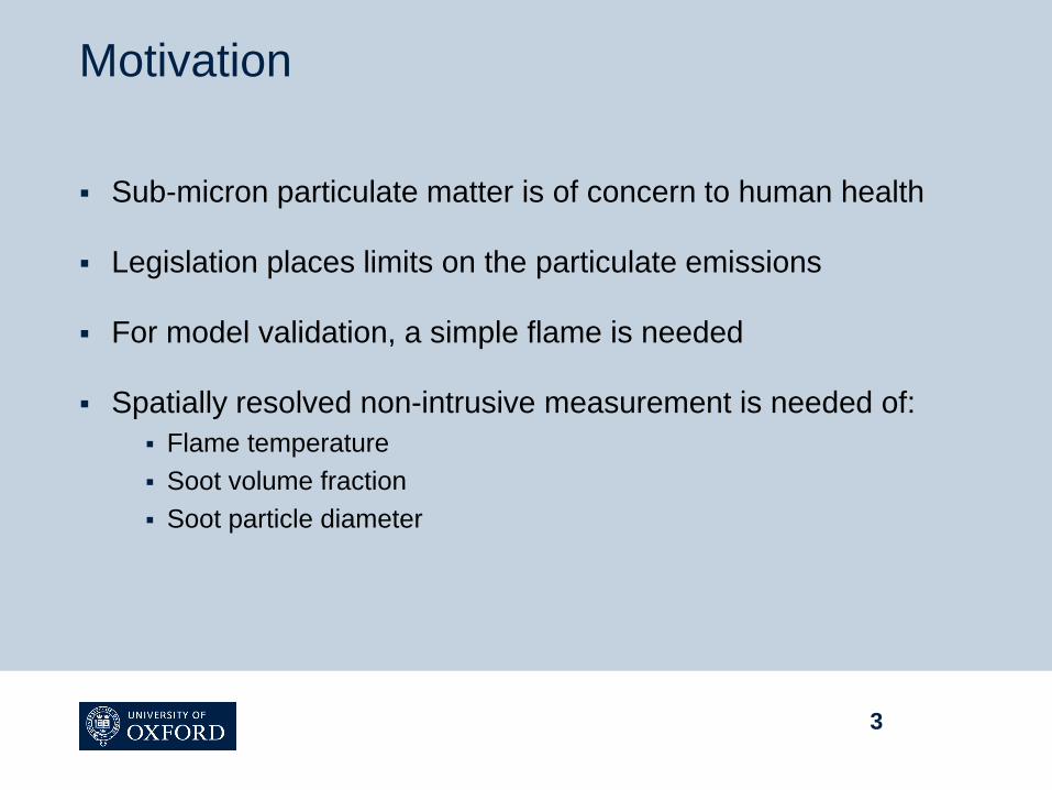
Motivation

Sub-micron particulate matter is of concern to human health

Legislation places limits on the particulate emissions

For model validation, a simple flame is needed

Spatially resolved non-intrusive measurement is needed of:

Flame temperature

Soot volume fraction

Soot particle diameter

3

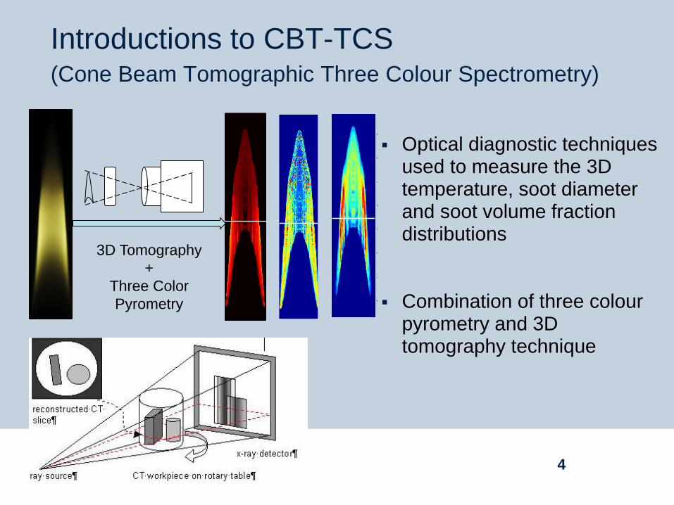
Introductions to CBT-TCS (Cone Beam Tomographic Three Colour Spectrometry)

Optical diagnostic techniques used to measure the 3D temperature, soot diameter and soot volume fraction distributions

Combination of three colour pyrometry and 3D tomography technique

4

Temperature (K)

y (cm)

z (cm)

-0.4-0.200.20.4

1.5

2

2.5

3

3.5

4

4.5

5

5.5

1500

1550

1600

1650

1700

1750

1800

1850

1900

1950

2000Diameter (micrometer)

y (cm)

z (cm)

-0.4-0.200.20.4

1.5

2

2.5

3

3.5

4

4.5

5

5.5

0

10

20

30

40

50

60

70

80

Soot Volume Fraction (ppm)

y (cm)

z (cm)

-0.4-0.200.20.4

1.5

2

2.5

3

3.5

4

4.5

5

5.5

20

40

60

80

100

120

140

160

180

200

3D Tomography

+

Three Color

Pyrometry

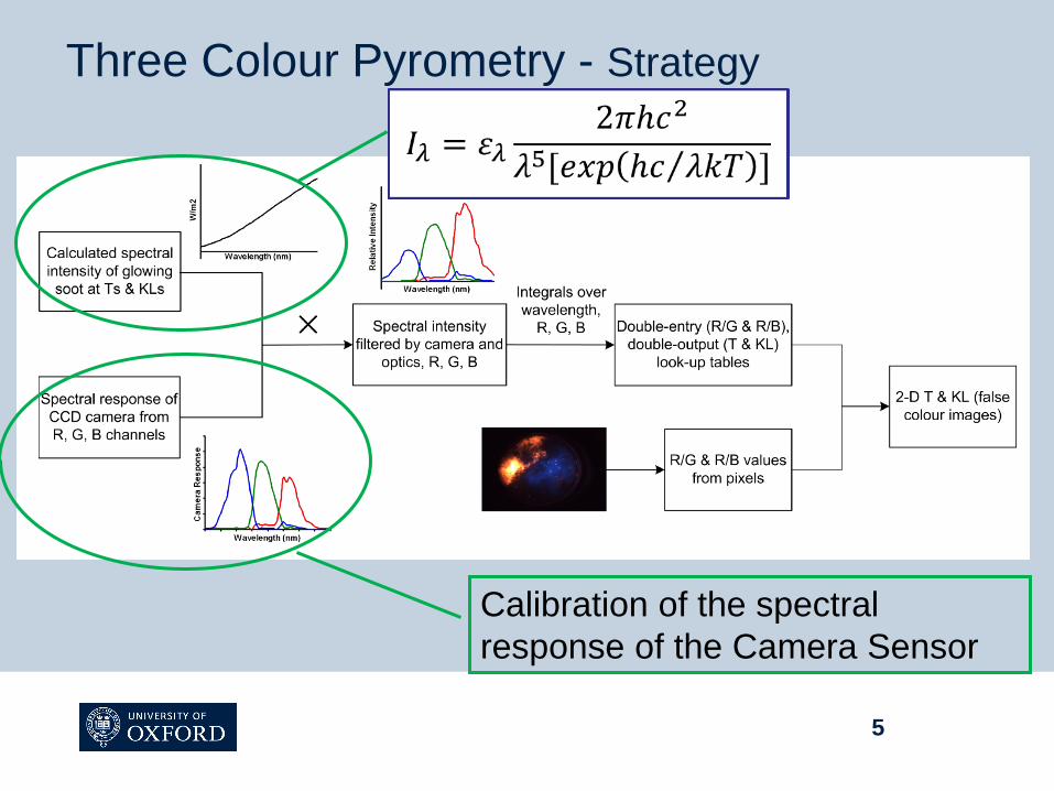
Three Colour Pyrometry - Strategy

5

Calibration of the spectral

response of the Camera Sensor

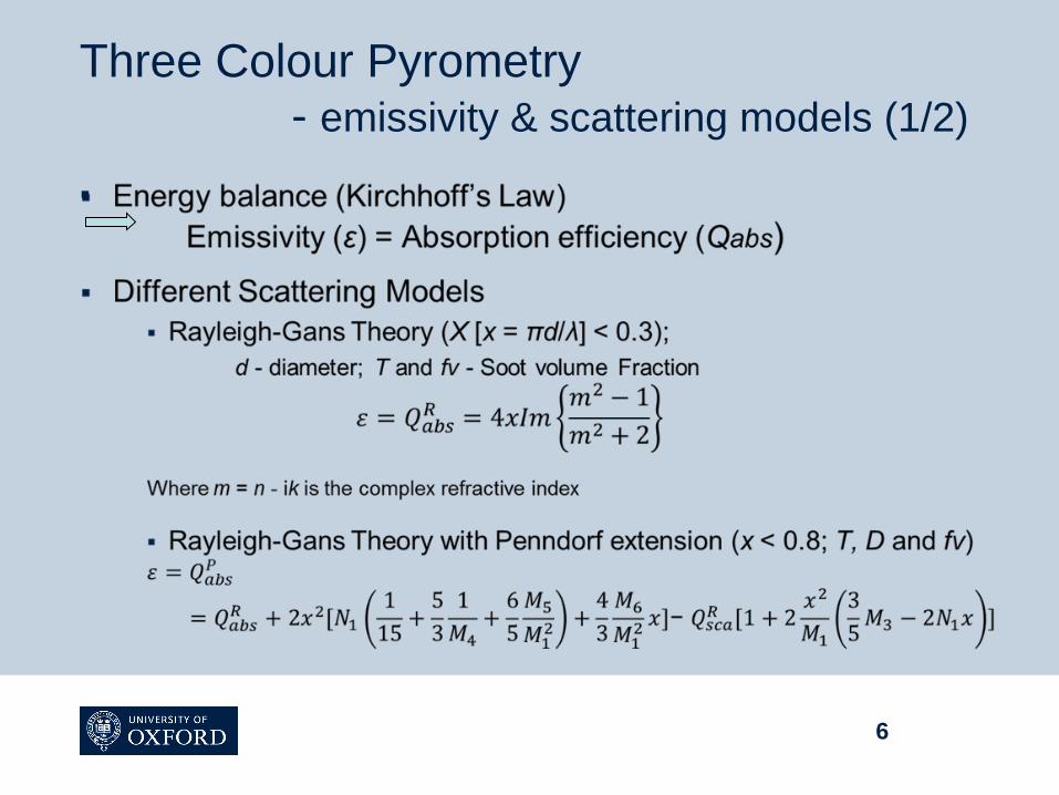
Three Colour Pyrometry - emissivity & scattering models (1/2)

6

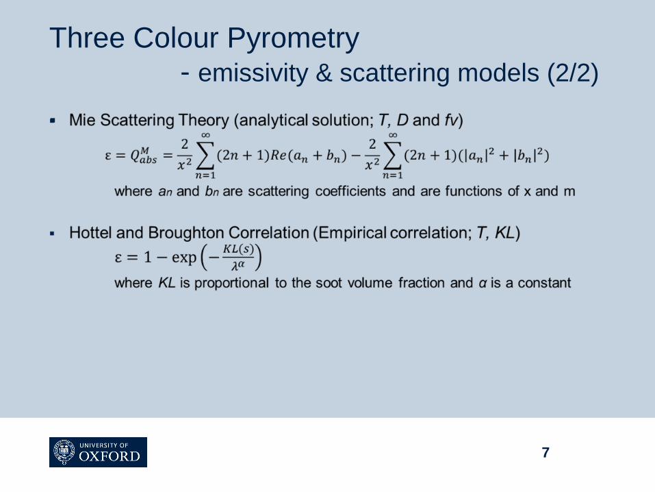
Three Colour Pyrometry - emissivity & scattering models (2/2)

7

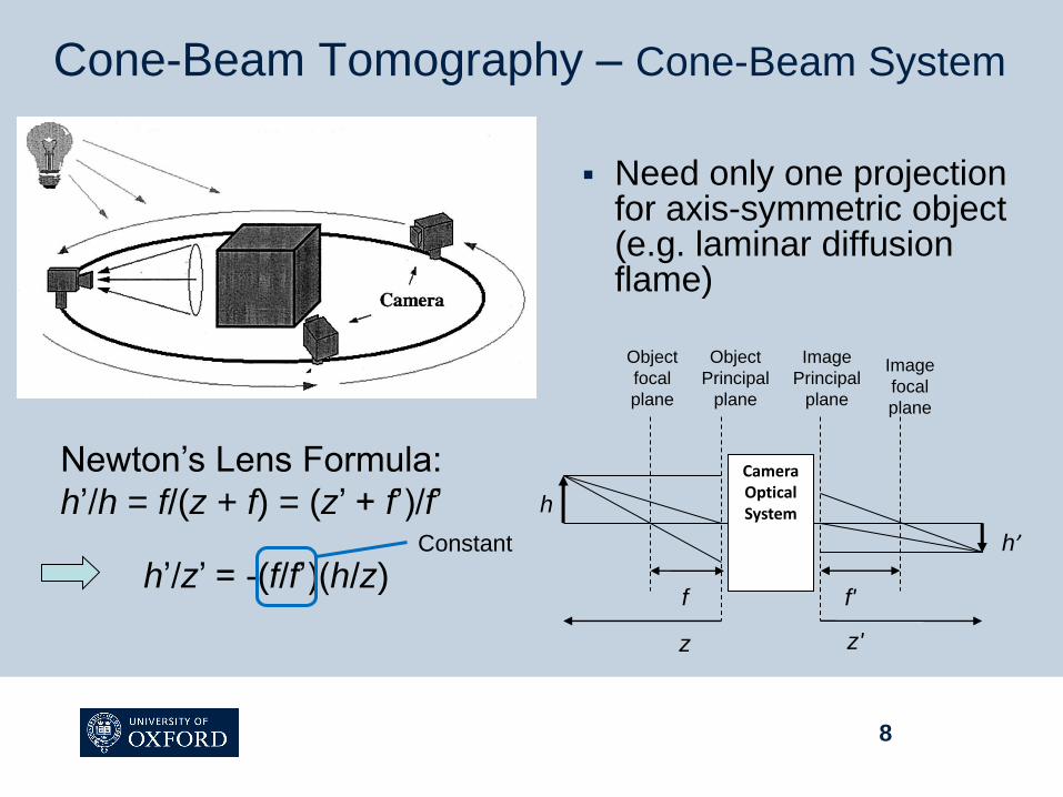
Cone-Beam Tomography – Cone-Beam System

Need only one projection for axis-symmetric object (e.g. laminar diffusion flame)

8

Camera Optical System

Image

focal

plane

Object

Principal

plane

Object

focal

plane

Image

Principal

plane

h

h’

f'

z'

f

z

Newton’s Lens Formula:

h’/h = f/(z + f) = (z’ + f’)/f’

h’/z’ = -(f/f’)(h/z)Constant

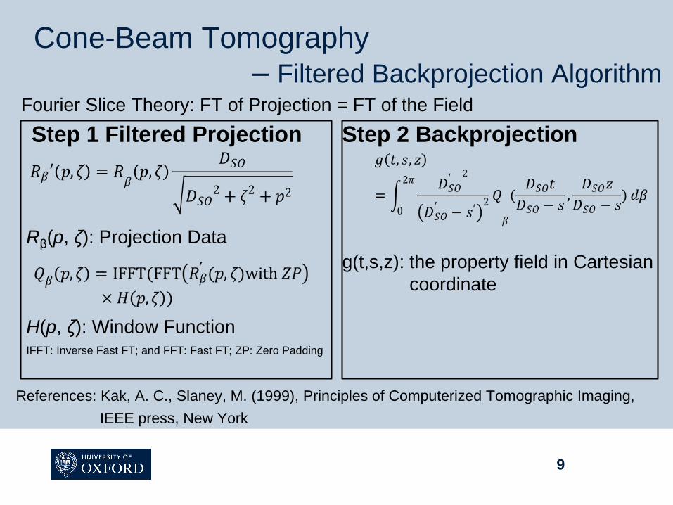
Cone-Beam Tomography – Filtered Backprojection Algorithm

Step 1 Filtered Projection

Rβ(p, ζ): Projection Data

H(p, ζ): Window FunctionIFFT: Inverse Fast FT; and FFT: Fast FT; ZP: Zero Padding

Step 2 Backprojection

g(t,s,z): the property field in Cartesian

coordinate

9

References: Kak, A. C., Slaney, M. (1999), Principles of Computerized Tomographic Imaging,

IEEE press, New York

Fourier Slice Theory: FT of Projection = FT of the Field

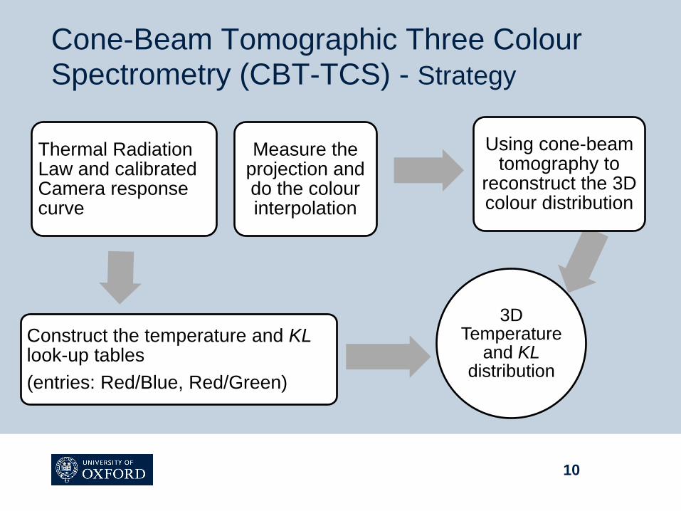
Cone-Beam Tomographic Three Colour Spectrometry (CBT-TCS) - Strategy

3D Temperature

and KLdistribution

Measure the projection and do the colour interpolation

Using cone-beam tomography to

reconstruct the 3D colour distribution

Construct the temperature and KLlook-up tables

(entries: Red/Blue, Red/Green)

Thermal Radiation Law and calibrated Camera response curve

10

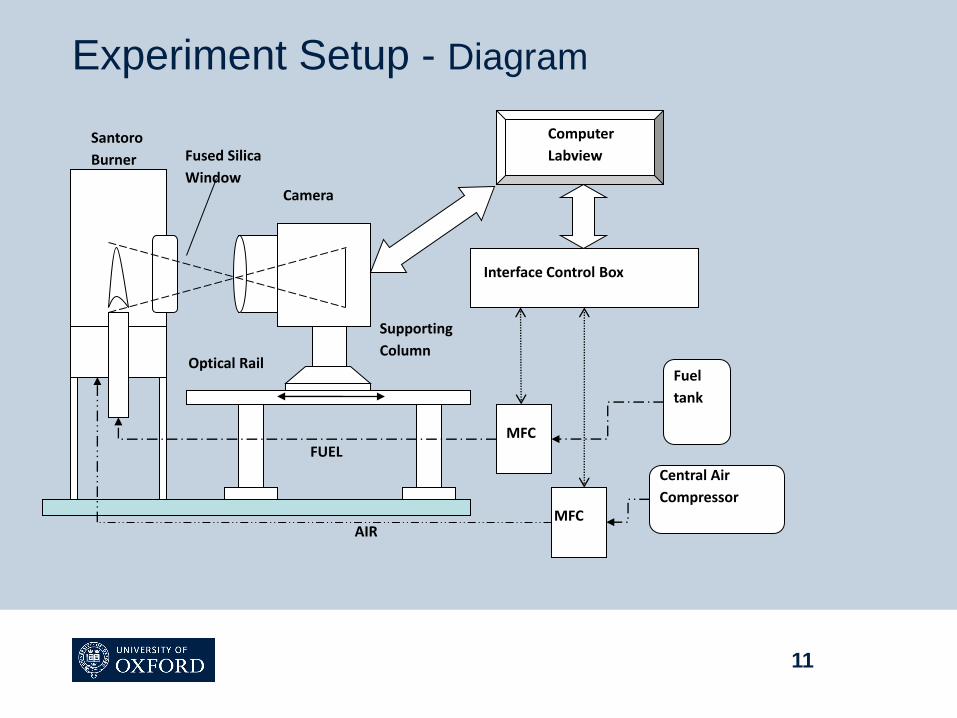
Experiment Setup - Diagram

11

Interface Control Box

MFC

MFC

Fuel

tank

Central Air

Compressor

AIR

FUEL

Santoro

Burner

Optical Rail

Camera

Supporting

Column

Fused Silica

Window

Computer

Labview

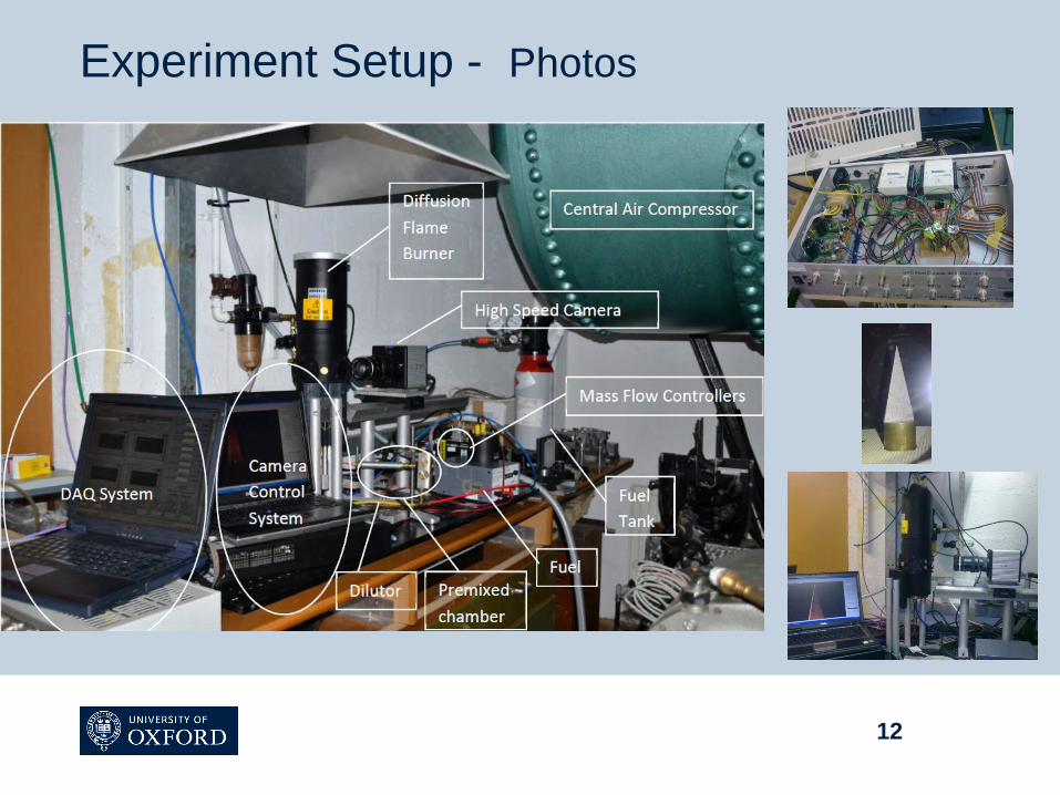
Experiment Setup - Photos

12

Open source tomography code

OSCaR source code URL: www.cs.toronto.edu/~urezvani/OSCaR.html

Three MATLAB GUIs

Functions of original code:

Predefine parameters to do the tomography

Implementing the 3D filtered backprojection algorithm to X-ray images from different gantry

angles by using different window functions

Software Package – Original OSCaR

13

Open source tomography code

OSCaR source code URL: www.cs.toronto.edu/~urezvani/OSCaR.html

Three MATLAB GUIs

Functions of original code:

Predefine parameters to do the tomography

Implementing the 3D filtered backprojection algorithm to X-ray images from different gantry

angles by using different window functions

Software Package – Original OSCaR

13

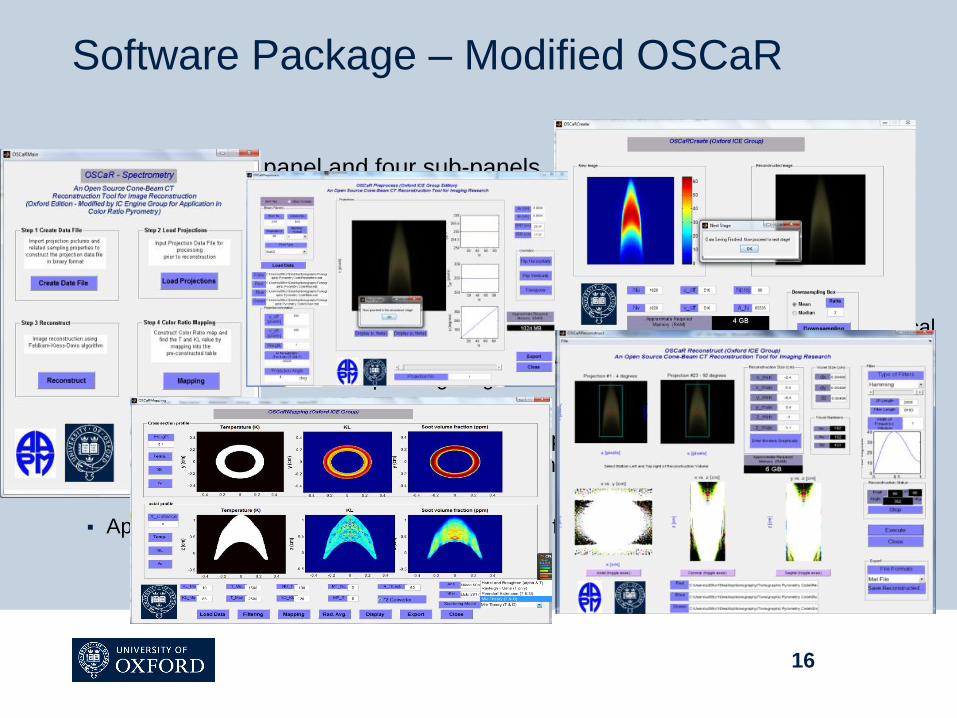
Including one main panel and four sub-panels

Extended functions:

Read projection images, do the colour demosaicing and the downsampling

Modified the 3D filtered backprojection algorithm to make it applicable to current optical

setup and apply this algorithm to individual colour channels by using different window

functions with different zero-padding lengths

Applying 3D median filter, construct the look-up table and do the mapping to find T, D

and fv according to the selected optical components and scattering model

Apply a circumferential average and export the final data matrix

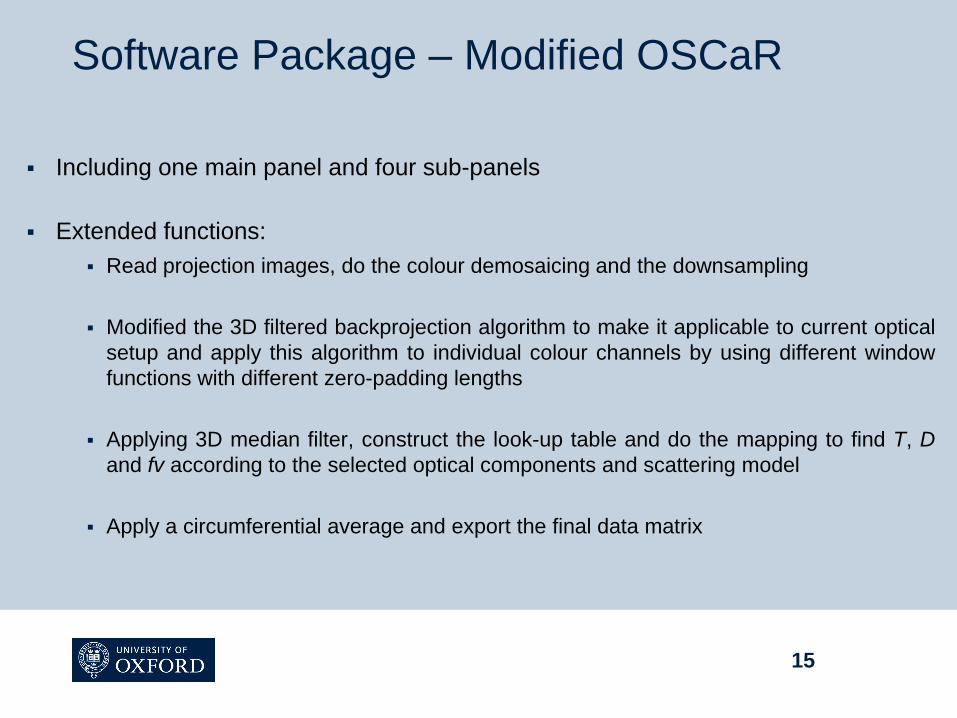
Software Package – Modified OSCaR

15

Including one main panel and four sub-panels

Extended functions:

Read projection images, do the colour demosaicing and the downsampling

Modified the 3D filtered backprojection algorithm to make it applicable to current optical

setup and apply this algorithm to individual colour channels by using different window

functions with different zero-padding lengths

Applying 3D median filter, construct the look-up table and do the mapping to find T, D

and fv according to the selected optical components and scattering model

Apply a circumferential average and export the final data matrix

Software Package – Modified OSCaR

16

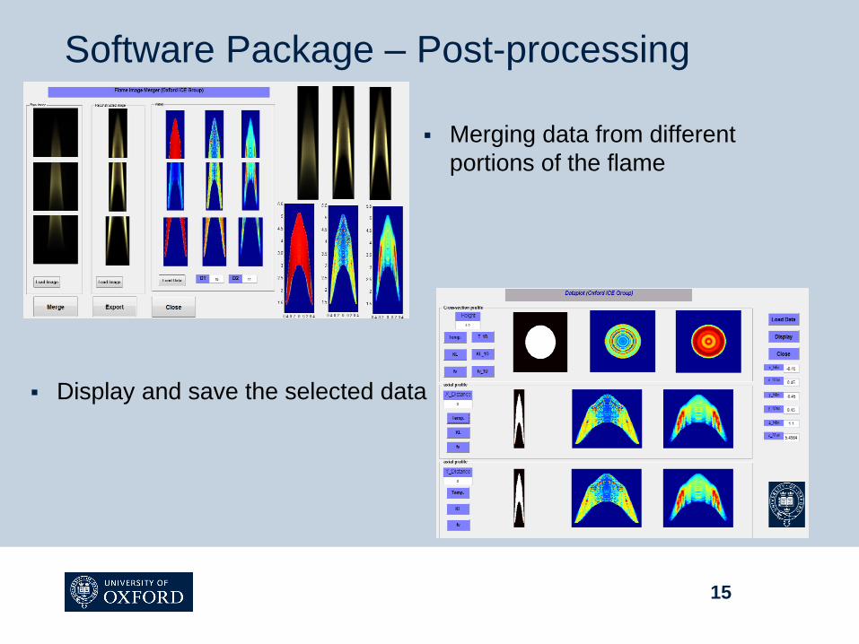
Software Package – Post-processing

15

Merging data from different

portions of the flame

Display and save the selected data

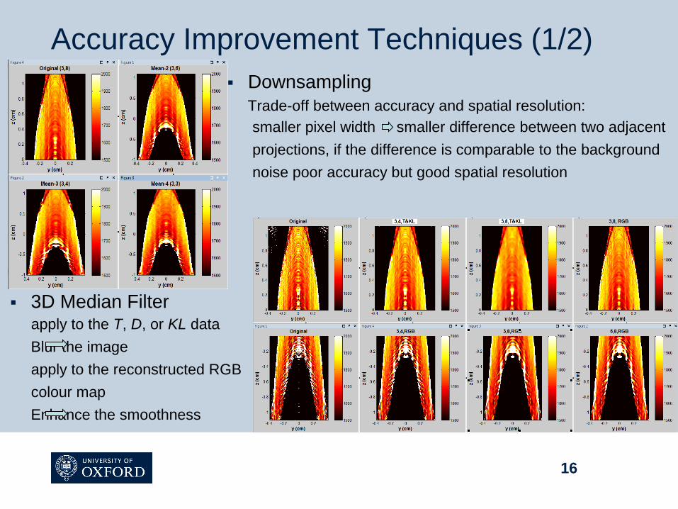
Accuracy Improvement Techniques (1/2)

Downsampling

Trade-off between accuracy and spatial resolution:

smaller pixel width smaller difference between two adjacent

projections, if the difference is comparable to the background

noise poor accuracy but good spatial resolution

3D Median Filterapply to the T, D, or KL data

Blur the image

apply to the reconstructed RGB

colour map

Enhance the smoothness

16

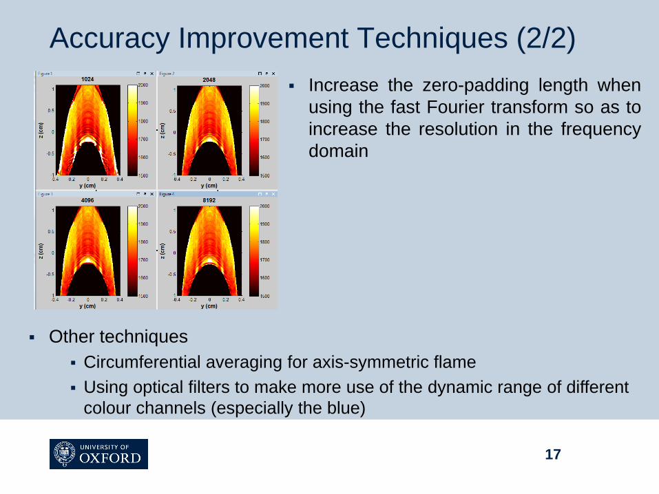
Accuracy Improvement Techniques (2/2)

Increase the zero-padding length when

using the fast Fourier transform so as to

increase the resolution in the frequency

domain

Other techniques

Circumferential averaging for axis-symmetric flame

Using optical filters to make more use of the dynamic range of different

colour channels (especially the blue)

17

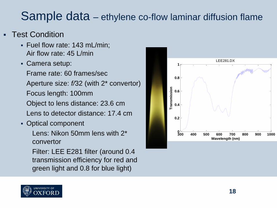
Sample data – ethylene co-flow laminar diffusion flame

18

Test Condition

Fuel flow rate: 143 mL/min;

Air flow rate: 45 L/min

Camera setup:

Frame rate: 60 frames/sec

Aperture size: f/32 (with 2* convertor)

Focus length: 100mm

Object to lens distance: 23.6 cm

Lens to detector distance: 17.4 cm

Optical component

Lens: Nikon 50mm lens with 2*

convertor

Filter: LEE E281 filter (around 0.4

transmission efficiency for red and

green light and 0.8 for blue light)

300 400 500 600 700 800 900 10000

0.2

0.4

0.6

0.8

1LEE281.DX

Wavelength (nm)

Tra

ns

mis

sio

n

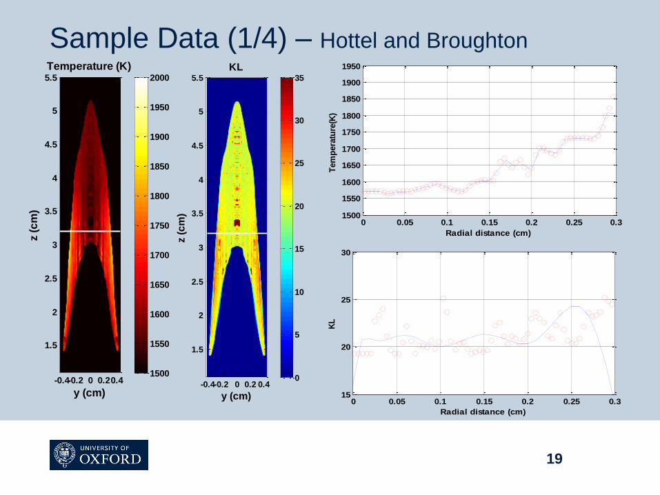
Sample Data (1/4) – Hottel and Broughton

19

Temperature (K)

y (cm)

z (

cm

)

-0.4-0.2 0 0.20.4

1.5

2

2.5

3

3.5

4

4.5

5

5.5

1500

1550

1600

1650

1700

1750

1800

1850

1900

1950

2000KL

y (cm)

z (

cm

)

-0.4-0.2 0 0.2 0.4

1.5

2

2.5

3

3.5

4

4.5

5

5.5

0

5

10

15

20

25

30

35

0 0.05 0.1 0.15 0.2 0.25 0.315

20

25

30

Radial distance (cm)

KL

0 0.05 0.1 0.15 0.2 0.25 0.31500

1550

1600

1650

1700

1750

1800

1850

1900

1950

Radial distance (cm)

Tem

pera

ture

(K)

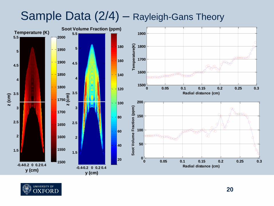
Sample Data (2/4) – Rayleigh-Gans Theory

20

Temperature (K)

y (cm)

z (

cm

)

-0.4-0.2 0 0.2 0.4

1.5

2

2.5

3

3.5

4

4.5

5

5.5

1500

1550

1600

1650

1700

1750

1800

1850

1900

1950

2000

Soot Volume Fraction (ppm)

y (cm)

z (

cm

)

-0.4-0.2 0 0.2 0.4

1.5

2

2.5

3

3.5

4

4.5

5

5.5

20

40

60

80

100

120

140

160

180

0 0.05 0.1 0.15 0.2 0.25 0.31500

1600

1700

1800

1900

Radial distance (cm)

Tem

pera

ture

(K)

0 0.05 0.1 0.15 0.2 0.25 0.30

50

100

150

200

Radial distance (cm)

So

ot

Vo

lum

e F

racti

on

(p

pm

)

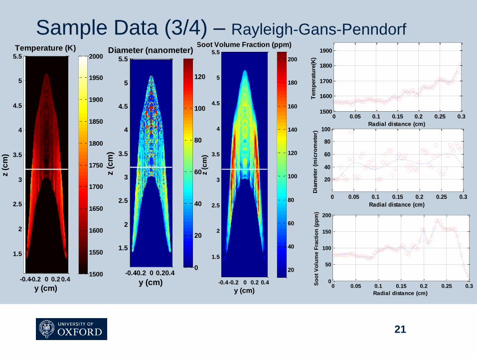
Sample Data (3/4) – Rayleigh-Gans-Penndorf

21

Temperature (K)

y (cm)

z (

cm

)

-0.4-0.2 0 0.2 0.4

1.5

2

2.5

3

3.5

4

4.5

5

5.5

1500

1550

1600

1650

1700

1750

1800

1850

1900

1950

2000

Soot Volume Fraction (ppm)

y (cm)

z (

cm

)

-0.4-0.2 0 0.2 0.4

1.5

2

2.5

3

3.5

4

4.5

5

5.5

20

40

60

80

100

120

140

160

180

200

0 0.05 0.1 0.15 0.2 0.25 0.31500

1600

1700

1800

1900

Radial distance (cm)

Tem

pera

ture

(K)

0 0.05 0.1 0.15 0.2 0.25 0.3

20

40

60

80

100

Radial distance (cm)

Dia

mete

r (m

icro

mete

r)

0 0.05 0.1 0.15 0.2 0.25 0.30

50

100

150

200

Radial distance (cm)

So

ot

Vo

lum

e F

racti

on

(p

pm

)

Diameter (nanometer)

y (cm)

z (

cm

)

-0.4-0.2 0 0.20.4

1.5

2

2.5

3

3.5

4

4.5

5

5.5

0

20

40

60

80

100

120

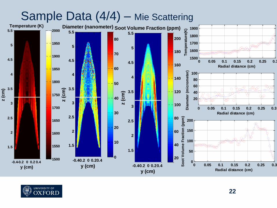
Sample Data (4/4) – Mie Scattering

22

Temperature (K)

y (cm)

z (

cm

)

-0.4-0.2 0 0.2 0.4

1.5

2

2.5

3

3.5

4

4.5

5

5.5

1500

1550

1600

1650

1700

1750

1800

1850

1900

1950

2000Soot Volume Fraction (ppm)

y (cm)

z (

cm

)

-0.4-0.2 0 0.20.4

1.5

2

2.5

3

3.5

4

4.5

5

5.5

20

40

60

80

100

120

140

160

180

200

0 0.05 0.1 0.15 0.2 0.25 0.31500

1600

1700

1800

1900

Radial distance (cm)

Tem

pera

ture

(K)

0 0.05 0.1 0.15 0.2 0.25 0.3

20

40

60

80

100

Radial distance (cm)

Dia

mete

r (m

icro

mete

r)

0 0.05 0.1 0.15 0.2 0.25 0.30

50

100

150

200

Radial distance (cm)

So

ot

Vo

lum

e F

racti

on

(p

pm

)

Diameter (nanometer)

y (cm)

z (

cm

)

-0.4-0.2 0 0.20.4

1.5

2

2.5

3

3.5

4

4.5

5

5.5

0

10

20

30

40

50

60

70

80

Assumptions (1/2)

Particulate temperature is the same as local flame

temperature

Thermal radiation from other species are negligible

compared to soot particles

CO2: 2.0, 2.7, 4.3, 9.4, 10.4 and 15 µm

H2O: 1.38, 1.87, 2.7, and 6.3 µm

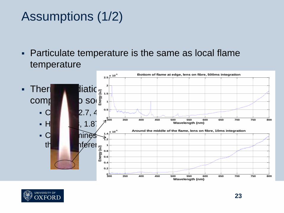
Chemilluminescence from radicals is negligible except from

the circumferential base of the flame

23

Assumptions (1/2)

Particulate temperature is the same as local flame

temperature

Thermal radiation from other species are negligible

compared to soot particles

CO2: 2.0, 2.7, 4.3, 9.4, 10.4 and 15 µm

H2O: 1.38, 1.87, 2.7, and 6.3 µm

Chemilluminescence from radicals is negligible except from

the circumferential base of the flame

23

300 350 400 450 500 550 600 650 700 750 8000

0.5

1

1.5

2

2.5x 10

-5 Bottom of flame at edge, lens on fibre, 500ms integration

Wavelength (nm)

Ene

rgy

(uJ)

300 350 400 450 500 550 600 650 700 750 8000

0.2

0.4

0.6

0.8

1

1.2

1.4x 10

-5 Around the middle of the flame, lens on fibre, 10ms integration

Wavelength (nm)

Ene

rgy

(uJ)

Assumptions (2/2)

The radiation attenuation along the optical path

is negligible (optical-thin approximation)

Not clear at this point

Can be partially corrected by using an iterative method suggested by

Lu et al. (2009)

Need to be corrected by introducing certain scattering models in the

future

24

Conclusions

The CBT-TCS technique is an effective and convenient opticaldiagnostic method to measure the spatially distributed temperature,soot diameters and soot volume fraction for an axi-symmetric flame

The optical-thin assumption may need to be addressed in the futureto increase its accuracy

CBT-TCS can be applied to asymmetric flames by using multipleimages

28