Comprehensive Capital Analysis and Review 2012:

Methodology for Stress Scenario Projections

March 12, 2012

B O A R D O F G O V E R N O R S O F T H E F E D E R A L R E S E R V E S Y S T E M

[blank page]

Comprehensive Capital Analysis and Review 2012:

Methodology for Stress Scenario Projections

March 12, 2012

B O A R D O F G O V E R N O R S O F T H E F E D E R A L R E S E R V E S Y S T E M

I. Introduction and Executive Summary

The Federal Reserve expects large, complex bank holding companies to hold sufficient capital to

maintain access to funding, to continue to serve as credit intermediaries, to meet their obligations to

creditors and counterparties, and to continue operations, even under adverse economic conditions. The

Comprehensive Capital Analysis and Review (CCAR) is a supervisory assessment by the Federal Reserve

of the capital planning processes and capital adequacy of these large, complex bank holding companies

(BHCs). The CCAR is the Federal Reserve's central mechanism for developing supervisory assessments of

capital adequacy at these firms.

Nineteen BHCs were required to participate in this year's CCAR (CCAR 2012).

[footnote] 1

The BHCs that participated in CCAR 2012 are Ally Financial Inc., American Express Company, Bank of America Corporation, The Bank of New York Mellon Corporation, BB&T Corporation, Capital One Financial Corporation, Citigroup Inc., Fifth Third Bancorp, The Goldman Sachs Group, Inc., JPMorgan Chase & Co., Keycorp, MetLife, Inc., Morgan Stanley, The PNC Financial Services Group, Inc., Regions Financial Corporation, State Street Corporation, SunTrust Banks, Inc., U.S. Bancorp, and Wells Fargo & Company. [end of footnote 1.]

In early January,

these BHCs submitted comprehensive capital plans to the Federal Reserve, describing their strategies for

managing their capital over a nine-quarter planning horizon. The purpose of requiring BHCs to develop

and maintain these capital plans is to ensure that the institutions have robust, forward-looking capital

planning processes that account for their unique risks and that the institutions have sufficient capital to

continue operations throughout times of economic and financial market stress. As part of its

assessment of the plans, the Federal Reserve projected losses, revenues, expenses, and capital ratios for

each of the 19 BHCs under a severely adverse macroeconomic scenario specified by the Federal Reserve.

This paper describes this scenario and provides an overview of the analytical framework and empirical

methods used by the Federal Reserve to generate these stress scenario projections.

The projections provide a unique perspective on the robustness of the capital positions of these

firms, because they incorporate detailed information about the risk characteristics and business

activities of each BHC and because they are estimated using a consistent approach across all of the

BHCs. The Federal Reserve is disclosing the stress scenario projections to enhance transparency about

the capital of the 19 BHCs participating in the CCAR exercise. The Federal Reserve also believes that

providing information about both the results of the stress scenario projections and the methodology will

provide useful context for market participants, analysts, academics, and others to interpret the results.

The stress scenario projections were calculated by Federal Reserve analysts using input data

provided by the 19 BHCs and a set of models developed or selected by the Federal Reserve. The

projections are based on a hypothetical, severely adverse macroeconomic and financial market scenario

developed by the Federal Reserve, featuring a deep recession in the United States, significant declines in

asset prices and increases in risk premia, and a slowdown in global economic activity (the "Supervisory

Stress Scenario"). Six BHCs with large trading, private equity, and derivatives activities are also subject

to a global financial market shock on those positions.

[footnote] 2 These BHCs are Bank of America Corporation, Citigroup Inc., The Goldman Sachs Group, Inc., JPMorgan Chase & Co., Morgan Stanley, and Wells Fargo & Company. [end of footnote 2.]

The Federal Reserve's projections for the 19 BHCs under the Supervisory Stress Scenario should

not be interpreted as expected or likely outcomes for these firms, but rather as possible results under

hypothetical, highly adverse conditions. The projections incorporate a number of conservative modeling

assumptions. The projections embed the capital actions - issuance of capital instruments, dividend

payments, and share repurchases - each BHC included in its capital plan under a baseline scenario

reflecting expected economic conditions. That is, BHCs are assumed to make their planned dividends

and other capital distributions even under the adverse conditions of the Supervisory Stress Scenario.

This conservative approach asks if a BHC would be able to meet supervisory expectations for capital

ratios should adverse economic conditions emerge and the BHC maintained its planned baseline

distributions. To illustrate the impact of the stress scenario alone, the Federal Reserve also calculated

stressed regulatory capital ratios excluding planned capital actions after Q1 2012.

[footnote] 3 The ratios assume planned capital actions through Q1 2012, but no material capital issuances from March 16 through March 31, 2012. [end of footnote 3.]

Finally, it is

important to note that the stress scenario projections estimate the impact of adverse economic and

financial market conditions on each institution's capital resources. The stress scenario projections do

not make explicit behavioral assumptions about the possible actions of a BHCs' creditors and

counterparties in the scenario, except through the Supervisory Stress Scenario's characterizations of

financial asset prices and economic activity.

II. Comprehensive Capital Analysis and Review

The CCAR is the central element of the Federal Reserve's approach to ensuring that large BHCs

have thorough and robust processes for managing their capital resources, supported by effective risk-

measurement and -management practices. In the first CCAR, conducted in early 2011, 19 large, complex

BHCs submitted comprehensive capital plans to the Federal Reserve, describing their strategies for

managing their capital over a nine-quarter planning horizon, and the Federal Reserve evaluated these

submissions.

[footnote] 4 See Board of Governors of the Federal Reserve System, "Comprehensive Capital Analysis and Review: Objectives and Overview" (March 18, 2011) for a full description of the 2011 CCAR. This paper is available at http://www.federalreserve.gov/newsevents/press/bcreg/bcreg20110318a1.pdf. [end of footnote 4.]

These 19 BHCs are the same institutions that participated in the 2009 Supervisory Capital

Assessment Program (SCAP).

[footnote] 5 See http://www.federalreserve.gov/bankinforeg/scap.htm for a description of the Supervisory Capital Assessment Program (SCAP). [end of footnote 5.]

In November 2011, the Federal Reserve issued a final rule requiring all U.S.-domiciled, top-tier

BHCs with consolidated assets of $50 billion or more to develop and submit capital plans to the Federal

Reserve on an annual basis (the capital plans rule).

[footnote] 6 76 Fed. Reg. 74631 (Dec. 1, 2011), to be codified at 12 CFR 225.8; see http://www.federalreserve.gov/newsevents/press/bcreg/20111122a.htm for a description of the capital plans rule. Until July 21, 2015, the capital plans rule will not apply to any BHC subsidiary of a foreign banking organization that is currently relying on Supervision and Regulation Letter SR 01-01 issued by the Board (as in effect on May 19, 2010). [end of footnote 6.]

This rule applies currently to 30 BHCs. CCAR 2012

focused on evaluation and assessment of the capital plans submitted by the 19 BHCs that participated in

the 2011 CCAR, while the capital plans of the additional 11 BHCs subject to the capital plans rule were

evaluated in a separate process (see the box on page 6).

Consistent with the capital plans rule, the Federal Reserve's analysis of these plans focused on

four key areas:

• the comprehensiveness of the capital plan, including the extent to which the analysis underlying

the plan captured and appropriately addressed potential risks stemming from all activities

across the BHC under baseline and stressed economic conditions;

• the reasonableness of the BHC's assumptions and analysis underlying the capital plan and the

robustness of its capital planning process;

• the BHC's capital policy governing distributions and other capital actions; and

• the BHC's ability to maintain capital above specified minimum regulatory capital ratios and

above a ratio of tier 1 common capital to risk-weighted assets of 5 percent

[footnote] 7 The 5 percent minimum for the tier 1 common ratio is a supervisory assessment (derived from an analysis of historical data for large U.S. BHCs) of how much common equity these firms need to provide a high degree of confidence that they could withstand unexpected future losses. [end of footnote 7.]

under both

expected conditions and stressful conditions throughout the planning horizon.

This last assessment was based on projections of each BHC's losses, revenue, expenses, and

capital ratios made by the BHCs and, separately, by the Federal Reserve. Each BHC made four sets of

projections under one baseline and one stress scenario developed by each firm ("BHC scenarios") and

one baseline and one stress scenario developed by the Federal Reserve ("supervisory scenarios").

[footnote] 8 Some BHCs opted to use the Supervisory Baseline Scenario as their own baseline scenario, and thus made only three sets of projections. [end of footnote 8.]

As part of its review of the capital plans, the Federal Reserve generated its own projections of

the BHCs' losses, revenues, expenses, and capital ratios under severely adverse economic and financial

market conditions. These stress scenario projections are based on data provided by the BHCs in

regulatory reports and models developed by Federal Reserve staff, applied in a consistent manner

across all BHCs. By examining all 19 BHCs simultaneously, the Federal Reserve was able to enhance its

institution-specific analysis with information about peers, applying consistent assumptions and bringing

a cross-firm perspective. For these reasons, the Federal Reserve's projections would be expected to

differ from the BHCs' projections of their own performance under the same set of hypothetical adverse

conditions and with projections made by outside analysts.

The Federal Reserve will notify each BHC of whether or not the Federal Reserve has any

objection to its capital plan or to the planned capital distributions in the plan.

[footnote] 9 In CCAR 2012, BHCs will receive this notification by March 15, 2012. [end of footnote 9.]

BHCs are required to

update and re-submit their capital plans within 30 days if the Federal Reserve objects to the plan or at

any time before the next CCAR exercise if the BHC or the Federal Reserve determines that there has

been a material change in the firm's risk profile, financial condition, or corporate structure. If the

Federal Reserve objects to a capital plan, a BHC may not make any capital distributions unless the

Federal Reserve specifically indicates it does not object to the distribution.

[footnote] 10 12 CFR 225.8(d)(4). [end of footnote 10.]

The Federal Reserve may

object to all distributions described in the plan, or just to some.

The decision to object or not object to a BHC's capital plan rests on the full range of capital plan

elements evaluated by the Federal Reserve. One or more of a BHC's capital plan elements could be

strong, but the Federal Reserve might still object to the firm's plan based on unacceptable performance

on one or more of the other elements. The Federal Reserve assessed each BHC's capital planning

processes, the governance structure guiding those processes, the risk measurement and management

systems supporting these processes, as well as assessments of whether each BHC is making steady

progress to meet regulatory capital standards agreed to by the Basel Committee on Banking Supervision

("Basel III") as they would come into effect in the United States over time. The BHC's and Federal

Reserve's projections of losses, revenue, expenses, and capital under stressed economic conditions -

the stress scenario projections - are a critical part of this decision, but not the only consideration and

not in all cases the most important consideration. A BHC could have stressed capital ratios that remain

above regulatory minimum levels and the Federal Reserve could still object on other grounds to its

capital plan and the planned distributions in the plan.

As in the SCAP, the Federal Reserve is disclosing the results of its stress scenario projections,

including firm-specific results based on the projections made by the Federal Reserve of each BHC's

losses, revenues, expenses, and capital ratios over the planning horizon. The stress scenario results

provide a distinct perspective on the capital strength of these firms under a hypothetical stressed

environment, since they incorporate detailed information about the risk characteristics, business

activities, and current and historical performance of the BHCs. Together, the aggregate and BHC-specific

results illustrate the scale of the overall projected outcomes under the stress scenario as well as the

degree of differentiation across BHCs. The disclosures are also intended to provide sufficient

information to generate feedback and discussion about the approaches used to generate the results,

with the goal of improving and refining the approaches over time.

[beginning of box:] Capital Plan Review (CapPR)

The 2012 Capital Plan Review (CapPR) is an assessment of the capital plans and proposed capital

actions of 11 bank holding companies (BHCs) with total assets of greater than $50 billion that were not

included in the CCAR.

[footnote] 1 The BHCs participating in the 2012 CapPR are: BBVA USA Bancshares Inc., BMO Financial Corp., Citizens Financial Group

Inc., Comerica Inc., Discover Financial Services, HSBC North America Holdings Inc., Huntington Bancshares Inc., M&T Bank Corporation, Northern Trust Corporation, UnionBanCal Corporation, and Zions Bancorporation. RBC USA Holdco Corp. was acquired by another institution during the CapPR process. [end of footnote 1.]

In order to provide a consistent supervisory approach, CapPR attempted to leverage

the CCAR process wherever possible. The Federal Reserve asked each BHC to submit a comprehensive capital

plan, with internal stress tests and forward-looking capital projections under four scenarios: BHC baseline,

BHC stress, supervisory baseline, and supervisory stress.

[footnote] 2 The supervisory scenarios are the same as those used in the CCAR exercise. [end of footnote 2.]

Data submissions requested from the CapPR BHCs were not as extensive compared with the CCAR

submissions. This reflected a recognition that the firms had not been through such a coordinated exercise

before and that time might be needed to build and implement the internal systems necessary to satisfy the

rigorous data collection requirements needed for a separate supervisory stress test. The Federal Reserve

evaluated each CapPR BHC's capital plan submission, focusing on the comprehensiveness of the plan and the

strength of the BHC's capital planning processes. Supervisors conducted quantitative assessments to evaluate

the framework, approach and consistency of each BHC's stress test results, comparing results to historical

performance and peer institutions.

The Federal Reserve delivered a supervisory response to each CapPR BHC based on an assessment of

the comprehensiveness and quality of the BHC's capital plan and the pro forma, post-stress capital ratios from

the BHC's internal stress tests. The results of the CapPR process will not be publicly disclosed largely because

the Federal Reserve did not conduct an independent supervisory stress test for the CapPR BHCs. [end of box.]

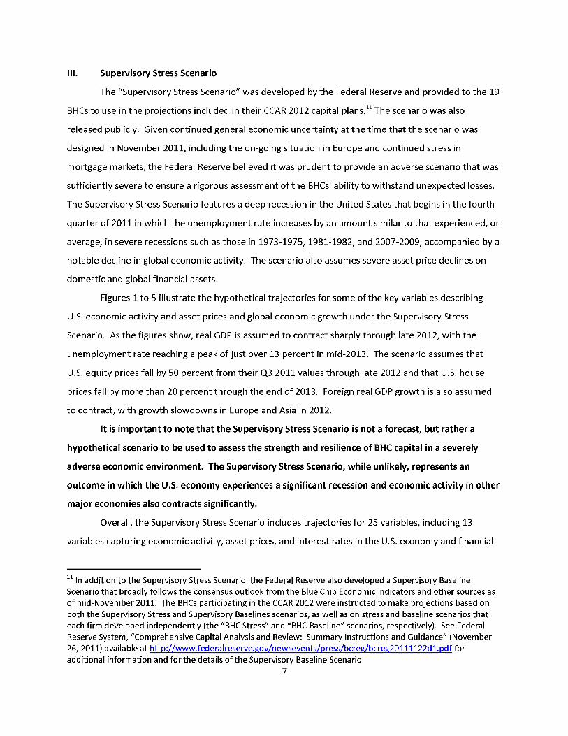
III. Supervisory Stress Scenario

The "Supervisory Stress Scenario" was developed by the Federal Reserve and provided to the 19

BHCs to use in the projections included in their CCAR 2012 capital plans.

[footnote] 11 In addition to the Supervisory Stress Scenario, the Federal Reserve also developed a Supervisory Baseline Scenario that broadly follows the consensus outlook from the Blue Chip Economic Indicators and other sources as of mid-November 2011. The BHCs participating in the CCAR 2012 were instructed to make projections based on both the Supervisory Stress and Supervisory Baselines scenarios, as well as on stress and baseline scenarios that each firm developed independently (the "BHC Stress" and "BHC Baseline" scenarios, respectively). See Federal Reserve System, "Comprehensive Capital Analysis and Review: Summary Instructions and Guidance" (November 26, 2011) available at http://www.federalreserve.gov/newsevents/press/bcreg/bcreg20111122d1.pdf for additional information and for the details of the Supervisory Baseline Scenario. [end of footnote 11.]

The scenario was also

released publicly. Given continued general economic uncertainty at the time that the scenario was

designed in November 2011, including the on-going situation in Europe and continued stress in

mortgage markets, the Federal Reserve believed it was prudent to provide an adverse scenario that was

sufficiently severe to ensure a rigorous assessment of the BHCs' ability to withstand unexpected losses.

The Supervisory Stress Scenario features a deep recession in the United States that begins in the fourth

quarter of 2011 in which the unemployment rate increases by an amount similar to that experienced, on

average, in severe recessions such as those in 1973-1975, 1981-1982, and 2007-2009, accompanied by a

notable decline in global economic activity. The scenario also assumes severe asset price declines on

domestic and global financial assets.

Figures 1 to 5 illustrate the hypothetical trajectories for some of the key variables describing

U.S. economic activity and asset prices and global economic growth under the Supervisory Stress

Scenario. As the figures show, real GDP is assumed to contract sharply through late 2012, with the

unemployment rate reaching a peak of just over 13 percent in mid-2013. The scenario assumes that

U.S. equity prices fall by 50 percent from their Q3 2011 values through late 2012 and that U.S. house

prices fall by more than 20 percent through the end of 2013. Foreign real GDP growth is also assumed

to contract, with growth slowdowns in Europe and Asia in 2012.

It is important to note that the Supervisory Stress Scenario is not a forecast, but rather a

hypothetical scenario to be used to assess the strength and resilience of BHC capital in a severely

adverse economic environment. The Supervisory Stress Scenario, while unlikely, represents an

outcome in which the U.S. economy experiences a significant recession and economic activity in other

major economies also contracts significantly.

Overall, the Supervisory Stress Scenario includes trajectories for 25 variables, including 13

variables capturing economic activity, asset prices, and interest rates in the U.S. economy and financial

markets, and three variables (real GDP growth, inflation, and the U.S./foreign currency exchange rate) in

each of four counties/country blocks (the euro area, the United Kingdom, developing Asia, and Japan).

The scenario starts in the fourth quarter of 2011 and extends through the fourth quarter of 2014, which

permits calculation of the ALLL at the end of 2013. Appendix A contains a description of the variables

included in the Supervisory Stress Scenario, as well as the trajectories for those variables between Q4

2011 and Q4 2014.

Figure 1: Real GDP Growth Rate in the Supervisory Stress Scenario (Q/Q seasonally adjusted growth rates annualized, Percent)

Q1 2009 -Q4 2014

[For the accessible version of this figure, please see the accompanying HTML.]

Figure 2: Unemployment Rate in the Supervisory Stress Scenario (Percent)

Q1 2009-Q4 2014

[For the accessible version of this figure, please see the accompanying HTML.]

Figure 3: Dow Jones Total Stock Market Index, End of Quarter Q1 2009 - Q4 2014

[For the accessible version of this figure, please see the accompanying HTML.]

Figure 4: National House Price Index in the Supervisory Stress Scenario Q1 2009 - Q4 2014

[For the accessible version of this figure, please see the accompanying HTML.]

Figure 5: Real GDP Growth in Four Country/Country Block Areas in the Supervisory Stress Scenario

(Q/Q seasonally adjusted growth rates annualized, percent) Q1 2009 -Q4 2014

[For the accessible version of this figure, please see the accompanying HTML.]

IV. Federal Reserve Stress Scenario Projections

This section describes the approach used to generate the Federal Reserve's stress scenario

projections of losses, revenue, expenses, and capital positions for the 19 BHCs participating in CCAR

2012. These projections were made by Federal Reserve analysts using input data provided by the 19

BHCs and models developed or selected by Federal Reserve staff. The projections are based on the

Supervisory Stress Scenario developed by the Federal Reserve. This scenario is not a forecast, but rather

a hypothetical scenario developed to assess the strength and resilience of BHC capital in a particularly

adverse economic and financial market environment. As such, the Federal Reserve's stress scenario

projections for the 19 BHCs should not be interpreted as expected or likely outcomes for these firms,

but as possible results under specific, hypothetical, severely adverse conditions. Other types of stressful

scenarios would be expected to generate different sets of stress results. Further, because the

projections are based on a set of standardized models applied to all 19 BHCs, they will differ from

projections that the individual BHCs will make of their own performance under the same set of

hypothetical adverse conditions.

The output of the stress scenario projections are estimates of regulatory capital ratios for each

of the 19 BHCs over the nine-quarter forward-looking stress scenario horizon. The capital ratios include

the ratio of tier 1 capital to risk-weighted assets (the tier 1 ratio), the ratio of total regulatory capital to

risk-weighted assets (the total capital ratio), the ratio of tier 1 capital to average assets (the tier 1

leverage ratio),

[footnote] 12

Tier 1 capital, as defined in the Board's Risk-Based Capital Adequacy Guidelines, is composed of common and non-common equity elements, some of which are subject to limits on their inclusion in tier 1 capital. See 12 CFR part 225, Appendix A, § II.A.1. These elements include common stockholders' equity, qualifying perpetual preferred stock, certain minority interests, and trust preferred securities. Certain intangible assets, including goodwill and deferred tax assets, are deducted from tier 1 capital or are included subject to limits. See 12 CFR part 225, Appendix A, § II.B. Total capital consists of tier 1 capital plus certain subordinated debt instruments and the allowance for loan and lease losses, subject to certain limits. [end of footnote 12.]

and the ratio of the common equity component of tier 1 capital to risk-weighted assets

(the tier 1 common ratio). As noted, the stress scenario projections are made under the Supervisory

Stress Scenario, which includes quarterly trajectories for U.S. and international macroeconomic and

financial market variables. The last historical period in the analysis is Q3 2011 and capital ratios are

projected quarterly through Q4 2013. That is, the stress scenario horizon is the nine-quarter period

from Q4 2011 to Q4 2013.

The Federal Reserve's projections assume the planned capital actions included in each BHC's

capital plan under its own baseline scenario ("BHC Baseline Scenario").

[footnote] 13 These capital actions include both actions that affect common equity and actions that affect non-common equity capital elements, such as certain forms of preferred stock. [end of footnote 13.]

As a result, the Federal

Reserve's projections do not incorporate any changes in dividends, share repurchases, or issuances that

BHCs might undertake in reaction to stressed financial conditions. This conservative assumption is part

of a supervisory exercise and in practice the Federal Reserve expects BHCs to follow the capital

conservation policies that are part of their capital plans. For example, the capital policies of some of the

BHCs contain triggers or guidelines for reducing capital distributions such as dividends and share

repurchases in conditions where profitability is reduced and/or capital ratios fall below certain internal

target levels.

[footntoe] 14 See http://www.federalreserve.gov/newsevents/press/bcreg/bcreg20111122d1.pdf for a more detailed description of the Federal Reserve's assessment of planned capital actions in CCAR 2012. [end of footnote 14.]

The projected stressed capital ratios evaluated in CCAR 2012 reflect the combined impact of the

stress scenario and each BHC's planned capital distributions. To illustrate the impact of the stress

scenario alone, the Federal Reserve also calculated stressed capital ratios excluding capital actions

planned for after Q1 2012.

[footnote] 15 The ratios assume planned capital actions through Q1 2012, but no material capital issuances from March 16 through March 31, 2012. [end of footntoe 15.]

The resulting stressed capital ratios could be higher or lower than those

including all the planned capital actions, depending on when the two minimum values occur (they could

come in different points of the stress scenario horizon), potential differences in risk-weighted assets at

those points, and whether those planned actions represent net additions or reductions in regulatory

capital.

As a policy matter, the Federal Reserve's stress scenario projections embed a number of

conservative assumptions that, on net, are likely to further reduce the projected levels of regulatory

capital under the Supervisory Stress Scenario. These assumptions often involve situations in which there

is considerable uncertainty about the impact of the hypothetical adverse economic and financial market

conditions in the Supervisory Stress Scenario on particular aspects of the BHCs' performance. In some

cases, this uncertainty arises because historical data provide limited guidance about the losses or

revenue being projected, while in other cases, the current state of modeling technique and practice

results in limitations on the precision of independent supervisory models. In these cases, as a policy

matter, the Federal Reserve opted to incorporate simplifying, conservative modeling assumptions that

tend to generate higher projections of loss and lower projections of revenue.

The Federal Reserve's stress scenario projections address the on-going situation in Europe

through several channels. The Supervisory Stress Scenario incorporates a hypothetical sharp downturn

in economic activity in the Euro area, and the global financial market shock applied to trading, private

equity, and derivatives positions of the largest BHCs includes very significant widening of credit default

swap spreads for both European sovereigns and financial institutions and sharp increases in spreads

across the yield curve for European sovereign bonds. These stresses affect many aspects of the stress

scenario projections, including projected losses on international lending portfolios, on sovereign and

financial institution bonds held in the BHCs' investment portfolios, and on trading, private equity, and

derivatives positions.

IV.A Analytical Framework

This section describes the analytical framework underlying the Federal Reserve's stress scenario

projections. The basic approach is to project the impact of the adverse economic environment in the

Supervisory Stress Scenario on the quarterly net income of each BHC, and then to carry forward the

impact of net income and each BHC's planned capital actions on regulatory capital measures in every

quarter of the stress scenario horizon. This approach provides a perspective on the capital of the BHCs

that is consistent with U.S. accounting (GAAP) and regulatory capital rules and on the primary drivers of

the projected changes in capital over time, through earnings and capital actions.

To generate projections of net income for the 19 BHCs, projections are made for revenue,

expenses, and various types of losses and provisions that flow into pre-tax net income, including losses

on loans and investment securities, losses generated by operational risk events, expenses related to

demands by mortgage investors to repurchase loans deemed to have breached representations and

warranties or related to litigation ("mortgage repurchase/put-back losses")

[footnote] 16 These estimates are conditional on the hypothetical adverse macroeconomic scenario and on conservative assumptions. They are not a supervisory estimate of the current legal liability that BHCs might actually face. [end of footnote 16.]

changes in the income

from mortgage servicing rights (MSRs), and, for BHCs with large trading operations, losses on trading

and counterparty positions under a severe shock to global financial market rates and prices. Projected

net income in turn flows into a calculation of regulatory capital measures, taking account of taxes and

deductions that limit the recognition of certain intangible assets and impose other restrictions, as

specified in current U.S. regulatory capital guidelines.

[footnote] 17 See generally, 12 CFR part 225, Appendix A. [end of footnote 17.]

As noted above, the projected capital measures

also incorporate each BHC's planned capital actions under its own baseline scenario. The Box on page

14 illustrates how the various elements of these calculations lead to projected net income and then to

projected changes in regulatory capital.

Since the stress scenario projections are intended to produce estimates of regulatory capital

ratios, the loss and revenue projections follow U.S. GAAP and regulatory guidelines. This approach

captures differences in the way that income and losses are recognized based on where assets are held

on the BHCs' balance sheets, generating sometimes greatly different loss projections for similar or

identical assets held in different portfolios. Specifically, losses on loans held in accrual portfolios are

calculated as credit losses due to failure to pay obligations (cash flow losses resulting in net charge-offs),

rather than discounts related to mark-to-market values. In some cases, BHCs may have loans that are

being held for sale or that are subject to purchase accounting adjustments. In these cases, loss

projections anticipate the change in value of the underlying asset, apply the appropriate accounting

treatment, and determine the incremental loss. Separate loss projections are made for different

categories of loans based on the type of obligor (e.g., consumer or commercial and industrial), collateral

(e.g., residential real estate, commercial real estate), or loan structure (e.g., revolving credit lines).

These categories generally follow the major regulatory report classifications, though some loss

projections are made for more granular loan categories than those included on BHC regulatory reports.

[footnote] 18 See Consolidated Financial Statements for Bank Holding Companies (FR Y-9C). [end of footnote 18.]

Losses on securities held in the available for sale (AFS) or held to maturity (HTM) accounts are

projected other-than-temporary impairments (OTTI) for these positions plus estimates of realized gains

or losses on certain securities sales. Following U.S. GAAP, OTTI projections incorporate other-than-

temporary differences between book value and fair value due to credit impairment, but not differences

reflecting changes in liquidity or market conditions. As with the accrual loan portfolio, loss projections

are made for different categories of securities based on obligor, collateral or underlying cash flow, and

security structure. These categories include various types of securitized obligations (e.g., commercial

and residential mortgage-backed securities), corporate bonds, municipal bonds, and sovereign bonds.

Estimates of realized gains or losses on securities sales are derived from information provided by the

BHCs on the sale of securities under contracts in place prior to September 30, 2011.

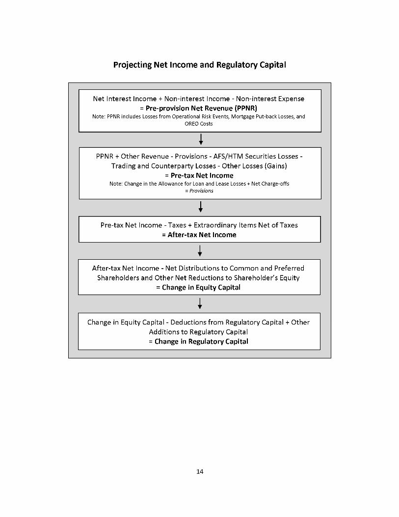
Projecting Net Income and Regulatory Capital [flow chart]

Net Interest Income + Non-interest Income - Non-interest Expense = Pre-provision Net Revenue (PPNR)

Note: PPNR includes Losses from Operational Risk Events, Mortgage Put-back Losses, and OREO Costs

[then:]

PPNR + Other Revenue - Provisions - AFS/HTM Securities Losses -Trading and Counterparty Losses - Other Losses (Gains)

= Pre-tax Net Income Note: Change in the Allowance for Loan and Lease Losses + Net Charge-offs

= Provisions [then:]

Pre-tax Net Income - Taxes + Extraordinary Items Net of Taxes = After-tax Net Income

[then:]

After-tax Net Income - Net Distributions to Common and Preferred Shareholders and Other Net Reductions to Shareholder's Equity

= Change in Equity Capital [then:]

Change in Equity Capital - Deductions from Regulatory Capital + Other Additions to Regulatory Capital = Change in Regulatory Capital.

For the six BHCs with large trading operations, losses on trading, derivatives, and private equity

positions are projected assuming an instantaneous re-pricing under a "global financial market shock."

The global financial market shock was developed by the Federal Reserve and reflects a period of

significant stress across a very broad range of markets and asset classes similar to that which occurred

during the second half of 2008, as well as additional stresses related to the on-going situation in Europe.

The global financial market shock is distinct and separate from the Supervisory Stress Scenario in that it

presumes a set of severe, instantaneous changes in market rates, prices, and volatilities that are in

effect layered over the financial market variables contained in the Supervisory Stress Scenario. Losses

related to the global financial market shock are assumed to occur in the first quarter of the stress

scenario projections (Q4 2011). These losses include mark-to-market and incremental default-related

losses on each of the six BHCs' trading and private equity positions, as well as changes in credit valuation

adjustments (CVA) for counterparty exposures. It is important to capture the impact of counterparty

credit risk, since projected mark-to-market losses on the trading account can be reduced if trading

positions are hedged, but the effectiveness of these hedges depends on counterparty performance on

the obligations. This impact is captured through the stress applied to counterparty credit exposures.

Pre-provision net revenue (PPNR) is calculated as projected net interest income plus non-

interest income minus non-interest expense. Consistent with U.S. GAAP, PPNR projections incorporate

projected losses related to operational risk events such as fraud, computer system or other operating

disruptions, or employee lawsuits; repurchase and litigation expenses related to residential mortgages;

projected changes in income from mortgage servicing rights; and expenses related to the disposition of

foreclosed properties (other real estate owned (OREO) expenses).

Projected net income incorporates provisions into the allowance for loan and lease losses

(ALLL). Provisions are determined so that the ALLL is at an appropriate level at the end of each quarter

given projected loan losses in that quarter, where the appropriate level of the ALLL is a function of

projected future loan losses. This calculation could lead either to a drawdown of the ALLL (an ALLL

release, increasing net income) or the need to build the ALLL (an additional provision, decreasing net

income) during the quarter. Total provisions into the ALLL are calculated as projected loan losses for the

quarter plus or minus the amount needed for the ALLL to be at an appropriate level at the end of the

quarter.

The Federal Reserve's forward-looking projections of income and losses may include the effects

of planned mergers or acquisitions or the initiation of new business lines or activities that were included

in the BHCs' capital plans and are subject to prior approval or notice by the Federal Reserve or other

supervisors. The inclusion of the effects of such planned actions does not, and is not intended to,

express a view on the merits of such proposals and is not an approval or non-objection to them.

The final projection of pre-tax net income is the projection of PPNR minus provisions minus

projected losses on securities and losses from the global financial market shock (for the six BHCs with

large trading operations) minus losses on loans held for sale and measured under the fair value option.

Net income projections also incorporate one-time revenues and expenses and goodwill impairment

charges, as projected by the BHCs in their capital plans. After-tax net income is calculated by applying a

consistent tax rate to pre-tax net income for all BHCs. Along with each BHC's planned capital actions

(dividend payments, repurchases or redemptions, and issuance of common equity or other capital

instruments), after-tax net income is the primary driver of projected changes in equity capital, which in

turn drive projected changes in the regulatory capital measures that are the final output of the Federal

Reserve's stress scenario projections. Capital ratios are calculated using average total assets and risk-

weighted assets that are based on projections made by the BHCs as part of their CCAR 2012 capital plan

submissions under the Supervisory Stress Scenario.

IV.B Modeling Design and Implementation

The Federal Reserve's stress scenario projections are based on input data provided by the 19

BHCs participating in CCAR 2012 and on models developed or selected by Federal Reserve staff and

reviewed by an independent group of Federal Reserve economists and analysts. The models are

intended to capture the impact of the macroeconomic and financial market factors included in the

Supervisory Stress Scenario and characteristics of the BHCs' loans and securities portfolios; trading,

private equity, and derivatives positions; business activities; and other factors affecting losses, revenue,

and expenses. This section describes the input data provided by the BHCs and the approach the Federal

Reserve took in designing and implementing these models.

BHC Input Data

The 19 BHCs participating in CCAR 2012 were required to submit extensive data to the Federal

Reserve on a series of regulatory reports.

[footnote] 19 These report forms are the FR Y-14Q and FR Y-14A reports, which can be found at http://www.federalreserve.gov/reportforms/formsreview/FRY14Q 20111216 f.pdf and http://www.federalreserve.gov/reportforms/formsreview/FRY14A 20120118 f.pdf. [end of footnote 19.]

The reports capture information on the BHCs' loan and

securities portfolios as of September 30, 2011, including borrower characteristics, collateral

characteristics, characteristics of the loans or credit facilities, amounts outstanding and yet to be drawn

down (for credit lines), and payment history and current status. In some cases (primarily retail credit

portfolios), aggregated information is reported based on segments of the loan portfolios (e.g., segments

defined by loan-to-value (LTV) ratio, geographic location, and borrower credit score), while in other

cases, information is collected on individual loans or credit facilities. For securities held in the AFS and

HTM portfolios, information is collected at the individual security (CUSIP) level, including the amortized

cost, market value, and any OTTI taken on the security to date.

Additional reports collect information on trading and derivatives positions, private equity

holdings, and certain other assets subject to fair value accounting held by BHCs with large trading

operations. These reports collect BHC-estimated sensitivities of these positions to the set of risk factors

specified by the Federal Reserve, including changes in a wide range of U.S. and global financial market

rates and asset prices, and volatilities and correlations of those rates and prices. The specific risk factors

are those judged to be most relevant to the positions held by the BHCs. The reports also collect

information on the estimated sensitivity of the BHCs' counterparty-related profit or loss to these risk

factors, both for segments of the portfolio and for individual large counterparties. These data are used

in projecting losses related to the global financial market shock, including losses related to derivatives

and other counterparty exposures. These data were collected for positions in the trading and private

equity portfolios held by the BHCs as of market close on November 17, 2011.

[footnote]20 The BHCs were informed of the portfolio date for the global market risk analysis when the CCAR 2012 instructions were released on November 22, 2011. [end of footnote 20.]

A final set of reports collects information on historical and projected revenues and operating

and other non-credit-related expenses for each BHC. This information includes data on net interest

income, non-interest income, and expenses by business line, as well as a series of metrics (balances,

volumes of trades and transactions, assets under management, fee schedules, compensation expenses)

related to a range of business activities conducted by the BHCs. Data are also collected on the BHCs'

historical losses related to operational risk events. These data, both historical and the BHCs' projections

of these amounts over the stress scenario horizon, were used in developing the Federal Reserve's

projections of PPNR for the 19 BHCs. Finally, the reports collect information on the BHCs' projections of

risk-weighted assets, balance sheet composition, and capital over the stress scenario horizon.

All 19 BHCs participating in CCAR 2012 were required to submit these regulatory reports to the

Federal Reserve by either late December (for forms containing detailed loan and securities portfolio

information) or early January (for forms containing BHC-derived estimates).

[footnote] 21 Specifically, the BHCs were required to submit the FR Y-14Q reports (containing, among other items, detailed loan and securities portfolio information) by December 15, 2011. The BHCs were required to submit the FR Y-14A reports (containing, among other items, the BHC-derived estimates) by January 9, 2012. [end of footnote 21.]

BHCs were required to

submit detailed loan and securities portfolio information for all material portfolios, where "material"

was defined as those portfolios exceeding either 5 percent of tier 1 capital or $5 billion and the portfolio

categories were defined on the regulatory reports. For portfolios falling below these thresholds, the

BHCs had the option to submit or not submit the detailed data. Portfolios for which the Federal Reserve

did not receive detailed data were assigned a loss rate equal to a high percentile of the loss rates

projected for BHCs that did submit data for that category of loan or security. For instances where

certain data elements were reported as missing values, these missing data were filled in with

conservative values (e.g., high LTV values or low credit scores) based on the remainder of the portfolio.

The stress scenario projections may include the effects of planned mergers or acquisitions or the

initiation of new business lines, as reported by BHCs in their CCAR 2012 capital plans. BHCs with

significant planned mergers or acquisitions provided available information on the characteristics of the

institutions or portfolios to be acquired. As noted above, the inclusion of the effects of such planned

actions does not and is not intended to express a view on the merits of such proposals and is not an

approval or non-objection to them.

Loss, Revenue, and Expense Models

The data collected from the BHCs, along with the variables defining the Supervisory Stress

Scenario, are inputs into a series of models used to project losses, revenues, and expenses for each BHC

over the stress scenario horizon. In most cases, these models were either developed by Federal Reserve

analysts and economists or are vendor-developed models used by Federal Reserve staff. In some cases,

however, the stress scenario projections of certain types of losses or revenue made by the Federal

Reserve rely on sensitivities generated by the BHCs using their internal risk measurement models or on

modeled estimates provided by the BHCs, along with supporting documentation, and assessed and

adjusted by Federal Reserve analysts. These are cases in which independent supervisory models are

either not yet sufficiently robust to generate reliable estimates or are technically and logistically

extremely difficult to implement.

[footnote] 22 The primary examples are models designed to capture the impact of changes to global financial market rates and prices on trading, private equity, and derivatives positions, where developing fully independent revaluation models that can capture the range of complex instruments and positions held by the BHCs is an extremely difficult undertaking, and models that can capture the BHC-specific factors determining the various elements of PPNR. [end of footnote 22.]

In general, the models were developed using pooled historical data from many financial

institutions, either supervisory data collected by the Federal Reserve or data purchased from industry

data aggregators. The models are thus "industry models" in the sense that the estimated parameters

reflect the typical or industry-average response to variation in the macroeconomic and financial market

variables and portfolio-specific and instrument-specific characteristics, rather than being tailored to the

way that each individual BHC's losses, revenues, or expenses might respond to these factors. This

approach reflects not only the difficulty of estimating separate, statistically robust models for each of

the 19 BHCs, but also the desire not to assume that historical BHC-specific results will prevail in the

future when those results cannot be explained by consistently observable variables incorporated into a

robust statistical model. Thus, BHC-specific factors are incorporated through the detailed portfolio and

business activity data that are inputs to the models, but the reaction functions to these variables and to

the macroeconomic and financial market factors defined in the Supervisory Stress Scenario are the same

for all BHCs. This means that the stress scenario projections made by the Federal Reserve will not

necessarily match or mirror similar projections made by individual BHCs, which will incorporate diverse

approaches to capturing the impact of portfolio characteristics and economic factors.

The models developed internally by the Federal Reserve draw on academic literature and

industry practice in modeling the impact of borrower, instrument, and collateral characteristics and

macroeconomic factors on losses, revenue, and expenses. The approaches build on work done by the

Federal Reserve in the SCAP and the 2011 CCAR, but in many cases represent significant refinement and

advancement of that work, reflecting advances in modeling technique, richer and more detailed data

over which to estimate the models, and longer histories of performance in both adverse and more

benign economic settings. The models were reviewed by an independent model review team composed

of economists and analysts from across the Federal Reserve System, with a focus on the design and

estimation of the models. In addition, Federal Reserve analysts developed industry-wide loss and PPNR

projections capturing the potential loss and revenue-generating rates of the banking industry as a whole

in a stressed macroeconomic environment, for use as reference points in assessing model outputs

across the 19 BHCs.

The models used in the stress scenario projections are described in greater detail in Appendix B.

Appendix A

Supervisory Stress Scenario

This Appendix provides a description of the Supervisory Stress Scenario provided by the Federal Reserve.

It is important to note that the Supervisory Stress Scenario is not a forecast but rather a

hypothetical scenario to be used to assess the strength and resilience of BHC capital in a severely

adverse economic environment. The Supervisory Stress Scenario, while unlikely, represents an

outcome in which the U.S. economy experiences a significant recession and economic activity in other

major economies also contracts significantly.

The scenario starts in the fourth quarter of 2011 and extends through the fourth quarter of

2014, which permits the calculation of loan-loss reserves at the end of 2013. The scenario is defined

over 25 variables. For the domestic U.S. variables, the scenario includes:

• Five measures of economic activity and prices: Real and nominal Gross Domestic Product (GDP), the

unemployment rate of the civilian non-institutional population aged 16 and over, nominal

disposable personal income, and the Consumer Price Index (CPI);

• Four aggregate measures of asset prices or financial conditions: The CoreLogic National House Price

Index, the National Council for Real Estate Investment Fiduciaries Commercial Real Estate Price

Index, the Dow Jones Total Stock Market Index, and the Chicago Board Options Exchange Market

Volatility Index; and,

• Four measures of interest rates: the rate on the three-month Treasury bill, the yield on the 10-year

Treasury bond, the yield on a 10-year BBB corporate security, and the interest rate associated with a

conforming, conventional, fixed-rate, 30-year mortgage.

For the international variables, the scenario includes three variables in four countries/country blocks.

• The three variables for each country/country block are the percent change in real GDP, the percent

change in the Consumer Price Index or local equivalent, and the U.S./foreign currency exchange

rate.

• The four countries/country blocks included are the euro area, the United Kingdom, developing Asia,

and Japan. The euro area is defined as the 17 European Union member states that have adopted

the euro as their common currency and developing Asia is defined as the aggregate of China, India,

Hong Kong, and Taiwan.

The preceding discussion describes the broad contours of the Supervisory Stress Scenario over

the period from 2012 to 2014. The specific values for all the variables included in the scenario are

shown on the following pages.

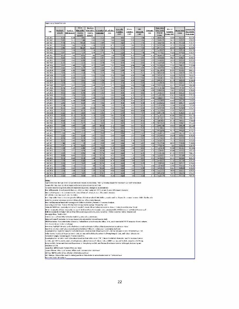
Supervisory Stress Scenario

OBS Real GDP growth Nominal

GDP growth

Real disposable

income growth

Nominal disposable

income growth

Unemploy ment rate CPI inflation rate 3-month Treasury

yield

10-year Treasury

yield

BBB corporate

yield

Mortgage rate

Dow Jones Total Stock

Market Index

Market Volatility

Index (VIX)

House Price index Commercial Real Estate Price Index

Q1 2001 -1.31 1.40 3.05 5.96 4.23 3.88 4.82 5.30 7.44 7.24 10,645.85 32.84 113.46 130.98

Q2 2001 2.65 5.47 -1.08 0.82 4.41 2.86 3.66 5.50 7.49 7.37 11,407.15 34.72 115.20 130.12

Q3 2001 -1.10 0.15 10.58 10.66 4.81 1.08 3.19 5.26 7.26 7.19 9,562.95 43.74 117.58 129.20

Q4 2001 1.41 2.66 -4.59 -4.38 5.53 -0.25 1.91 5.06 7.19 7.00 10,707.68 35.31 119.99 127.36 Q1 2002 3.46 4.93 11.23 12.25 5.70 1.25 1.72 5.39 7.58 7.20 10,775.74 26.09 122.44 129.05

Q2 2002 2.14 3.99 2.21 5.44 5.84 3.20 1.72 5.35 7.61 7.03 9,384.03 28.42 125.74 129.24

Q3 2002 2.04 3.82 -1.37 0.64 5.72 2.15 1.64 4.55 7.28 6.48 7,773.63 45.08 129.10 130.49

Q4 2002 0.14 2.46 0.95 2.86 5.84 2.40 1.34 4.29 7.04 6.25 8,343.19 42.64 131.56 131.77 Q1 2003 1.68 4.55 1.48 4.43 5.87 4.13 1.16 4.16 6.47 5.99 8,051.86 34.69 134.59 134.63

Q2 2003 3.43 4.64 6.19 6.50 6.15 -0.59 1.04 3.80 5.65 5.65 9,342.42 29.13 137.48 135.93

Q3 2003 6.75 9.14 5.71 8.47 6.10 2.99 0.93 4.40 6.02 6.18 9,649.68 22.72 141.68 137.10

Q4 2003 3.67 5.80 2.32 4.22 5.81 1.57 0.92 4.44 5.84 6.09 10,799.63 21.07 146.32 139.04 Q1 2004 2.66 6.28 1.79 5.19 5.68 3.43 0.92 4.14 5.45 5.75 11,039.42 21.58 152.67 141.22

Q2 2004 2.60 6.11 4.01 7.11 5.58 3.16 1.08 4.75 6.08 6.31 11,138.91 19.96 159.10 143.52

Q3 2004 3.01 6.03 2.70 5.25 5.43 2.58 1.49 4.45 5.77 6.06 10,895.48 19.34 164.33 146.53

Q4 2004 3.31 6.43 5.71 9.15 5.38 4.39 2.01 4.30 5.44 5.89 11,971.14 16.58 170.25 147.61

Q1 2005 4.19 8.09 -4.79 -2.51 5.27 2.05 2.54 4.39 5.43 5.91 11,638.27 14.65 180.11 148.12 Q2 2005 1.79 4.55 2.85 5.40 5.10 2.68 2.86 4.24 5.46 5.87 11,876.74 17.74 186.45 174.64

Q3 2005 3.21 7.52 2.41 7.10 4.95 6.24 3.36 4.29 5.48 5.92 12,289.26 14.17 192.51 175.76

Q4 2005 2.07 5.54 2.21 5.84 4.94 3.72 3.83 4.60 5.88 6.40 12,517.69 16.47 197.07 186.38

Q1 2006 5.15 8.31 7.71 9.52 4.71 2.13 4.39 4.67 5.97 6.42 13,155.44 14.56 201.82 195.50 Q2 2006 1.63 5.24 3.60 6.70 4.64 3.68 4.71 5.15 6.48 6.80 12,849.29 23.81 199.55 198.00

Q3 2006 0.05 3.11 1.94 4.90 4.63 3.83 4.91 4.96 6.43 6.77 13,345.97 18.64 198.29 199.43

Q4 2006 2.75 4.59 5.35 5.26 4.44 -1.69 4.90 4.70 6.12 6.43 14,257.55 12.67 198.93 215.76

Q1 2007 0.54 5.23 1.82 5.83 4.49 3.92 4.98 4.76 6.11 6.40 14,409.27 19.63 196.43 222.91

Q2 2007 3.65 6.50 0.60 4.08 4.47 4.76 4.74 4.92 6.30 6.55 15,210.65 18.89 191.35 229.81 Q3 2007 2.96 4.34 1.59 3.85 4.65 2.44 4.31 4.84 6.54 6.75 15,362.02 30.83 185.77 221.46

Q4 2007 1.70 3.64 2.23 6.52 4.80 4.92 3.40 4.41 6.37 6.41 14,819.58 31.09 179.99 222.88

Q1 2008 -1.76 0.58 5.90 10.00 4.95 4.51 2.07 3.87 6.54 6.04 13,332.01 32.24 173.04 223.71

Q2 2008 1.32 4.03 8.22 13.11 5.31 5.31 1.62 4.09 6.84 6.26 13,073.54 31.01 165.31 217.79 Q3 2008 -3.66 -0.57 -8.82 -4.86 6.03 6.46 1.49 4.05 7.19 6.50 11,875.41 46.72 158.25 217.11

Q4 2008 -8.89 -8.43 -0.23 -5.79 6.91 -9.07 0.30 3.72 9.39 6.03 9,087.17 80.86 149.51 189.54

Q1 2009 -6.67 -5.23 -3.81 -5.42 8.22 -2.50 0.21 3.23 8.96 5.18 8,113.14 56.65 142.77 186.93

Q2 2009 -0.69 -1.14 0.25 2.15 9.29 1.97 0.17 3.65 8.15 5.14 9,424.92 42.28 143.51 154.64 Q3 2009 1.70 1.93 -5.42 -2.57 9.69 3.67 0.16 3.81 6.76 5.28 10,911.69 31.30 144.81 157.50

Q4 2009 3.80 4.88 -0.58 2.18 10.01 2.72 0.06 3.69 6.13 5.03 11,497.41 30.69 145.34 152.24

Q1 2010 3.94 5.52 4.86 6.81 9.70 1.28 0.11 3.87 5.78 5.11 12,160.97 27.31 146.66 157.50

Q2 2010 3.79 5.43 5.57 5.91 9.66 -0.51 0.15 3.62 5.55 5.02 10,750.01 45.79 146.10 171.27

Q3 2010 2.51 3.86 2.27 3.27 9.59 1.42 0.16 2.90 5.07 4.54 11,947.14 32.86 141.78 160.45 Q4 2010 2.35 4.16 1.50 3.47 9.63 2.68 0.14 2.97 5.04 4.50 13,290.03 23.54 139.61 178.95

Q1 2011 0.36 3.09 1.24 5.19 8.93 5.25 0.13 3.53 5.40 4.95 14,036.43 29.40 137.93 177.17

Q2 2011 1.34 3.96 0.59 3.91 9.06 4.02 0.05 3.28 5.15 4.76 13,968.11 22.73 137.56 173.82

Q3 2011 2.46 5.04 -1.73 0.59 9.09 3.09 0.02 2.48 4.87 4.40 11,771.86 48.00 136.86 174.08 Q4 2011 -4.84 -1.70 -6.02 -3.37 9.68 2.21 0.10 2.07 5.65 4.65 9,501.48 75.86 135.13 168.40

Q1 2012 -7.98 -5.39 -6.81 -5.30 10.58 1.78 0.10 1.94 6.83 5.12 7,576.38 90.50 131.61 161.04

Q2 2012 -4.23 -2.54 -4.29 -3.46 11.40 1.02 0.10 1.76 6.81 5.16 7,089.87 80.00 127.50 153.42

Q3 2012 -3.51 -2.24 -3.16 -2.44 12.16 0.89 0.10 1.67 6.75 5.17 5,705.55 81.23 123.12 146.53 Q4 2012 0.00 0.09 -0.57 -0.36 12.76 0.35 0.10 1.76 6.45 5.08 5,668.34 69.82 119.08 139.36

Q1 2013 0.72 0.58 0.74 0.84 13.00 0.23 0.10 1.74 6.07 4.93 6,082.47 62.75 115.15 136.75

Q2 2013 2.21 2.01 1.66 1.74 13.05 0.21 0.10 1.84 5.83 4.82 6,384.32 57.76 111.92 135.20

Q3 2013 2.32 2.14 2.69 2.88 12.96 0.30 0.10 1.98 5.74 4.77 7,084.65 53.82 109.77 134.02

Q4 2013 3.45 3.26 2.27 2.48 12.76 0.32 0.10 1.98 5.51 4.66 7,618.89 49.84 108.48 134.36 Q1 2014 3.36 2.94 2.77 2.62 12.61 -0.03 0.10 1.97 5.28 4.54 8,014.71 45.87 108.08 134.45

Q2 2014 3.71 3.18 3.53 3.25 12.36 -0.16 0.10 1.88 4.94 4.38 9,925.73 34.96 108.40 135.91

Q3 2014 4.64 4.09 2.82 2.53 12.04 -0.17 0.10 1.86 4.72 4.26 10,874.38 24.22 109.24 139.53

Q4 2014 4.64 4.00 4.48 4.01 11.66 -0.34 0.10 1.89 4.58 4.17 12,005.11 17.51 110.29 143.35

Notes: Sources for data through 2011: Q3 (as released through 11/08/2010). 2011:Q3 international GDP data based on staff calculations. Values after that date equal assumptions for the supervisory stress scenario. Variables reported as growth rates are expressed as percent changes at an annual rate. Real GDP growth: Gross Domestic Product, billions of chain-weighted 2005 dollars, Bureau of Economic Analysis Nominal GDP growth: Gross Domestic Product, billions of dollars, Bureau of Economic Analysis CPI inflation rate: Bureau of Labor Statistics Real Disposable Personal Income growth: Billions of chain-weighted 2002 dollars, equals nominal disposable personal income divided by the price index for personal consumption expenditures, Bureau of Economic Analysis Nominal Disposable Personal Income growth: Billions of dollars, Bureau of Economic Analysis Unemployment Rate: Bureau of Labor Statistics (quarterly average of monthly data) 3-Month T-Bill Rate: Quarterly average of 3-month Treasury bill secondary market rate discount basis, Federal Reserve Board 10-yr Treasury Bond Rate: Quarterly average of yield on 10-yr U.S. Treasury bond, constructed for FRB/US model by Federal Reserve staff BBB Corporate Bond Rate: Yield on 10-yr BBB-rated corporate bond, constructed for FRB/US model by Federal Reserve staff Mortgage Rate: Freddie Mac Dow Jones Total Stock Market Index: End of quarter value, Dow Jones National House Price Index: CoreLogic (seasonally adjusted by Federal Reserve staff) CRE Price Index: Composite index created by Federal Reserve staff using the office, retail, and industrial NCREIF Transaction Based Indexes. VIX: Chicago Board Options Exchange

Euro Area Real GDP Growth: staff calculations based on Statistical Office of the European Communities via Haver Euro Area Inflation: staff calculations based on Statistical Office of the European Community via Haver Developing Asia Real GDP Growth: staff calculations based on Bank of Korea via Haver, Chinese National Bureau of Statistics via CEIC, Indian Central Statistical Organization via CEIC, Census and Statistics Department of Hong Kong via CEIC, and Taiwan Directorate-General of Budget, Accounting and Statistics via CEIC.

Developing Asia Inflation: staff calculations based on Bank of Korea via CEIC, Chinese Statistical Information and Consultancy Service via CEIC, and IMF Recent Economic Developments, Labour Bureau of India via CEIC and IMF, Census and Statistic Department of Hong Kong via CEIC, Census and Statistics Department of Hong Kong via CEIC, and Taiwan Directorate-General of Budget, Accounting and Statistics via CEIC.

Japan Real GDP Growth: Cabinet Office via Haver Japan Inflation: Ministry of Internal Affairs and Communications via Haver UK Real GDP Growth: Office of National Statistics via Haver

UK Inflation: Office of National Statistics (uses Retail Price Index to extend series back to 1960) via Haver Exchange Rates: Bloomberg

Supervisory Stress Scenario

OBS Euro Area Real GDP Growth

Euro Area Inflation

Euro Area Bilateral

Dollar Exchange

Rate ($/Euro)

Developing Asia Real

GDP Growth

Developing Asia

Inflation

Developing Asia

Bilateral Dollar

Exchange Rate

(F/USD, Index, Base = 2000 0 1 )

Japan Real GDP Growth

Japan Inflation

Japan Bilateral

Dollar Exchange

Rate (Yen/USD)

UK Real GDP Growth

UK Inflation

UK Bilateral Dollar

Exchange Rate

(USD/Pound)

Q1 2001 3.70 1.06 0.88 3.82 1.59 105.90 1.79 0.55 125.54 5.38 0.09 1.43

Q2 2001 0.32 4.03 0.85 5.69 1.98 105.99 -2.36 -2.00 124.73 1.68 3.02 1.41

Q3 2001 0.16 1.44 0.91 4.45 1.20 106.29 -4.63 -0.59 119.23 2.66 1.02 1.47

Q4 2001 0.50 1.69 0.89 6.50 -0.25 106.74 -1.75 -1.85 131.04 1.60 0.04 1.45

Q1 2002 0.91 2.97 0.87 7.16 0.32 107.20 1.19 -1.11 132.70 3.31 1.90 1.43

Q2 2002 2.01 2.01 0.99 8.73 0.65 104.67 3.24 0.08 119.85 2.60 0.88 1.52

Q3 2002 1.34 1.62 0.99 4.71 1.44 105.41 3.09 -0.44 121.74 3.17 1.34 1.56 Q4 2002 0.20 2.38 1.05 6.06 0.71 104.39 0.36 -0.59 118.75 2.75 1.92 1.61

Q1 2003 -0.11 3.24 1.09 6.63 3.14 105.40 -1.57 -0.04 118.07 2.73 1.58 1.59

Q2 2003 0.06 0.34 1.15 2.59 1.16 103.93 2.54 0.24 119.87 4.77 0.29 1.67

Q3 2003 2.03 2.17 1.16 12.51 -0.01 102.59 2.95 -0.64 111.43 4.07 1.70 1.67

Q4 2003 2.48 2.16 1.27 11.00 5.38 103.31 5.47 -0.72 107.13 4.79 1.65 1.79

Q1 2004 2.27 2.32 1.23 4.57 4.11 101.39 4.55 0.60 104.18 3.06 1.31 1.85

Q2 2004 2.12 2.34 1.22 5.98 3.92 102.73 -1.05 -0.36 109.43 1.40 0.98 1.82 Q3 2004 1.65 2.00 1.23 8.32 3.84 102.67 2.47 -0.04 110.20 0.53 1.02 1.82

Q4 2004 1.30 2.40 1.35 7.44 0.71 98.97 -1.79 1.75 102.68 1.92 2.36 1.92

Q1 2005 0.67 1.50 1.30 7.81 2.80 98.66 2.92 -0.91 107.22 1.27 2.55 1.89

Q2 2005 3.02 2.13 1.20 6.90 1.68 99.00 4.55 -1.19 110.91 3.19 1.85 1.79

Q3 2005 2.41 3.12 1.20 9.31 2.44 98.55 2.79 -1.36 113.29 3.38 2.68 1.75

Q4 2005 2.38 2.46 1.19 9.92 1.77 98.12 1.15 0.68 117.88 3.32 1.35 1.72

Q1 2006 3.86 1.62 1.22 11.60 2.37 96.84 0.01 1.31 117.48 3.08 1.90 1.75 Q2 2006 4.27 2.44 1.28 7.53 2.96 96.73 4.51 0.00 114.51 1.50 2.95 1.85

Q3 2006 2.67 1.99 1.27 8.36 1.77 96.32 1.30 0.40 117.99 0.90 3.21 1.89

Q 4 2 0 0 6 3.95 0.94 1.32 9.89 3.96 94.58 2.50 -0.40 119.02 2.72 2.60 1.96

Q1 2007 3.53 2.21 1.33 13.97 3.75 93.97 4.60 -0.24 117.56 4.23 2.70 1.96

Q2 2007 1.91 2.24 1.35 9.72 4.63 91.93 1.10 0.00 123.39 4.65 1.53 2.00

Q3 2007 2.42 2.07 1.43 8.50 7.22 90.62 -1.18 0.12 114.97 4.79 0.19 2.04

Q4 2007 1.51 4.87 1.47 9.25 6.17 89.38 2.50 2.26 111.71 2.56 3.92 2.00 Q1 2008 2.36 4.14 1.59 8.73 7.65 87.94 2.79 1.30 99.85 0.10 3.81 2.00

Q2 2008 -1.54 3.10 1.56 6.50 5.99 88.55 -4.66 1.69 106.17 -5.09 5.33 2.00

Q3 2008 -2.10 3.04 1.41 4.21 2.72 91.24 -5.38 3.28 105.94 -7.92 5.59 1.79

Q4 2008 -7.21 -1.26 1.39 -0.53 -1.27 91.95 -11.81 -2.34 90.79 -9.12 0.51 1.47

Q1 2009 -10.81 -1.07 1.33 5.33 -1.25 94.02 -19.91 -3.14 99.15 -6.32 0.33 1.43

Q2 2009 -0.85 -0.11 1.41 12.71 2.16 92.05 7.79 -1.74 96.42 -0.81 1.82 1.64

Q3 2009 1.77 0.96 1.47 12.11 4.46 91.12 -1.75 -1.83 89.49 0.93 3.29 1.61 Q4 2009 1.54 1.92 1.43 7.26 5.25 90.55 6.54 -1.36 93.08 2.94 3.08 1.61

Q1 2010 1.32 1.76 1.35 10.74 4.71 89.79 8.91 1.36 93.40 0.64 4.58 1.52

Q2 2010 3.69 1.68 1.23 7.10 3.09 90.89 -0.66 -1.20 88.49 4.20 2.57 1.49

Q 3 2 0 1 0 1.62 1.53 1.35 8.78 3.97 88.27 3.96 -2.68 83.53 2.47 1.96 1.56

Q 4 2 0 1 0 1.07 3.01 1.33 6.36 7.98 87.19 -2.41 1.32 81.67 -2.05 4.27 1.54

Q1 2011 3.10 3.59 1.41 9.05 6.18 86.44 -3.77 0.40 82.76 1.58 7.22 1.61

Q2 2011 0.65 2.75 1.45 7.54 4.75 85.25 -2.17 -0.80 80.64 0.41 3.68 1.61 Q3 2011 1.33 1.24 1.35 7.52 5.38 87.66 1.01 0.08 77.04 0.70 3.28 1.56

Q4 2011 -1.03 2.53 1.32 5.76 6.12 89.53 1.63 -0.76 77.20 -0.29 2.64 1.56

Q1 2012 -3.49 1.69 1.30 4.93 4.75 91.49 0.48 -1.53 77.94 -1.60 1.50 1.56

Q2 2012 -5.40 0.29 1.25 4.69 3.18 94.91 -1.29 -2.43 78.25 -2.93 0.26 1.55

Q3 2012 -6.91 -0.99 1.19 4.67 2.07 100.27 -3.94 -3.85 78.95 -4.25 -0.90 1.53

Q4 2012 -4.92 -0.92 1.18 6.86 1.22 98.96 -4.23 -3.44 79.14 -3.61 -0.70 1.54

Q1 2013 -2.64 -0.49 1.18 7.91 1.08 97.48 -3.51 -3.19 79.25 -2.41 -0.35 1.53 Q2 2013 -0.88 0.02 1.18 8.23 1.12 95.89 -2.66 -2.78 79.32 -1.19 0.12 1.53

Q3 2013 0.35 0.43 1.19 8.25 1.21 94.26 -1.77 -2.34 79.38 -0.10 0.57 1.53

Q4 2013 1.11 0.71 1.19 8.18 1.32 92.66 -0.92 -1.93 79.43 0.76 0.95 1.52

Q1 2014 1.50 0.87 1.20 8.15 1.44 91.15 -0.14 -1.56 79.51 1.39 1.25 1.52

Q2 2014 1.68 0.99 1.20 8.16 1.57 89.75 0.44 -1.25 79.58 1.83 1.49 1.52

Q3 2014 1.74 1.11 1.20 8.21 1.73 88.45 0.83 -0.99 79.63 2.12 1.69 1.52

Q4 2014 1.72 1.23 1.21 8.28 1.89 87.25 1.05 -0.76 79.62 2.30 1.84 1.52

Notes: Sources for data through 2011: Q3 (as released through 11/08/2010). 2011:Q3 international GDP data based on staff calculations. Values after that date equal assumptions for the supervisory stress scenario. Variables reported as growth rates are expressed as percent changes at an annual rate. Real GDP growth: Gross Domestic Product, billions of chain-weighted 2005 dollars, Bureau of Economic Analysis Nominal GDP growth: Gross Domestic Product, billions of dollars, Bureau of Economic Analysis CPI inflation rate: Bureau of Labor Statistics Real Disposable Personal Income growth: Billions of chain-weighted 2002 dollars, equals nominal disposable personal income divided by the price index for personal consumption expenditures, Bureau of Economic Analysis Nominal Disposable Personal Income growth: Billions of dollars, Bureau of Economic Analysis Unemployment Rate: Bureau of Labor Statistics (quarterly average of monthly data) 3-Month T-Bill Rate: Quarterly average of 3-month Treasury bill secondary market rate discount basis, Federal Reserve Board 10-yr Treasury Bond Rate: Quarterly average of yield on 10-yr U.S. Treasury bond, constructed for FRB/US model by Federal Reserve staff BBB Corporate Bond Rate: Yield on 10-yr BBB-rated corporate bond, constructed for FRB/US model by Federal Reserve staff Mortgage Rate: Freddie Mac Dow Jones Total Stock Market Index: End of quarter value, Dow Jones National House Price Index: CoreLogic (seasonally adjusted by Federal Reserve staff) CRE Price Index: Composite index created by Federal Reserve staff using the office, retail, and industrial NCREIF Transaction Based Indexes. VIX: Chicago Board Options Exchange

Euro Area Real GDP Growth: staff calculations based on Statistical Office of the European Communities via Haver Euro Area Inflation: staff calculations based on Statistical Office of the European Community via Haver Developing Asia Real GDP Growth: staff calculations based on Bank of Korea via Haver, Chinese National Bureau of Statistics via CEIC, Indian Central Statistical Organization via CEIC, Census and Statistics Department of Hong Kong via CEIC, and Taiwan Directorate-General of Budget, Accounting and Statistics via CEIC.

Developing Asia Inflation: staff calculations based on Bank of Korea via CEIC, Chinese Statistical Information and Consultancy Service via CEIC, and IMF Recent Economic Developments, Labour Bureau of India via CEIC and IMF, Census and Statistic Department of Hong Kong via CEIC, Census and Statistics Department of Hong Kong via CEIC, and Taiwan Directorate-General of Budget, Accounting and Statistics via CEIC.

Japan Real GDP Growth: Cabinet Office via Haver Japan Inflation: Ministry of Internal Affairs and Communications via Haver UK Real GDP Growth: Office of National Statistics via Haver

UK Inflation: Office of National Statistics (uses Retail Price Index to extend series back to 1960) via Haver Exchange Rates: Bloomberg

Appendix B

Models to Project Net Income and Stressed Capital

This appendix contains descriptions of the models used to project pre-tax net income and

stressed capital ratios for the 19 BHCs participating in CCAR 2012. The models fall into four broad

categories:

• Models to project losses on loans in the accrual loan portfolio;

• Models to project other types of losses, including on securities, trading and counterparty

exposures, losses related to operational risk events, changes in fair value on loans held for sale

or measured under the fair value option, and mortgage repurchase/put-back losses;

• Models to project the elements of PPNR (revenues and non-credit related expenses); and

• The model that projects capital ratios, given projections of pre-tax net income, assumptions for

determining provisions into the ALLL, and the BHCs' planned capital actions.

B1. Losses on the Accrual Loan Portfolio

More than a dozen individual models were used to project losses on loans held in the accrual

loan portfolio, spanning a range of individual loan types. These loan types can broadly be divided into

wholesale lending, such as commercial and industrial (C&I) loans and commercial real estate (CRE) loans,

and retail lending, including various types of residential mortgages, credit cards, student loans, auto

loans, small business loans, and other consumer lending. The model descriptions in this section cover

the models developed for the major categories of wholesale and retail loans. In some cases, these

major categories comprise several sub-categories, each with its own loss projection model, but the

models for the various sub-categories are similar in structure and approach.

There are two general approaches taken to modeling losses on the accrual loan portfolio. In the

first approach, the models attempt to capture the historical behavior of net charge-offs relative to

changes in macroeconomic and financial market variables and loan portfolio characteristics. In the

second approach, the models estimate losses by projecting the probability of default (PD), loss given

default (LGD), and exposure at default (EAD) for each quarter t of the stress scenario horizon:

Losst = PD

t times LGD

t times EAD

t.

The probability of default, PD, is generally modeled as part of a transition process, where credits move

from one payment status state to another (e.g., from current to delinquent) in response to economic

conditions. The PD is the last of these transitions, representing the likelihood that a loan will enter a

defaulted state during a given period. The number of payment status states and the transition paths

differ by loan type. Loss given default, LGD, is typically defined as a percentage of the exposure at

default (EAD), and is modeled based on historical data. Sometimes LGD is modeled as a function of

borrower, collateral, or loan characteristics and the macroeconomic variables from the Supervisory

Stress Scenario, while in other cases, it is assumed to be a fixed percentage for all loans in a category.

Finally, the approach to EAD varies by loan type, depending on whether the outstanding amount at

default can vary from the current outstanding loan balance (for lending involving some form of credit

line, for instance) or whether it is fixed at the current loan balance.

The models project losses based on the detailed loan portfolio data provided by the BHCs on the

regulatory reports. These data describe the BHCs' loan portfolios as of September 30, 2011, so the

modeling of losses focuses primarily on losses arising from loans in the accrual loan portfolio as of that

date. However, the overall projection of losses incorporates loans that are originated or purchased after

the beginning of the stress scenario horizon. These incremental loan balances are determined based on

projections of loan balances (that is, the total amount of loans held on the balance sheet) over the stress

scenario horizon made by the BHCs as part of their CCAR 2012 capital plan submissions. The risk

characteristics of these incremental balances are assumed to be the same as those of the original

September 30, 2011, loan portfolio, except for loan age in the retail lending portfolios, where the impact

of loan seasoning was incorporated. This is a simple, but generally conservative assumption.

Loss projections generated by the models are adjusted to take account of purchase accounting

treatment, which recognizes discounts on impaired loans acquired during mergers, and any other write-

offs already taken on loans held in the accrual loan portfolio. This adjustment is made to ensure that

losses related to these loans are not double-counted in the projections.

Wholesale Lending: Large Commercial and Industrial (C&I) Loans

Losses on large commercial and industrial (C&I) loans are modeled by estimating the impact of

macroeconomic variables on the probability of default (PD) for these exposures. The first stage of the

modeling process is estimation of a series of equations relating historical changes in the median

probability of default for 12 different borrower industries, six credit quality categories, and countries of

incorporation to macroeconomic variables, including changes in stock price volatility and the spread on

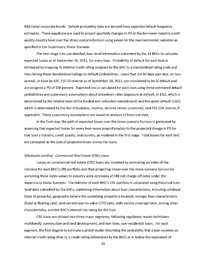
BBB-rated corporate bonds. Default probability data are derived from expected default frequency

estimates. These equations are used to project quarterly changes in PD at the borrower industry-credit

quality-country level over the stress scenario horizon using values for the macroeconomic variables as

specified in the Supervisory Stress Scenario.

The next stage is to use detailed, loan-level information submitted by the 19 BHCs to calculate

expected losses as of September 30, 2011, for every loan. Probability of default for each loan is

estimated by mapping its internal credit rating assigned by the BHC to a standardized rating scale and

then linking these standardized ratings to default probabilities. Loans that are 90 days past due, on non-

accrual, or have an ASC 310-10 reserve as of September 30, 2011, are considered to be in default and

are assigned a PD of 100 percent. Expected loss is calculated for each loan using these estimated default

probabilities and supervisory assumptions about drawdown rates (exposure at default, or EAD, which is

determined by the relative level of the funded and unfunded commitment) and loss given default (LGD),

which is determined by the line of business, country, secured versus unsecured, and FAS 114 reserve, if

applicable. These supervisory assumptions are based on analysis of historical data.

In the final step, the path of expected losses over the stress scenario horizon is generated by

assuming that expected losses for every loan move proportionately to the projected change in PD for

that loan's industry, credit quality, and country, as modeled in the first stage. Total losses for each BHC

are calculated as the sum of projected losses across the loans.

Wholesale Lending: Commercial Real Estate (CRE) Loans

Losses on commercial real estate (CRE) loans are modeled by estimating an index of the

riskiness for each BHC's CRE portfolio and then projecting losses over the stress scenario horizon by

anchoring these index values to industry-wide estimates of CRE net charge-off rates under the

Supervisory Stress Scenario. The riskiness of each BHC's CRE portfolio is calculated using historical loan-

level data submitted by the BHCs, containing information about loan characteristics, including collateral

(type of property), geography (where the underlying property is located), vintage, loan characteristics

(fixed or floating rate), and current loan-to-value (LTV) ratio, debt service coverage ratio, among other

characteristics, and the BHC's internal risk rating for the loan.

CRE loans are divided into three major segments, following regulatory report definitions:

multifamily, construction and land development, and non-farm, non-residential loans. For each

segment, the first stage is to estimate a probit model describing the probability that a loan receives an

internal credit rating (that is, a credit rating determined by the BHC) at or below the equivalent of

CCC/Caa, based on loan-level characteristics and supplemental information about the characteristics of

market (geographic location) in which the underlying property is located.

The results of these estimates are used to generate an index of the riskiness of each BHC's

multifamily, construction and land development, and non-farm, non-residential CRE portfolios, where

"riskiness" is measured as the modeled likelihood that an average dollar in the portfolio would be rated

at or below CCC/Caa. The riskiness index is calculated for each BHC's CRE portfolio as of September 30,

2011. The modeled likelihood is used in place of the actual share of dollar value loans internally rated at

or below CCC/Caa in order to capture the typical relationship between the driving variables and internal

credit quality ratings, as a way of accounting for differences across BHCs in the process and calibration

of their internal rating systems.

CRE loss rates for individual BHCs are anchored to industry-wide projections of net charge-off

rates for the banking industry as a whole under the Supervisory Stress Scenario. Specifically, each BHC's

net charge-off rate is assumed to differ from the average industry-wide rate according to its estimated

position in a modeled distribution fit to the CRE risk indices across the 19 BHCs. BHCs with risk indices

above/below the average are projected to have net charge-off rates above/below the aggregate rate to

a corresponding degree. These projected net charge-off rates are applied to loan balances in each

quarter of the stress scenario horizon (as provided by the BHCs) to generate loss amounts for the

multifamily, construction and land development, and non-farm non-residential CRE portfolios.

Retail Lending: Residential Mortgages (First Lien, HELOC, HELOANs)

Losses on residential mortgages are projected by modeling the impact of loan characteristics

and macroeconomic variables on the probability of default (PD) and on loss given default (LGD). The

first stage of this process is to use historical, loan-level data to model the probability that loans

transition to different payment statuses. These payment statuses include current, delinquent, and

default - where these are determined by the number of days a loan payment is past due - as well as

payoff (the loan is repaid). The historical data are industry-wide loan data from many banks and

mortgage loan originators. Separate transition models are estimated for three categories of closed-end

first-lien mortgages - adjustable rate, fixed rate, and option adjustable rate mortgages; home equity

lines of credit; and second-lien home equity loans. While the specific details vary by loan type, in

general the models measure the probability that a loan transitions from one payment state to another

(e.g., from current to delinquent or from delinquent to default) over a quarter, given the characteristics

of the loan, borrowers and underlying property, as well as macroeconomic variables such as local house

price growth, the statewide unemployment rate, and interest rates.

The resulting estimates are combined with industry-wide information about the characteristics

of outstanding residential mortgage loans as of September 30, 2011, and the variables defining the

Supervisory Stress Scenario to generate projections of default probabilities over the stress scenario

horizon. Outstanding loans are grouped into segments corresponding to those on the Y 14-Q regulatory

reports, including initial payment status (current or delinquent), geography, vintage, original borrower

FICO score, original LTV, and (for home equity products) combined LTV to generate segment-level

default probabilities. These segment-level default probabilities are then applied to each BHC's balances

in these segments as of September 30, 2011, as reported by the BHCs on regulatory reports. This

process generates a BHC-specific path of projected default probabilities over the stress scenario horizon.

Loss given default is calculated based on a statistical model that is estimated using historical

data for private-label mortgage-backed securities. The model takes into account the projected path of

house prices and the likely property value discount associated with distressed sales. These losses are

partitioned into those related to net charge-offs on the defaulted loans and those related to eventual

sale of the underlying property (OREO expenses).

[footnote] 23 Expenses related to OREO are included in projections of PPNR. [end of footnote.]

Changes in housing prices up until foreclosure end

(REO acquisition) are captured in LGD, while changes after foreclosure and before sale of the property

are captured in OREO expenses. The LGD for loans already in default as of September 30, 2011, includes

further home price declines through the point of foreclosure. For home equity lines of credit, balances

outstanding at the time of default (EAD) are based on the percentage of credit line drawn before

default, with higher drawn amounts assumed to result in additional draw-downs and higher exposure at

default. Taken together, the path of PD and assumed or modeled values of LGD and EAD generate a

path for losses by portfolio segment, which are aggregated to determine overall losses on the residential

mortgage loan portfolios at each BHC.

Retail Lending: Credit Cards

Losses on credit card portfolios are projected by modeling the impact of borrower and account

characteristics and macroeconomic variables on the probability of default (PD) for different type of

credit card products. The first stage of this process is to use historical, loan-level data to model the

probability that loans transition to different payment status states. These payment status states include

current, delinquent, and default - where these are determined by the number of days a loan payment is

past due. The historical data are industry-wide data from many banks. Separate transition models are

estimated for bank cards and charge cards. While the specific details vary by loan type, in general the

models measure the probability that a loan transitions from one payment state to another (e.g., from

current to delinquent or from delinquent to default) over a six-month period, given the characteristics of

the loan and borrower, as well as macroeconomic variables such as the unemployment rate.

The resulting estimates are combined with industry-wide information about the characteristics

of outstanding credit card facilities as of September 30, 2011, and the variables defining the Supervisory

Stress Scenario to generate projections of default probabilities over the stress scenario horizon. These

default rates are applied to projections of outstanding balances at the time of default, where balances

projections reflect typical balance behavior as accounts transition across payment status states (e.g.,

balance draw-downs as accounts transition from current to delinquent or from delinquent to default).

Typical balance behavior is calibrated using cross-firm data submitted by the BHCs on regulatory reports.

Finally, loss given default is the same for all BHCs but fixed by card type (bank card versus charge card),

where the loss severity rate is calibrated using data from the BHCs over a period of economic downturn

- the first quarter of 2008 to the fourth quarter of 2009.

Credit card accounts outstanding as of September 30, 2011, are grouped into segments defined

by factors such as initial payment status (current or delinquent), geography, vintage, credit line, and

borrower FICO score. Losses for each segment are generated as the product of projected

PD*LGD*outstanding balances over the stress scenario horizon for industry-wide loans in that segment.

Quarterly loss results are generated from the six-month modeled results by dividing losses for each six-

month period in half. These quarterly, segment-level loss rates are then applied to each BHC's balances

in these segments as of September 30, 2011, as reported by the BHCs on regulatory reports. This

process generates a BHC-specific path of projected loss rates over the stress scenario horizon.

Retail Lending: Auto Loans

Losses on auto loan portfolios are projected by modeling the impact of borrower and account

characteristics and macroeconomic variables on the probability of default (PD). The first stage of this

process is to use historical, loan-level data to model the probability that loans transition to default -

where default is determined by the number of days a loan payment is past due or by actions of the

borrower (bankruptcy) and the lender (repossession). The historical data are industry-wide data from

many banks and auto loan originators compiled by an industry vendor and supplemented by data

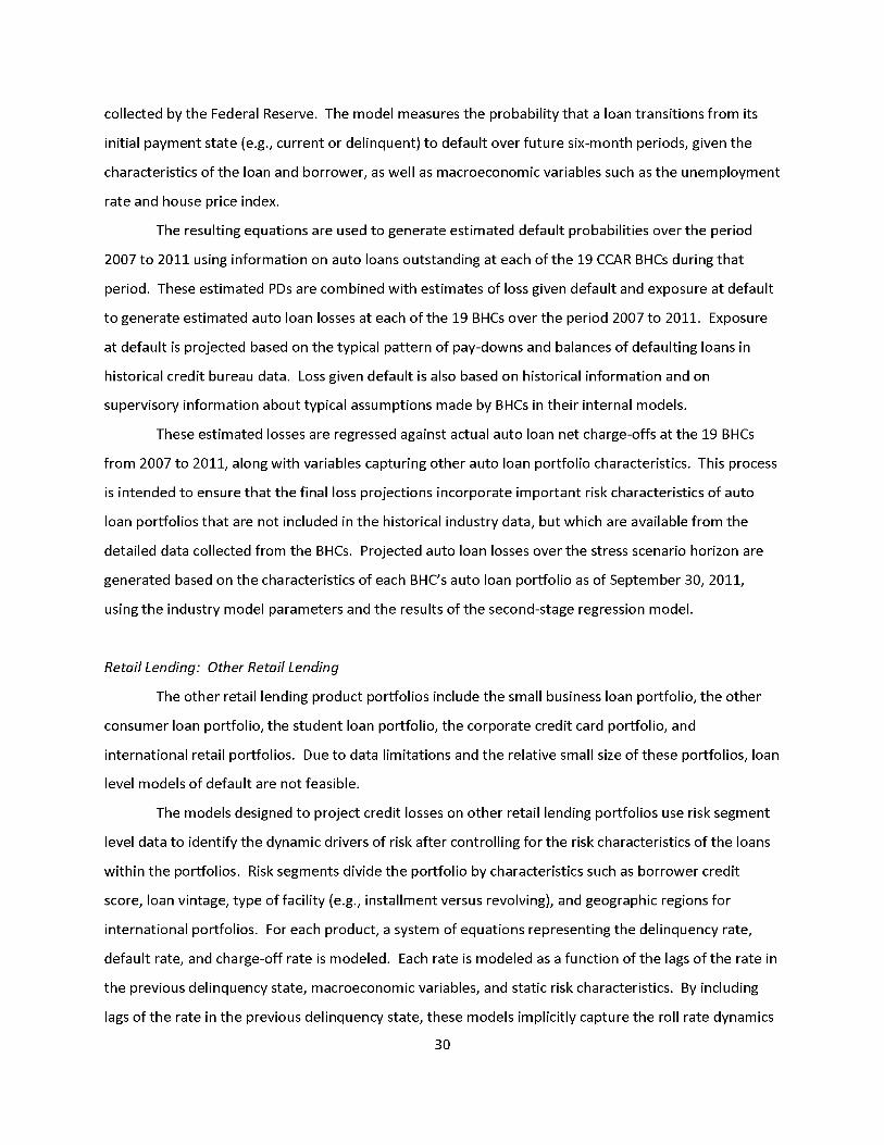
collected by the Federal Reserve. The model measures the probability that a loan transitions from its

initial payment state (e.g., current or delinquent) to default over future six-month periods, given the

characteristics of the loan and borrower, as well as macroeconomic variables such as the unemployment

rate and house price index.

The resulting equations are used to generate estimated default probabilities over the period

2007 to 2011 using information on auto loans outstanding at each of the 19 CCAR BHCs during that

period. These estimated PDs are combined with estimates of loss given default and exposure at default

to generate estimated auto loan losses at each of the 19 BHCs over the period 2007 to 2011. Exposure

at default is projected based on the typical pattern of pay-downs and balances of defaulting loans in

historical credit bureau data. Loss given default is also based on historical information and on

supervisory information about typical assumptions made by BHCs in their internal models.

These estimated losses are regressed against actual auto loan net charge-offs at the 19 BHCs

from 2007 to 2011, along with variables capturing other auto loan portfolio characteristics. This process

is intended to ensure that the final loss projections incorporate important risk characteristics of auto

loan portfolios that are not included in the historical industry data, but which are available from the

detailed data collected from the BHCs. Projected auto loan losses over the stress scenario horizon are

generated based on the characteristics of each BHC's auto loan portfolio as of September 30, 2011,

using the industry model parameters and the results of the second-stage regression model.

Retail Lending: Other Retail Lending

The other retail lending product portfolios include the small business loan portfolio, the other

consumer loan portfolio, the student loan portfolio, the corporate credit card portfolio, and

international retail portfolios. Due to data limitations and the relative small size of these portfolios, loan

level models of default are not feasible.

The models designed to project credit losses on other retail lending portfolios use risk segment

level data to identify the dynamic drivers of risk after controlling for the risk characteristics of the loans

within the portfolios. Risk segments divide the portfolio by characteristics such as borrower credit

score, loan vintage, type of facility (e.g., installment versus revolving), and geographic regions for

international portfolios. For each product, a system of equations representing the delinquency rate,

default rate, and charge-off rate is modeled. Each rate is modeled as a function of the lags of the rate in

the previous delinquency state, macroeconomic variables, and static risk characteristics. By including

lags of the rate in the previous delinquency state, these models implicitly capture the roll rate dynamics

of the different product types. The static risk characteristics of the underlying loans, such as origination

credit scores and loan-to-value ratios, are interacted with the macroeconomic variables to identify the

differences in sensitivities of the losses in different risk segments to fluctuations in the macroeconomic

variables. For each product, economic theory and the institutional characteristics of the product guide

the inclusion and lag structure of the macroeconomic variables.

Projected losses for each BHC are generated by seeding these models with the risk

characteristics of the BHC's loan portfolio as of September 30, 2011, along with lagged (actual) values of

delinquency, default, and charge-off rates and rolling the equations forward over the stress scenario

horizon.

B2. Other Losses

Securities in the AFS and HTM Portfolios

Losses on securities held in the AFS and HTM portfolios are projected other-than-temporary

impairment (OTTI) over the stress scenario horizon. Following U.S. GAAP, OTTI projections incorporate

other-than-temporary differences between amortized cost and fair market value due to credit

impairment, but not differences reflecting changes in liquidity or market conditions. Some of the

AFS/HTM securities are assumed not to be at risk for the kind of credit impairment that results in OTTI

charges, including U.S. Treasury and U.S. government agency obligations and U.S. government agency

mortgage-backed securities (MBS). The remaining securities can be grouped into two basic categories:

securitizations, where the value of the security depends on the value of an underlying pool of collateral,

and direct obligations such as corporate or sovereign bonds, where the value of the security depends

primarily on the credit quality of the issuer.

[footnote] 24 Equities are also held in the AFS and HTM portfolios, although in small amounts. Losses on these positions were calculated by applying market value shocks based on the equity prices changes in the Supervisory Stress Scenario. [end of footnote 24.]

Federal Reserve analysts developed or implemented ten

separate models to project OTTI, reflecting differences in the basic structure of the securities

(securitized versus direct obligation) and differences in underlying collateral and obligor type. Overall,

the OTTI projections involve analysis of more than 80,000 individual positions at the CUSIP level.

In general terms, the approaches used for CCAR 2012 are based on approaches used by banks

and BHCs in determining when a security is subject to an OTTI impairment charge. For securitized

obligations, credit and prepayment models estimated delinquency, default, severity, and prepayment

vectors on the underlying pool of collateral under the Supervisory Stress Scenario. In most cases, these

projections incorporate relatively detailed information on the underlying collateral characteristics for

each individual security, derived from commercial databases that contain loan-level collateral and

security structure information. Delinquency, default, severity and prepayment vectors were projected

either using econometric models developed by the Federal Reserve or industry vendor models designed

to project these estimates in stressed economic environments. These vectors were then applied to a

commercial cash flow engine that captures the specific structure of each security (e.g., tranche,

subordination, and payment rules) to calculate the intrinsic value (present value of the cash flows) for

that security. If the projected intrinsic value was less than the value at which the security is being

carried on the BHC's balance sheet (amortized cost), then the security was considered to be other than

temporarily impaired and OTTI was calculated as the difference between amortized cost and intrinsic

value.

For direct obligations, the basic approach is to assess the probability of default or severe credit

deterioration for each security issuer or group of security issuers over the stress scenario horizon.

Probability of default was either modeled directly or inferred by modeling changes in expected default

frequencies or credit default swap (CDS) spreads for the bonds in question. A security was considered to

be other than temporarily impaired if the projected value of the PD or CDS spread crossed a pre-

determined threshold level, generally the level consistent with a CCC/Caa rating, at any point during the

stress scenario horizon. Loss given default on these securities was based on historical data on bond

recovery rates. OTTI was calculated as the difference between the bond's amortized cost and its

projected value under the Supervisory Stress Scenario.

No OTTI charges are assigned to securities assumed to be acquired by the BHCs after September

30, 2011, ("incremental balances"), since these are assumed to be purchased at already discounted

prices. This assumption is also consistent with historical data showing that the composition of the AFS

and HTM portfolios tends to shift toward U.S. Treasury and agency obligations in times of economic

stress, suggesting that incremental AFS/HTM balances are less likely to be at risk of generating OTTI

charges.

Trading and Counterparty Credit Risk

The methods used to project losses on trading positions and counterparty risk exposures also

take account of the accounting treatment of these positions. Positions in the trading account are

marked to market on a daily basis, so the approach used to generate loss projections on trading

positions is intended to capture the market value impact of the global financial market shock. Total

potential losses of trading positions under a stressed market environment can be broken out into two

primary types. The first is the loss arising from a decrease in the market value of all trading positions,

regardless of the BHC's counterparties. The second is the counterparty credit risk stemming from both

changes in the size of counterparty exposures and deterioration of counterparties' creditworthiness

under stressed market conditions, which adversely affects the riskiness of positively valued trading

positions. The models used to project losses on trading positions under the global financial market

shock take account of both sources of losses.

The approach used to generate market value losses on trading positions relies on BHC estimates

of the sensitivity of the value of these positions to changes in a wide range of market rates, prices,

spreads, and volatilities. The impact of the market risk shock is calculated by multiplying these

sensitivities by the risk factor changes included in the global financial market shock developed by the

Federal Reserve. These shocks are assumed to be instantaneous and no additional hedging or changes

in positions are incorporated into the loss calculation. The resulting numbers were adjusted to take

account of positions not well captured in the data reported by the BHCs. These adjustments were based

on additional information provided by the BHCs, and the incremental losses from these sources

identified in their own global financial market shock projections, as reported in their capital plans.

The approach used to generate counterparty credit losses attempts to capture the impact of the

global financial market shock on the credit valuation adjustments (CVA) of the six BHCs with large

trading positions. CVAs are additional adjustments to the mark-to-market valuation of the BHCs' trading

portfolios to capture the impact of counterparty credit risk - the risk that a counterparty to a derivative

or other trading position will default on its obligations. These projections are made using data on

baseline and stressed exposure, loss given default (LGD), and probability of default (PD) of the

counterparty, to determine a baseline and stressed CVA. The CVA loss is the difference between the

baseline and stressed values of CVA.

In addition to capturing the impact of the global trading shock on CVAs, the models also capture

the potential additional impact of actual defaults of individual counterparties and obligors, or

incremental default-related losses (IDR) in excess of the mark-to-market losses associated with the

defaulting obligors. The models for IDR simulate loss from jump-to-default for various categories of

obligors and counterparties, grouped by product type and credit rating. IDR is an estimate of losses

from jump-to-default in the tail of the distribution of defaults, where the tail percentile was calibrated

to the shocks in the macroeconomic scenario. The model has three key components: asset correlations

that determine the correlation of obligor defaults, LGD, and the credit quality of obligors and

counterparties. For IDR on collateralized counterparty credit positions, the projections assume a margin

period of risk after the initial market shock during which no additional collateral flows are recognized

and default risk is elevated to reflect the funding stress from collateral calls.

The global financial market shock calculations for trading and counterparty positions are made

just for the six BHCs with large trading operations, largely because trading operations are a

proportionately more significant driver of risk and performance at these firms than at the other 13 BHCs

participating in CCAR 2012. Nonetheless, the Federal Reserve's projections of PPNR for all 19 BHCs

incorporate the impact of the Supervisory Stress Scenario on the revenues generated by day-to-day

trading activities such as market making for customers and clients. While the trading activities of all the

BHCs are therefore reflected in the stress scenario projections, limiting the global financial market shock

to the six with very large trading operations means that the analysis is more stringent for these BHCs in

ways that reflect the risks generated by their business activities and market focus.

Losses Related to Operational Risk Events

The model used to generate projections of operational risk losses projects operational risk

losses for the 19 BHCs as a group and then distributes these aggregate losses across the BHCs in

proportion to their Q3 2011 tier 1 common capital. This approach reflects the idiosyncratic nature of

operational risk events, as well as differences across the 19 BHCs in the way these events are captured

and reported in the data submitted to the Federal Reserve, which suggest that industry-level projections

might be more robust than firm-specific results.

The projections of industry-level operational risk losses have two primary components. The first

component projects the number of operational risk events likely to be experienced by each of the 19

BHCs under the Supervisory Stress Scenario. These projections are based on a large database collected

by the Federal Reserve of operational risk events experienced by these BHCS during the years 2004 to

2010. The data are grouped into seven categories of operational risk event types, based on the

categories used in Basel capital charges for operational risk.

[footnote] 25The seven operational risk type categories are internal fraud; external fraud; employment practices and workplace safety; clients, products and business practice; damage to physical assets; business disruption and system failure; and execution, delivery and process management. [end of footnote 25.]

The grouped data are used to calibrate

the model, along with variables that capture macroeconomic conditions and BHC-specific

characteristics. The frequency of operational risk events is projected by event type for each BHC using

the model calibrated on industry-wide data with descriptive data for the BHC and the variables in the

Supervisory Stress Scenario.

The second component of the model is an estimate of the expected severity (dollar loss) of the

operational risk events. Severity is calculated using historical operational loss data, with separate

severity estimates for each of the seven different categories of operational risk event. Operational risk

losses are generated by projecting the frequency of losses for each of the 19 BHCs under the Supervisory

Stress Scenario for each operational risk type category and then applying the corresponding severity

assumption. The operational risk losses are summed across event types and BHCs to get the aggregate

for the group. This aggregate is then re-distributed to the individual BHCs in proportion to each BHC's

tier 1 common equity as of September 30, 2011.

Loans Held for Sale or Measured Under the Fair Value Option

Certain loans are not accounted for on an accrual basis. Loans to which the fair value option

(FVO) is applied are marked to market, while loans classified as held for sale (HFS) are carried at the

lower of amortized cost or market value. These loans were identified by the BHCs in the regulatory

reports submitted as part of the CCAR process. Similar to other mark-to-market positions on the BHCs'

balance sheets (e.g., trading account positions), changes in value of these loans were calculated under

the assumptions of the global financial market shock. The specific approach varied by the type of loan.

The approach used to stress C&I loans held under FVO and HFS accounting standards was based

on a set of shocks applied to outstanding and committed C&I loan balances. Loan portfolios were

segmented based on investment grade and sub-investment grade ratings as reported by the BHCs, with

a further distinction made for the type of loan facility and amount funded. Loss rates were composed of

a shock to the funded portion net of market-value adjustments, and a shock to the remaining unfunded

portion.

The approach used to project stress losses for commercial real estate and retail loans held under

FVO and HFS accounting standards segmented exposures by major type of loan (e.g., residential

mortgages, student loans, credit cards, and the major categories of commercial real estate loans) and by

loan vintage (year of origination). Shocks consistent with the global financial market shock were applied

based on vintage and loan characteristics such as carry values and collateral, where these factors are

applicable. Residential mortgage loans under forward contract with the GSEs were generally excluded.

Mortgage Repurchase Losses

Estimates of mortgage repurchase losses for loans sold with representations and warranties

liability are based on information provided by the BHCs about the risk characteristics of loans sold to the

GSEs, into private label securities, and as whole loans. The information includes the loan vintage,

original and current unpaid balances, losses recognized to date, and current payment status, among

other measures. The model used to project mortgage repurchase losses involves two steps. The first

step is to estimate credit losses for the overall population of each BHC's sold loans with outstanding

representations and warranties liability. This step involves projecting future losses over the remaining

lifetime of the loans as well as taking account of losses recognized to date. The second step is then to

project how much of this credit loss may be ultimately put back to the selling BHC (whether through

contractual repurchase, a settlement agreement, or litigation loss).

Credit losses are projected under the home price assumptions of the Supervisory Stress Scenario

by using industry-wide information to model credit losses on various groups of mortgage loans (e.g.,

grouped by vintage and investor type). These credit loss rates were then adjusted by the credit

performance of loans sold by each BHC and mapped back to the balances of the corresponding groups

of loans reported by each BHC.

The share of credit losses likely to be ultimately put back to the selling BHCs is a difficult figure

to project, since historical information provides only limited guidance. Each investor type is evaluated

separately to determine the amount of past and future credit losses that are likely to be put back,

considering for each investor type both investor behavior to date and the procedural mechanics of

pursuing repurchase claims. For whole loans and loans sold into private label securities, the "put-back

rate," which estimates the amount of net credit losses likely to be put back to the selling BHC, is

estimated based on information from recent settlement activities in the banking industry, incorporating

adjustments for supervisory assessments of BHC-specific risk. For loans sold to the GSEs, the projected

put-back rate is based on historical information on repurchases of loans sold to the GSEs.

The projections assume that a majority but not all of the mortgage repurchase losses projected

using these techniques are realized over the nine quarters of the stress scenario horizon, with the losses

divided equally across quarters and incorporated into the PPNR projections. This assumption attempts

to balance the recognition that the resolution of repurchase issues could be a lengthy process against

the desire to ensure that the stress scenario projections incorporate a conservative assessment of the

losses to which the BHCs could be exposed over the stress scenario horizon.

B3. Pre-provision Net Revenue

In deriving projections of PPNR for each BHC under the Supervisory Stress Scenario, the Federal

Reserve leveraged multiple sources of data and information. These include historical and projected data

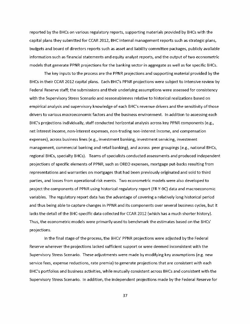
reported by the BHCs on various regulatory reports, supporting materials provided by BHCs with the

capital plans they submitted for CCAR 2012, BHC internal management reports such as strategic plans,

budgets and board of directors reports such as asset and liability committee packages, publicly available

information such as financial statements and equity analyst reports, and the output of two econometric

models that generate PPNR projections for the banking sector in aggregate as well as for specific BHCs.

The key inputs to the process are the PPNR projections and supporting material provided by the

BHCs in their CCAR 2012 capital plans. Each BHC's PPNR projections were subject to intensive review by

Federal Reserve staff; the submissions and their underlying assumptions were assessed for consistency

with the Supervisory Stress Scenario and reasonableness relative to historical realizations based on

empirical analysis and supervisory knowledge of each BHC's revenue drivers and the sensitivity of those

drivers to various macroeconomic factors and the business environment. In addition to assessing each

BHC's projections individually, staff conducted horizontal analysis across key PPNR components (e.g.,

net interest income, non-interest expenses, non-trading non-interest income, and compensation

expenses), across business lines (e.g., investment banking, investment servicing, investment

management, commercial banking and retail banking), and across peer groupings (e.g., national BHCs,

regional BHCs, specialty BHCs). Teams of specialists conducted assessments and produced independent

projections of specific elements of PPNR, such as OREO expenses, mortgage put-backs resulting from

representations and warranties on mortgages that had been previously originated and sold to third

parties, and losses from operational risk events. Two econometric models were also developed to

project the components of PPNR using historical regulatory report (FR Y-9C) data and macroeconomic

variables. The regulatory report data has the advantage of covering a relatively long historical period

and thus being able to capture changes in PPNR and its components over several business cycles, but it

lacks the detail of the BHC-specific data collected for CCAR 2012 (which has a much shorter history).

Thus, the econometric models were primarily used to benchmark the estimates based on the BHCs'

projections.

In the final stage of the process, the BHCs' PPNR projections were adjusted by the Federal

Reserve wherever the projections lacked sufficient support or were deemed inconsistent with the

Supervisory Stress Scenario. These adjustments were made by modifying key assumptions (e.g. new

service fees, expense reductions, rate premia) to generate projections that are consistent with each

BHC's portfolios and business activities, while mutually consistent across BHCs and consistent with the

Supervisory Stress Scenario. In addition, the independent projections made by the Federal Reserve for

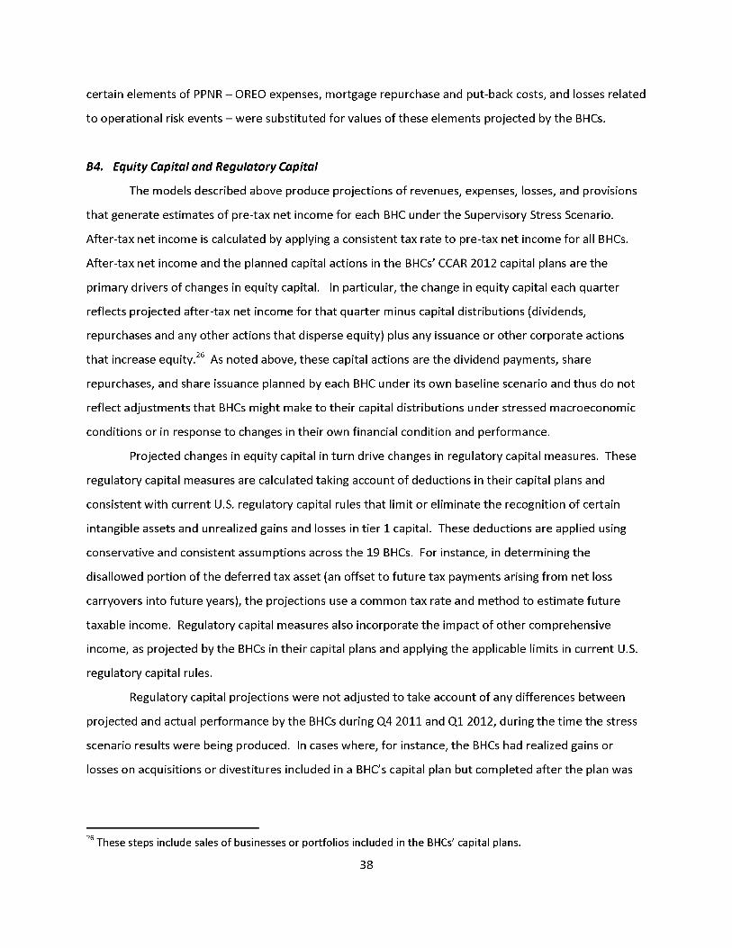
certain elements of PPNR - OREO expenses, mortgage repurchase and put-back costs, and losses related

to operational risk events - were substituted for values of these elements projected by the BHCs.

B4. Equity Capital and Regulatory Capital

The models described above produce projections of revenues, expenses, losses, and provisions

that generate estimates of pre-tax net income for each BHC under the Supervisory Stress Scenario.

After-tax net income is calculated by applying a consistent tax rate to pre-tax net income for all BHCs.

After-tax net income and the planned capital actions in the BHCs' CCAR 2012 capital plans are the

primary drivers of changes in equity capital. In particular, the change in equity capital each quarter

reflects projected after-tax net income for that quarter minus capital distributions (dividends,

repurchases and any other actions that disperse equity) plus any issuance or other corporate actions

that increase equity.

[footntoe] 26 These steps include sales of businesses or portfolios included in the BHCs' capital plans. [end of footnote 26.]

As noted above, these capital actions are the dividend payments, share

repurchases, and share issuance planned by each BHC under its own baseline scenario and thus do not

reflect adjustments that BHCs might make to their capital distributions under stressed macroeconomic

conditions or in response to changes in their own financial condition and performance.

Projected changes in equity capital in turn drive changes in regulatory capital measures. These

regulatory capital measures are calculated taking account of deductions in their capital plans and

consistent with current U.S. regulatory capital rules that limit or eliminate the recognition of certain

intangible assets and unrealized gains and losses in tier 1 capital. These deductions are applied using

conservative and consistent assumptions across the 19 BHCs. For instance, in determining the

disallowed portion of the deferred tax asset (an offset to future tax payments arising from net loss

carryovers into future years), the projections use a common tax rate and method to estimate future

taxable income. Regulatory capital measures also incorporate the impact of other comprehensive

income, as projected by the BHCs in their capital plans and applying the applicable limits in current U.S.

regulatory capital rules.

Regulatory capital projections were not adjusted to take account of any differences between

projected and actual performance by the BHCs during Q4 2011 and Q1 2012, during the time the stress

scenario results were being produced. In cases where, for instance, the BHCs had realized gains or

losses on acquisitions or divestitures included in a BHC's capital plan but completed after the plan was

developed, or in which net income was significantly different than what was projected under the

Supervisory Stress Scenario, these differences are not recognized in the stressed capital projections.

Capital ratios are calculated using total assets and risk-weighted assets based on projections

made by the BHCs as part of their CCAR 2012 capital plan submissions under the Supervisory Stress

Scenario. These projections are adjusted to account for differences between BHC and Federal Reserve

projections of certain balance sheet items, such as the ALLL and the disallowed portion of the deferred

tax asset.