CCN Interest Forwarding Strategy as Multi-Armed Bandit

HAL Id: hal-00683827https://hal.inria.fr/hal-00683827v2

Submitted on 1 Apr 2012

HAL is a multi-disciplinary open accessarchive for the deposit and dissemination of sci-entific research documents, whether they are pub-lished or not. The documents may come fromteaching and research institutions in France orabroad, or from public or private research centers.

L’archive ouverte pluridisciplinaire HAL, estdestinée au dépôt et à la diffusion de documentsscientifiques de niveau recherche, publiés ou non,émanant des établissements d’enseignement et derecherche français ou étrangers, des laboratoirespublics ou privés.

CCN Interest Forwarding Strategy as Multi-ArmedBandit Model with DelaysKonstantin Avrachenkov, Peter Jacko

To cite this version:Konstantin Avrachenkov, Peter Jacko. CCN Interest Forwarding Strategy as Multi-Armed BanditModel with Delays. [Research Report] RR-7917, INRIA. 2012. �hal-00683827v2�

https://hal.inria.fr/hal-00683827v2

https://hal.archives-ouvertes.fr

ISS

N0

24

9-6

39

9IS

RN

INR

IA/R

R--

79

17

--F

R+

EN

G

RESEARCH

REPORT

N° 7917March 2012

Project-Team Maestro

CCN Interest Forwarding

Strategy as Multi-Armed

Bandit Model with Delays

Konstantin Avrachenkov, Peter Jacko

RESEARCH CENTRE

SOPHIA ANTIPOLIS – MÉDITERRANÉE

2004 route des Lucioles - BP 93

06902 Sophia Antipolis Cedex

CCN Interest Forwarding Strategy as

Multi-Armed Bandit Model with Delays

Konstantin Avrachenkov∗, Peter Jacko†

Project-Team Maestro

Research Report n° 7917 — March 2012 — 19 pages

Abstract: We consider Content Centric Network (CCN) interest forwarding problem as a Multi-Armed Bandit (MAB) problem with delays. We investigate the transient behaviour of the ε-greedy,tuned ε-greedy and Upper Confidence Bound (UCB) interest forwarding policies. Surprisingly, forall the three policies very short initial exploratory phase is needed. We demonstrate that the tunedε-greedy algorithm is nearly as good as the UCB algorithm, the best currently available algorithm.We prove the uniform logarithmic bound for the tuned ε-greedy algorithm. In addition to itsimmediate application to CCN interest forwarding, the new theoretical results for MAB problemwith delays represent significant theoretical advances in machine learning discipline.

Key-words: Information Centric Networks, Content Centric Networks, Interest Forwarding,Multi-Armed Model with Delays

∗ INRIA Sophia Antipolis, France, [email protected]† BCAM – Basque Center for Applied Mathematics, Spain, [email protected]

Routage des Intérêts dans CCN comme le Problème de

Bandit-Manchot avec des Retards

Résumé : Nous considérons le routage des intérêts dans CCN (Content Centric Network-ing) comme le problème de bandit-manchot avec des retards. Nous etudions le comportementtransitoire des politiques : ε-greedy, tuned ε-greedy et Upper Confidence Bound (UCB). Éton-namment, pour tous les trois politiques on a besoin d’un très court première phase exploratoire.Nous démontrons que l’algorithme tuned ε-greedy est presque aussi bon que l’algorithme UCB, lemeilleur algorithme actuellement disponible. Nous établissons la limite uniforme logarithmiquepour l’algorithme tuned ε-greedy. En outre de son application immédiate au routage des in-térêts dans CCN, les nouveaux résultats théoriques pour le problème de bandit-manchot avecdes retards représentent des avancées importantes dans la discipline l’apprentissage automatique.

Mots-clés : Information Centric Networks, Content Centric Networks, Routage des Intérêts,Problème du Bandit-Manchot avec des Retards

CCN Interest Forwarding Strategy 3

1 Introduction

There is a conceptual clash between rapidly expanding digital information dissemination and thehost-based network architecture of the current Internet. To facilitate the dissemination of dig-ital information, several Information-Centric Network (ICN) architectures have been proposed:TRIAD [6], DONA [10], CCN/NDN [8]. Since the CCN/NDN (Content-Centric Networking /Named Data Networking) proposal appears to be the most elaborate, we develop our contribu-tion in the framework and within the terminology of CCN/NDN. For the sake of brevity, we shallrefer to CCN/NDN as CCN. The main features of the ICN paradigm, and the CCN architecturein particular, are that the content is addressed by a unique name and can have many identicalcached copies. Any of such copies can be retrieved independently of its location. The contentis typically divided into several small chunks. A chunk is also uniquely identified. A chunk ofcontent is located and requested by forwarding so-called interests. A user or a CCN router canforward interests to one or more neighbour CCN routers. Clearly, if there is no bandwidth limi-tation the most efficient way is to forward interests to all available neighbour routers. However, ifthere is a bandwidth limitation or the interest sender has to pay for the interest or/and deliveredcontent, there can be better interest forwarding strategies than simple flooding.

In the present work we suggest to view the problem of optimal interest forwarding strategyas a Multi-Armed Bandit (MAB) problem. The MAB problem is a classical problem in machinelearning discipline in which a decision maker finds an optimal balance between exploration andexploitation efforts. Here we adopt three well known algorithms from MAB literature: ε-greedy[12], tuned ε-greedy and UCB [1]. Our study brings advances to both networking and machinelearning disciplines. We show that the MAB algorithms allow to detect the optimal router withvery small number of interests sent to sub-optimal routers. The novelty from machine learningperspective is that we analyze the transient period of the MAB algorithms with delays. This isa very challenging topic with hardly any results available in the literature. In fact, we can onlycite the work [4] on MAB with delay. However, the model in [4] is different from ours and thereare many restrictive assumptions.

We expect that our MAB-based mechanisms can be integrated in the Interest Control Protocol(ICP) which regulates the pacing of interests [3].

The paper is organized as follows. In Section 2 we present a formal model of the problemand describe three algorithms that we propose for CCN interest forwarding. We analyze theinitial exploratory phase of these algorithms in Section 3, both numerically and mathematically,providing a bound and an approximation of its duration. In Section 4 we study the exploitationphase of the tuned ε-greedy algorithm and prove a logarithmic bound on the probability ofchoosing a suboptimal router. Section 5 concludes.

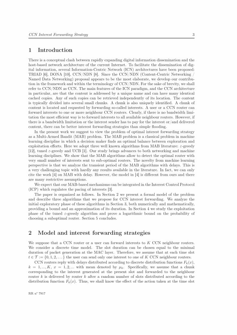
2 Model and interest forwarding strategies

We suppose that a CCN router or a user can forward interests to K CCN neighbour routers.We consider a discrete time model. The slot duration can be chosen equal to the minimalduration of packet generation at the MAC layer. Therefore, we assume that at each time slott ∈ T := {0, 1, 2, . . .} the user can send only one interest to one of K CCN neighbour routers.

CCN routers reply with delays distributed according to discrete distribution functions Fk(x),k = 1, ...,K, x = 1, 2, ... with mean denoted by µk. Specifically, we assume that a chunkcorresponding to the interest generated at the present slot and forwarded to the neighbourrouter k is delivered by router k after a random number of slots distributed according to thedistribution function Fk(x). Thus, we shall know the effect of the action taken at the time slot

RR n° 7917

4 K. Avrachenkov & P. Jacko

t only at the future time slot t + Xk(t), where Xk(t) is an i.i.d. random variable generatedaccording to Fk(x).

We are interested in minimizing the expected number of interests sent to sub-optimal routers,or to sub-optimal arms in terminology of the multi-armed bandit framework [12]. The challengingnovelty of our setting with respect to the classical multi-armed bandit problem formulation isthat the cost becomes known to the decision maker with delays. In fact, the costs are the delays.

The optimal policy in the classical setting without delay is obtained by the Gittins index rule[5], which breaks the combinatorial complexity of the problem by computing the Gittins index(a history-dependent function) for each router in isolation and then simply sending the interestat every slot to the router whose current Gittins index value is lowest. This result significantlyreduces the dimensionality of the problem, but the evaluation of the Gittins index may still becomputationally tedious, especially if the index depends on the whole history, not only on thelast observed state. Moreover, the Gittins optimality result requires that the evolution of costsfrom routers be mutually independent, while the algorithms described below are efficient evenfor dependent arms [1].

Since strictly speaking optimal policy is very likely to be very complex even in the classicalsetting without delay, many researchers have proposed sensible policies and shown desirableproperties of such policies [9, 1]. One desirable property of the multi-armed bandit problempolicy is the uniform logarithmic bound on the number of sub-optimal arms chosen by thedecision maker. We shall establish the uniform logarithmic bound for the tuned ε-greedy policyin the case of delayed information in Section 4.

In the present work we consider the following three algorithms: ε-greedy algorithm, tunedε-greedy algorithm, and UCB (Upper Confidence Bound) algorithm. These are the most usedmulti-armed bandit algorithms, and in this paper we propose their generalizations to the settingwith delayed information.

Let us formally describe each algorithm. The ε-greedy algorithm is the simplest algorithm.Its main drawback is that the expected number of sub-optimal arms grows linearly in time. Avariant of ε-greedy algorithm was proposed in [12] for Markov Decision Process models withoutdelay.

Denote by Tk(t) the total number of interests sent to router k and answered up to the end ofslot t− 1, and

Ak(τ, t) := 1{interest sent to k at τ

and answered up to the end of slot t− 1}.

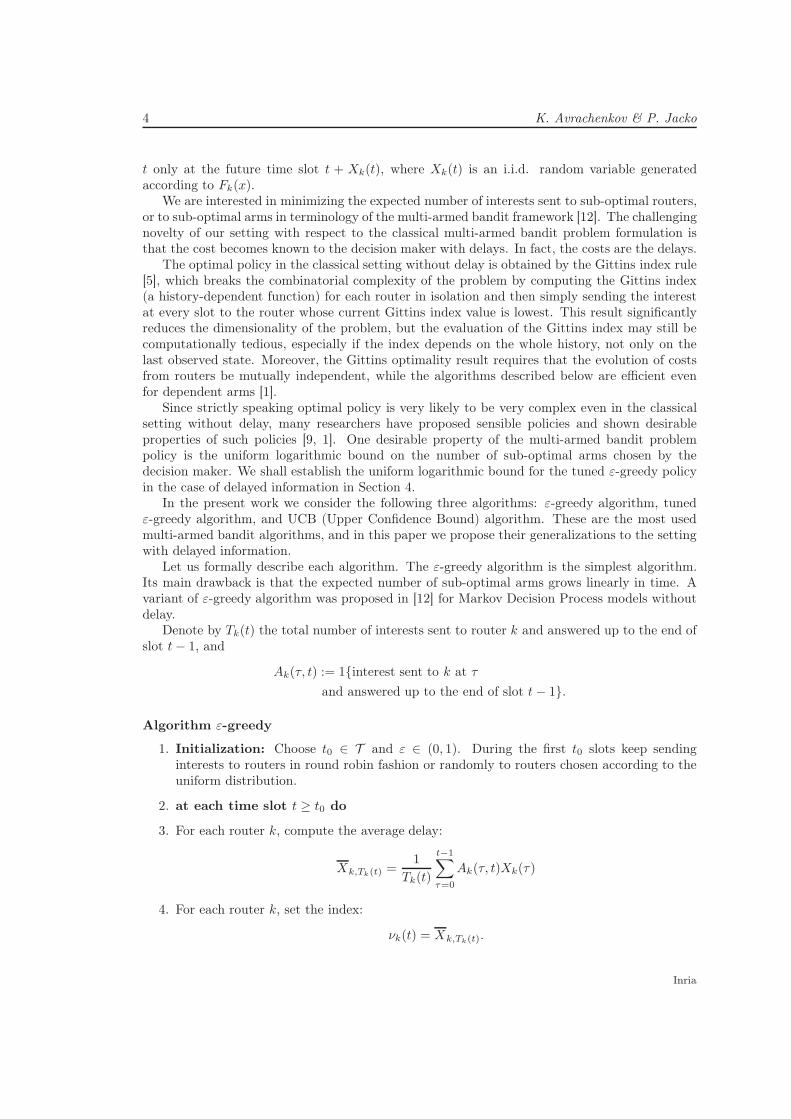
Algorithm ε-greedy

1. Initialization: Choose t0 ∈ T and ε ∈ (0, 1). During the first t0 slots keep sendinginterests to routers in round robin fashion or randomly to routers chosen according to theuniform distribution.

2. at each time slot t ≥ t0 do

3. For each router k, compute the average delay:

Xk,Tk(t) =1

Tk(t)

t−1∑

τ=0

Ak(τ, t)Xk(τ)

4. For each router k, set the index:

νk(t) = Xk,Tk(t).

Inria


5. With probability 1 − ε send new interest to the router with the smallest index or withprobability ε send new interest to a uniformly randomly chosen router.

6. end for

The tuned ε-greedy algorithm and UCB algorithm for models without delays have beenproposed and analysed in [1]. Both the tuned ε-greedy and UCB algorithms have logarithmicbounds on the number of sub-optimal arms in the case of no delays [1].

Algorithm tuned ε-greedy

1. Initialization: Choose t0 ∈ T and ε0 ∈ (0, t0). During the first t0 slots keep sendinginterests to routers in round robin fashion or randomly to routers chosen according to theuniform distribution.



Xk,Tk(t) =1

Tk(t)

t−1∑

τ=0

Ak(τ, t)Xk(τ)


νk(t) = Xk,Tk(t).

5. With probability 1− ε0/t send new interest to the router with the smallest index and withprobability ε0/t send new interest to a uniformly randomly chosen router.

6. end for

Algorithm Upper Confidence Bound (UCB)

1. Initialization: Choose t0 ∈ T and L > 0. During the first t0 slots keep sending intereststo routers in round robin fashion or randomly to routers chosen according to the uniformdistribution.



Xk,Tk(t) =1

Tk(t)

t−1∑

τ=0

Ak(τ, t)Xk(τ)


νk(t) = Xk,Tk(t) −√

L ln(t)

Tk(t)

where L is so-called exploration parameter.

5. Send new interest to the CCN router with the smallest index.

RR n° 7917


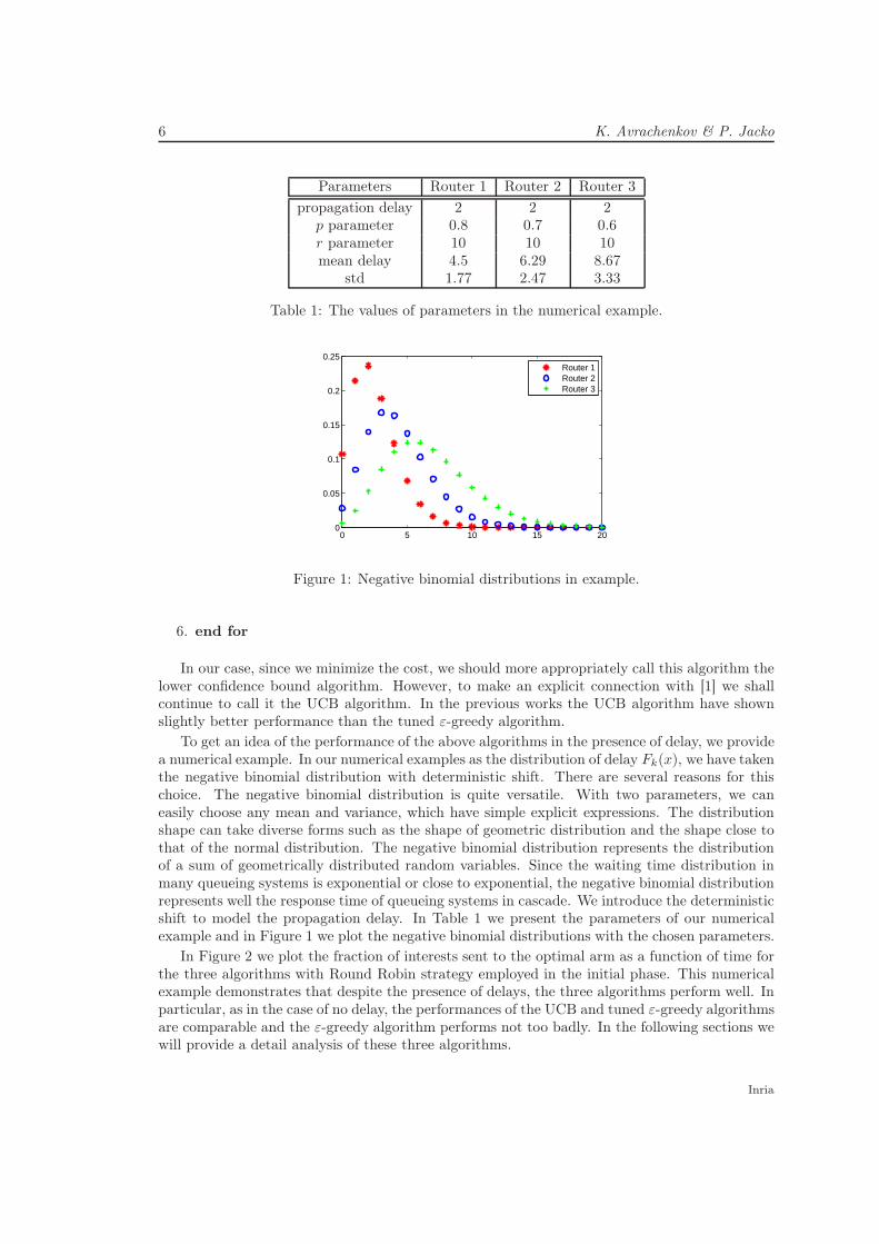
Parameters Router 1 Router 2 Router 3

propagation delay 2 2 2p parameter 0.8 0.7 0.6r parameter 10 10 10mean delay 4.5 6.29 8.67

std 1.77 2.47 3.33

Table 1: The values of parameters in the numerical example.

0 5 10 15 200

0.05

0.1

0.15

0.2

0.25

Router 1Router 2Router 3

Figure 1: Negative binomial distributions in example.

6. end for

In our case, since we minimize the cost, we should more appropriately call this algorithm thelower confidence bound algorithm. However, to make an explicit connection with [1] we shallcontinue to call it the UCB algorithm. In the previous works the UCB algorithm have shownslightly better performance than the tuned ε-greedy algorithm.

To get an idea of the performance of the above algorithms in the presence of delay, we providea numerical example. In our numerical examples as the distribution of delay Fk(x), we have takenthe negative binomial distribution with deterministic shift. There are several reasons for thischoice. The negative binomial distribution is quite versatile. With two parameters, we caneasily choose any mean and variance, which have simple explicit expressions. The distributionshape can take diverse forms such as the shape of geometric distribution and the shape close tothat of the normal distribution. The negative binomial distribution represents the distributionof a sum of geometrically distributed random variables. Since the waiting time distribution inmany queueing systems is exponential or close to exponential, the negative binomial distributionrepresents well the response time of queueing systems in cascade. We introduce the deterministicshift to model the propagation delay. In Table 1 we present the parameters of our numericalexample and in Figure 1 we plot the negative binomial distributions with the chosen parameters.

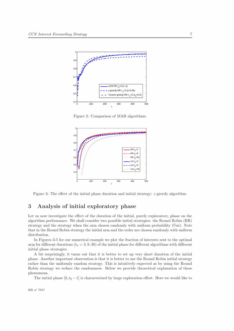
In Figure 2 we plot the fraction of interests sent to the optimal arm as a function of time forthe three algorithms with Round Robin strategy employed in the initial phase. This numericalexample demonstrates that despite the presence of delays, the three algorithms perform well. Inparticular, as in the case of no delay, the performances of the UCB and tuned ε-greedy algorithmsare comparable and the ε-greedy algorithm performs not too badly. In the following sections wewill provide a detail analysis of these three algorithms.

Inria


0 100 200 300 400 5000.4

0.5

0.6

0.7

0.8

0.9

1

t

UCB RR t0=3 (L=1)

ε-greedy RR t0=3 (ε=0.05)

Tuned ε-greedy RR t0=3 (ε

0=0.5)

Figure 2: Comparison of MAB algorithms.

0 100 200 300 400 500

0.4

0.5

0.6

0.7

0.8

0.9

1

t

RR t0=3

RR t0=9

RR t0=30

Uni t0=3

Uni t0=9

Uni t0=30

Figure 3: The effect of the initial phase duration and initial strategy: ε-greedy algorithm.

3 Analysis of initial exploratory phase

Let us now investigate the effect of the duration of the initial, purely exploratory, phase on thealgorithm performance. We shall consider two possible initial strategies: the Round Robin (RR)strategy and the strategy when the arm chosen randomly with uniform probability (Uni). Notethat in the Round Robin strategy the initial arm and the order are chosen randomly with uniformdistribution.

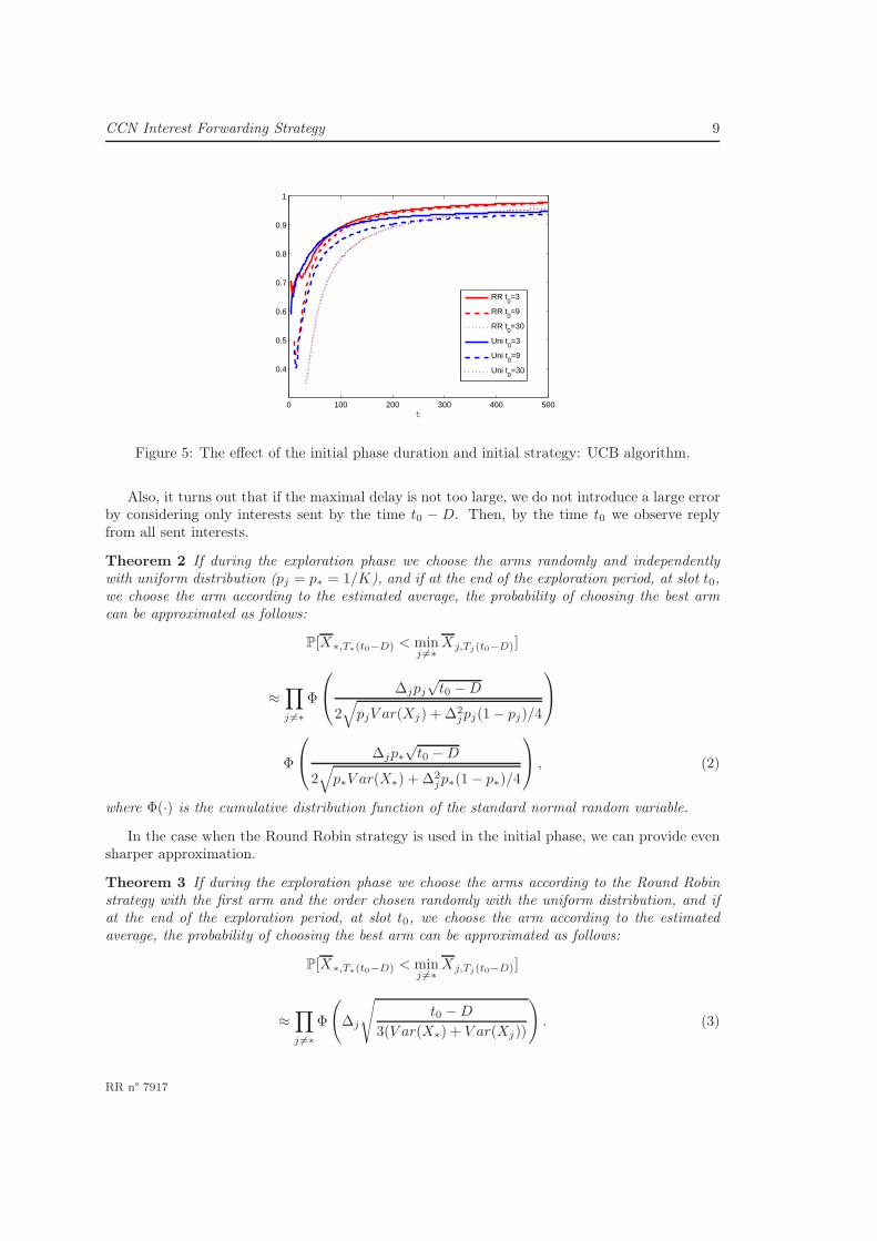
In Figures 3-5 for our numerical example we plot the fraction of interests sent to the optimalarm for different durations (t0 = 3, 9, 30) of the initial phase for different algorithms with differentinitial phase strategies.

A bit surprisingly, it turns out that it is better to set up very short duration of the initialphase. Another important observation is that it is better to use the Round Robin initial strategyrather than the uniformly random strategy. This is intuitively expected as by using the RoundRobin strategy we reduce the randomness. Below we provide theoretical explanation of thesephenomena.

The initial phase [0, t0 − 1] is characterized by large exploration effort. Here we would like to

RR n° 7917


0 100 200 300 400 500

0.4

0.5

0.6

0.7

0.8

0.9

1

t

RR t0=3

RR t0=9

RR t0=30

Uni t0=3

Uni t0=9

Uni t0=30

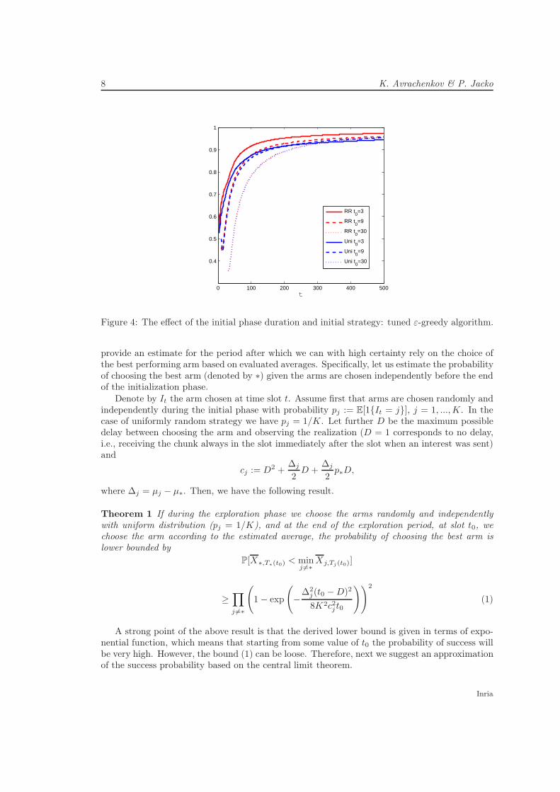
Figure 4: The effect of the initial phase duration and initial strategy: tuned ε-greedy algorithm.

provide an estimate for the period after which we can with high certainty rely on the choice ofthe best performing arm based on evaluated averages. Specifically, let us estimate the probabilityof choosing the best arm (denoted by ∗) given the arms are chosen independently before the endof the initialization phase.

Denote by It the arm chosen at time slot t. Assume first that arms are chosen randomly andindependently during the initial phase with probability pj := E[1{It = j}], j = 1, ...,K. In thecase of uniformly random strategy we have pj = 1/K. Let further D be the maximum possibledelay between choosing the arm and observing the realization (D = 1 corresponds to no delay,i.e., receiving the chunk always in the slot immediately after the slot when an interest was sent)and

cj := D2 +∆j

2D +

∆j

2p∗D,

where ∆j = µj − µ∗. Then, we have the following result.

Theorem 1 If during the exploration phase we choose the arms randomly and independentlywith uniform distribution (pj = 1/K), and at the end of the exploration period, at slot t0, wechoose the arm according to the estimated average, the probability of choosing the best arm islower bounded by

P[X∗,T∗(t0) < minj 6=∗

Xj,Tj(t0)]

≥∏

j 6=∗

(

1− exp

(

−∆2

j(t0 −D)2

8K2c2j t0

))2

(1)

A strong point of the above result is that the derived lower bound is given in terms of expo-nential function, which means that starting from some value of t0 the probability of success willbe very high. However, the bound (1) can be loose. Therefore, next we suggest an approximationof the success probability based on the central limit theorem.

Inria


0 100 200 300 400 500

0.4

0.5

0.6

0.7

0.8

0.9

1

t

RR t0=3

RR t0=9

RR t0=30

Uni t0=3

Uni t0=9

Uni t0=30

Figure 5: The effect of the initial phase duration and initial strategy: UCB algorithm.

Also, it turns out that if the maximal delay is not too large, we do not introduce a large errorby considering only interests sent by the time t0 − D. Then, by the time t0 we observe replyfrom all sent interests.

Theorem 2 If during the exploration phase we choose the arms randomly and independentlywith uniform distribution (pj = p∗ = 1/K), and if at the end of the exploration period, at slot t0,we choose the arm according to the estimated average, the probability of choosing the best armcan be approximated as follows:

P[X∗,T∗(t0−D) < minj 6=∗

Xj,Tj(t0−D)]

≈∏

j 6=∗

Φ

∆jpj√t0 −D

2√

pjV ar(Xj) + ∆2jpj(1− pj)/4

Φ

∆jp∗√t0 −D

2√

p∗V ar(X∗) + ∆2jp∗(1− p∗)/4

, (2)

where Φ(·) is the cumulative distribution function of the standard normal random variable.

In the case when the Round Robin strategy is used in the initial phase, we can provide evensharper approximation.

Theorem 3 If during the exploration phase we choose the arms according to the Round Robinstrategy with the first arm and the order chosen randomly with the uniform distribution, and ifat the end of the exploration period, at slot t0, we choose the arm according to the estimatedaverage, the probability of choosing the best arm can be approximated as follows:

P[X∗,T∗(t0−D) < minj 6=∗

Xj,Tj(t0−D)]

≈∏

j 6=∗

Φ

(

∆j

√

t0 −D

3(V ar(X∗) + V ar(Xj))

)

. (3)

RR n° 7917


10 20 30 40 50 60 70 80 90 1000

0.2

0.4

0.6

0.8

1

t0

Round Robin strategy Random strategy

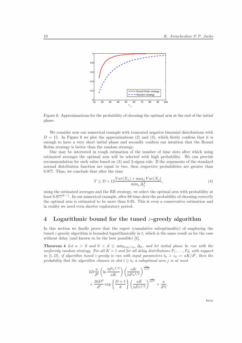
Figure 6: Approximations for the probability of choosing the optimal arm at the end of the initialphase.

We consider now our numerical example with truncated negative binomial distributions withD = 15. In Figure 6 we plot the approximations (2) and (3), which firstly confirm that it isenough to have a very short initial phase and secondly confirm our intuition that the RoundRobin strategy is better than the random strategy.

One may be interested in rough estimation of the number of time slots after which usingestimated averages the optimal arm will be selected with high probability. We can providerecommendation for such value based on (3) and 2-sigma rule. If the arguments of the standardnormal distribution function are equal to two, then respective probabilities are greater than0.977. Thus, we conclude that after the time

T ≥ D + 12V ar(X∗) + maxj V ar(Xj)

minj ∆2j

, (4)

using the estimated averages and the RR strategy, we select the optimal arm with probability atleast 0.977K−1. In our numerical example, after 68 time slots the probability of choosing correctlythe optimal arm is estimated to be more than 0.95. This is even a conservative estimation andin reality we need even shorter exploratory period.

4 Logarithmic bound for the tuned ε-greedy algorithm

In this section we finally prove that the regret (cumulative suboptimality) of employing thetuned ε-greedy algorithm is bounded logarithmically in t, which is the same result as for the casewithout delay (and known to be the best possible) [1].

Theorem 4 Let a > 0 and 0 < d ≤ mink:µk>µ∗∆k, and let initial phase be run with the

uniformly random strategy. For all K > 1 and for all delay distributions F1, . . . , FK with supportin [1, D], if algorithm tuned ε-greedy is run with input parameters t0 > ε0 := aK/d2, then theprobability that the algorithm chooses in slot t ≥ t0 a suboptimal arm j is at most

2Da

d2

(

lntd2e1/2

aK

)(

aK

td2e1/2

)3a

14d2

+16D3

d2exp

{

D + 1

8

}(

aK

td2e1/2

)a

8D2

+a

d2t.

Inria


This bound says that the cumulative probability of suboptimal decisions is logarithmic fora large enough (surely if a > max{14d2/3, 8D2}), because the instantaneous suboptimality atany slot t ≥ t0 is of the order (K − 1)a/d2t + o(1/t) for t → ∞. We conclude that the smallerthe number of arms (CCN neighbour routers) and the larger d, the difference between the meandelays of the best and the strictly second-best arm, the better is the performance of the tunedε-greedy algorithm.

5 Conclusion

The contribution of this paper is twofold. First, we have proposed tractable and well-performinginterest forwarding algorithms for CCN networks. We have demonstrated that the algorithmswork fast and logarithmically few interests are send suboptimally, which means that the resourcesof the user and CCN routers are efficiently managed. Theoretical bounds show that the learningprocess is best achievable.

Second, we have also contributed to the theory of the multi-armed bandit problem withdelayed information. This is an important and challenging topic with few existing results. Wehave provided finite-time analysis of algorithms extended to this setting and showed that thedeterioration of their performance due to delays is not significant. Perhaps surprisingly, there isno need to include a long exploratory phase, just a single datum from each arm is sufficient foran efficient performance of the algorithms.

Acknowledgement

We would like to thank Bruno Kauffmann, Luca Muscariello and Alain Simonian for stimulatingdiscussions.

References

[1] P. Auer, N. Cesa-Bianchi and P. Fischer, “Finite-time analysis of the multiarmed banditproblem”, Machine Learning, v.47, pp.235-256, 2002.

[2] G. Bennett, “Probability inequalities for the sum of independent random variables”, Journalof the American Statistical Association 57, pp. 33-45, 1962.

[3] G. Carofiglio, M. Gallo, and L. Muscariello, “ICP: Design and evaluation of an interest con-trol protocol for content-centric networking”, in Proceedings of IEEE INFOCOM Workshopon emerging design choices in name oriented networking, Orlando, USA, March 2012.

[4] S.G. Eick, “Gittins procedures for bandits with delayed responses”, Journal of the RoyalStatistical Society. Series B (Methodological), v. 50(1), pp.125-132, 1988.

[5] J.C. Gittins, “Bandit processes and dynamic allocation indices”, Journal of the Royal Sta-tistical Society, Series B, v. 41(2), pp.148-177, 1979.

[6] M. Gritter and D.R. Cheriton, “An architecture for content routing support in the internet”,in Proceedings of the USENIX Symposium on Internet Technologies and Systems, March2001.

[7] W. Hoeffding, “Probability inequalities for sums of bounded random variables”, Journal ofthe American Statistical Association 58, pp. 13-30, 1963.

RR n° 7917


[8] V. Jacobson, D. Smetters, J. Thornton, M. Plass, N. Briggs and R. Braynard, “Networkingnamed content”, in Proceedings of ACM CoNEXT 2009.

[9] T.L. Lai and H. Robbins, “Asymptotically efficient adaptive allocation rules”, Advances inApplied Mathematics, v.6(1), pp.4-22, 1985.

[10] T. Koponen, M. Chawla, B. Chun, A. Ermolinskiy, K. Kim, S. Shenker and I. Stoica, “Adata-oriented (and beyond) network architecture”, in Proceedings of ACM SIGCOMM 2007.

[11] D. Pollard, Convergence of Stochastic Processes, Springer-Verlag, 1984.

[12] R. Sutton and A. Barto, Reinforcement learning: An Introduction, MIT Press, 1998.

A Appendix: Proofs

A.1 Auxiliary Material

Let us state concentration inequalities to be used in the proofs of the theorems. We first statethe Chernoff-Hoeffding bound in a general form. This is called the Hoeffding’s inequality in [11,p. 191], citing [7].

Theorem 5 (Chernoff-Hoeffding bound) Let Y1, Y2, . . . , YT be independent random vari-ables with zero means and bounded ranges at ≤ Yt ≤ bt. Then, for each η > 0,

P[Y1 + Y2 + · · ·+ YT ≤ −η] ≤ exp

{

−2η2/

T∑

t=1

(bt − at)2

}

P[Y1 + Y2 + · · ·+ YT ≥ η] ≤ exp

{

−2η2/

T∑

t=1

(bt − at)2

}

Let us state also the Bennett’s inequality [2] and its consequence, the Bernstein’s inequality.

Theorem 6 (Bennett’s inequality) Let Y1, Y2, . . . , YT be independent random variables withzero means and bounded ranges −M ≤ Yt ≤ M . Write σ2

t for the variance of Yt. SupposeV ≥ σ2

1 + · · ·+ σ2T . Then, for each η > 0,

P[Y1 + Y2 + · · ·+ YT ≤ −η] ≤ exp

{

−1

2η2V −1B

(

MηV −1)

}

,

P[Y1 + Y2 + · · ·+ YT ≥ η] ≤ exp

{

−1

2η2V −1B

(

MηV −1)

}

,

where B(λ) := 2λ−2[(1 + λ) log(1 + λ)− λ], for λ > 0.

According to [11, p. 193]:

“The function B(·) is well-behaved: continuous, decreasing, and B(0+) = 1. Whenλ is large, B(λ) ≈ 2λ−1 logλ in the sense that the ratio tends to one as λ → ∞; theBennett Inequality does not give a true exponential bound for η compared to V/M .For smaller η it comes very close to the bound for normal tail probabilities. Problem2 shows that B(λ) ≥ (1 + 1

3λ)−1 for all λ > 0.”

Using the last bound, we get the Bernstein’s inequality.

Inria


Theorem 7 (Bernstein’s inequality) Let Y1, Y2, . . . , YT be independent random variables withzero means and bounded ranges −M ≤ Yt ≤ M . Write σ2

t for the variance of Yt. SupposeV ≥ σ2

1 + · · ·+ σ2T . Then, for each η > 0,

P[Y1 + Y2 + · · ·+ YT ≤ −η] ≤ exp

{

−1

2η2/

(

V +1

3Mη

)}

,

P[Y1 + Y2 + · · ·+ YT ≥ η] ≤ exp

{

−1

2η2/

(

V +1

3Mη

)}

.

Finally, we present the Azuma’s inequality.

Theorem 8 (Azuma’s inequality) Let Zt be a martingale with zero mean and bounded incre-ment, i.e.,

|Zt − Zt−1| ≤ c(t),

almost surely. Then, for all positive integers t and all positive reals λ, we have

P [Zt ≥ λ] ≤ exp

(

− λ2

2∑t

s=1 c2(s)

)

.

A.2 Proof of Theorem 1

We need to evaluate the following probability:

P [X̄∗,T∗(t0) < minj 6=∗

X̄j,Tj(t0)] = P [∩j 6=∗{X̄∗,T∗(t0) < X̄j,Tj(t0)}]

=∏

j 6=∗

P [X̄∗,T∗(t0) < X̄j,Tj(t0)]

≥∏

j 6=∗

P [{X̄∗,T∗(t0) < µ∗ +∆j

2} ∩ {X̄j,Tj(t0) ≥ µj −

∆j

2}]

=∏

j 6=∗

P [X̄∗,T∗(t0) < µ∗ +∆j

2]P [X̄j,Tj(t0) ≥ µj −

∆j

2]. (5)

Now let us estimate the probability P [X̄∗,T∗(t0) < µ∗ +∆j

2 ].

P [X̄∗,T∗(t0) < µ∗ +∆j

2] = 1− P [X̄∗,T∗(t0) ≥ µ∗ +

∆j

2]

= 1− P

[

∑t0s=1 1{Is = ∗}X∗(s)1{s+X∗(s) ≤ t0}∑t0

s=1 1{Is = ∗}1{s+X∗(s) ≤ t0}≥ µ∗ +

∆j

2

]

= 1− P

[

t0∑

s=1

1{Is = ∗}(X∗(s)− µ∗)1{s+X∗(s) ≤ t0} ≥ ∆j

2

t0∑

s=1

1{Is = ∗}1{s+X∗(s) ≤ t0}]

= 1− P

[

t0∑

s=1

1{Is = ∗}(X∗(s)− µ∗)1{s+X∗(s) ≤ t0}

−∆j

2

t0∑

s=1

(1{Is = ∗} − p∗)1{s+X∗(s) ≤ t0} ≥ ∆j

2p∗

t0∑

s=1

1{s+X∗(s) ≤ t0}]

RR n° 7917


= 1− P

[

t0∑

s=1

1{Is = ∗}(X∗(s)− µ∗)1{s+X∗(s) ≤ t0}

−∆j

2

t0∑

s=1

(1{Is = ∗} − p∗)1{s+X∗(s) ≤ t0} −∆j

2p∗

t0∑

s=1

(1{s+X∗(s) ≤ t0} − q∗,t0−s)

≥ ∆j

2p∗(t0 −D +

D∑

i=1

q∗,i)

]

,

where q∗,i := P [X∗(t) ≤ i].Next we define

Zj,t :=

t∑

s=1

1{Is = ∗}(X∗(s)− µ∗)1{s+X∗(s) ≤ t}

−∆j

2

t∑

s=1

(1{Is = ∗} − p∗)1{s+X∗(s) ≤ t}

−∆j

2p∗

t∑

s=1

(1{s+X∗(s) ≤ t} − q∗,t−s).

It is a martingale (with respect to the sequence of the observed delays) with zero mean andbounded increment

|Zt − Zt−1| ≤ cj ,

with cj = D2 +∆j

2 D +∆j

2 p∗D.Thus, we can apply Azuma’s inequality for martingales, which gives in our case

P [X̄∗,T∗(t0) < µ∗ +∆j

2] ≥ 1− exp

(

−∆2

j/4p2∗(t0 −D +

∑Di=1 q∗,i)

2

2c2j t0

)

≥ 1− exp

(

−∆2

j/4p2∗(t0 −D)2

2c2jt0

)

. (6)

Similarly, we have

P [X̄j,Tj(t0) ≥ µj −∆j

2] ≥ 1− exp

(

−∆2

j/4p2j(t0 −D)2

2c2jt

)

. (7)

Substituting (6) and (7) into (5), we complete the proof.


Similarly to (5), we haveP [X̄∗,T∗(t0−D) < min

j 6=∗X̄j,Tj(t0−D)]

≥∏

j 6=∗

P [X̄∗,T∗(t0−D) < µ∗ +∆j

2]P [X̄j,Tj(t0−D) ≥ µj −

∆j

2] (8)

Inria


Define

Yt =t∑

s=1

(

1{Is = ∗}(X∗,s − µ∗)−∆j

2(1{Is = ∗} − p∗)

)

.

Then, we can use the Central Limit theorem to estimate the probability

P [X̄∗,T∗(t0−D) < µ∗ +∆j

2] = P [Yt0−D <

∆j

2p∗(t0 −D)]

= P [Yt0−D

√

(t0 −D)(p∗V ar(X∗) + ∆2jp∗(1− p∗)/4)

<

∆jp∗(t0 −D)

2√

(t0 −D)(p∗V ar(X∗) + ∆2jp∗(1− p∗)/4)

],

which gives

P [X̄∗,T∗(t0−D) < µ∗ +∆j

2] ≈ Φ

∆jp∗√t0 −D

2√

p∗V ar(X∗) + ∆2jp∗(1− p∗)/4

, (9)

where Φ(·) is the standard normal distribution function. Similarly, we obtain

P [X̄j,Tj(t0−D) ≥ µj −∆j

2] ≈ Φ

∆jpj√t0 −D

2√

pjV ar(Xj) + ∆2jpj(1− pj)/4

. (10)

The substitution of (9) and (10) into (8) yields the result.

The proof of Theorem 3 is simpler than the proof of Theorem 2 and it is omitted.


Note that the assumption t ≥ t0 means that we are in the exploitation phase, and let us denoteby εt := ε0/t for all t ≥ t0, while εt := 1 for all t < t0.

Let Xj,s be the sample mean of observed delays (costs) if arm j was chosen s times conditionedon the delay distribution. Let Xj,s,u be the sample mean of observed delays if arm j was chosens times having obtained u ≤ s observations. Let Sj(t) denote the number of times arm j waschosen in the first t slots [0, t− 1]. Recall that It denotes the arm chosen at slot t. Then we have

P [It = j] ≤ (1− εt)P

[

Xj,Sj(t) ≤ maxk 6=j

Xk,Sk(t)

]

+εtK

.

Note that here we have an inequality in order to account for an arbitrary rule of breaking tiesin deciding the arm to choose in case several arms have the same lowest sample mean.

If j 6= ∗ (where ∗ denotes any of the best arms), then we can bound it by

P [It = j] ≤ P[

Xj,Sj(t) ≤ X∗,S∗(t)

]

+εtK

≤ P

[

Xj,Sj(t) ≤ µj −∆j

2

]

+ P

[

X∗,S∗(t) ≥ µ∗ +∆j

2

]

+εtK

. (11)

RR n° 7917


Let now Uj,s(t) denote the number of observed realizations by the beginning of slot t fromarm j given that it was chosen s times in the slots [0, t− 1]. In order to upperbound the first twoterms in (11) (by an expression independent of j), let us study the following expression next.

P

[

Xj,Sj(t) ≥ µj +∆j

2

]

=t∑

s=1

P

[

Sj(t) = s and Xj,s ≥ µj +∆j

2

]

=

t∑

s=1

P

[

Sj(t) = s | Xj,s ≥ µj +∆j

2

]

P

[

Xj,s ≥ µj +∆j

2

]

=

t∑

s=1

P

[


2

] s∑

u=1

P

[

Uj,s(t) = u and Xj,s,u ≥ µj +∆j

2

]

=

t∑

s=1

P

[


2

] s∑

u=1

P

[

Uj,s(t) = u | Xj,s,u ≥ µj +∆j

2

]

P

[

Xj,s,u ≥ µj +∆j

2

]

.

(12)

Assuming that P

[


2

]

> 0, then, for 1 ≤ u ≤ s,

P

[


2

]

{

= 0, if s−D + 1 > u,

≤ 1, if s−D + 1 ≤ u,

because there can be at most D− 1 unobserved realizations of the chosen arms (s− u ≤ D− 1).Hence,

s∑

u=1

P

[


2

]

P

[


2

]

≤s∑

u=max{1,s−D+1}

P

[

(Xj,s,u − µj)u ≥ ∆ju

2

]

≤s∑

u=max{1,s−D+1}

exp

{

−2

(

∆ju

2

)2

/u (2D)2

}

=

s∑

u=max{1,s−D+1}

exp

{

−(

∆2ju

8D2

)}

,

where the last inequality is due to the Chernoff-Hoeffding bound (employed with η =∆ju2 , bt =

D, at = −D,T = u).

Upperbounding the last geometric sum by a sum of constants equal to the first term, wefurther have

s∑

u=1

P

[


2

]

P

[


2

]

≤ D exp

{

−∆2

j

8D2max{1, s−D + 1}

}

.

Inria


This bound plugged into (12) therefore gives us

P

[


2

]

≤ D

t∑

s=1

P

[


2

]

exp

{

−∆2

j

8D2max{1, s−D + 1}

}

≤ D∞∑

s=1

P

[


2

]

exp

{

−∆2

j

8D2max{1, s−D + 1}

}

≤ D exp

{

−∆2

j

8D2

}

D−1∑

s=1

P

[


2

]

+D

⌊E⌋∑

s=D

P

[


2

]

exp

{

−∆2

j

8D2(s−D + 1)

}

+D

∞∑

s=⌊E⌋+1

P

[


2

]

exp

{

−∆2

j

8D2(s−D + 1)

}

(13)

where

E :=1

2K

t−1∑

s=0

εs.

Note that if ⌊E⌋ ≥ D − 1, then the above decomposition of the sum in the last step in factholds as equality. In case ⌊E⌋ < D − 1, the second term is zero and some of the summandsappear both in the first and in the third term, therefore the inequality holds.

The sum of the first and second terms in (13) can be upperbounded by

D

⌊E⌋∑

s=1

P

[


2

]

omitting the exponential terms (≤ 1), which is further upperbounded (as in [1]) by

D

⌊E⌋∑

s=1

P

[

SR

j (t) ≤ s | Xj,s ≥ µj +∆j

2

]

≤ DE P[

SR

j (t) ≤ E]

,

where SR

j (t) ≤ Sj(t) is the the number of times arm j was chosen in the first t slots [0, t − 1]at random. Using the Bernstein inequality (with Ys+1 for s = 0, 1, . . . , t − 1 being the randomvariable of sending the interest to router j at slot s, with expected value εs/K, bounded by M = 1,and variance σ2

s+1 = (1 − εs/K)(0− εs/K)2 + εs/K(1− εs/K)2 = (1 − εs/K)εs/K ≤ εs/K, sothat V = 2E, and taking η = E), we have (a slightly tighter upperbound than in [1])

P[

SR

j (t) ≤ E]

≤ exp

{

− 3

14E

}

and for t ≥ aK/d2, we lowerbound E as in [1] (denoted x0 there),

E ≥ a

d2ln

td2e1/2

aK. (14)

RR n° 7917


Therefore, the sum of the first and second terms in (13) can be upperbounded by

Da

d2

(

lntd2e1/2

aK

)(

aK

td2e1/2

)3a

14d2

.

As in [1], the third term in (13) can be upperbounded by

8D3

∆2j

exp

{

−∆2

j

8D2(⌊E⌋ −D)

}

=8D3

∆2j

exp

{

∆2j

8D2D

}

exp

{

−∆2

j

8D2⌊E⌋

}

omitting the probability term (≤ 1) and using∞∑

s=r+1

e−αs ≤ 1

αe−αr, with r = ⌊E⌋−D,α =

∆2

j

8D2 .

Further, using ⌊E⌋ ≥ E − 1, this can be upperbounded by

8D3

∆2j

exp

{

∆2j (D + 1)

8D2

}

exp

{

−∆2

j

8D2E

}

and further by

8D3

d2exp

{

D2(D + 1)

8D2

}(

aK

td2e1/2

)a

8D2

.

where the bound for the third term is obtained using (14).So, we have

P

[


2

]

≤ Da

d2

(

lntd2e1/2

aK

)(

aK

td2e1/2

)3a

14d2

+8D3

d2exp

{

D + 1

8

}(

aK

td2e1/2

)a

8D2

.

In fact, the same upperbound holds for P

[

X∗,S∗(t) ≥ µ∗ +∆j

2

]

, which is the second term in

(11).Finally, we have εt = aK/d2t to plug in the third term in (11), therefore

P [It = j] ≤ 2Da

d2

(

lntd2e1/2

aK

)(

aK

td2e1/2

)3a

14d2

+16D3

d2exp

{

D + 1

8

}(

aK

td2e1/2

)a

8D2

+a

d2t.

Inria


Contents

1 Introduction 3

2 Model and interest forwarding strategies 3

3 Analysis of initial exploratory phase 7

4 Logarithmic bound for the tuned ε-greedy algorithm 10

5 Conclusion 11

A Appendix: Proofs 12A.1 Auxiliary Material . . . . . . . . . . . . . . . . . . . . . . . . . . . . . . . . . . . 12A.2 Proof of Theorem 1 . . . . . . . . . . . . . . . . . . . . . . . . . . . . . . . . . . . 13A.3 Proof of Theorem 2 . . . . . . . . . . . . . . . . . . . . . . . . . . . . . . . . . . . 14A.4 Proof of Theorem 4 . . . . . . . . . . . . . . . . . . . . . . . . . . . . . . . . . . . 15

RR n° 7917

RESEARCH CENTRE

SOPHIA ANTIPOLIS – MÉDITERRANÉE

2004 route des Lucioles - BP 93

06902 Sophia Antipolis Cedex

Publisher

Inria

Domaine de Voluceau - Rocquencourt

BP 105 - 78153 Le Chesnay Cedex

inria.fr

ISSN 0249-6399

Documents

CCN Interest Forwarding Strategy as Multi-Armed Bandit