Embed Size (px)
Citation preview

-,- . - * -. . - . , . * . -. ,.. * . .. . . . . . . . . .
CD)iiI
~OF
A RAIN SCAVENGING MODEL FOR PREDICTING
LOW YIELD AIRBURST WEAPON FALLOUT FOROPERATIONAL TYPE STUDIES
THESIS
Curtis R. Krieser
Captain, USA
AFIT/GNE/PH/84M-9
_____________ DTICELECTE
.:Ayi2 3 1984
DEPARTMENT OF THE AIR FORCE BAIR UNIVERSITY (ATC)
AIR FORCE INSTITUTE OF TECHNOLOGY
Wright-Patterson Air Force Base, Ohio
% ~~DUTIUDUTON STATEMMN AL8 5 1 1Ap..d .i.R..J 84 05 14 119D~triutio Unlinita

, ., , i n_ n A... . .. .
AFIT/GNE/PH/84M-9
- N
": .-.
"2 A RAIN SCAVENGING MODEL FOR PREDICTING
LOW YIELD AIRBURST WEAPON FALLOUT FOR
OPERATIONAL TYPE STUDIES
THESIS
Curtis R. Krieser
Captain. USA
AFIT/GNE/PH/84M-9
DTICELECTEMAY 2 3 1984
Approved for public release; distribution unlimited" "I-B
* 4.
.°,

AFIT/GNE/PH/84M-9
.4,
A RAIN SCAVENGING MODEL FOR PREF'ICTING
LOW YIELD AIRBURST WEAPON FALLOUT FOR
OPERATIONAL TYPE STUDIES
THESIS
Presented to the Faculty of the School of Engineering
of the Air Force Institute of Technology
Air University
*, in Partial Fulfillment of the
Requirements for the Degree of
Master of Science in Nuclear Engineering
.4
Curtis R. Krieser
Captain, USA
March 1984
Approved for public release; distribution unlimited
| b
'V. Pref ace
The purpose of this study project was to develop a simple method
of predicting fallout from a low yield, nuclear airburst that would be
useful to a tactical ground commander. Simple calculation methods
exist for tactical use; however, none are utilized for airbursts. A
computer model was developed based on low yield test data. The method
produces maximum dose rate and infinite dose curves enabling a commander
to quickly identify radiation hazard areas.
I thank LCDR James H. Gogolin and Capt Arthur T. Hopkins for their
.4 contributions to the lively art of fallout conversation and providing
I constructive criticism during this study. I particularly want to express
my appreciation and thanks to Dr. Charles J. Bridgman for his guidance
and sage advice in insuring that the cart always stayed behind the horse.
Lastly, I want to thank my wife, Elsa, who always made sure that there
was a light still flickering at the end of the tunnel.
Curtis R. Krieser
Accession For
--NTIS GFA&I
DTIC TAi
RE: Classified Reference, Distribution ,tj J t -
U~nl imitedNo change per Dr. C. J. Bridgman, AFIT/ENP By
DistrtLnitiofl/Availability d S
Dist Special
.1ii "I
,,. °, ..'J

* . . . . . . . ...4- , o* • . •
Table of Contents
Page
Preface ............ ............................ i
* " List of Figures...................... v
List of Tables .......... ......................... vii
Abstract ............ ............................ viii
I. Introduction .......... ... ....................... 1
II. Types of vallout Models .......... ................. 3
Numerical Model (DELFIC) ........ .............. 3Analytical Models (WSEG and AFIT) ...... .......... 3
III. The Stabilized Nuclear Cloud ........ ............... 7
. Background ............ ..................... 7Cloud Center Height .......... ................. 7
IV. The Airburst Scavenging Model .... .............. 13
Description ........ ..................... 13Particle Size and Activity-Size Distributions 15Calculation of A(z,t) ..... ................ 19
. Fall Mechanics ................... 21
Dose Rate Calculation ..... ................ 22
V. Results .......... ......................... 28
Base Case ......... ...................... 28
Parameter Variations ..... ................ 29Summary ......... ....................... 29
VI. Conclusions and Recommendations .... ............. 40
Conclusions ........ ..................... 40Recommendations ....... ................... 40
Appendix A: Conversion of the Ground Activity Distribution
per Unit Area to a Dose Rate .. ........... 42
• Appendix B: Calculation of Atmospheric Dynamic Viscosity 46
iii
" ,"°

Page
Appendix C: The Airburst Scavenging Model Program ........ 47
Appendix D: Infinite Dose Calculations .... ............ 55
Bibliography ............ .......................... 66
Vita .............. .............................. 68
ii
5,%
.,.
-~5
S..
5.,,
.:.V -
'Vv
--5 i '* ' . . , , -" """ < -..- ' ,'' .- ¢ ' '''- " "'''' '% """.> "" ""- '

.0% List of Figures
Figure Page
1. Fallout Contour From a Constant Wind..............4
2. g(t) vs Time for a 1.0 Kiloton Surface Burst..........6
3. Cumulative Number-Size Distribution for a Surface Burst . . . 8
4. Cumulative Number Size Distribution for an Airburst........9
5. Empirical Fit to DASA 1251 Data..................12
6. g(t) vs Time for a 1.0 Kiloton Airburst..............14
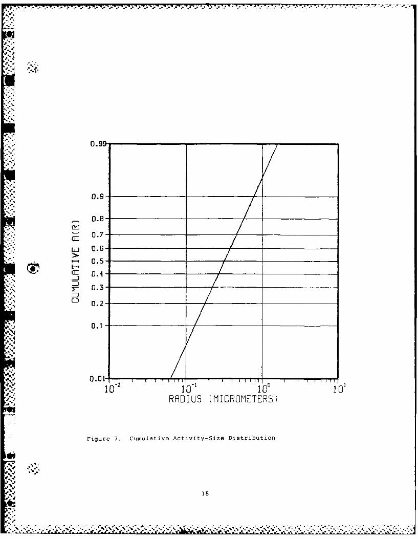
7. Cumulative Activity-Size Distribution..............18
8. Distribution of Activity with Altitude..............23
9. Distribution of Activity with Altitude.............24
10. Peak Grounded Activity.....................27
11. Maximum Dose Rate + Sigma-x Distance From a 1.0 KilotonBurst...............................30
12. Maximum Dose Rate + Sigma-x Distance From a 0.9 KilotonBurst..............................31
13. Maximum Dose Rate + Sigma-x Distance From a 0.8 KilotonBurst..............................32
14. Maximum Dose Rate + Sigma-x Distance From a 0.7 Kiloton-~ Burst ............................... 33
*15. Maximum Dose Rate + Sigma-x Distance From a 0.6 KilotonBurst..............................34
16. Maximum Dose Rate + Sigma-x Distance From a 0.5 KilotonBurst..............................35
17. Maximum Dose Rate + Sigma-x Distance From a 0.4 KilotonBurst..............................36
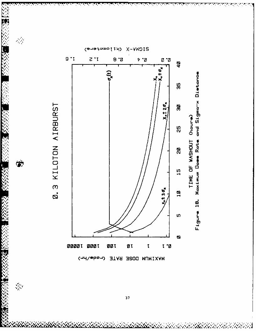
18. Maximum Dose Rate + Sigma-x Distance From a 0.3 KilotonBurst..............................37
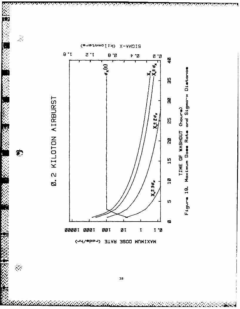
19. Maximum Dose Rate + Sigma-x Distance From a 0.2 KilotonBurst..............................38
V

Figure Page
'%'20. Maximum Dose Rate + Sigma-x Distance From a 0.1 Kiloton-Burst . . . . . . . . . . . . . . . . . . . . . . . . . . . . 39
-. 21. Point Kernal Integration Geometry . .. .. .. .. .. . .. 42
ii022. Maximum Infinite Dose and Sigma-x Distance From aS1.0 Kiloton Airburst . . . . . . . . . . . . . . . . . . . . 56
23. Maximum Infinite Dose and Sigma-x Distance From a
S24. Maximum Infinite Dose and Sigma-x Distance From a0.8 Kiloton Airburst . . . . . . . . . . . . . . . . . . . . 58
0.7 Kiloton Airburst . . . . . . . . . . . . . . . . . . . . 59
26. Maximum Infinite Dose and Sigma-x Distance From aS0.6 Kiloton Airburst . . . . . . . . . . . . . . . . . . . . 60
-
% 27. Maximum Infinite Dose and Sigma-x Distance From a
0.5 Kiloton Airburst . . . . . . . . . . . . . . . . . . . . 61
i28. Maximum Infinite Dose and Sigma-x Distance From a
:i0.4 Kiloton Airburst . . . . . . . . . . . . . . . . . . . . 62
S•29. Maximum Infinite Dose and Sigma-x Distance From a
302. Maximum Infinite Dose and Sigma-x Distance From a-' 0.2 Kiloton Airburst . . . . . . . . . . . . . . . . . . . . 64
2.31. Maximum Infinite Dose and Sigma-x Distance From a
_. ,0.1 Kiloton Airburst . . . . . . . . . . . . . . . . . . . . 659.v'
!! 20. Maximum DoseiRte Doe+ Sigma-x Distance From a0.Kion
1...0. Kiloton Airburst...................................565
...
• . .. •-.o Io . .8 Kilt on .. °. Aibrt..... ... ............... •.........5.

--,-. . . . .. . . . . . . .I77-77W7
List of Tables
.o
Table Page
I. Visible Cloud Data Extracted From DASA 1251 .. ........ 11
II. Air Burst Number-Size Distributions ... ............ 16
177. Activity-Size Groups ........ .................... 20
'4 . Base Case Parameters ........ .................... 28
vii
O4e
.,%
. / Abstract
A method was developed that enables a tactical ground commander to
predict gamma radiation dose rates and infinite doses produced by the
rain scavenging of low-yield nuclear airburst clouds. A ground activity• %".'
distribution per unit area at time t, A(xyt) , is computed using a
distribution of activity in the cloud per meter of altitude, A(zt)
To find the maximum activity grounded, it is assumed 100 percent of the
cloud activity is instantaneously deposited on the ground by the mechanism
of rain scavenging. This maximum A(x,y,t) is then converted to a maximum
dose rate, D(x,y,t), from which maximum infinite doses are computed.
Maximum dose rate and infinite dose curves vs cloud washout time (after
cloud stabilization) are presented for 10 weapon yields ranging from
1.0 kiloton to 0.1 kiloton. It is shown that the radiation hazard levels
are insignificant tactical threats at times greater than 36 hours after
cloud stabilization. -.
-%.
.4"%.,
%.,
N.,
V %
% iviii
.%
.,
. ,A RAIN SCAVENGING MODEL FOR PREDICTING
LOW YIELD AIRBURST WEAPON FALLOUT FOR
OPERATIONAL TYPE STUDIES
".-..
I. Introduction
The ability to predict fallout from the atmospheric detonation of
low yield nuclear weapons plays an important role in tactical plannino
and operations. A tactical ground commander must have the capabilit'
predict radiological contamination hazard areas resulting from the
friendly or unfriendly employment of nuclear weapons. These hazard a
are capable of producing mass casualties. Since actions must be taken
&to minimize the casualty producing effects of these hazard areas to
friendly forces, the tactical ground commander must be able to predict
the location and intensity of the hazard.
Currently a method exists that allows ground commanders to predict
fallout hazard areas for all types of nuclear weapon bursts except an
airburst (Ref 5). When an airburst is employed no tactically signifi-
cant fallout will occur because airburst fallout particles are too small
to be deposited locally on the battlefield. However, if a rain (or snow)
cloud interacts with the nuclear fallout cloud (scavenging the cloud),
then tactically significant fallout could result. A simple method use-
ful to a tactical ground commander for predicting low yield weapon fall-
out due to rain scavenging does not currently exist (Ref 6:B-12).
.O%
V.',, "-
4,
S". .. ,- ' ." -.... " -"-. ..--... . " .- .'" . .. .. -... -. .-

This thesis develops a simple rain scavenging fallout model for
the tactical commander. For the purpose of this thesis, low yields
will be defined as being less than or equal to 1 kiloton. Section Il
.. provides an introduction to the two principle types of fallout models
currently in use. Section III explains the concept of the stabilized
cloud and describes a low yield cloud model based on empirical weapons
test data. Section IV describes the rain scavenging model for airbursts.
Section V contains the results of this model and presents a method which
a tactical ground commander can use in assessing the radiological hazard
to his troops.
9.,
,._..
.•. .d-5.
*6° . •
'p4
4". 42
".5 . . . . . '5 5 *...

-. .*. II. Types of Fallout Models
This section describes the two types of fallout models presently
in use. The first type is the numerical model represented by the
Department of Defense Land Fallout Interpretive Code (DELFIC) (Ref 12).
The second type is the analytical model represented by both the Pentagon.5
-'S Weapon Systems Evaluation Group (WSEG) and Air Force Institute of Tech-
nology (AFIT) codes (Refs 14, 3).
Numerical Model (DELFIC)
DELFIC is a full physics computer code developed for use as a
research tool (Ref 12:2). DELFIC models the fallout process by comput-
ing the space-time history of fallout particles as they are transported
through the atmosphere and down toward the earth's surface. These fall-
out particles are represented by pancake shaped wafers containing distinct
%-., particle size groups. The fallout pattern on the ground at a given time
is computed by superpositioning the ground positions of those wafers
that have reached the ground in that given time. Because DELFIC must
carry out a large number of calculations, it is a slow running code and
very expensive to use. To alleviate this problem, faster running ana-
lytical codes have evolved.
Analytical models (WSEG and AFIT)
The WSEG and AFIT codes, unlike DELFIC, model the fallout particle
deposition by smearing the stabilized radioactive cloud on the ground
.-V as it falls. The resulting fallout pattern on the ground is illustratedL..' .
by the shaded area in Figure 1.
3
- %..,..*.'. %.7'

1.- 77- 71 T I
.* -.
'. ..,
.. ".4 , ..
9.4,
-%-:
Figure 1. Fallout Contour From a Constant Wind (Ref 10:2)
This smearing of the fallout cloud on the ground surface produces an
activity distribution per unit area, A(x,y,t) , that can be found from
tA(x,yt) = A (t) f f(x,y,t)g(t)dt (1)
r%_-4 where A (t) represents the total activity in the cloud at time t and4-.. t
g(t) is the fractional arrival rate of activity on the ground (Ref 3:207).
The function f(x,y,t) represents the horizontal distribution of
". activity in the cloud. It is a dual normal function with a standard
deviation in both the downwind or x direction and the crosswind or y
direction (Ref 3:208). These standard deviations are functions of the
fallout cloud arrival time on the ground, t = x/v The normalizedx
horizontal activity distribution is represented by
04
, % % ' ,' .% .' ., ... . .% - ... %%%% % % %-- '"%%: %%° . . .,.

S 1 1 _X-V t
"' .-. ;. f(x,y,t) exp2 a (t)12- t x
i exp -2 0(tv T (t) y (2)
where v is assumed to be a constant wind velocity in the x direction.x
Equation (1) is the fundamental equation used to compute fallout
footprints from smearing codes. The function g(t) is the key element of
this equation. An example of a surface burst g(t) calculation is illus-
trated in Figure 2 (Ref 3A2 ). The activity on the ground per unit
area can then be converted to a dose rate in rads per hour at a detector
3 feet off the ground
4p D(x,y,t) =C A(x,y,t) (3)
where D(x,y,t) is the dose rate and C is a constant having units of
rads per hour per unit activity per unit area (Ref 3:207). The deriva-
tion of the constant C can be found in Appendix A.
-. 5

.... ... .... ... ... .... ... .... ... ... .... -I--;.
0
0
Ci-
LL
N>
to
L0
Gn LL0600 000 ol00 00
NnCH NU ('4)

III. The Stabilized Nuclear Cloud
Background
The detonation of a nuclear weapon produces a very hot cloud of
radioactive weapon debris and incandescent air called the fireball.
This fireball rises, expands, and cools mainly by radiation convection
mixing of hot and cool air. When thermodynamic equilibrium is reached
with the ambient atmosphere, the cloud ceases to rise and becomes stabi-
lized.
In a surface burst, large amounts of surface material are lofted
into the cloud and vaporized. As the fireball cools, the radioactive
constituents become mixed and incorporated into the surface debris by
condensation. The resulting particles then fall to the earth. Figure 3
illustrates the DELFIC number-size distribution of particles resulting
from a surface burst. In an airburst, where the fireball does not inter-
sect the ground, there are no large amounts of surface debris lofted into
the cloud. As a result, the particles are much smaller and less widely
distributed in size as shown in Figure 4. These particles descend to the
earth at a much slower rate than particles produced by a surface burst
(Ref 8:36).
Cloud Center Height
The WSEG and AFIT smearing codes allow fallout particles to begin
their descent from an altitude that corresponds to the initial stabilized
cloud center height. This stabilized cloud center height is modeledo- -.
using an empirical function of the form
N*..> -*Z.... . . . . .. . . . ,.7
'P6'
AL %

0.99
..
0.7-
°Z
|'4%
LL' 0.0.99
E 0.7
4., *7 0.5ci 0.4~-J
y-- 0.3CD
0.2
0.1
/0-'% Oi.O O1* I I] IlIllI i III I I
10) 10 101 10I
RADIUS iCROf'iETE ,-I J
Figure 3. Cumulative Number-Size Distribution for a Surface Burst
8

;_ . V .;,._7 .7 7V .
,+. .,
0.99-
0.9-
0.8-
0.7-
L] 0.6-0 [.5-
a: 0.4-/-/
j- 0.3-
0.2-
0.1-
0.01-. - -2 O-' 00 1 10
R LiUS ([ICROMETERS)
40P Figure 4. Cumulative Number-Size Distribution for an Airburst
'
9
%o

, . HC = 44.0 + 6.1 inY - .205(lnY + 2.42) InY + 2.42 I (4)
where Y is the weapon yield in megatons and HC is the cloud center
4 height in kilofaet (Ref 3:213). This relation, when applied to yields
of 1 kiloton or less, produces questionable results as is pointed out in
the WSEG documentation (Ref 14:31). For example, a weapon having a 0.2
4. kiloton yield is predicted to have a stabilized cloud center height of
-0.33 kilofeet.
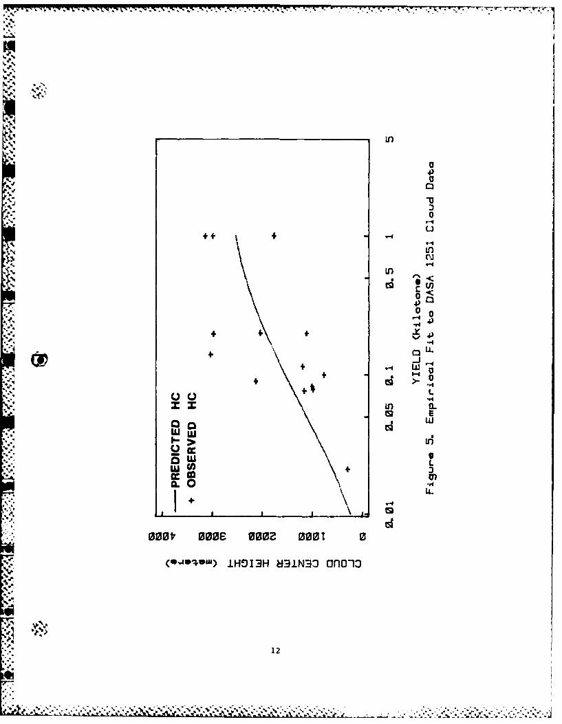
A remedy to this dilemma was to compile visible cloud data from 22
low yield airburst tests conducted between 1945 and 1962. This data was
originally compiled by the old Defense Atomic Support Agency (DASA) and
contained in its 1251 series of reports (Ref 9). The data is summarized
in Table I. A polynomial least squares fit of the data was performed to
obtain a cloud center height relation as a function of yield. It was
assumed, as in the WSEG model, that the center of the radioactive cloud
S., *is located at the same altitude as the bottom of the visible cloud
(Ref 14:24). The resulting fit is a polynomial of fourth degree having
the form
HC = 8.30476298 + .63632921 In Y - .39763749 (in Y) 2
- .01364081 (In y)3 + .00560846 (In Y)4 (5)
where Y is the weapon yield in kilotons and HC is the stabilized cloud
center height in kilofeet. Unless otherwise stated, Y will have the
4 dimensions of kilotons. Figure 5 illustrates this functional fit along'. --*,
with the data extracted from DASA 1251. It should be noted that equa-
tion (5) provides best results for yields ranging between 0.01 kilotons
10
.4...0

v... - . ,- ' W .:. .7
[4....
Table I
Visible Cloud Data Extracted From DASA 1251
SITE HEIGHT OF CLOUD BOTTOMTEST NAME YIELD ELEVATION BURST HEIGHT
(Kt) (ft) (ft) (ft MSL)
Buster Jangle-Able .1 4169.17 100.0 6700.0Tumbler Snapper-Baker 1.0 4193.0 1109.0 10000.0Upshot Knothole-Ruth .2 4000.0 304.69 10700.0Upshot Knothole-Ray .2 4026.0 180.8 7700.0Teapot-Wasp 1.0 4195.0 762.0 14500.0Teapot-Moth 2.0 4026.0 300.0 15900.0Teapot-Post 2.0 4236.0 300.0 12080.0Plumbbob-Franklin .14 4026.0 380.0 14000.8Plumbbob-Wheeler .197 4230.0 500.0 14800.0Plumbob-LaPlace 1.0 4186.0 750.0 14800.0Hardtack II-Eddy .083 4186.0 500.0 7500.0Hardtack lI-Mora 2.0 4186.0 1500.0 10000.0Hardtack 11-Hidalgo .077 4186.0 377.0 8000.0Hardtack II-Ouay .079 4249.0 100.0 75"0.6Hardtack II-Hamilton .0012 3080.0 50.0 4500.0Hardtack II-Rio Arribo .09 4010.8 72.5 11000.0Hardtack II-Wrangell .115 3077.0 1500.0 798.9Hardtack II-Catron .021 4026.0 72.5 5008.0Hardtack II-Sanford 4.9 3077.0 1500.0 12500.0Hardtack Il-Debaca 2.2 4186.0 1500.0 10000.0Hardtack II-Humboldt .0078 4029.0 25.0 6000.0Hardtack II-Santa Fe 1.3 4186.0 1580.0 13000.9
and 1.0 kiloton. Improvements to the fit can be achieved by utilizing
more test data. However, the availability of test data is limited as
recorded visible cloud data was found to be incomplete.
4.7 .4...--
'.11
tIM.
4)@
-i
U'1
o <
.~4)
:: M U .-- i
+- wov
00
+ L
Q o.0m ".4!3H 3N n7
wLUL
* I.->
+
000i 0006 M 000~ T0
(-40m.) IHOI3H 831N33 f01
12

IV. The Airburst Scavenging Model
As mentioned earlier, the key element in computing grounded fallout
activity in smearing codes is the function g(t). An illustration of
g(t) for an airburst is shown in Figure 6. This g(t) might be compared
to Figure 2 for a surface burst in Section II. It can be seen that the
airburst, with its smaller particles, leads to a steady fall over months
instead of hours. This would occur in a quiescent atmosphere. In actu-
ality, the atmosphere is very turbulent. Airburst particles may experi-
ence downdrafts, updrafts, etc. that may preclude their being grounded.
The only mechanism left for grounding of the activity is scavenging of
the radioactive cloud by rain (or snow). The conclusion to be drawn
here is that viscous fall of very small particles is a poor model for
predicting airburst fallout. Instead, rain scavenging might be a more
appropriate model. This section describes the computer model that pre-
dicts the maximum dose rate due to rain scavenging that can be encountered
for an airburst.
Description
The rain scavenging model computes the initial stabilized cloud as
described in Section III. The spatial distribution of activity in the
cloud in curies/m 3 is described by
A(x,y,z,t ) = A(z,t ) f(x) f(y) (6)5 s
where f(x) and f(y) are normalized Gaussian distributions in the x and
y directions and A(z,t ) is the vertical distribution of clouds
K 13
13

Ln
.44
.r4
-UL
U-)
"n E
-4
.4.
UL
c4d
14-

in curies/m at stabilization time t . At later times, the cloud iss
- displaced in the x direction by a constant wind of velocity v . It is
assumed that there is no y component of wind velocity. The spatial
distribution of activity is then given by
A(x,y,z,t) = A(z,t) f(x) f(y) (7)
If it is assumed a rain cloud washes out the radioactive cloud at time t
by instantaneously depositing 100 percent of the activity onto the ground,
then the horizontal distribution of activity on the ground per unit area
is described by
0
A(x,y,t) = [f A(z,t)dz] f(x) f(y) (8)z
The upper limit on the integral is taken to be zero since the integra-
- tion is carried out from the top of the cloud z (at time t) to the ground.
Particle Number-Size and Activity-Size Distributions
Section III stated that airburst particles are much smaller than
surface burst particles. Airburst particles are assumed to be spherical
C.'. in shape and obey a lognormal distribution. The number-size distribution
as a function of particle radius is expressed as
,'U 1 1 lnr-Cg0N(r) = exp 2 (9),/ 2 7, " or ( 9
:'.
.*t" where r is the particle radius in microns. The shaping parameters, ao
-8 and 8o are given bye1
".P15
i-,-

Table II
Air Burst Number-Size Distributions
GEOMETRIC STANDARD GEOMETRIC MEANDISTRIBUTION NAME DEVIATION PARTICLE RADIUS
(microns)
Norment 2.0 .075
B 1.63 .105
C 1.77 .06
D-Sample 1 1.66 .10
D-Sample 2 1.67 .09
E 2.25 .055
F 1.85 .043
G 2.16 .0325
H 1.92 .0385
.= ln(r (10)
= ln(o ) (11)
-4
where r is the geometric mean particle radius in microns and O is the
geometric standard deviation of the distribution (Ref 2). Airburst
number-size distributions have been found by Norment (Ref 13:46) and
Nathans (Ref 11:7567). The parameters for these distributions are shown
in Table II. The distribution proposed by Norment with a. = ln(.075)
and o = ln(2.0) will be used for all calculations made in this thesis.
16

* .................... *°.....-..° . . .. .
The activity-size distribution is expressed as a weighted sum of two
lognormal distributions
A(r) = f A + (1 - f )A (12)
where A is the volumetric activity-size distribution, A is the surfacev s
activity-size distribution, and f is the volumetric fractionation ratiov
of total activity (Ref 3:210). The distributions A and A are propor-v s
tional to the third and second moments of the particle size distribution
respectively. Since the nth moment of a lognormal is also a lognormal
distribution with the same value for a., the values of a can be com-
puted from the relationship given by Aitcheson and Brown (Ref 2:12).
a = a, + n (13)
Russell (Ref 16:18) has suggested that smaller particles, typical of
those found in airbursts, are often volumetrically distributed in activ-
ity. Taking this suggestion and assuming that activity in airburst
% particles is totally distributed volumetrically, f = 1.0 , equation (12)v
simplifies to
A (r ) - 1 exp -n r '3 2]
2[--8° r 2 (14)
where a3 = ln(.317) and 80 = ln(2.0) This is the activity-size
distribution that will be used in this thesis. The cumulative activity-
size distribution is shown in Figure 7.
.0017
I. " ' . " " " " ' ' ' '. ' ' ' ' ' ' " " . . . " " . " " " - . " . " = " € . . ..
,,.9
.p..
0.99
0.9-
0.8-
O7 0.7-,
C,) 0.6-
0.5ci: O.A-
0.3-0o .2-
10
RADIUS (MICROMETERSi
Figure 7. Cumulative Activity-Size Distribution
18a..-
m a"o a - - - -o.- . . ... ° . .. . . . • - • . , - - . o , ° 4 .- - - o". ,.a ' ' ' ' .- ''.' ' ' ' ' ' ' ' ' " ' ' ' , ; ' % ,, ' ' % ..- - ' ' ' ' " =, .' '' : '' -' ., , , ,, "- " . . " .'. , . . . . , -" , "- ", " " -" .

"-4
Calculation of A(z,t)
"'"' The vertical distribution of cloud activity per meter of altitude
is computed using a method developed by Bridgman and Hickman (Ref 4:2)
and is expressed as
A(z,t) = A(z,r,t)dr (15)
-f 0O
where A(z,r,t) is the specific activity in curies per vertical meter of
altitude per micron of radial size at time t. The integral in equation
(15) can be replaced by a summation over a set number of discrete activity-
a's size groups, each group containing an equal percentage of the total cloud
activity at time t, where it is assumed each group contains monosized
particles of mean radius r..hr 1
- Since the activity-size distribution shown in Figure 7 has a small
range of particle sizes, it can be divided into 10 discrete size groups,
A.(t), each having 1/10 of the total cloud activity. Table III shows the1
values of the mean particle radii for each of these activity-size groups.
Equation (15) can now be expressed as
10
A(z,t) = .10A E f .(z,t) (16)
i=ltin.
" where At is the total cloud activity and fi(z,t) is the normalized ver-
k tical activity distribution of each size group per meter of altitude at
any given time t. The total cloud activity can be expressed using the
19
'.
*Ngb,% %% , s % '. ., .' * A. .-.i .-. ,.,-... 4 r€.. .. , -'. . . ,- -a.- **%**,.-..-..-.- .. '

Table III
Activity-Size Groups
MEAN PARTICLEGROUP RADIUS
(microns)
1 .10
2 .16
3 .20
4 24
5 .29
6 .35
7 .41
8 .51
9 .65
10 .99
Way-Wigner decay formula
At = Al Y t- 1 -2 (FF) (17)
where A, is the gamma activity remaining per kiloton of fission yield
one hour after weapon detonation, Y is the weapon yield in kilotons, and
FF is the weapon fission fraction. Unless otherwise stated, FF will be
assumed to be 1.0. The value for A, is taken to be 530 gamma megacuries
per kiloton of fission (Ref 8:453). Since tissue dose rate is of inter-
S.-N est, only the gamma activity is included in the calculation. The vertical
20

distribution of cloud activity in curies/m is now expressed as
A(z,t) = 530 x l05 Y t- ~ f.(z,t) (18)10
The values of f.(z,t) are computed by assuming each size group to be
initially situated at the stabilized cloud center height, HC. Each size
* - group distribution is then allowed to fall through the atmosphere as a
fixed body until it impacts on the ground, compressing much like an
accordian.
Fall Mechanics
The fall velocity of each activity-size group can be computed
.... directly using Stoke's Law fall mechanics. Stoke's Law can be used
since the mean particle radius of each group is considerably less than
10 microns. Stoke's Law for free falling spheres in a viscous medium,
namely the atmosphere, is
46TrLivr = Tr r 3 pg (19)
where V is the dynamic viscosity of the atmosphere in kg/m-sec, v is
the particle fall velocity in m/sec, r is the particle radius in m, p
is the particle density in kg/m , and g is the gravitational accelera-
:J. tion constant which has been set to 9.8 m/sec2 The value for p is
altitude dependent. A method for calculating the dynamic viscosity
4 utilizes the US Standard Atmosphere (Ref 17) and is shown in Appendix B.
Solving for velocity gives
21
4 - %

2r 2 p g9 (1 (20)
By replacing v in equation (20) with Az/A t, the altitude of each size
group can be computed at different times t from
n
z (t) H - At (21)jol
where
n
t = A (22)j=l
The vertical distribution of cloud activity in curies/m can now be cal-
culated from
10 i z - zi(t))2
A(z,t) = 530 x 105 Yt -2 11 exp 1t)
i--i 2- 2
(23)
where a = 0.18HC , the standard deviation about the size group center
height altitude as specified in WSEG (Ref 14:51).
-.S Dose Rate Calculation
Equation (23) was evaluated at several different times. The pro-
- files are shown in Figures 8 and 9. It can be seen that for times up to
5 days after cloud stabilization, the total cloud activity three standard
deviations, a , below the distribution center height still has notz
% 22

. --
L43
43
t9 -CLU 4)
"I
4.. Lx
4)
U) 0 0r
N 'A
4
ERo 000000OO
t t
.4..
'p(04w 3ai
233
Lt.
""I 0001' f000If 00 0001 0
'

4-4
1)
0 >4
W) >. '-%- 4- 0
00
0
C1
* ci~N
00
-A.-
241

fallen below 500 m altitude. This indicates that an immersion dose due
to an airburst is not a significant threat on the ground. Since all the
cloud activity still resides in the air, equation (8) can be reduced to
A(x,y,t) = 530 x 105 Yt-1"2 f(x) f(y) (24)
Thus, equation (24) gives the ground distribution of activity per unit
area due to total cloud washout. A worst-case scenerio will allow cal-
culation of the maximum ground distribution of activity. By letting
x = v t and choosing y = 0 , y lying on the fallout footprint hot-x
line, the maximum activity grounded can be computed. The distributions
in the x direction and y direction are now simplified to
1f(x,t) =
x (25)
f(0,t) =
y (26)
These distributions are functions of time because the standard deviations
U and U are functions of time. Values for a and a are computed. x y x y
in meters using the WSEG formulae (Ref 14:50).
ax(t) - ~I 1+ 8t\ ICU xa0 T(t) a. T(27)
cZ
y(t) ;,) (z yt (28)
.5', 25
5%

where S and S represent wind shear in the x and y directions respec-x y
71 .tively. Wind shear is expressed in units of km/hr-km. By using the
assumption of a constant wind in only the x direction and a wind shear
a, only in the y direction, equation (27) simplifies to
a(t) a28t* {77~~3 (29)
The value for t* is limited to a maximum value of three hours. This
limitation is made because the second term in equations (27) and (28)
represents the toroidal growth of the cloud. This toroidal growth is
assumed to cease after three hours (Ref 4:7). Values for a are com-
puted in meters using the yield dependent relationship expressed in
WSEG (Ref 14:51)
16091exp 0.70 + (lnY) - 3.25
0 i 4.0 + (ln Y + 5.4)2 (30)
where Y is the weapon yield in megatons. The WSEG time constant, Tc
is computed in hours using WSEG's own low yield correction (Ref 15:1)
Tc -2.5 \6•J1 -. 5 exp -
12( )(11C) 2].) 2 (31)
where HC is the stabilized cloud center height in kilofeet.
The maximum dose rate can now be computed using the peak grounded
activity. This peak is illustrated in Figure 10. The dose rate is
computed by multiplying this peak grounded activity by a constant as
26
t.
... ... ;- .) :;3.,? --- )---. -- 4 ....-,
. . . . a . , ,,C * .,...
"V"
.%J.
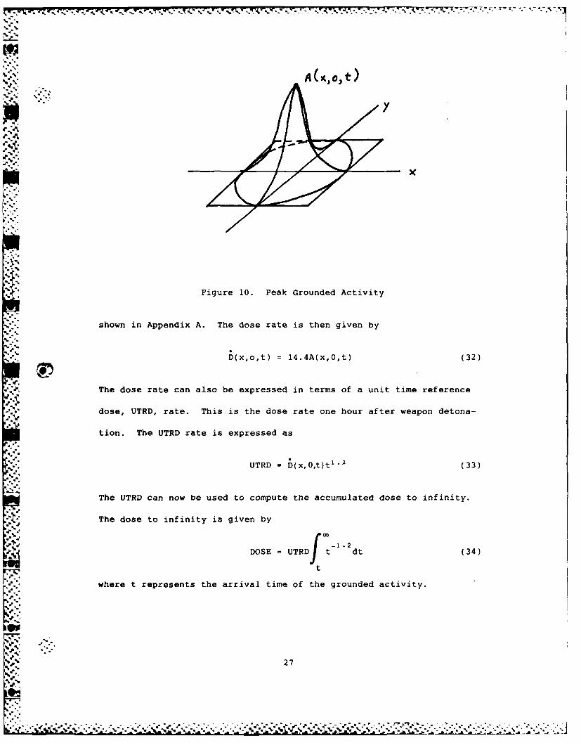
Figure 10. Peak Grounded Activity
shown in Appendix A. The dose rate is then given by
9;
D(x,o,t) = 14.4A(x,0,t) (32)
The dose rate can also be expressed in terms of a unit time reference
dose, UTRD, rate. This is the dose rate one hour after weapon detona-
tion. The UTRD rate is expressed as
UTRD = D(x,0,t)t'" (33)
The UTRD can now be used to compute the accumulated dose to infinity.
The dose to infinity is given by
DOSE = UTRD (dt 34)
t
where t represents the arrival time of the grounded activity.
V'" .- ""27

V. Results
* Base Case
A base case was established as a comparison standard. Yield was
set at 1.0 kiloton using the Norment particle number-size distribution,
ao = In (.075) and 00 = in (2.0) Fallout particle density was
chosen to be 5500 kg/m 3 (Ref 11:7565). All base case parameters are
summarized in Table IV. The cloud washout time after stabilization was
allowed to vary from 1 to 36 hours. The x coordinate of the cloud center
point was set to a value v t and then varied by factors of , 2x x #
and 3 0 . Since the f(x) distribution is a normal Gaussian, the dose
rate and dose to infinity values are symmetric about the cloud center
% point in the x direction. The results of dose rate calculations for ten
9different yields are summarized and graphically displayed in Figures 11
through 20. Infinite dose calculations for these same yields are shown
Figures 22 through 31 and can be found in Appendix D.
Table IV
Base Case Parameters
YIELD = 1.0 KILOTON
WIND SHEAR IN THE Y DIRECTION = 1.0 KM PER KM PER HOUR
DOWNWIND VELOCITY = 4.0 METERS PER SECOND
VOLUMETRIC FRACTIONATION RATIO = 1.00
PARTICLE MASS DENSITY = 5500. KILOGRAMS PER CUBIC METER
.• J ALPHAO = LN(.075) = -2.590 BETAO = LN(2.0) = .693
ALPHA2 = LN(.196) = -1.629 ALPHA3 = LN(.317) = -1.149
a%'.
28
;.. . .~- .-. -.. . . • - - .. °.- -. -. . . . . . . , ...Z. .!, . " , - % %, . - . ,

7• 7. 7.* * *- .- ~ '~
Parameter Variations
Several airburst particle number-size distributions shown in Table II
were input into the rain scavenging model. The resulting dose rates and
infinite doses reflect no change from the base case. This result is not
surprising because of the very small radii of the particles. The parti-
cles will remain aloft for many days until scavenged from the cloud, re-
gardless of the number-size distribution.
A change in particle mass density did not affect the dose rates or
infinite doses. Again, this result is not surprising for the same reason
stated above.
Downwind velocity was changed over a wind range of values. As
expected, dose rates and infinite doses did not change. Changes in down-
K. wind velocity only displace the cloud center point to different locations.
"'" Different values for wind shear in the y direction were inserted into
the model. The dose rates and infinite doses calculated did change. As
expected, a decrease in the wind shear results in an increase in the dose
rate. As wind shear decreases, less cloud activity is displaced in the
crosswind direction from the cloud center point on the ground allowing
more activity to be deposited during scavenging.
Summary
The rain scavenging model provides a simple tool useful in predict-
ing low yield, airburst fallout. A tactical ground commander need only
know local wind data, weapon yield, ground zero, and time of actual or
anticipated rain. With this information, maximum dose rates and doses
at locations upwind and downwind from the center of grounded activity
can be determined.
W .29

~W. I.'
8001 .0
@0 * 0x xin
m4
L n
Ln 0T
0 a:
/0)- LL C
0000t~~L 0~T~T~
(-'M/P~~~~) 31~30 fhIV
300

5G4-0W jH XVEI
2 *' 1 1
9. ~ 8 t0 000
bx xx
L U
/ DF- w
0D a
LU)
00
H-- E
_n L
(/H8D4 31V-4....wxv
0)1

7 - - - - 7. .-~~ . P. F. W- 7 ,
(e .J °l3UO J) X-VNSIS
. 2 T 8 70 10 0 0•I
I I I II. ~ J
0
"x Ix- xx C
(') 0
i":mE
) f.L"U
0a4"Z
N
0--. _ u 0
.- ,.[,, 0n
- E0
.. L.-/ .,
0000T 000T 001 0I T T 10
3.--1'd 3SOI InIXV.-.
32

(0e4919'wOtTUI) X-VVNOIS
9+1 *I80 V
U) m
E
0 1
0y Li) 0Xn 0
FI-0
3
I-
in L
LjL
(-/PD-) 31V8 3So0 wnflixvw
33

(esJeaWt l)X-VNOIS
x C
W m
/n 0 -
(0 N'--U
0 0LL. I-
/Lfl 0E
w 1
CO - X
'-4
344

X--W I .4
LI)
xF- t2 I
, 0-u
z00oN U)c
<- F-6
oL 0
X- E
LF)+1 HXLO 0 axI
1n L
OOOOI 000! 00! 0! T T do
(-"/PD-) 3IV8I 3600 fr'fl1ixvw
*135

2~~~ *T B 0 v* 1
C9 I
__ a
Kn 0
F- m
*L 0
A-
LULJ- C9
OOOOTOOOT 01 ol T T U
A-HOO1 31V 3SO nwxv
-' b36
(e.4eOIDIotTU-J) X-WEiIS
91 8 0 IV *0 00I I I I I I qt
b C3
x
E0 y-U
Dm 2
m wO0 N (
090, 0
'-4 w i
m HX0
t9 0
In L.20)
LL
0000001 001T 01T 1 1 00
'a (.J4j/sPcO-) 31V8 3soo wnwl~ixvw
37
-4f
x '0
F- x
U,L U)
D-'02 xx
0n (1)
K C.CC3m b
I-
Zn L03
0 LL
"4-eq*~
led .
N3
12' S0).-

.1*1
0
Ln4)m
*6
02W X
E
1z. 0 4
mm
z 31 0U.C3
on 0
1W4 E-
' -- X
00
InC.
-n L
a-..
(a4sc-' 1V SO niv
39
V; V- 7. 7. -.. .7 .
VI. Conclusions and Recommendations
Conclusions
Based on the results of this study, the following conclusions can
be drawn.
a. Utility of the model is limited to weapon yields ranging between
0.01 kilotons to 1.0 kilotons. This results from the limited low yield
visible cloud data available from atmospheric tests.
b. Fractional arrival rate of activity function, g(t), presently
used in smearing codes, is a poor model for predicting airburst fallout.
c. The immersion dose resulting from an airburst is not significant
as a ground threat.
d. Airburst fallout is only tactically significant through the
*mechanism of cloud scavenging up to 36 hours after cloud stabilization.
Recommendations
The rain scavenging model provides a useful airburst fallout pre-
diction tool; however, there is room for improvement. The following
recommendations would be appropriate for future study and are hereby
offered.
a. Compile a larger cloud data base with the intent of developing
a single yield dependent cloud center height relation useful from sub-
kiloton to megaton yields.
b. Incorporate a raindrop size distribution into the model and
begin the fallout deposition process at the time rainfall begins. The
intent is to compute a raindrop activity deposition function, g(t).
40
!.

c. Develop a method of predicting and using a "mean particle
attachment rate" of fallout particles to raindrops. This could be used
to modify the raindrop g(t) function.
","
-5.
4 .4
; -i
4 If41

Appendix A
Conversion of the Ground Activity
Distribution per Unit Area to a
Dose Rate
The ground distribution of activity per unit area, A(x,y,t) in
curies/m2 , can be converted to a dose rate in Rads/hr at a detector
3 feet off the ground. This is accomplished by doing a point kernal
integration of the gamma ray sources within the fallout field grounded
about a position having coordinates x and y at a given time t (Ref 3:207).
The geometry used for this integration is illustrated in Figure 21.
Figure 21. Point Kernal Integration Geometry
The gamma ray sources are represented as point emitters located at
points of equal differential area dA. It is assumed that the spatial
variation in A(x,y,t) away from the detector is small in terms of gamma
mean free paths. By making this assumption, the spatial variation in
P, 42
.t *%

,Alx~y,t) can be ignored and the integration taken to infinity. Addition-
S", ,-" ally, the gamma ray photons under go absorption by air molecules, are
spherically attenuated as distance away from the detector increases, and
"-.- are attenuated by one other absorbing media, namely the detector. The
'4- exposure rate at ground position x, y and at time t can now be represented
by
6(xy't) A(x,y,t) C, \c e _r tAf P 4 Tr r2 (A-1,)
0
4
.4. where
6 (x,y,t) = Exposure rate at time t (roentgens/hr)
A(x,y,t) = Ground distribution of activity (curies/m2 )
(La = Mass absorption coefficient for air (m2/kg)
= Total absorption coefficient of the detector (m
s = Distance from point emitter to detector (m)
C 1 = 3.7 x 10 1 0 disintegrations/sec-curie
C2 = 1.6 x 10- 13 joules/disintegration
C 3 = 0.00877 joules/kg-roentgen
By substituting dA = 2 7rrdr ,assuming the average gamma ray photon
energy to be 1 MeV, and using L = 0.0028 m2 /kg (Ref 7:713),
equation (A-1) reduces to
D(x,y,t) = 3.4A(x,y,t) rdr (A-2)
-'p
43i ,
'-":U
* 4 -4. - . 4.-1. . .

- - - * . . .. - .- . .* .4 - -T
where the dimensions on the constant are in roentgens per hour per unit
activity per unit area.
The above integral can be simplified further. The geometry in
Figure 21 yields:
S2 (lm)2 + r2 (A-3)
Differentiating both sides, substituting into the integral, and redef in-
ing integration limits gives:
J 2 et es d (A-4)f "0
Now, let:
tS Z (A-5)
and
ds _dz
5 z (A-6)
Substituting into equation (A-4) and simplifying gives:
'U0
eJ rdr e dz (A-7)'F.. CO f
4.. t
The integral on the right hand side of equation (A-7) is now in the form
of an Exponential Integral of the First Kind, E, ( V t ). For air, the
value of Vtis taken to be 0.0082 m -1(Ref 7:689). Substituting and
using an approximation for El (.0082) from Abramowitz and Stegun (Ref 1:231)
.*'q,'44

gives
f Gof - dz s 4.23 (A-8)
.0082
Substituting this result into equation (A-2) yields:
D(x,y,t) = 14.4A(x,y,t) (A-9)
-'4
This gives the exposure rate in roentgens per hour.
When computing the dose rate in rads per hour, the detector would
0 be human tissue rather than air. Since human tissue is comprised mainly
of water, the p value of water can be used as an approximation. The
value of the constant C 3 also changes to 0.01 joules/rad. The end result
is approximately the same as equation (A-9). Equation (A-9) can then be
used to convert a ground activity distribution per unit area to a dose
rate in rads per hour.
P
4.'
.
45
CV
4. .%'
• • • .
-• .. . . .. *'- -- , .. -'.. '.>'-? -. ,*. - ' .". -" / ,' .,.

Appendix B
Calculation of Atmospheric Dynamic Viscosity
The US Standard Atmosphere (Ref 17) provides empirical relations of
atmospheric properties as functions of altitude. These relations have
been fit to atmospheric data at various levels in the atmosphere.
,-N The largest weapon yield utilized in this thesis is 1 kiloton. The
cloud center height predicted by equation (5) for 1 kiloton is 2531 m.
For calculating the dynamic viscosity of the atmosphere, it is only
necessary to use the relations given for altitudes up to 11000 m.
The US Standard Atmosphere defines the dynamic viscosity as
1.458 x 10- 6 T 1 5
1(T) = T + 110.4 (B-1)
where T is the ambient temperature of the atmosphere in °K and pJ is in
kg/m-sec (Ref 17:19). The ambient atmospheric temperature in *K is
expressed as a function of altitude by
T(z) = 288.15 - .0065z (B-2)
where z is the altitude in m (Ref 17:10). By substituting equation (B-2)
into equation (B-i), the dynamic viscosity of the atmosphere is computed
directly from any given altitude up to 11000 m.
--v46
"."-

* .1
Appendix C
m -. ' The Airburst Scavenging Model Program
..,.k.The airburst scavenging model was written in Standard FORTRAN 77
."h
- and executed at the Air Force Institute of Technology computer facility
E . !on a DEC VAX-11/780 computer. This appendix contains the following:
~I. Program Variable Listing
" II. Listing of the Source Program7.
'.4,-
,:..,
.
.4-47
an xcte tteAi oc IsiueofTcnloycmuerfclt

4F
[,t[ -I. Program Variable Definitions
1. ALPHAO = Parameter of the particle number size distribution:logarithm of the median particle radius.
2. ALPHA2 = Parameter of the surface activity-size distribution:logarithm of the median particle radius.
3. ALPHA3 = Parameter of the volumetric activity-size distribution:logarithm of the median particle radius.
4. AXYT = Ground distribution of activity per unit area (curies/m2 ).
5. BETAO = Logarithmic slope of the particle number-size distribution.
6. CODE = An integer code used for computing different doses:Code 0 for dose to infinity, code 1 for dose to 24hours, code 2 for dose to 4 hours.
7. DDOT = Dose rate (Rads/hr).
8. DELTAT = Time step parameter set to 1.0 hours. It is used inthe Stoke's Law fall mechanics.
9. DELTAZ = Distance fallout particles fall during time DELTAT (m).
10. EXPO = Dummy variable representing the exponential argument in.°. the variable SIGO.
"A 11. EXPOFX = Dummy variable representing the exponential argument in
the variable FX.
12. EXPOFY - Dummy variable representing the exponential argument inthe variable FY.
13. DOSE = Gamma radiation dose (Rads).
14. FV = Volumetric fractionation ratio.
15. FX = Normalized Gaussian distribution in the x direction.f'p
m
16. FY = Normalized Gaussian distribution in the y direction.
17. GA Acceleration due to gravity (9.80 m/sec 2 ).
18. HC = Stabilized cloud center height (m).
19. MU Dynamic viscosity (kg/m-sec).
48

1
20. NUMBER = Dummy variable representing the squared value of SIGY.
21. PI = The mathematical constant
22. RHOP = Mass density of fallout particles (kg/m 3 ).
23. RMEAN = Vector specifying the values of mean particle radii
in each of the 10 equal activity-size groups (microns). N24. SHEARX = Wind shear in the x direction (km/hr-km).
25. SHEARY = Wind shear in the y direction (km/hr-km).
26. SIGO = Standard deviation of horizontal cloud radius (m).
27. SIGX = Cloud standard deviation in the x direction (m).
28. SIGY = Cloud standard deviation in the y direction (in).
29. SIGZ = Cloud standard deviation in the vertical direction (n).
30. TC = WSEG time constant (hours).
31. TEMP = Ambient atmospheric temperature (°K).
32. TIME = Time of cloud washout (hours).
33. TSTAR = WSEG toroidal growth time of cloud (hours).
34. UTRD = Unit time reference dose rate (Rads/hr).
35. V = Fallout particle fall velocity (m/sec).
36. VX = Wind velocity in the x-direction (m/sec).
37. VY = Wind velocity in the y-direction (m/sec).
38. XO = Cloud center position in the x-direction (m).
39. X = Distance east/west of XO (m).
40. YO = Cloud center position in the y-direction (m).
41. Y = Distance north/south of YO (m).
42. YIELD = Weapon yield (kilotons).
43. ZC = Two-dimensional array of particle size group centeraltitudes at different times of fall.
49
4 'UA

7 777-776
II. Listing of the Source Program
.50
50
* RAINOUT MODEL *
* This program computes the maximum dose rate. in Rads per hour, ** produced by a nuclear air burst. The nuclear cloud is washed out by a ** simulated r-in storm at a specified time t of cloud washout. The ** activity grounded as a result of the radioactive cloud washout, ** A(x.y.t), is used to compute the dose rate. This program will accomo- ** date changes in the following Input parameters: particle size dist-* ribution, weapon yield (for yields ranging from .01 to 1.0 kilotons), ** fractionation ratio, fallout particle density (in kilograms per cubic *, meter),wind velocity (in meters per second), and wind shear (in
kilometers per hour per kilometer of atmospheric altitude). *
REAL PI.ALPHA0.EETAO.FV.RHOP,GA.RMEAN( l0).YIELD,HC,ALPHA2.ALPHA3REAL TEMPMU.DELTAZVPRINT,XO,YO.AXYTDDOT(4),DOSE(4)REAL VSIGMAZ(10).DELTAT,ZC(IO,0:50),TIME(0:50),UTRD(4)REAL TC.SIGZ,SIG.EXPO,SIGX.TSTAPR, SIGY.NUMBERSHEARXSHEARY,VX,VYREAL X(4).Y,FX.FY.EXPOFX,EXPOFYINTEGER I.J,K.CODE.K1
C INPUT OF ALL PROBLEM PARAMETERS.
PARAMETER (PI=3.14159, ALPHAO=LOGC.075). BETA0=LOG(2.0), FV=1.0,+ RHOP=5580.0, GA=9.80. YIELD=0.1, VX=4.0, VY=0.0.+ SHEARX=10.0, SHEARY=I.0, Y=0.0. CODE=ff
OPEN (3.FILE='dosedata')REWIND 3
C SPECIFY THE MEAN PARTICLE RADII FOR THE TEN EQUAL ACTIVITY GROUPS.
,- , CALL MEAN'ALPHAO.BETAOALPHA2,ALPHA3.RMEAN)
C COMPUTE THE ALTITUDE OF THE STABILIZED CLOUD CENTER IN METERS.
HC=(1609.!5.28)*(8.30476298+.63632921*LOG(YIELD)-.39763749*LOG(YIE+LD)*LOG(YIELD)-.0l364081*LOG(YIELD)**3+.Y0560846*LOG(YIELD)**4)TC=(12.*(HC/68.)*(5.28/1609.)-2.5*(HC/60.)*(5.28/1609.)*(5.2B/1609
+ .))*(I.0-.5*EXP((HC/25.)* 5.28/1609.*!5.28/1609.)))SIGZ=.18*HCEXPO=.7+(l./3. )*LOG(YIELD/1000.)-(3.25/(..+(LOG"'CY ELD/lI00 .)+5.4)
+ *(LOG(YIELDIl000.)+5.4)))SIGZ=1609.*EXP(EXPO)
e. PRINT 1. YIELDI FORMAT (,',"YIELD = ",F6.4," KILOTON AIRBURST")PRINT 2, HC
-.' 2 FORMAT (/,"STABILIZED CLOUD CENTER HEIGHT = ",F5.0," METERS")PRINT 25, TC
25 FORMAT (/,"TC - ",F5.2," HOURS")PRINT 26, SIGO
26 FORMAT (/,"SIGMAO = ",F5.0," METERS")PRINT 27. SIGZ
27 FORMAT 1/,"SIGMAZ = ",F4.9," METERS")PRINT 28, VX
28 FORMAT .,',"DOWNWIND VELOCITY = ".F4.1," METERS PER SECOND")% PRINT 3. FV
51
%p.;RN

3 FORMAT (/,"VOLUMETRIC FRACTIONATION RATIO = ",F4.2)PRINT 35, RHOP
-;" 35 FORMAT (/,"PARTICLE MASS DENSITY = ",F5.0," KILOGRAMS PER CUBIC ME+TER")kPRINT 4, ALPHA0,BETA0
* S. 4 FORMAT (/,"ALPHA0 = LN(.075) = ",F6.3, BETAS = LN(2.0) = "4- . +F5.3)
PRINT 5, ALPHA2,ALPHA35 FORMAT (/,"ALPHA2 = LN(.196) = " F6.3," ALPHA3 = LN(.317) =+,F6.3,//)
C COMPUTE THE ALTITUDE FOR THE CENTER OF EACH PARTICLE SIZE GROUP.
DO 7 I=1,19'1," ZC(I,0)=HC
SIGMAZ(I)=.I8*ZC(I,0)'S.'7 CONTINUE
C COMPUTE THE FALL TIMES FOR EACH SIZE GROUP CENTER USING STOKE'S LAWC FALL MECHANICS.
TIME(9)=0.0DELTAT=l.0DO 13 J=1,36
TIME(J)=TIME(J-I)+DELTATDO 12 I=1,19
DELTAT=DELTAT*3600.0- TEMP=288.15-.0065*ZC(I,J-I)
MU=(1.458E-6*TEMP**i.5)/(TEMP+11.4)V=(2.0/9.Lf*((RMEAN(I)*IE-G)**2*RHOP*GA)/MUDELTAZ=V*DELTATZC(I,J)=ZC(I,3-1)-DELTAZIF(ZC(I,J).LT.0.0)THEN
ZC(I,3)=0.0GO TO 105
END IF105 DELTAT=DELTAT/3690.0
VPRINT=V*109.912 CONTINUE
- 0 13 CONTINUE
C COMPUTE THE VALUE OF THE DOSE RATE IN R/hr.
IF(CODE.EO.0)THEN---" PRINT*,'
PRINT*,'DOWNWIND SIGMAX TIME OF DOSECF + TO'." PRINT*,'DISTANCE DISTANCE WASH OUT DOSE RATE INFI
+NITY'PRINT*,' (Km) (Km) (hours) (Rads/hr) (Ra- +ds)'
PRINT*.'GO TO 200
%ELSE IF(CODE.EQ.I)THEN%. PRINT*,'
PRINT*,'DOWNWIND SIGMAX TIME OF D
.Psi +OSE TO'
.J, PRINT*,'DISTANCE DISTANCE WASH OUT DOSE RATE 2-% +4 HOURS'
-- PRINT*,' (Km) (Km) (hours) (Rads/hr)+(Rads)'
PRINT*,'GO TO 200
-- ELSE
'52
%.'eS ,5%5
•4 'A5
, ...

PRINT*.'PRINT*,'DOWNWIND SIGMAX TIME OF
+DOSE TO'44PRINT*. 'DISTANCE DISTANCE WASH OUT DOSE RATE
+4 HOURS'PRINT*.' (K(m) (K(m) (hours) (Rads/hr)
+(Rads)'-t 4 PRINT*.'-~ GO TO 200
END IF
200 DO 17 J=1.36IF(TIME( ) .LE.3.0)THEN
TSTAR=TIME(J)GO TO 135
* .. END IFTSTAR=3.Z
135 SIGX=SIGB*SORT(l.0+8.0*TSTAR/TC)NUMBER=SIGZ*SIGZ*M1.0+8.0*TSTAR/TC)+(SIlGZ*SHEARV*TIME(J))*
+ (SIGZ*SHEARY*TIME(J))SIGY=SORT(NUMBER)X0f=VX*TIME(J )*360Z.0.
'4. V0=VV*TIME(J)*3600.0'N DO 14 K=1.44 X(K)=XZ+(K-1 )*SIGX-EXPOFX=-.5*((X(K)-XZ)/SIGX)*f '(X(1()-X0/SIGX)
EXPOFV=-. 5*( (Y-V0)/SIG')*( (V-y0)/SIGy)FX=(I.0/(SQRT(2.0*PI)*SIGX))*EXP(EXPOFX)FV=(1.0/(SORT(2.Z*PI)*SIGY))*EXP(EXPOFY)AXYT=(530.E6*YIELD*TIME(.J)**(-1.2))*FX*FYDDOT( K) =14.4*AXVTUTRD(I)=DDOT(K)*TIME(J)*1I.2
4..- IF(CODE.EQ.B)THENDOSE(K)=5.0*UTRD(K)*TIME(J )**(-2)
-G GTO 14ELSE IF(COOE.EO.I)THEN
DOSE(K)=5.0*UTRD(K)*(TIMELJ )**(-2).(TIME(J)+240A)**+ (-.2))
GO TO 14ELSE
DOSE(K)=5.0*UTRD(K)*(TIME(J )**(.2)-TIME(J)+4.g)**+ (-.2))
GO TO 14END IF
14 CONTINUEA SIGX=SIGX/1000.0
WRITE (3,136,IOSTAT=K1.ERR=17) TIMECCU,.DDOT( 1),DDOT(2).DDOT(3).+ DDOT(4),DOSE'!I,DOSE(2).DOSE(3),DOSE(4),SIGX
136 FORMAT (F4. 1. X,El1.6.1XE11 .6.1X.Ell.6,lX,E11 .6,lX,Ell.6,lX.+ Ell.6.lX,E11.6,lXE11.6,1XFB.2)
PRINT 15, X,SIGX,TIME(J).DDOT.DOSE-Ni1 FORMAT (FB.3,4X,F13.3,9X,F4.1,7X.F7.2,SX.FS.2)
17 CONTINUEENOFILE (3)CLOSE (3)END
* SUBROUTINE FOR MEAN PARTICLE RADII
* 53

SUBROUTINE IEAN(ALPHAU,BETA0.ALPHAZ,ALPHA3,RMEAN)REAL ALPHAZ,BETAZ,ALPHA2,ALPHA3.Z(10),RMEAN(10)INTEGER IDATA (Z(I).I=1,12)/-l.64,-l.03,-.672,--.384,-.126..126,.384..672.
+1.03.1.641ALPHA2=ALPHAH,2.ft*BETAZ*BETA8ALPIA3=ALPHA8.3.Z*BETAft*BETA8DO 10 1=1,10
Rt4EAN( I)-EXP(Z( I)*BETAO+ALPHA3)-10 CONTINUE
RETURNEND
V 54
.i..Inint Ds Clcltin
• I°
4"..
SAq
eq,4
.-5"
-I.
']
• ."
• 4 •
55

*(se4a-,aLO T T 1) v --4 1 S
T f tj *00
Jr xW t"
L- T( LF) 0)a
ck I
x2 SI- E
LL4
0001 ~ ~ U OC O T0
'-4 T(OPOJ) 3CO 31NIJ Knix//56
2 T a1 80 00 0
41 +1
)z >i x~
.4 I x
K E
LL. HL
Z:. 41 CM .S~~ ~ 4.) i'-
* 000
LU
0)P-1 HEO3IININ~xv
3 I i57

(S~UJOT -) X-'440I S
800 0
~ 43
x
L' Tley n 0Qa
1-- 0
0I : :U) 4)
/<
1L 4 '
hIn /3 c
000001 0001 001 O1 T1 1 0
58

X +1
(eJe0w1 s -wI9t 80if)
I I I I I I I
_O 0 a
*1 +1*4)
xI E
iff
11OJ 3SO 1JI)AIvnwixvv
0 / 59

10,
'~L T
tn 8 0
a7
M 0E
0L 4 )
x
H- I
600

U' 910 10 0-0
9 b0
A 1 n 0a
0 N U) 4
X! E
OOO 00 O 0 FT0
(OP' IllO 31NAI wwx
* a'61

.51 91 8041 a
4' 4'LF)
x5'.I
0
2))
m :N' 00a
-
F- 0
Z 0o (V U) 4)F- <*1
0' *A.
x
o3Lffn
(OP-) 3600 31INIANI wnflixYN
5'.2

F- 0
0 aI-C
F- 0
N x
F- <0
0
4,- E
o
(Y))X
'-4 'L
m4 L
OOO OT OO T T 10
(SPO4) 3OO 3INIJI wnixN
63S

-. I %.
9T t'81 0 0 0
oxob CS
*3) a
x
m
L T
00
MC3z w
0 = 9~U)4
F- x*4
I--
0,
* 64SL
SL
J, 9 1 '
OOOO 000 00 *,. OT I I-*' so .-.-.-. *.*. *
(OPOaA 3SO 31NANI wnwi

810 17 * 0 0
0
4,U,
x- I- I
.44
fcn
L -0
<-' 1-.1~ ___
'# U (CI
F- <
'-4 0w
-- A
U)
07L

.
Bibliography
I. Abramowitz, Milton and Irene Stegun (Editors). Handbook of Mathemat-ical Functions (AMS 55). Washington DC: US National Bureau ofStandards, 1970.
2. Aitchison, John ana J. A. C. Brown. The Lognormal Distribution.Cambridge: Cambridge University Press, 1957.
3. Bridgman, Charles J. and Winfield S. Bigelow. "A New Fallout Predic-tion Model, " Health Physics, 43 (2): 205-218 (August 1982).
4. Bridgman, Charles J. and MAJ Burl E. Hickman. "Aircraft Penetrationsof Radioactive Clouds." Unpublished draft. School of Engineering,Air Force Institute of Technology (AU), Wright Patterson AFB OH, 1983.
5. Department of the Army. Fallout Prediction. FM 3-22. Washington:HQ USA, 30 October 1973.
6. Department of the Army. Staff Officer's Field Manual Nuclear WeaponsEmployment Doctrine and Procedures. FM 101-31-1. Washington: HQUSA, 21 March 1977.
7. Evans, R. D. The Atomic Nucleus. New York: McGraw-Hill Book Com-pany, 1955.
8. Glasstone, Samuel and Philip J. Dolan. The Effects of Nuclear Weapons(Third Edition). Washington DC: United States Department of Defense,United States Energy Research and Development Administration, March
1977.
9. Hawthorne, Howard A. (Editor). Compilation of Local Fallout DataFrom Test Detonations 1945-1962 Extracted From DASA 1251. Volume I-Continental US Tests, Report Number DNA 1251-I-EX, Defense NuclearAgency, Washington DC, May 1979 (AD-A079 309).
10. Hopkins, Capt Arthur T. A Two Step Method To Treat Variable Windsin Fallout Smearing Codes. MS Thesis, GNE/PH/82M-10. School ofEngineering, Air Force Institute of Technology (AU), Wright-PattersonAFB OH, March 1982 (AD-Ail5 514).
11. Nathans, M. W. and others. "Particle Size Distributions in CloudsFrom Nuclear Airbursts," Journal of Geophysical Research, 75 (36):
7559-7572 (December 1970).
12. Norment, Hillyer G. Department of Defense Land Fallout PredictionSystem. Volume I-System Description, Report Number DASA-1800-I,
Defense Atomic Support Agency, Washington DC, June 1966 (AD 483 897)..0
66
,S.. -'-;..... ,..........v.".".",-...-.-.. '" -" . ' J : " L"' " - ¢. "

13. Norment, Hillyer G. A Precipitation Scavaging Model for Studies ofTactical Nuclear Operations. Volume I-Theory and Preliminary
-., Results. Report Number DNA 3661F-1, Defense Nuclear Agency, Wash-% "ington DC, June 1975 (AD-A014 960).
14. Pugh, George E. and Robert J. Galiano. An Analytic Model of Close-
, In Deposition of Fallout for Use In Operational Type Studies. WSEG
Research Memorandum No. 10, Washington DC: Weapon Systems Evalua-A tion Group, The Pentagon, October 1959 (AD 261 752).
15. ------- Revision of Fallout Parameters for Low Yield Detonations.Supplement to WSEG Research Memorandum No. 10, Washington DC:Weapon Systems Evaluation Group, The Pentagon, October 1961
(AD-061 536).
16. Russell, Irving. Critique of Land Fallout Models (U). Report NumberAFWL-TR-65-76, US Air Force Weapons Laboratory, Kirtland AFB NM,February 1966, (SECRET RESTRICTED DATA) (AD 371 832).
17. US Standard Atmosphere, 1976. Washington DC: National Oceanic and
Atmospheric Administration, National Aeronautics and Space Adminis-
tration, United States Air Force, October 1976.
I°
% ,
.
67

VITA
Curtis Randall Krieser was born in
~* the son of R. a and -. He grad-
uated from Homewood-Flossmoor High School in 1970. In December 1974,
he graduated from the University of Illinois with a Bachelor of Science
degree in Engineering Physics and was commissioned a second lieutenant
in the United States Army through the ROTC program. He attended theIOrdnance Officer's Basic Course at Aberdeen Proving Ground, Maryland,
the Missile Maintenance Officer's Course at Redstone Arsenal, Alabama,
and the Airborne Course at Fort Benning, Georgia. In October 1975 he
was assigned to the 525th Ordnance Company in Siegelsbach, West Germany.
He returned to Redstone Arsenal in September 1979 to attend the Ord-
nance Officer's Advanced Course. In May 1930 he was assigned to Fort
Bliss, Texas where he commanded the Maintenance Battery, 2d Battalion
(Nike Hercules) 52d Air Defense Artillery. He entered the Air Force
Institute of Technology Nuclear Engineering Program in August 1982.
He and his wife J have and P .
Permanent address _
68

UNCLASSIFIEDSECURITY CLASSIFICATION OF THIS PAGE
I REPORT DOCUMENTATION PAGEIREPORT SECURITY CLASSIFICATION 1b. RESTRICTIVE MARKINGS
UNCLASSIFIEDSECURITY-CLASSIFICATION____AUTHORITY 3. DSRBTO/VIALTYOF REPORT
4. PERFORMING ORGANIZATION REPORT NUMBER(S) 5. MONITORING ORGANIZATION REPORT NUMBER(S)
* AFIT/GNE/PH/84M-9
G&. NAME OF PERFORMING ORGANIZATION b. OFFICE SYMBOL 7a. NAME OF MONITORING ORGANIZATION(If applicable)
School of Engineering jAFIT/EN6c. ADDRESS (City. State and ZIP Code) 7b. ADDRESS (City. Slate and ZIP Code)
Air Force Institute of TechnologyWright-Patterson AFB, Ohio 45433
Be. NAME OF FUNDING/SPONSORING Bb. OFFICE SYMBOL 9. PROCUREMENT INSTRUMENT IDENTIFICATION NUMBER% ORGANIZATION (If applicable)
Sc. ADDRESS (City. State and ZIP Code) 10. SOURCE OF FUNDING NOS.
%PROGRAM PROJECT TASK WORK UNITELE ME NT NO. NO. NO. NO.
S 11. TITLE (include Security Classification)
12. PERSONAL AUTHOR(S)
a. TYPE OF REPORT 13b. TIME COVERED 14. DATE OF REPORT (Yr.. Mo., Day) 15. PAGE COUNT
MS Thesis IFROM _ TO ___ 1984 March 791SUPPLEMENTARY NOTATION
17. COSATI CODES 1B. SUBJECT TERMS (Continue on reuerse if necesary and identify by block number)
FIELD GROUP SUB. GR. Fallout, Airburst, Nuclear Weapon Debris, Rainfall,
is CZ Mathematical Models, Tactical Nuclear Weapons
19.~ ASSTRACT (Continue on reverse if necessary and identify by block number)
'4 rved of a eaim RAW 5J5Title: A RAIN SCAVENGING MODEL FOR PREDICTING N E. WOLAVER
LOW YIELD AIRBURST WEAPON FALLOUT FOR Dean for Research and Professional Develepajil,
OPERATIONAL TYPE STUDIES Air Farce Institute at TechA0logy (AC),
Thesis Chairman: Dr. Charles J. Bridgman gWaeonMOi 7Iayr
20 ITIUINAAIAIIYO BTAC 1 BTATSCUIYCASFCTO
UNLSIIDULIIE 1SM S P.0OISRS0UCASFE
*, 0.DISRIUTIN/VALABLIY O ASTACT21 ABTRCT SECURITY CLASSIFICATION O HSPG

'UNCLASSIFIED
SECURITY CLASSIFICATION OF THIS PAGE
A method was developed that enables a tactical ground commander topredict gamma radiation dose rates and infinite doses produced by therain scavenging of low-yield nuclear airburst clouds. A ground activitydistribution per unit area at time t, A(x,y,t) , is computed using adistribution of activity in the cloud per meter of altitude, A(z,t)To find the maximum activity grounded, it is assumed 100 percent of thecloud activity is instantaneously deposited on the ground by the mechanismof rain scavenging. This maximum A(x,y,t) is then converted to a maximumdose rate, D(x,y,t) , from which maximum infinite doses are computed.Maximum dose rate and infinite dose curves vs cloud washout time (aftercloud stabilization) are presented for 10 weapon yields ranging from1.0 Kiloton to 0.1 kiloton. It is shown that the radiation hazard levels
are insignificant tactical threats at times greater than 36 hours aftercloud stabilization.
~UNCLASSIFIED~SECURITY CLASSIFICATION OF THIS Pf
S'
4'