Embed Size (px)
Citation preview

Mechanics 2/23
Lecture notes, 2010/11, teaching block 1

Contents
0 Introduction 1
1 The calculus of variations 5
1.1 Example . . . . . . . . . . . . . . . . . . . . . . . . . . . . . . . . . . 5
1.2 Generalisation . . . . . . . . . . . . . . . . . . . . . . . . . . . . . . . 6
1.3 Euler-Lagrange equation . . . . . . . . . . . . . . . . . . . . . . . . . 8
1.4 Solution of our problem . . . . . . . . . . . . . . . . . . . . . . . . . 10
1.5 Alternative version of the Euler-Lagrange equation . . . . . . . . . . 10
1.6 The brachistochrone . . . . . . . . . . . . . . . . . . . . . . . . . . . 11
1.7 Functionals depending on several functions . . . . . . . . . . . . . . 16
1.8 Fermat’s principle . . . . . . . . . . . . . . . . . . . . . . . . . . . . 16
2 Lagrangian mechanics 21
2.1 Reminder: Newton . . . . . . . . . . . . . . . . . . . . . . . . . . . . 21
2.2 Lagrangian mechanics in Cartesian coordinates . . . . . . . . . . . . 22
2.3 Generalised coordinates and constraints . . . . . . . . . . . . . . . . 24
2.3.1 Gravitational field . . . . . . . . . . . . . . . . . . . . . . . . 26
2.3.2 Pendulum . . . . . . . . . . . . . . . . . . . . . . . . . . . . . 27
2.3.3 Inclined plane . . . . . . . . . . . . . . . . . . . . . . . . . . . 28
2.3.4 General properties of forces of constraint . . . . . . . . . . . 33
2.3.5 Derivation of Lagrange’s equations from Newton’s law in thegeneral case . . . . . . . . . . . . . . . . . . . . . . . . . . . . 35
2.4 Conserved quantities . . . . . . . . . . . . . . . . . . . . . . . . . . . 39
2.4.1 Energy conservation . . . . . . . . . . . . . . . . . . . . . . . 39
2.4.2 Conservation of generalised momenta . . . . . . . . . . . . . . 45
2.4.3 Spherical pendulum . . . . . . . . . . . . . . . . . . . . . . . 47
2.4.4 Noether’s theorem . . . . . . . . . . . . . . . . . . . . . . . . 55
3 Small oscillations 63
3.1 General theory . . . . . . . . . . . . . . . . . . . . . . . . . . . . . . 63
3.2 Two springs . . . . . . . . . . . . . . . . . . . . . . . . . . . . . . . . 67
3.3 Small oscillations about equilibrium . . . . . . . . . . . . . . . . . . 70
3.4 The double pendulum . . . . . . . . . . . . . . . . . . . . . . . . . . 73
4 Rigid bodies 79
4.1 Angular velocity . . . . . . . . . . . . . . . . . . . . . . . . . . . . . 80
4.2 Inertia tensor . . . . . . . . . . . . . . . . . . . . . . . . . . . . . . . 81
4.3 Euler’s equations . . . . . . . . . . . . . . . . . . . . . . . . . . . . . 86
i
ii CONTENTS
5 Hamiltonian mechanics 915.1 Hamilton’s equations . . . . . . . . . . . . . . . . . . . . . . . . . . . 915.2 Conservation laws and Poisson brackets . . . . . . . . . . . . . . . . 985.3 Canonical transformations . . . . . . . . . . . . . . . . . . . . . . . . 103
Chapter 0
Introduction
In this course we are going to consider a formulation of mechanics (variationalmechanics) that is different from the one in Mechanics 1 (Newtonian mechanics). Ifirst want to explain why such a formulation is called for, and discuss some of themain ideas.
Newtonian mechanics
The central result in Newtonian mechanics concerns the acceleration of a particle,i.e., the second derivative of its position r w.r.t. time. This acceleration is given bythe ratio of the force F acting on the particle and its mass m, i.e.,
d2r
dt2=
F
m.
The force F typically depends on the particle position r; in addition it may dependon the positions of other particles and on the velocities of the particles involved.Thus we obtain differential equations that contains both particle positions and theirsecond (and sometimes its first) derivatives, i.e., second-order ordinary differ-ential equations.
These differential equations provide a way of determining the trajectories of par-ticles. However, their direct application can sometimes become messy. Historically,the first applications where this was felt in engineering and in astronomy.
Variational mechanics
Figure 1: Isaac Newton, Joseph Louis Lagrange, and William Rowan Hamilton.
To simplify the treatment of such complex problems, a variational formulationof mechanics was developped. There are two different versions of variational me-
1
2 CHAPTER 0. INTRODUCTION
chanics, respectively introduced by Joseph Louis Lagrange (1736-1813) and WilliamRowan Hamilton (1805-1865). To explain the key idea of these approaches, let usconsider the simplest case possible: one particle on which no forces are acting.We then have d2r
dt2= 0, i.e., the particle travels with constant velocity dr
dt along astraight line. Now the important point is that the straight line is also the short-est connection between two points. Thus, instead of using a differential equation,we would have obtained a trajectory of the same form if we had postulated thatwithout forces particles always follow the shortest line connecting two points.
The main idea of variational mechanics is to generalise this simple observationto more general settings. Our goal is thus to formulate mechanics through a varia-tional principle: Particles travel on trajectories that extremise (minimise,maximise) “something”. This “something” is not always the length, and one ofour goals will be to find what it is. In general it will be called the “action”.
Advantages of variational mechanics
The main advantages of the variational approach to mechanics are:
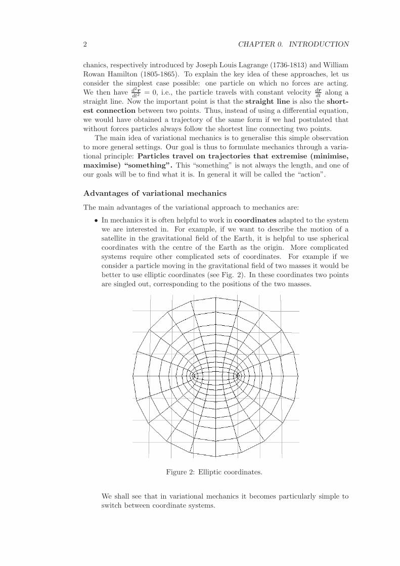
• In mechanics it is often helpful to work in coordinates adapted to the systemwe are interested in. For example, if we want to describe the motion of asatellite in the gravitational field of the Earth, it is helpful to use sphericalcoordinates with the centre of the Earth as the origin. More complicatedsystems require other complicated sets of coordinates. For example if weconsider a particle moving in the gravitational field of two masses it would bebetter to use elliptic coordinates (see Fig. 2). In these coordinates two pointsare singled out, corresponding to the positions of the two masses.
Figure 2: Elliptic coordinates.
We shall see that in variational mechanics it becomes particularly simple toswitch between coordinate systems.
3
• Many mechanical systems have constraints, i.e., conditions where particles orbodies are allowed to be and where not. A practical example would be a trainthat is required to stay on the railroad track. In variational mechanics theseconstraints can easily be incorporated by choosing appropriate coordinates,e.g., by taking the railroad track as a coordinate line.
• Crucially, many areas of mathematical physics are formulated in the lan-guage developped in variational mechanics. For instance “Hamiltonians” and“Lagrangians” play an important role in quantum mechanics or chaos the-ory. Similarly the ideas underlying variational mechanics are important in thetheory of differential equations.
(Rough) outline of this course
In this course, we will first develop the mathematical tools needed for extremisationproblems like the one sketched above (variational calculus). We will then considerboth the Lagrangian and the Hamiltonian formulation of mechanics and severalexamples for their use.
Reminder: Chain rule
As a preparation for many calculations in this course I want to remind how deriva-tives of expressions like
f(u(t), v(t), t)
are evaluated. According to the chain rule, we first have to differentiate w.r.t. thearguments of f , and then multiply with the derivatives of these arguments w.r.t. t.This yields
d
dtf(u(t), v(t), t) =
∂f
∂u(u(t), v(t), t)
du
dt+
∂f
∂v(u(t), v(t), t)
dv
dt+
∂f
∂t(u(t), v(t), t) .
Dropping the arguments and setting u = dudt , v = dv
dt , we can also write
df
dt=
∂f
∂uu +
∂f
∂vv +
∂f
∂t.
It is important to distinguish between the partial derivative ∂f∂t with respect to
the third argument of f , and the total derivative ∂f∂t where also the t-dependence
of the first and the second argument are taken into account.An example would be f representing the termperature felt by a person, f de-
noting the time, and u(t), v(t) the position of the person. Then the rate of changedfdt of the temperature felt will depend on the change of temperature with time (∂f
∂t )and on whether the person moves to a warmer or colder place (leading to the terms∂f∂u u and ∂f
∂v v).
4 CHAPTER 0. INTRODUCTION
Chapter 1
The calculus of variations
1.1 Example
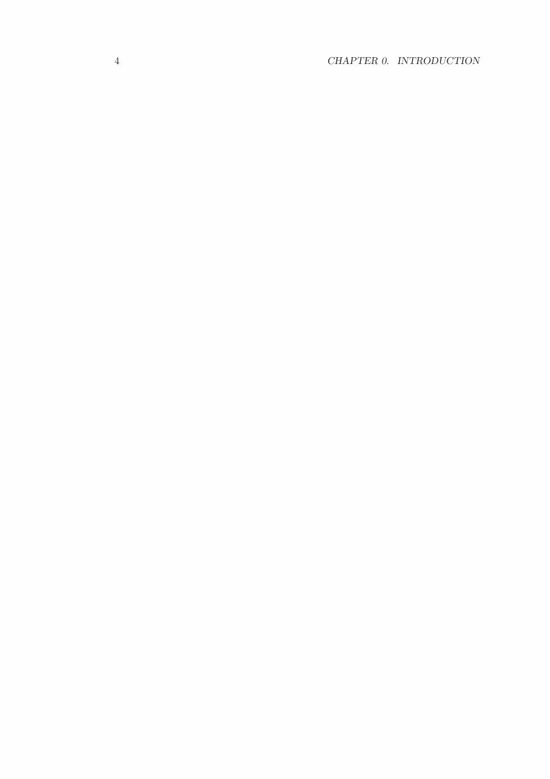
Figure 1.1: Possible connections between (x1, y1) and (x2, y2).
To introduce variational mechanics, we first need to equip ourselves with thetools needed to solve extremisation problems. We will start with the simplest ex-ample: Showing that the shortest connection between two points in R
2 is astraight line. Let us denote these two points by coordinates (x1, y1) and (x2, y2) ina Cartesian coordinate system, see Fig. 1.1. Curves connecting these two points canthen be described through functions y(x) that assign to each x-coordinate betweenx1 and x2 the corresponding y-coordinate. We now have to
• determine the length l of the curve corresponding to each function y(x)
• and find a y(x) such that l becomes minimal.
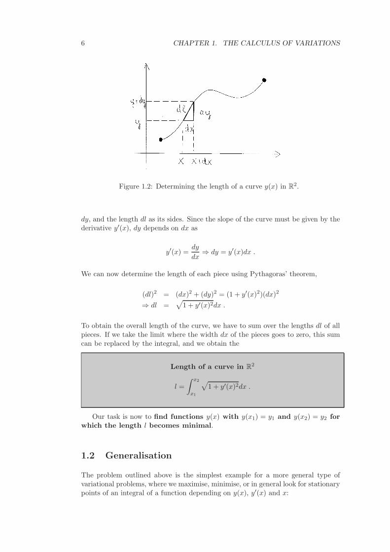
To start with the first task, we split the x-axis into small pieces of length dx.As seen in Fig. 1.2, this means that the curve is also split into small pieces, whoselength will be denoted by dl. We assume that the pieces are small enough such thatinside each piece the curve can be considered as a straight line. This means thatfor each piece we can draw a triangle as in Fig. 1.2 with the width dx, the height
5
6 CHAPTER 1. THE CALCULUS OF VARIATIONS
Figure 1.2: Determining the length of a curve y(x) in R2.
dy, and the length dl as its sides. Since the slope of the curve must be given by thederivative y′(x), dy depends on dx as
y′(x) =dy
dx⇒ dy = y′(x)dx .
We can now determine the length of each piece using Pythagoras’ theorem,
(dl)2 = (dx)2 + (dy)2 = (1 + y′(x)2)(dx)2
⇒ dl =√
1 + y′(x)2dx .
To obtain the overall length of the curve, we have to sum over the lengths dl of allpieces. If we take the limit where the width dx of the pieces goes to zero, this sumcan be replaced by the integral, and we obtain the
Length of a curve in R2
l =
∫ x2
x1
√
1 + y′(x)2dx .
Our task is now to find functions y(x) with y(x1) = y1 and y(x2) = y2 forwhich the length l becomes minimal.
1.2 Generalisation
The problem outlined above is the simplest example for a more general type ofvariational problems, where we maximise, minimise, or in general look for stationarypoints of an integral of a function depending on y(x), y′(x) and x:
1.2. GENERALISATION 7
Stationarity problem
Let
K[y] =
∫ x2
x1
f(y(x), y′(x), x)dx . (1.1)
Find y(x) satisfying the boundary conditions y(x1) = y1, y(x2) = y2 for whichK[y] becomes stationary.
The stationarity problem considered here are is different from those in Calculus,where the quantity to be minimised depended only on a single number or on avector. In contrast K[y] depends on a function. The mapping from y to K[y] isan example of a functional. A functional is a function that maps functions toreal numbers. Not all functionals are of the from in Eq. (1.1) (e.g. we mightalso have integrals depending on y′′(x)), but those of the type in Eq. (1.1) play aparticularly important role in mechanics. Another example for such a K[y] wouldbe K[y] =
∫ x2
x1(y(x)2 + y′(x)2)e−xdx.
To proceed, we have to understand better what it means for a functional to bestationary. We will define stationarity of functionals in terms of a stationarityproblem we are already familiar with: finding stationary points of a function thatonly depends on one variable. As a preparation let us consider a function y∗(x)satisfying our boundary conditions y∗(x1) = y1, y∗(x2) = y2 and then look atfunctions of the type
y∗(x) + ah(x) .
Here a is a real number, and h(x) is an abitrary but fixed function that satisfies theboundary conditions h(x1) = h(x2) = 0. The functions y∗(x)+ah(x) then satisfy thesame boundary conditions as y∗(x), i.e., y∗(x1)+ah(x1) = y1, y∗(x2)+ah(x2) = y2.We can evaluate the functional K with these functions as parameters, and get
K[y∗ + ah] =
∫ x2
x1
f(y∗(x) + ah(x), y′∗(x) + ah′(x), x)dx (1.2)
which is just a real number. We can now consider the values of K[y∗+ah] we get fordifferent a, and look for which values of a our K[y∗ + ah] becomes stationary. Thisis the type of stationarity problem we are know from calculus. K[y∗ + ah] becomesstationary for all a with
d
daK[y∗ + ah] = 0 . (1.3)
Now the point a = 0 corresponds to the function y∗, since for a = 0 we havey∗ + ah = y∗. For K to be stationary at y∗ we thus have to demand that (1.3)holds for a = 0. Since h was arbitrary, we have to demand this for all admissiblefunctions h. We thus obtain the following definition of stationarity for functionals:
K is stationary at a function y∗ if
d
daK[y∗ + ah]|a=0 = 0 (1.4)
holds for all functions h(x) with h(x1) = h(x2) = 0.
8 CHAPTER 1. THE CALCULUS OF VARIATIONS
1.3 Euler-Lagrange equation
We now want to derive a differential equation that can be used to find functionsy∗(x) for which K becomes stationary. To do so, let us assume that the functiony∗(x) is such a stationary point, and that it is also differentiable and satisfies ourboundary conditions.
First step: Use (1.4)
If we use (1.2) and the chain rule, Eq. (1.4) turns into
0 =d
daK[y∗ + ah]|a=0
=
∫ x2
x1
d
daf(y∗ + ah, y′∗ + ah′, x)
a=0
dx
=
∫ x2
x1
∂f
∂y(y∗ + ah, y′∗ + ah′, x)h(x) +
∂f
∂y′(y∗ + ah, y′∗ + ah′, x)h′(x)
a=0
dx .
We thus obtain
0 =
∫ x2
x1
∂f
∂y(y∗(x), y′∗(x), x)h(x) +
∂f
∂y′(y∗(x), y′∗(x), x)h′(x)
dx (1.5)
which needs to hold for all h(x) vanishing at x1 and x2. (At this point, it is alsoconvenient to drop the stars of y∗.)
Second step: Integrate by parts
We would like to simplify (1.5) such that both summands become proportional toh(x). This is easily achieved if we take the second summand and integrate by parts,
∫ x2
x1
∂f
∂y′︸︷︷︸
u
h′︸︷︷︸
v′
dx
=∂f
∂y′h∣∣x2
x1−∫ x2
x1
d
dx
(∂f
∂y′
)
h dx
= −∫ x2
x1
d
dx
(∂f
∂y′
)
h dx .
Here the term ∂f∂y′h
∣∣x2
x1could be dropped due to the boundary condition h(x1) =
h(x2) = 0. Inserting this result into (1.5) we obtain
∫ x2
x1
(∂f
∂y− d
dx
(∂f
∂y′
))
h(x) = 0 (1.6)
for arbitrary h(x).
Third step: Fundamental lemma of variational calculus
Obviously, Eq. (1.6) is satisfied if the term in brackets vanishes. Indeed the funda-mental lemma of variational calculus guarantees that this is the only way to satisfythe equation.
1.3. EULER-LAGRANGE EQUATION 9
Fundamental lemma of variational calculus
Suppose that g(x) is continuous, and
∫ x2
x1
g(x)h(x) = 0 (1.7)
holds for all h(x) satisfying h(x1) = h(x2) = 0. Then g(x) = 0 for all x ∈ (x1, x2).
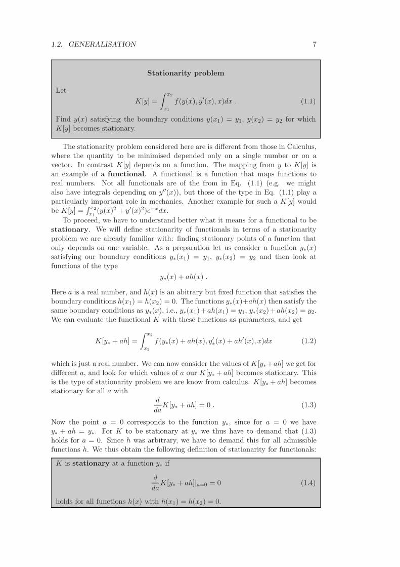
Proof: The proof proceeds by contradiction. Suppose that Eq. (1.7) holds forall h(x) and that we nevertheless have g(b) 6= 0 for one b ∈ (x1, x2), say, g(b) > 0(see Fig. 1.3). Due to the continuity of g(x) this implies that we have g(x) > 0in an interval around b. We now pick h(x) such that h(x) > 0 in this interval andh(x) = 0 outside. Then the integrand in Eq. (1.7) is positive in our interval and zerooutside, and the integral must be positive as well. This contradicts our assumption.Hence the theorem is proven.
Figure 1.3: The continuous function g(x) is positive in an interval around b.
The fundamental lemma of variational calculus implies that the term in bracketsin Eq. (1.6) vanishes. We thus see that functions extremising K =
∫ x2
x1f(y(x), y′(x), x)dx
have to satisfy the
Euler-Lagrange equation
∂f
∂y− d
dx
(∂f
∂y′
)
= 0
If we compare the Euler-Lagrange equation to the stationarity condition forfunctions of a single variable, it appears natural to identify the term of the left-hand side with a kind of derivative. Indeed,
δK
δy=
∂f
∂y− d
dx
∂f
∂y′
10 CHAPTER 1. THE CALCULUS OF VARIATIONS
is known as the functional derivative of K, and one can build a whole theory ofdifferentiation with respect to functions largely analogous to differentiationwith respect to numbers or vectors.1 This theory will not be considered further inthis lecture, since the Euler-Lagrange equation is already sufficient for our purposes.
1.4 Solution of our problem
The stationarity problem above was initially motivated by the search for curveswhere the length
l =
∫ x2
x1
(1 + y′(x)2)1/2dx
becomes minimal. We are now ready to solve this problem. The Euler-Lagrangeequation for f(y, y′, x) = (1 + y′2)1/2 reads
∂(1 + y′2)1/2
∂y− d
dx
∂(1 + y′2)1/2
∂y′= 0 .
The summand on the left-hand side vanishes since (1 + y′2)1/2 is independent of y.We thus find
d
dx
[
(1 + y′2)−1/2y′]
= 0
⇒ (1 + y′2)−1/2y′ = const
⇒ y′ = const .
The only curves with constant derivatives y′ are straight lines
y(x) = y′x + b .
The constants y′, b are now determined by the boundary conditions y(x1) = y1, y(x2) =y2. To incorporate y(x1) = y1 we set b = y1 − y′ · x1. This yields
y(x) = y′ · (x − x1) + y1
and indeed y(x1) = y1. The constant derivative y′ must then coincide with theslope of the straight line leading from (x1, y1) to (x2, y2)
y′ =y2 − y1
x2 − x1.
1.5 Alternative version of the Euler-Lagrange equation
If the integrand f in K does not depend explicitly on x the Euler-Lagrange equationcan be brought to a simpler form, also known as the Beltrami equation.
1See, e.g., Arfken, Mathematical Methods for Physicists or Gelfand and Fomin, Calculus of
Variations.
1.6. THE BRACHISTOCHRONE 11
Alternative version of the Euler-Lagrange equation
If f = f(y, y′) the Euler-Lagrange equation turns into
f − ∂f
∂y′y′ = const
(where ”const” means that f − ∂f∂y′ y′ does not depend on x).
Proof: Just use the chain rule to compute the total derivative of f − ∂f∂y′ y′ w.r.t.
x:d
dx
(
f − ∂f
∂y′y′)
=∂f
∂y
dy
dx+
∂f
∂y′dy′
dx−(
d
dx
∂f
∂y′
)
y′ − ∂f
∂y′dy′
dx
Here the second and the fourth summand cancel. If we use the Euler-Lagrangeequation d
dx∂f∂y′ = ∂f
∂y we see that also the first and third terms cancel, and we have
d
dx
(
f − ∂f
∂y′y′)
= 0 ,
as desired.Note: In contrast to the original Euler-Lagrange equation, this is a first-order
differential equation. It is typically much easier to use, since we can save the labourof taking derivatives w.r.t. y and x.
If we apply this formula our problem of finding the curve y(x) with minimallength l =
∫ x2
x1(1 + y′(x)2)1/2, we find
(1 + y′2)1/2 − (1 + y′2)−1/2y′2 = const ⇒ y′ = const
as before, i.e., we again see that the shortest connection between two points is astraight line.
1.6 The brachistochrone
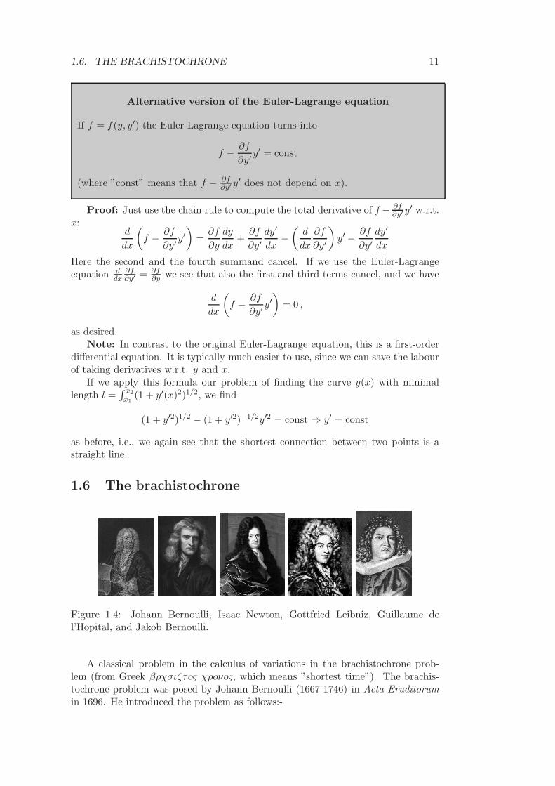
Figure 1.4: Johann Bernoulli, Isaac Newton, Gottfried Leibniz, Guillaume del’Hopital, and Jakob Bernoulli.
A classical problem in the calculus of variations in the brachistochrone prob-lem (from Greek βρχσιζτoς χρoνoς, which means ”shortest time”). The brachis-tochrone problem was posed by Johann Bernoulli (1667-1746) in Acta Eruditorum
in 1696. He introduced the problem as follows:-
12 CHAPTER 1. THE CALCULUS OF VARIATIONS
I, Johann Bernoulli, address the most brilliant mathematicians inthe world. Nothing is more attractive to intelligent people than an hon-est, challenging problem, whose possible solution will bestow fame andremain as a lasting monument. Following the example set by Pascal,Fermat, etc., I hope to gain the gratitude of the whole scientific commu-nity by placing before the finest mathematicians of our time a problemwhich will test their methods and the strength of their intellect. If some-one communicates to me the solution of the proposed problem, I shallpublicly declare him worthy of praise.
Solution were given by Isaac Newton (1643-1727), Gottfried Leibniz (1646-1716),Guillaume de l’Hopital (1661-1704) and Jakob Bernoulli (1654-1705, brother of theabove).
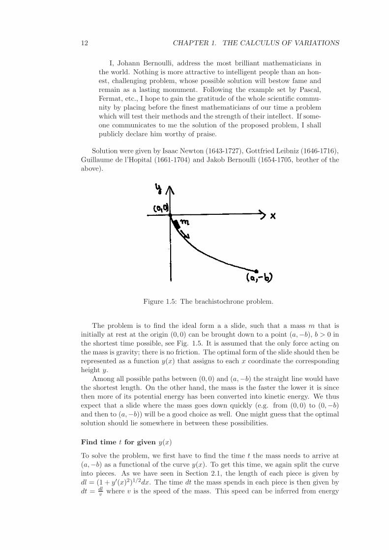
Figure 1.5: The brachistochrone problem.
The problem is to find the ideal form a a slide, such that a mass m that isinitially at rest at the origin (0, 0) can be brought down to a point (a,−b), b > 0 inthe shortest time possible, see Fig. 1.5. It is assumed that the only force acting onthe mass is gravity; there is no friction. The optimal form of the slide should then berepresented as a function y(x) that assigns to each x coordinate the correspondingheight y.
Among all possible paths between (0, 0) and (a,−b) the straight line would havethe shortest length. On the other hand, the mass is the faster the lower it is sincethen more of its potential energy has been converted into kinetic energy. We thusexpect that a slide where the mass goes down quickly (e.g. from (0, 0) to (0,−b)and then to (a,−b)) will be a good choice as well. One might guess that the optimalsolution should lie somewhere in between these possibilities.
Find time t for given y(x)
To solve the problem, we first have to find the time t the mass needs to arrive at(a,−b) as a functional of the curve y(x). To get this time, we again split the curveinto pieces. As we have seen in Section 2.1, the length of each piece is given bydl = (1 + y′(x)2)1/2dx. The time dt the mass spends in each piece is then given bydt = dl
v where v is the speed of the mass. This speed can be inferred from energy
1.6. THE BRACHISTOCHRONE 13
conservation. At the starting point (0, 0) the mass neither has potential nor kineticenergy. At a later point at height y < 0 the potential energy is mgy, and the kineticenergy has increased to m
2 v2. Energy conservation now implies that
E = 0 = mgy +1
2mv2
⇒ v = (−2gy)1/2 .
Using this result for the speed and the length dl calculated above we obtain thetime spend in each piece of the curve as
dt =dl
v=
(1 + y′(x)2
−2gy(x)
)1/2
.
If we integrate over dt we see that the travel time of the mass is given by
t =1
(2g)1/2
∫ a
0
(1 + y′(x)2
−y(x)
)1/2
︸ ︷︷ ︸
≡f
dx .
Find minima
We now have to find the curve y(x) for which t becomes minimal. To do so we usethe alternative version of the Euler-Lagrange equation
f − ∂f
∂y′y′ = const
If we insert the f given above, we obtain
(1 + y′2
−y
)1/2
−12 (1 + y′2)−1/22y′
(−y)1/2y′ = const
⇒ 1
(−y)1/2(1 + y′2)1/2= const
Thus the term (−y)(1 + y′2) in the denominator must be constant. If we denotethis constant by 2R we obtain
1 + y′2 =2R
−y
⇒ y′ = ∓(
2R + y
−y
)1/2
(1.8)
At least initially, the sign above must be negative since we would expect the massto fall down. We have thus obtained a differential equation giving the derivative y′
as a function of y.
Solving the differential equation
We solve the differential equation by separation. We thus write y′ = dydx ⇒ dy
y′ = dxand then integrate on both sides. In our case the integration limits have to be 0and a for x and y(0) = 0 and y(x) for y. We thus obtain
∫ y(x)
0
dy
y′=
∫ x
0dx = x
14 CHAPTER 1. THE CALCULUS OF VARIATIONS
and, inserting the formula for y′,
−∫ y(x)
0
( −y
2R + y
)1/2
dy = x . (1.9)
To proceed we need to evaluate the integral over y. This can be accomplished withthe trigonometric substitution
y = −2R sin2 θ
2(1.10)
Note that in the beginning of the curve we must have y = 0 and thus θ = 0.Differentiation now yields
dy = −2R sinθ
2cos
θ
2dθ
and the denominator in Eq. (1.9) simplifies to
(2R + y)1/2 = (2R(1 − sin2 θ
2))1/2 = (2R)1/2 cos
θ
2
If we substitute all these formulas into Eq. (1.9) we obtain
x = 2R
∫ θ(x)
0sin2 θ
2dθ = R
∫ θ(x)
0(1 − cos θ)dθ = R(θ(x) − sin θ(x)) . (1.11)
Result
One could attempt to solve (1.10) and (1.11) to get y in terms of x but it is easier torepresent the solution curve in parametrised form, leaving both x and y as functionsof θ. Indeed (1.10) and (1.11) boil down to
x(θ) = R(θ − sin θ)
y(θ) = −2R sin2 θ
2= −R(1 − cos θ) (1.12)
A plot of the resulting x(θ), y(θ) is shown in figure 1.6. We see that for θ =0, 2π, 4π, . . . the coordinate y reaches zero whereas x is equal to 0, 2πR, 4πR, . . .. Atthese points the curve has a cusp, and the slope becomes infinite on both sides ofthe cusp. At θ = π, 3π, 5π, . . . there are minima with y = −2R. Strictly speakingour results only apply up to the first minimum at θ = π since we only considered theregime where y decreases with increasing x and chose the sign in (1.8) accordingly.However by repeating our calculation with small modifications for other values ofθ, one can see that the solution obtained is actually valid for arbitary θ.
It is instructive to to write (1.12) in vector notation,(
x(θ)y(θ)
)
=
(0
−R
)
+
(R0
)
θ + R
(− sin θcos θ
)
(1.13)
Eq. (1.13) has the following interpretation: If we momentarily forget about the thirdterm on the right-hand side of (1.13), the vectors (x, y) would start from (0,−R) atθ = 0; as θ increases they would then move on a straight line in positive x-direction.In contrast, the third term describes a motion around a circle of radius R, i.e., arotation. We thus see that as θ increases the points (x, y) follow a superposition ofa motion on a straight line and a rotation.

1.6. THE BRACHISTOCHRONE 15
Figure 1.6: θ, x, and y for the brachistochrone problem.
A related problem
The same curve (1.13) but with opposite sign of y is obtained in a completelydifferent problem: the motion of a disk with radius R rolling over the x-axis. Thiscurve is called the cycloid curve.
To also get the sign as in (1.13) we instead compare with the more artificialsituation where a disk is “rolling” below the x-axis. If the disk is rolling into positivex direction, its centre point moves on a straight line with increasing x. A point (x, y)on the circumference of the disk follows that straight-line motion, but at the sametime rotates around the centre. If one observes a rolling disk, one can see that thepoint actually rotates to the left. This is in line with (1.13) since (− sin θ, cos θ) =(cos(
π2 + θ
), sin
(π2 + θ
))gives a rotation to the left if θ is increased. During one
revolution (i.e. an increase of θ by 2π) the disk should move by a distance thatcoincides with the circumference 2πR, i.e., x should increase by 2πR just as in(1.13).
Boundary conditions
We still have to find the right value for R. Moreover we must find out which partof Fig. 1.6 should be taken as our ideal slide; this part must certainly start at theorigin but we have to know at which value θend of θ it has to end. R and θend canbe found by inserting the boundary conditions x(θend) = a, y(θend) = −b into Eq.(1.13). We then obtain the nonlinear system of equations
a = R(θend − sin θend)
−b = −R(1 − cos θend)
which will be considered further on the second problem sheet.
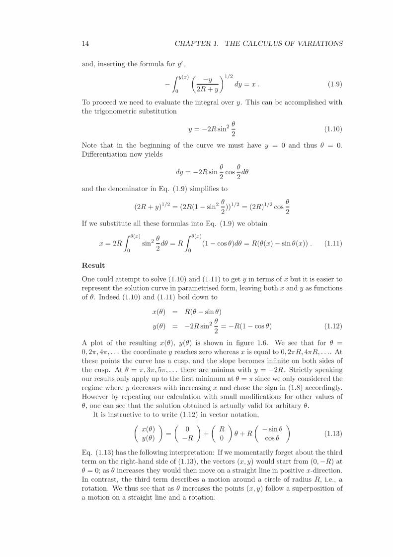
Qualitatively the most interesting question is whether the slide will end to theleft or to the right of the minimum at θ = π. In the first case the slide will alwaysgo down (see Fig. 1.6a) whereas in the second case it will first go down and thenup again (see Fig. 1.6b). If we compare the curve in Fig. 1.6 to the line y = −2x
π ,we see that to the left of the minimum the curve always satisfies y < −2x
π whereasto the right we have y > −2x
π inserting x(θend) = a, y(θend) = −b we thus see thatthe endpoint will be to the left if
−b < −2a
π⇔ 2a
b< π . (1.14)
16 CHAPTER 1. THE CALCULUS OF VARIATIONS
In this case the slide will always go down whereas otherwise it first goes down andthen up.
Figure 1.7: Solution of the brachistochrone problem: (a) for 2ab < π, (b) for 2a
b > π.
1.7 Functionals depending on several functions
So far we only considered variational problems that involved one function y(x) map-ping R to R. However one often encounters problems that involve several functionsof this type. Let us thus consider n different functions y1(x), y2(x), . . . , yn(x), eachsubject to boundary conditions at x1 and x2, and then define a functional dependingon all of them
K[y1, . . . , yn] =
∫ x2
x1
f(y1(x), . . . , yn(x), y′1(x), . . . , y′n(x), x)dx .
We want to find y1(x), y2(x), . . . , yn(x) such that K becomes stationary w.r.t. vari-ations of all n functions. K will be stationary w.r.t. variations of yj(x) if thecorresponding Euler-Lagrange equation
∂f
∂yj− d
dx
∂f
∂y′j= 0 (1.15)
is satisfied. To make K stationary w.r.t. variations of all function we thus have todemand that (1.15) holds for all j from 1 to n.
Note: It is often convenient to collect all functions yj(x) into a vector-valuedfunction y(x) = (y1(x), . . . , yn(x)).
1.8 Fermat’s principle
To illustrate the use of variational calculus in Rn we consider an example from
optics. (Geometric) optics can be based on a variational principle formulated byFermat:
Fermat’s principle
Light travels between two points on paths (rays) that take the least (or stationary)time.
These light rays are very similar to particle trajectories in mechanics. To make useof Fermat’s principle we have to recall that the speed of light is given by c
n where
1.8. FERMAT’S PRINCIPLE 17
c is the speed of light in vacuum and the refraction index n > 1 depends onthe medium in which the light is propagating. In many applications the refractionindex and thus the speed of light is constant. Then Fermat’s principle implies thatalso the length of the rays is stationary. Light thus moves on straight lines. (Itcan also be reflected by a mirror; as seen on a problem sheet rays where light isreflected from the mirror according to the reflection law ”angle of incidence = angleof reflection” have stationary length.)
We now want to consider the situation where the refraction index is notconstant, i.e., we have n = n(x, y, z).
Find t as functional of the path
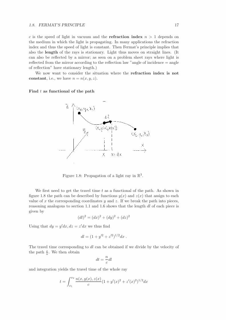
Figure 1.8: Propagation of a light ray in R3.
We first need to get the travel time t as a functional of the path. As shown infigure 1.8 the path can be described by functions y(x) and z(x) that assign to eachvalue of x the corresponding coordinates y and z. If we break the path into pieces,reasoning analogous to section 1.1 and 1.6 shows that the length dl of each piece isgiven by
(dl)2 = (dx)2 + (dy)2 + (dz)2
Using that dy = y′dx, dz = z′dx we thus find
dl = (1 + y′2 + z′2)1/2dx .
The travel time corresponding to dl can be obtained if we divide by the velocity ofthe path c
n . We then obtain
dt =n
cdl
and integration yields the travel time of the whole ray
t =
∫ x2
x1
n(x, y(x), z(x)
c(1 + y′(x)2 + z′(x)2)1/2dx
18 CHAPTER 1. THE CALCULUS OF VARIATIONS
Find stationary points of t
We now need to find y(x), z(x) such that the travel time t becomes extremal. Wethus face an extremisation problem of the type discussed in section 1.7, with theidentifications
K = t
(y1, y2) = (y, z)
f =n(x, y(x), z(x)
c(1 + y′(x)2 + z′(x)2)1/2
︸ ︷︷ ︸
=u(x)
To solve this extremisation problem we have to consider the Euler-Lagrangeequations for both y(x) and z(x). For y(x) we obtain
∂f
∂y− d
dx
∂f
∂y′= 0
⇒ 1
c
∂n
∂yu − d
dx
(n
c
1
2u−12y′
)
= 0
⇒ d
dx
(ny′
u
)
=∂n
∂yu (1.16)
For z(x) analogous reasoning yields
∂f
∂z− d
dx
∂f
∂z′= 0
⇒ d
dx
(nz′
u
)
=∂n
∂zu (1.17)
These equations must now be solved for y(x), z(x) to get rays.
Special case
Figure 1.9: A ray of light in two dimensions.
1.8. FERMAT’S PRINCIPLE 19
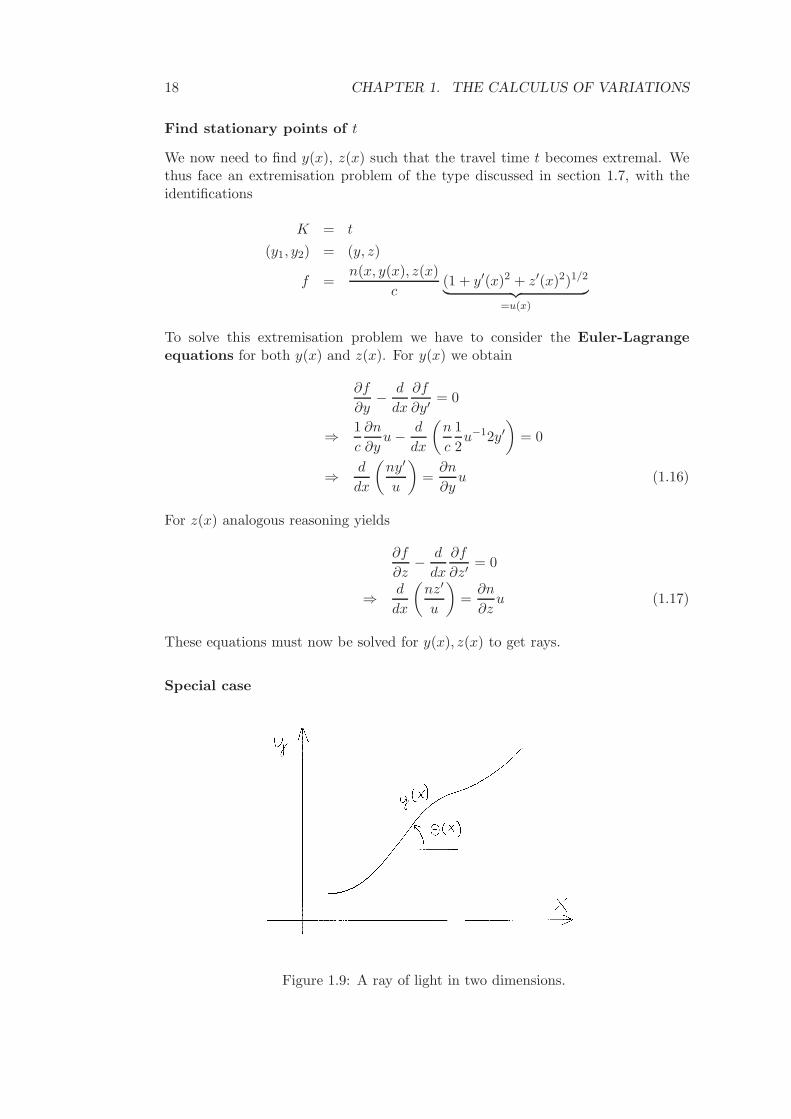
For definiteness, let us consider the special case where the refraction indexdepends only on x, i.e. n = n(x) and ∂n
∂y = ∂n∂z = 0. Then the Euler-Lagrange
equations (1.16) and (1.17) boil down to
ny′
u= const
nz′
u= const (1.18)
Let us moreover assume that the z-coordinate is always zero, a condition that iscertainly in line with (1.18). In this case the light rays only travel in the x−y-plane,see figure 1.9. If we insert the definition of u the second equation in (1.18) thenboils down to
ny′
(1 + y′2)1/2= const (1.19)
Eq. (1.19) can be simplified if we express the slope y′(x) of the curve in Fig. 1.9through the angle θ(x) enclosed between the curve and the x-direction. We thenwrite
y′(x) = tan θ(x)
and simplify the denominator in (1.19),
(1 + y′(x)2)1/2 = (1 + tan2 θ(x))1/2 =
(cos2 θ(x) + sin2 θ(x)
cos2 θ(x)
)1/2
=1
cos θ(x).
Eq. (1.19) thus turns into
n(x) sin θ(x) = const
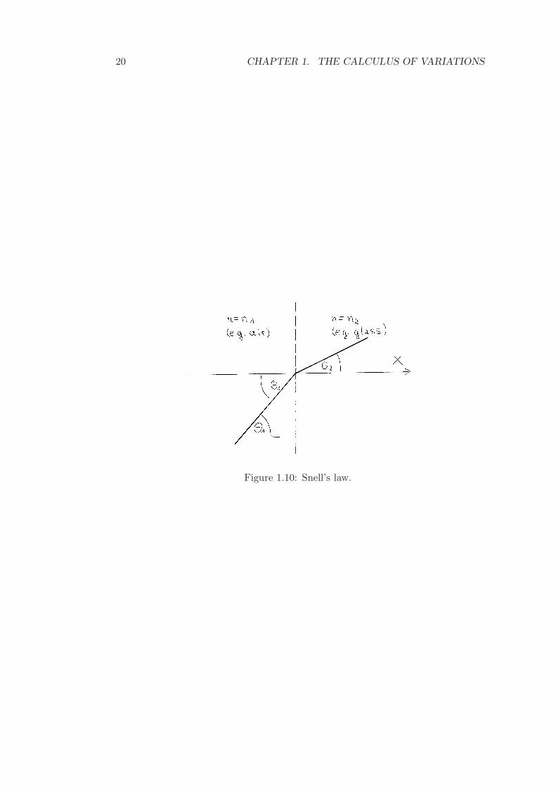
which is known as (the generalised version of) Snell’s law.For example, let us assume that the space x < 0 is filled with a medium with
constant refraction index n = n1 (say, air) and the space x > 0 is filled with adifferent medium with n = n2 (say, glass), see Fig. 1.10. Inside both media therays travel on straight lines enclosing angles θ1 and θ2 with the x-direction. Givenθ1 the angle θ2 is then determined by
n1 sin θ1 = n2 sin θ2
This equation is the original formulation of Snell’s law.
20 CHAPTER 1. THE CALCULUS OF VARIATIONS
Figure 1.10: Snell’s law.
Chapter 2
Lagrangian mechanics
2.1 Reminder: Newton
We now want to formulate mechanics through a variational principle. As a prepa-ration, we need to review some basic facts from Newtonian mechanics. We considersystems of N particles with masses m1,m2, . . . ,mN at positions r1, r2, . . . rN . Eachof these positions is a vector ri = (xi, yi, zi) ∈ R
3.
The particle trajectories ri(t) are now determined by Newton’s second law
miri(t) = F i(r1(t), . . . , rN (t), r1(t), . . . , rN (t))
where F i is the force acting on the i-th particle. A particularly important type offorces are conservative forces: Forces are conservative if they can be written asderivatives of a potential energy U ,
F i = − ∂
∂riU(r1, . . . , rN ) .
Here ∂U∂ri
is the gradient
∂U/∂xi
∂U/∂yi
∂U/∂zi
.
Example: In a uniform gravity field (e.g. the gravity field of the earth in thevicinity of the surface of the earth) a particle at r = (x, y, z) has the potential
U = mgz ,
and thus feels the force
F = −
∂U/∂x∂U/∂y∂U/∂z
=
00
−mg
Finally, our system of N particles has the kinetic energy
T =
N∑
i=1
1
2mir
2i .
21
22 CHAPTER 2. LAGRANGIAN MECHANICS
2.2 Lagrangian mechanics in Cartesian coordinates
In Lagrangian mechanics, the laws of motion are formulated in terms of variationalcalculus, i.e., by demanding that a certain functional should become stationary.This approach has several advantages over direct use of Newtonian mechanics thatwill become clear over the course of this lecture. We will first develop the variationalformulation for the simplest case, assuming that all forces are conservative and allparticle coordinates are indicated in Cartesian coordinates.
The functions to be determined in mechanics are the particle trajectories ri(t).We thus need a variational principle that tells us how particles move from given
positions ri(t(1)) = r
(1)i at time t(1) to given positions ri(t
(2)) = r(2)i at time t(2).
In our variational principle the role of the integrand f will be played by thedifference of the kinetic and potential energy, the so-called Lagrangian
L(r1, . . . , rN , r1, . . . , rN ) = T (r1, . . . , rN ) − U(r1, . . . , rN )
The Lagrangian depends both on the particle positions (determining U) and the ve-locities (determining T ).
We then define a functional called the action S, by taking the time integral ofthe Lagrangian from t(1) to t(2):
S[r1, . . . , rN ] =
∫ t(2)
t(1)L(r1(t), . . . , rN (t), r1(t), . . . , rN (t))dt .
Now the claim is that the particles travel on trajectories ri(t) for which S be-comes stationary. For historical reasons this famous principle (due to Hamilton andMaupertius) is known as the principle of least action (rather than stationary action,which would be the correct terminology).
Principle of “least” action
In a systen where all forces are conservative the trajectories of particles moving
from positions ri(t(1)) = r
(1)i to positions ri(t
(2)) = r(2)i are chosen such that
the action becomes stationary w.r.t. variations that preserve these boundaryconditions, i.e., the Euler-Lagrange equations
∂L
∂ri=
d
dt
∂L
∂ri(2.1)
must be satisfied, for all i = 1 . . . N .
Here the vector equation (2.1) implies that the coordinates xi of the i-th particlemust satisfy ∂L
∂xi= d
dt∂L∂xi
, and analogous equations hold for yi and zi. Altogether wethus obtain 3N equations for N particles described by 3 coordinates each. In thecontext of Lagrangian mechanics the Euler-Lagrange equations are usually calledLagrange’s equations.
Note: When comparing to the section 1, we have to identify K = S, x = t and(y1(x), . . . , yn(x)) = (r1(t), . . . , rN (t)).
Proof: The principle of least action is equivalent to Newton’s second law. Ifall forces are conservative this can be shown in a surprisingly simple way. The
2.2. LAGRANGIAN MECHANICS IN CARTESIAN COORDINATES 23
derivative ∂L∂ri
in the Lagrange equation can be written as
∂L
∂ri= −∂U
∂ri= F i
where we used that the Lagrangian depends on the particle coordinates ri onlythrough the potential and that derivatives of the potential yield forces. On theother hand, the Lagrangian depends on the velocities ri only through the kineticenergy. We thus obtain
∂L
∂ri=
∂T
∂ri= miri
⇒ d
dt
∂L
∂ri= miri .
By inserting these result into Eq. (2.1) we see that the Lagrange equations areequivalent to
F i = miri,
i.e., Newton’s second law.
Examples:
• If there is no potential and just a single particle we have L = T = 12mr2 and
S =∫ t(2)
t(1)12mr2(t)dt and the Lagrange equation reads
∂L
∂r=
d
dt
∂L
∂r⇒ 0 =
d
dtmr ⇒ r = const,
i.e., the particle is moving on a straight line with constant velocity. (Notethat if we would just demand that the length becomes stationary, we wouldget slightly less: we would only see that there is a straight line, but not thatthis line is traversed with constant velocity.)
• A particle at r = (x, y, z) in a uniform gravity field has the Lagrangian
L = T − U =1
2m(x2 + y2 + z2) − mgz
The Lagrange equations for x, y and z read
∂L
∂x=
d
dt
∂L
∂x⇒ 0 =
d
dtmx ⇒ x = const
∂L
∂y=
d
dt
∂L
∂y⇒ 0 =
d
dtmy ⇒ y = const
∂L
∂z=
d
dt
∂L
∂z⇒ −mg =
d
dtmz ⇒ z = −g
As expected, we get an acceleration g in negative x-direction.
24 CHAPTER 2. LAGRANGIAN MECHANICS
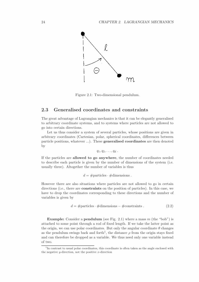
Figure 2.1: Two-dimensional pendulum.
2.3 Generalised coordinates and constraints
The great advantage of Lagrangian mechanics is that it can be elegantly generalisedto arbitrary coordinate systems, and to systems where particles are not allowed togo into certain directions.
Let us thus consider a system of several particles, whose positions are given inarbitrary coordinates (Cartesian, polar, spherical coordinates, differences betweenparticle positions, whatever ...). These generalised coordinates are then denotedby
q1, q2, . . . , qd .
If the particles are allowed to go anywhere, the number of coordinates neededto describe each particle is given by the number of dimensions of the system (i.e.usually three). Altogether the number of variables is thus
d = #particles · #dimensions .
However there are also situations where particles are not allowed to go in certaindirections (i.e., there are constraints on the position of particles). In this case, wehave to drop the coordinates corresponding to these directions and the number ofvariables is given by
d = #particles · #dimensions − #constraints . (2.2)
Example: Consider a pendulum (see Fig. 2.1) where a mass m (the “bob”) isattached to some point through a rod of fixed length. If we take the latter point asthe origin, we can use polar coordinates. But only the angular coordinate θ changesas the pendulum swings back and forth1, the distance ρ from the origin stays fixedand can therefore be dropped as a variable. We thus need only one variable insteadof two.
1In contrast to usual polar coordinates, this coordinate is often taken as the angle enclosed withthe negative y-direction, not the positive x-direction
2.3. GENERALISED COORDINATES AND CONSTRAINTS 25
We will see several more complicated examples of such constraints later in thelecture. The space of all allowed positions of particles parametrised by the co-ordinates q1, q2, . . . qd is called the configuration space of the system. Thesecoordinates are also called the degrees of freedom of the system.
Relation between generalised and Cartesian coordinates
The generalised coordinates determine the Cartesian particle positions ri, i.e., wecan write ri as a function of q1, . . . , qd. Being slightly more general, we could couldallow for ri to depend on times as well, and write
ri = ri(q1, . . . , qd, t) . (2.3)
(This includes the case that e.g. the origin of our generalised coordinate systemmoves in time – a situation that won’t occur often in this course.) Given Eq. (2.3),the particle velocities ri can be determined using the chain rule,
ri =dri
dt=
d∑
α=1
∂ri
∂qαqα +
∂ri
∂t. (2.4)
Here the right-hand side involves generalised coordinates, their derivatives and time.Hence we can express ri as a function of q1, . . . , qd, q1, . . . qd and t.
Lagrangian mechanics
We can now use these relations to express all quantities relevant for Lagrangianmechanics in terms of the new coordinates. Using (2.3) we can write the potentialenergy as a function
U = U(q1, . . . , qd, t) .
Expressing the velocities through (2.4) we can write the kinetic energy as a function
T = (q1, . . . , qd, q1, . . . , qd, t) .
The Lagrangian thus turns into a function
L(q1, . . . , qd, q1, . . . , qd, t) = T (q1, . . . , qd, q1, . . . , qd, t) − U(q1, . . . , qd, t) ,
and the action can be written as a functional depending on the functions q1(t), . . . , qd(t),
S[q1, . . . , qd] =
∫ (2)
t(1)L(q1(t), . . . , qd(t), q1(t), . . . , qd(t), t)dt .
The boundary conditions can be expressed as
qα(t(1)) = q(1)α , qα(t(2)) = q(2)
α .
We now claim that a result analogous to Eq. (2.1) also holds for q1, . . . , qd.This means that (i) the Lagrangian formulation of mechanics holds is valid forarbitrary coordinate systems and (ii) that it also holds for systems with constraints.The second point applies even though the forces that give rise to these constraints(e.g. the tension force preventing us from increasing the length of a pendulum) aretypically non-conservative!
26 CHAPTER 2. LAGRANGIAN MECHANICS
Principle of “least” action (general form)
Consider systems where all forces are either conservative or give rise to con-straints. For such systems all qα(t) are chosen such that the action S becomesstationary w.r.t. variations of qα(t) that preserve the boundary conditions at t(1)
and t(2). We thus have∂L
∂qα=
d
dt
∂L
∂qα
for all α = 1 . . . d.
The proof of this statement will be given later, after discussing some examples.(The tricky bit will be the generalisation to systems with constraints. If not for theconstraints, we could give a very short proof. Essentially, we could invoke the prooffor Cartesian coordinates and then argue that an extremum of the action remainsan extremum of the action regardless of which system of coordinates we are workingin.)
2.3.1 Gravitational field
As a first example for Lagrangian mechanics with generalised coordinates let usconsider the trajectory r(t) of a mass m (e.g. the earth) in the gravitational fieldof a mass M (e.g. the sun) at the origin. The corresponding gravitational potentialreads U = −GmM
|r| and the kinetic energy is, of course, given by T = 12mr2.
The symmetry of the problem now suggests to work in spherical coordinates,where the vectors r are parametrised by their distance from the origin ρ and twoangles θ and φ:
r = ρ
sin θ cos φsin θ sin φ
cos θ
In spherical coordinates the potential energy U turns into
U = −GmM
ρ.
To get the kinetic energy, we use that
r = ρ
sin θ cos φsin θ sinφ
cos θ
+ ρθ
cos θ cos φcos θ sin φ− sin θ
+ ρφ sin θ
− sin φcos θ
0
where the three vectors multiplied with ρ, ρθ and ρφ sin θ are all normalised andperpendicular to each other. We thus get
T =m
2r2 =
m
2(ρ2 + ρ2θ2 + ρ2φ2 sin2 θ)
Note that in contrast to the Cartesian case T does not only depend on the derivativesρ, θ, φ but also on ρ and θ. The Lagrangian can now be written as
L(ρ, θ, φ, ρ, θ, φ) = T − U =m
2(ρ2 + ρ2θ2 + ρ2φ2 sin2 θ) +
GmM
ρ
2.3. GENERALISED COORDINATES AND CONSTRAINTS 27
and the action S can be written as a functional of ρ(t), θ(t), and φ(t):
S =
∫ t(2)
t(1)L(ρ(t), θ(t), φ(t), ρ(t), θ(t), φ(t))dt . (2.5)
The principle of stationary action now gives rise to Lagrange equations for ρ, θand φ:
∂L
∂ρ=
d
dt
∂L
∂ρ⇒ mρθ2 + mρ sin2 θφ2 − GmM
ρ2= mρ
∂L
∂θ=
d
dt
∂L
∂θ⇒ mρ2 sin θ cos θφ2 =
d
dt(mρ2θ)
∂L
∂φ=
d
dt
∂L
∂φ⇒ 0 =
d
dt(mρ2φ sin2 θ)
We thus see that Lagrange’s formulation of mechanics makes it simple to switchbetween coordinate systems: One only has to rewrite the Lagrangian in terms ofthe new coordinates and invoke Lagrange’s equations which have the same form inevery coordinate system.
2.3.2 Pendulum
To illustrate Lagrangian mechanics for systems with constraints, let us consider theexample of the pendulum. The generalised coordinate −π < θ < π depicted in Fig.2.1 determines the x- and y-coordinates of the mass m as
x = l sin θ
y = −l cos θ .
The derivatives of these coordinates read
x = l cos θ θ
y = l sin θ θ
and determine the kinetic energy as
T =1
2m(x2 + y2) =
1
2ml2θ2
The potential energy is simply given by
U = mgy = −mgl cos θ
The Lagrangian thus takes the form
L = T − U =1
2ml2θ2 + mgl cos θ .
The Lagrange equation for our generalised coordinate θ now reads
∂L
∂θ=
d
dt
∂L
∂θ.
28 CHAPTER 2. LAGRANGIAN MECHANICS
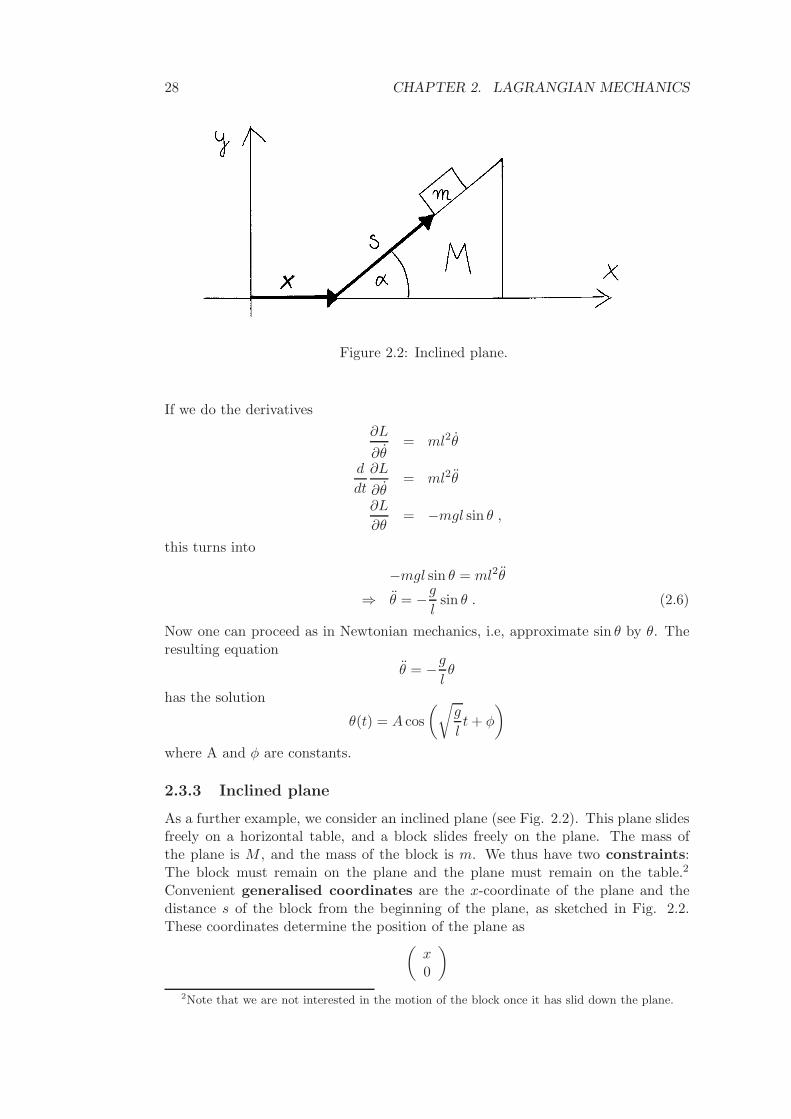
Figure 2.2: Inclined plane.
If we do the derivatives
∂L
∂θ= ml2θ
d
dt
∂L
∂θ= ml2θ
∂L
∂θ= −mgl sin θ ,
this turns into
−mgl sin θ = ml2θ
⇒ θ = −g
lsin θ . (2.6)
Now one can proceed as in Newtonian mechanics, i.e, approximate sin θ by θ. Theresulting equation
θ = −g
lθ
has the solution
θ(t) = A cos
(√g
lt + φ
)
where A and φ are constants.
2.3.3 Inclined plane
As a further example, we consider an inclined plane (see Fig. 2.2). This plane slidesfreely on a horizontal table, and a block slides freely on the plane. The mass ofthe plane is M , and the mass of the block is m. We thus have two constraints:The block must remain on the plane and the plane must remain on the table.2
Convenient generalised coordinates are the x-coordinate of the plane and thedistance s of the block from the beginning of the plane, as sketched in Fig. 2.2.These coordinates determine the position of the plane as
(x0
)
2Note that we are not interested in the motion of the block once it has slid down the plane.
2.3. GENERALISED COORDINATES AND CONSTRAINTS 29
and the position of the block as
r =
(x + s cos α
s sinα
)
The kinetic energy of the plane reads 12Mx2, whereas the block has the kinetic
energy 12mr2. To express 1
2mr2 in terms of our generalised coordinates we write
r =
(x + s cos α
s sin α
)
r2 = (x + s cos α)2 + (s sin α)2 = x2 + s2 + 2xs cos α .
The overall kinetic energy is thus obtained as
T =1
2Mx2 +
1
2m(x2 + s2 + 2xs cos α) =
1
2(M + m)x2 +
1
2ms2 + mxs cos α .
The only contribution to the potential energy U is due to the height of the block,
U = mgs sin α .
The Lagrangian thus reads
L = T − U =1
2(M + m)x2 +
1
2ms2 + mxs cos α − mgs sin α .
We now obtain two Lagrange equations, one for the coordinate x and one for s.For x we get
∂L
∂x− d
dt
∂L
∂x= 0 .
With the derivatives
∂L
∂x= (M + m)x + m cos αs
d
dt
∂L
∂x= (M + m)x + m cos αs
∂L
∂x= 0
this turns into
−(M + m)x − m cos αs = 0 . (2.7)
The Lagrange equation for s reads
∂L
∂s− d
dt
∂L
∂s= 0 .
If we use the derivatives
∂L
∂s= ms + m cos αx
d
dt
∂L
∂s= ms + m cos αx
∂L
∂s= −mg sin α
30 CHAPTER 2. LAGRANGIAN MECHANICS
and cancel the factors −m this simplifies to
s + cos αx + g sin α = 0 . (2.8)
We have thus obtained two coupled equations (2.7), (2.8) for the second derivativesx and s. To obtain separate equations for x and s, we solve (2.7) for x and use itto eliminate x in (2.8). This yields
s − m
M + mcos2 αs + g sin α = 0
⇒ (M + m)s − m cos2 αs + (M + m)g sin α = 0
⇒ (M + m sin2 α)s + (M + m)g sinα = 0
which finally leads to
s = −(M + m)g sin α
M + m sin2 α= const . (2.9)
If we substitute (2.9) back into (2.7) we get
x =mg
M + m sin2 αsin α cos α = const. (2.10)
Eq. (2.9) and (2.10) give the second derivatives of our generalised coordinates asconstants depending on the parameters of the problem. One easily checks that inspecial cases like α → 0, α → π
2 or m → 0 these results agree with what we mightexpect. (E.g. for a perpendicular plane with α = π
2 the block simply falls downwith s = −g whereas the plane stays fixed.) Assuming that the block and the planeare initially at rest we can integrate (2.9) and (2.10), to get
x(t) = x(0) +1
2xt2
s(t) = s(0) +1
2st2 .
For comparison: Inclined plane with Newton
It is instructive to compare the above treatment of the inclined plane with New-tonian mechanics. The main difference will be that in Newtonian mechanics theconstraints can no longer be built in by choosing appropriate generalised coordi-nates. Instead one has to work in Cartesian coordinates and take into account allforces acting on the plane and the block; in particular this includes forces that makesure that the constraints are satisfied.
Forces acting on the inclined plane
For the inclined plane Newton’s law implies
F P = MaP
where
aP =
(x0
)
is the acceleration of the plane and F P is the sum of all forces acting on the plane(see Fig. 2.3):
2.3. GENERALISED COORDINATES AND CONSTRAINTS 31
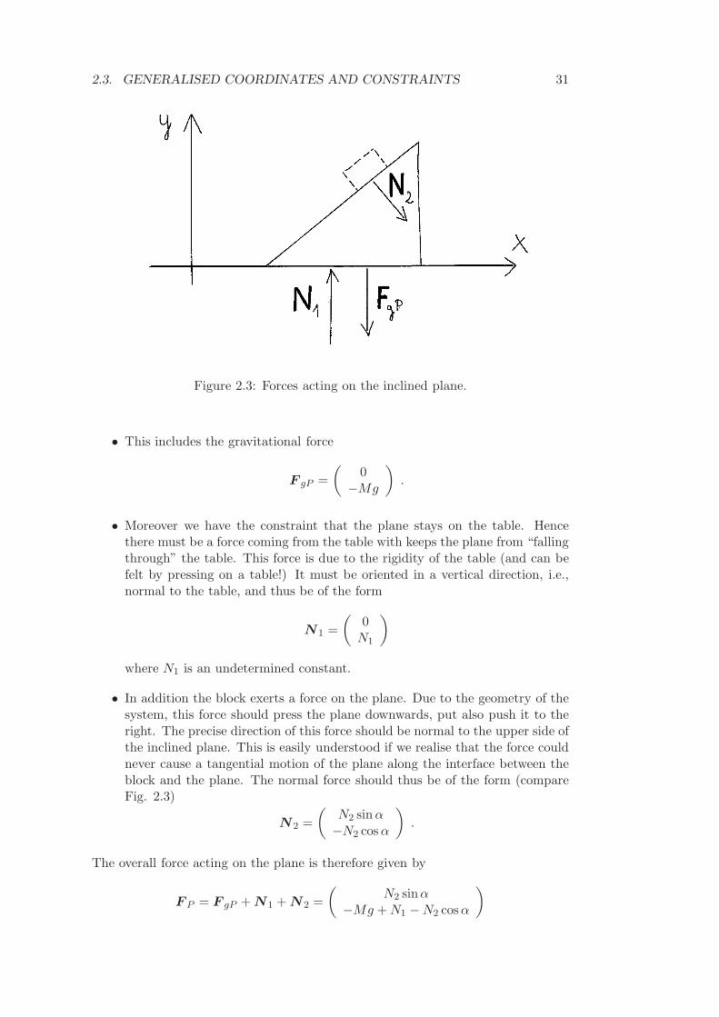
Figure 2.3: Forces acting on the inclined plane.
• This includes the gravitational force
F gP =
(0
−Mg
)
.
• Moreover we have the constraint that the plane stays on the table. Hencethere must be a force coming from the table with keeps the plane from “fallingthrough” the table. This force is due to the rigidity of the table (and can befelt by pressing on a table!) It must be oriented in a vertical direction, i.e.,normal to the table, and thus be of the form
N 1 =
(0
N1
)
where N1 is an undetermined constant.
• In addition the block exerts a force on the plane. Due to the geometry of thesystem, this force should press the plane downwards, put also push it to theright. The precise direction of this force should be normal to the upper side ofthe inclined plane. This is easily understood if we realise that the force couldnever cause a tangential motion of the plane along the interface between theblock and the plane. The normal force should thus be of the form (compareFig. 2.3)
N 2 =
(N2 sin α−N2 cos α
)
.
The overall force acting on the plane is therefore given by
F P = F gP + N1 + N 2 =
(N2 sinα
−Mg + N1 − N2 cos α
)
32 CHAPTER 2. LAGRANGIAN MECHANICS
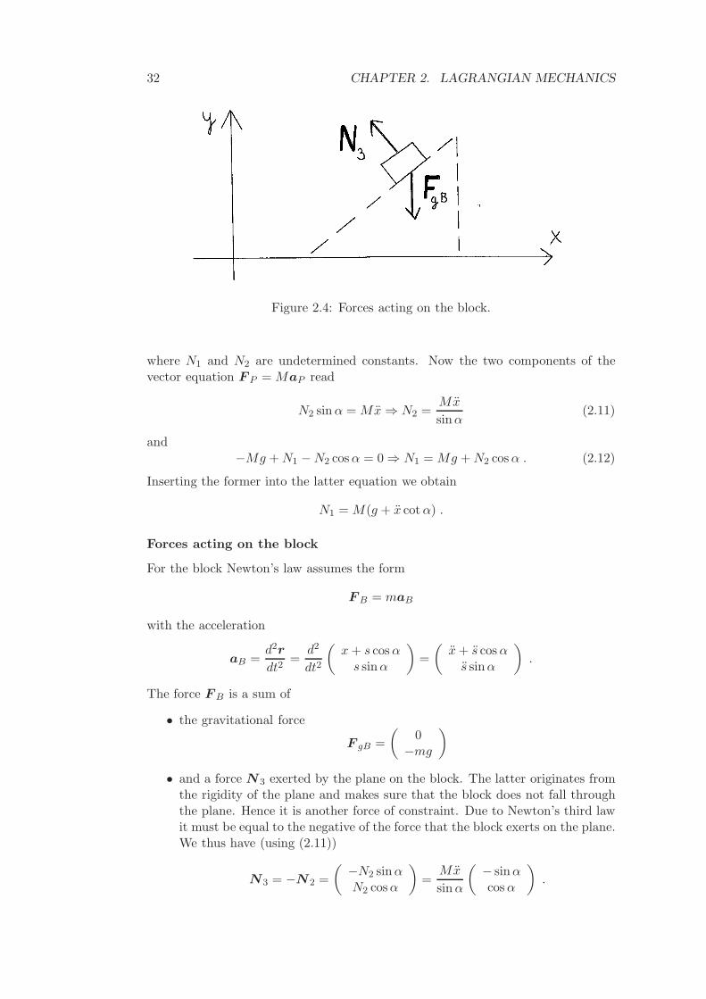
Figure 2.4: Forces acting on the block.
where N1 and N2 are undetermined constants. Now the two components of thevector equation F P = MaP read
N2 sin α = Mx ⇒ N2 =Mx
sinα(2.11)
and−Mg + N1 − N2 cos α = 0 ⇒ N1 = Mg + N2 cos α . (2.12)
Inserting the former into the latter equation we obtain
N1 = M(g + x cot α) .
Forces acting on the block
For the block Newton’s law assumes the form
F B = maB
with the acceleration
aB =d2r
dt2=
d2
dt2
(x + s cos α
s sinα
)
=
(x + s cos α
s sinα
)
.
The force F B is a sum of
• the gravitational force
F gB =
(0
−mg
)
• and a force N 3 exerted by the plane on the block. The latter originates fromthe rigidity of the plane and makes sure that the block does not fall throughthe plane. Hence it is another force of constraint. Due to Newton’s third lawit must be equal to the negative of the force that the block exerts on the plane.We thus have (using (2.11))
N3 = −N 2 =
(−N2 sin αN2 cos α
)
=Mx
sin α
(− sinαcos α
)
.
2.3. GENERALISED COORDINATES AND CONSTRAINTS 33
Summation yields the overall force
F B = F gB + N 3 =
(−Mx
−mg + Mx cot α
)
.
Now the two components of Newton’s law read
m(x + s cos α) = −Mx
⇒ x = − m
m + Ms cos α (2.13)
and
ms sinα = −mg + Mx cot α
= −mg − mM
m + Mscos2 α
sin α(2.14)
(where in the last step we used Eq. (2.13)). If we multiply Eq. (2.14) with sin αm+Mm
we obtain
(m + M)s sin2 α = −(m + M)g sin α − Ms cos2 α
⇒ (m sin2 α + M)s = −(m + M)g sin α
⇒ s = −(M + m)g sin α
M + m sin2 α= const . (2.15)
Substitution into (2.13) then yields
x =mg
M + m sin2 αsinα cos α = const. (2.16)
Discussion
We see that Lagrange’s equations and Newton’s law yield coinciding results, givenin Eqs. (2.9), (2.10) and in Eqs. (2.15), (2.16). The Lagrangian treatment isconsiderably simpler since we can build in the constraints by appropriately choosingcoordinates. In the Newtonian approach we instead have to take into accountadditional forces. These forces N 1, N 2, N 3 are forces of constraint. They keepthe block on the plane and the plane on the table. These forces don’t appear in theLagrangian treatment. However we can always determine them if we want (e.g., ifwe need the force exerted on the table to see if it breaks). We then have to solveLagrange’s equations and determine determine the forces of constraint from mri
and the known conservative forces F pot as in
miri = Fpoti + F constraint
i
⇒ F constrainti = F
poti − miri .
2.3.4 General properties of forces of constraint
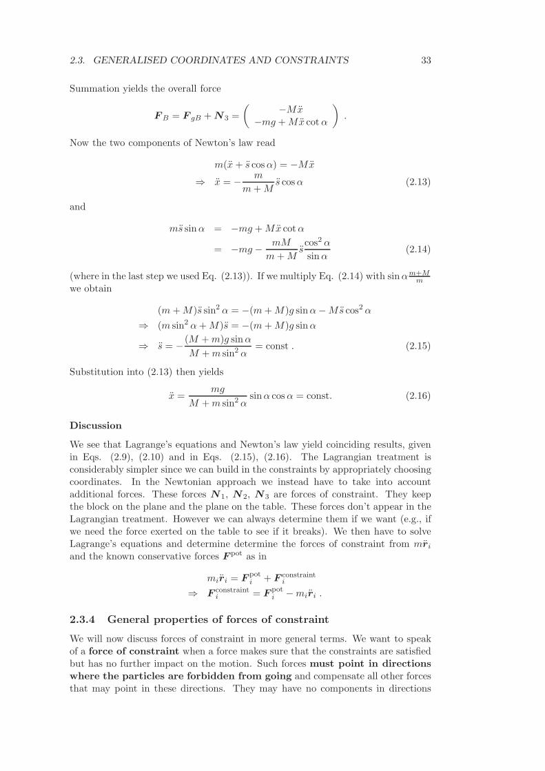
We will now discuss forces of constraint in more general terms. We want to speakof a force of constraint when a force makes sure that the constraints are satisfiedbut has no further impact on the motion. Such forces must point in directionswhere the particles are forbidden from going and compensate all other forcesthat may point in these directions. They may have no components in directions
34 CHAPTER 2. LAGRANGIAN MECHANICS
where the particles are allowed to go. An example is the normal force N 1 in theexample of the inclined plane, see Fig. 2.5. This force points in the direction normalto the table, and compensates the gravitational force and the force from the blockwhich push the inclined plane into a forbidden direction.
Figure 2.5: Example for a force of constraint.
Allowed and forbidden directions
To formulate the above condition mathematically we have to look in more detail atthe directions in which a system is, or is not, allowed to move.
• First of all we note that all particle positions (r1, . . . , rN ) form a 3N -dimensionalspace (or a 2N -dimensional space if the position vectors are in R
2).
• However not all positions are allowed. We parametrize the allowed positionsof particles by d generalised coordinates q1, . . . , qd and (possibly) time as
ri = ri(q1, . . . , qd, t) .
This defines the d-dimensional configuration space.
• Starting from an allowed (r1, . . . , rN ) we can go into all directions in the3N -dimensional space that can be reached by changing the q1, . . . , qd. Forinstance, if we change qα by an infinitesimal amount δqα, each particle positionri changes by δri = ∂ri
∂qαδqα. This means that all infinitesimal motions in the
3N -dimensional space that go in directions
(∂r1
∂qα, . . . ,
∂rN
∂qα
)
(2.17)
are allowed. The same applies to linear combinations of these directions.At every point (r1, . . . , rN ) there are d directions as in (2.17), one for eachα = 1, . . . , d.
• This leaves 3N − d linearly independent forbidden directions (one for eachconstraint). They are perpendicular to the allowed directions.
Now consider a set of forces (F c1,F
c2, . . . ,F
cN ), where F c
1 acts on the first particle,F c
2 acts on the second particle, etc. These forces are forces of constraint if the 3N -dimensional vector (F c
1,Fc2, . . . ,F
cN ) points into a forbidden direction (such that
other forces pointing into these directions are compensated) and is perpendicular to
2.3. GENERALISED COORDINATES AND CONSTRAINTS 35
the allowed directions (such that the motion in allowed directions is not affected).This means that the scalar product of (F c
1,Fc2, . . . ,F
cN ) and any of the allowed
directions must vanish. Forces of constraint can thus be defined as follows:
Definition (D’Alembert’s principle)
A set of forces (F c1,F
c2, . . . ,F
cN ) are forces of constraint if we have
(F c1,F
c2, . . . ,F
cN ) ·
(∂r1
∂qα, . . . ,
∂rN
∂qα
)
=
N∑
i=1
F ci ·
∂ri
∂qα= 0 (2.18)
for all α = 1 . . . d
Note: The term “allowed direction” used here is not standard. Traditionally,these allowed directions are rather referred to a “virtual displacements”. Fur-thermore note that the left-hand side of Eq. (2.18) has the dimension of work,since it involves a product of forces and changes of positions. The traditional wayof stating D’Alembert’s principle is thus to say that virtual displacements do nowork.
2.3.5 Derivation of Lagrange’s equations from Newton’s law in thegeneral case
We have now learnt enough about constraints to give a proof for Lagrange’s equa-tions and the principle of least action for generalised coordinates and systemswith constraints. We will see that d’Alembert’s principle is crucial for showingthat forces of constraint don’t spoil the picture.
We consider systems where all forces are either conservative forces or forces ofconstraint. For these systems Newton’s second law reads:
miri = F i = −∂U
∂ri+ F c
i (2.19)
where F i is the overall force acting on the i-th particle. It is written as a sumof the conservative force − ∂U
∂riand the force of constraint F c
i . We now want toshow that Lagrange’s equations hold as well. I.e., if we parametrise the particlepositions by generalised coordinates where the constraint are automatically builtin,
ri = ri(q1, . . . , qd, t), (2.20)
then we have∂L
∂qα− d
dt
∂L
∂qα= 0 (2.21)
for all α = 1 . . . d. This means that Hamilton’s principle holds, i.e., that particlestravel on trajectories for which the action S =
∫Ldt becomes extremal.
Preparation: Formulas for partial derivatives of ri
To prepare for a proof, we first derive formulas for the derivatives of the velocitiesri w.r.t. the generalised coordinates qα and their derivatives qα. In Eq. (2.4) we
36 CHAPTER 2. LAGRANGIAN MECHANICS
took the derivative ofri = ri(q1, . . . , qd, t) , (2.22)
using the chain rule, and got
ri =dri
dt=
d∑
β=1
∂ri
∂qβ(q1, . . . , qd, t)qβ +
∂ri
∂t(q1, . . . , qd, t) . (2.23)
We thus expressed the velocity as a function
ri = ri(q1, . . . , qd, q1, . . . , qd, t) .
We can now take derivatives of ri w.r.t. generalised coordinates and qβ’s. If welook at (2.23) we see that the derivative w.r.t. qβ is just the term multiplying qβ.We thus have
∂ri
∂qβ=
∂ri
∂qβ. (2.24)
Since the two dots on the left-hand side have disappeared on the right-hand side,this rule is also known as the “cancellation of dots”. For the derivatives w.r.t.generalised coordinates we will show that
∂ri
∂qα=
d
dt
∂ri
∂qα. (2.25)
This means that the total derivative w.r.t. t (which appears on the left-hand sideas a dot) and the partial derivative w.r.t. qα can be interchanged – which would betrivial if both derivatives were partial, but it is necessary to give a proof becauseone of the derivatives is a total one.
Proof: To evaluate the l.h.s., we use (2.23). The only qα-dependent terms in(2.23) are ∂ri
∂qβand ∂ri
∂t . Hence the chain rule yields
∂ri
∂qα=
d∑
β=1
∂2ri
∂qα∂qβqβ +
∂2ri
∂qα∂t.
To compute the term ddt
∂ri
∂qαon the r.h.s., we use ∂ri
∂qαis a function of the generalised
coordinates and time. Hence the chain rule brings about partial derivatives withrespect to these quantities, and the final result
d
dt
∂ri
∂qα=
d∑
β=1
∂2ri
∂qα∂qβqβ +
∂2ri
∂qα∂t
agrees with the left-hand side. Eq. (2.25) is thus proven.
Strategy
We are now ready to prove Lagrange’s equation. We start from Newton’s law,multiply both sides with ∂ri
∂qα, and sum over i. This yields
N∑
i=1
miri∂ri
∂qα=
N∑
i=1
(
−∂U
∂ri+ F c
i
)
︸ ︷︷ ︸
=F i
· ∂ri
∂qα. (2.26)
2.3. GENERALISED COORDINATES AND CONSTRAINTS 37
A motivation for this strategy is that we would like to get an expression that involvespartial derivatives w.r.t. qα – hence it is a good idea to multiply with ∂ri
∂qα. We now
have to simplify all three terms obtained to get Lagrange.
Acceleration term
For the first term involving the acceleration ri, we pull one of the two time deriv-atives in front such that is also acts on ∂ri
∂qα, and then subtract the term where the
time derivative acts on ∂ri
∂qα,
N∑
i=1
miri ·∂ri
∂qα=
N∑
i=1
mi
[d
dt
(
ri ·∂ri
∂qα
)
− ri ·d
dt
∂ri
∂qα
]
.
We then use Eq. (2.24) for the first term, and Eq. (2.25) for the second term,
N∑
i=1
miri ·∂ri
∂qα=
N∑
i=1
mi
d
dt
(
ri ·∂ri
∂qα
)
︸ ︷︷ ︸
= 12
∂∂qα
r2i
− ri ·∂ri
∂qα︸ ︷︷ ︸
= 12
∂∂qα
r2i
(2.27)
As indicated in Eq. (2.27), the terms ri · ∂ri
∂qαand ri · ∂ri
∂qαthus obtained can be
written as derivatives of r2i . This is reassuring since r2
i shows up in the kineticenergy T included in L. We may thus hope to obtain derivatives of T . To do so wenow pull all derivatives in front which leads to
N∑
i=1
miri ·∂ri
∂qα=
d
dt
∂
∂qα
N∑
i=1
1
2mir
2i −
∂
∂qα
N∑
i=1
1
2mir
2i .
We now recognise∑N
i=112mir
2i as the kinetic energy and write
N∑
i=1
miri ·∂ri
∂qα=
d
dt
∂T
∂qα− ∂T
∂qα.
We have thus expressed the first term in (2.26) through derivatives of the kineticenergy, and obtained the intermediate result
d
dt
∂T
∂qα− ∂T
∂qα=
N∑
i=1
F i ·∂ri
∂qα. (2.28)
In Eq. (2.28) we have not yet used our assumptions on the forces (i.e. that they aresums of conservative forces and forces of constraint). Eq. (2.28) can thus be seenas a generalisation of Lagrange’s equation for arbitrary forces.
Potential term
The derivative of the potential in Eq. (2.26), multiplied with ∂ri
∂qαand summed over,
simply gives
−N∑
i=1
∂U
∂ri· ∂ri
∂qα= − ∂U
∂qα
– again a term that we would like to see in Lagrange’s equation!
38 CHAPTER 2. LAGRANGIAN MECHANICS
Constraint term
The final term in (2.26) readsN∑
i=1
F ci ·
∂ri
∂qα
This is exactly the scalar product of forces of constraint and allowed directions(2.18) that vanishes due to d’Alembert’s principle. We thus have
N∑
i=1
F ci ·
∂ri
∂qα= 0 ,
and we see that due to d’Alembert’s principle the forces of constraint drop from ourequations of motion.
Result
Summation of all three terms yields
d
dt
∂T
∂qα− ∂T
∂qα= − ∂U
∂qα
⇒ ∂(T − U)
∂qα− d
dt
∂T
∂qα= 0
which is suspiciously close to Lagrange’s equations for L = T − U . The onlything that one might miss is a derivative d
dt∂U∂qα
. But by definition, the potential
is independent of qα and thus ddt
∂U∂qα
= 0. If we now simply add ddt
∂U∂qα
and replaceT − U by L, we obtain our desired result:
Lagrange’s equation
∂L
∂qα− d
dt
∂L
∂qα= 0 for all α = 1, . . . , d
2.4. CONSERVED QUANTITIES 39
2.4 Conserved quantities
In mechanics it is often helpful to look for conserved quantities and for examplecheck whether the energy, the momentum or the angular momentum of a particleremains fixed.
Def.: A quantity A is a conserved if the total time derivative dAdt vanishes.
We will show that Lagrangian mechanics provides an ideal framework to studythese conserved quantities. In particular we will see that conserved quantities alwaysarise when the Lagrangian is independent of one of the arguments q1, . . . , qd, t.
2.4.1 Energy conservation
First of all we will show that if the Lagrangian does not depend on time, the so-calledgeneralised energy is conserved. (Usually this is just the energy itself.)
Conservation of the generalised energy
If the Lagrangian of a system is independent of the time t, i.e.,
L = L(q1, . . . , qd︸ ︷︷ ︸
=q
, q1, . . . , qd︸ ︷︷ ︸
=q
)
then the generalised energy
h ≡d∑
α=1
∂L
∂qαqα − L =
∂L
∂q· q − L
is a conserved quantity.
Note that here we used the vector notation q = (q1, . . . , qd) for the generalisedcoordinates.
Proof
• Remembering variational calculus we can use the alternative version ofthe Euler-Lagrange equation. We had seen that if a function f = f(y,y′)is independent of x, then the functional K =
∫ x2
x1f(y(x),y′(x))dx becomes
stationary if
∂f
∂y′ · y′ − f = const.
(Here the sign of the constant is flipped compared to section 1.) Thus theEuler-Lagrange equation was directly formulated in terms of a conservationlaw. To apply this result to Lagrangian mechanics, we replace x → t, y → q,f → L and K → S. Then we immediately obtain the statement above.
• Since it was so simple, we can just redo the proof and take the total derivative
40 CHAPTER 2. LAGRANGIAN MECHANICS
of h:
dh
dt=
d
dt
(∂L
∂q· q)
− dL
dt
=
(d
dt
∂L
∂q
)
· q +∂L
∂q· q − ∂L
∂qq − ∂L
∂q· q
If we use Lagrange’s equations to replace ddt
∂L∂q
by ∂L∂q
we see that all termsabove cancel and thus
dh
dt= 0 .
Example
Let us consider the motion of a particle in one dimension. The correspondingLagrangian
L =1
2mx2 − U(x)
does not depend explicitly on time. Hence the generalised energy must be conserved;it reads
h =∂L
∂xx − L
= mxx −(
1
2mx2 − U(x)
)
=1
2mx2 + U(x) (2.29)
which is just the sum of kinetic and potential energy, i.e., the energy E = T + Uitself.
I now want to show that this result h = E actually generalises to most practicalcases (albeit there are exceptions). To check this we first need an explicit formulafor the Lagrangian, and in particular for the kinetic energy of a mechanical system.We can then compute h and see whether it agrees with E.
General formula for the kinetic energy
If we use Cartesian coordinates for the particle positions ri, the kinetic energy of amechanical system always has the form
T =
N∑
i=1
1
2mir
2i . (2.30)
We now want to see how this formula looks if we use generalised coordinatesq1, . . . , qd. The particle positions can then be parametrised by these generalisedcoordinates and (possibly) time as
ri = ri(q1, . . . , qd, t) .
According to the chain rule the velocity turns into
ri =d∑
α=1
∂ri
∂qαqα +
∂ri
∂t. (2.31)
2.4. CONSERVED QUANTITIES 41
If we insert this into the above formula for T we get
T =
N∑
i=1
1
2mi
d∑
α=1
∂ri
∂qαqα ·
d∑
β=1
∂ri
∂qβqβ + 2
d∑
α=1
∂ri
∂qαqα · ∂ri
∂t+
(∂ri
∂t
)2
. (2.32)
This follows directly by inserting (2.31) into (2.30); the only nontrivial point isthat when squaring
∑dα=1
∂ri
∂qαqα I wrote the two factors with different summation
variables α and β to make clear that there are two different sums, not just one.It would be nice if we could write Eq. (2.32) in a less clunky way. To do so weabbreviate the terms that are not derivatives of q by
Mαβ(q1, . . . , qd, t) ≡N∑
i=1
mi∂ri
∂qα· ∂ri
∂qβ
vα(q1, . . . , qd, t) ≡N∑
i=1
mi∂ri
∂qα· ∂ri
∂t
c(q1, . . . , qd, t) ≡N∑
i=1
mi
(∂ri
∂t
)2
. (2.33)
The kinetic energy then turns into
T =1
2
N∑
α=1
N∑
β=1
Mαβ qαqβ +
d∑
α=1
vαqα +c
2. (2.34)
To make this result even more compact we adopt a vector and matrix notation. Wethus collect all Mαβ’s into a matrix
M ≡
M11 . . . M1d...
...Md1 . . . Mdd
and all vα’s into a vector
v =
v1...vd
.
Here M is a symmetric matrix (Mαβ = Mβα) because the matrix elements Mαβ
defined above remain the same if α and β are interchanged. With this M and v thekinetic energy assumes the form:
General formula for the kinetic energy
T =1
2q · M q + v · q +
c
2(2.35)
The term quadratic in q, 12 q · M q, looks very much like the usual formula for
the kinetic energy of a single particle in Cartesian coordinates. The only differencesare that q is a vector containing derivatives of generalised coordinates, and that the
42 CHAPTER 2. LAGRANGIAN MECHANICS
mass is replaced by a matrix that may depend on q. This matrix is alsocalled the mass matrix.
The linear and constant terms are new. However they show up only if ourtransformation between Cartesian and generalised coordinates involves time, i.e.,if ri = (q1, . . . , qd, t) with ∂ri
∂t 6= 0. In the usual situation that there is no time
dependence, we have ∂ri
∂t = 0 and the vα and c defined in (2.33) simply vanish.Then we only have the quadratic term.
Formulas for gradients of linear and quadratic functions
To get h we must evaluate derivatives of L = T − U w.r.t. q and q, i.e., we mustlearn how to deal with derivatives of scalar products like v · q and quadratic termslike q · M q with respect to the vectors involved. We recall that the derivative(gradient) w.r.t. a vector u is defined as the vector containing partial derivativesw.r.t. the components of u, i.e.,
∂f
∂u=
∂f∂u1...
∂f∂ud
.
We will show that derivatives of such terms are given by
∂(v · u)
∂u= v (2.36)
∂(u · Mu)
∂u= 2Mu if M is symmetric (2.37)
which are just the formulas we would get if v, u and M were scalars.
Proof of (2.36): We use that
v · u =
d∑
α=1
vαuα .
The partial derivatives are thus given by
∂(v · u)
∂uα= vα
and collecting them into a vector yields v as in (2.36).
Proof of (2.37): We use that
u · Mu =
d∑
α=1
d∑
β=1
Mαβuαuβ .
The partial derivatives are thus given by
∂(u · Mu)
∂uγ=
d∑
α=1
d∑
β=1
Mαβ
(∂uα
∂uγuβ + uα
∂uβ
∂uγ
)
. (2.38)
2.4. CONSERVED QUANTITIES 43
Here the derivative ∂uα
∂uγreads
∂uα
∂uγ= δαγ ≡
1 if α = γ
0 otherwise
Therefore the first sum in (2.38) only receives contributions when α = γ. We thus
drop ∂uα
∂uγand the summation over α and replace the remaining α by γ. The
∂uβ
∂uγin
the second term is handled in an analogous way. We then obtain
∂(u · Mu)
∂uγ=
d∑
β=1
Mγβuβ +d∑
α=1
Mαγuα .
If we now rename the summation variable α in the second sum into β and use thatM is symmetric (Mβγ = Mγβ) we get
∂(u · Mu)
∂uγ=
d∑
β=1
Mγβuβ +
d∑
β=1
Mβγ︸︷︷︸
=Mγβ
uβ = 2
d∑
β=1
Mγβuβ
Collecting all partial derivatives ∂(u·Mu)∂uγ
into a vector we thus get 2Mu as claimed.
Generalised energy
We are now prepared to evaluate the generalised energy. Due to (2.35) the La-grangian is given by
L =1
2q · M q + v · q +
c
2− U .
The generalised energy can now be computed from (2.29),
h =∂L
∂q· q − L
= (M q + v) · q − 1
2q · M q − v · q − c
2+ U
=1
2q · M q − c
2+ U
For comparison, the energy is
E = T + U =1
2q · M q + v · q +
c
2+ U .
So the good news is:
If the kinetic energy is quadratic in q, i.e. v = 0 and c = 0, then theenergy coincides with the generalised energy
This is the generic situation that we have if the transformation between Carte-sian and generalised coordinates is time independent and thus ∂ri
∂t = 0. (Also recallthat U is independent of q.)
In a practical example we would first check whether L depends on t or not. Ifit is independent, h is conserved. If T is quadratic in q we simply have h = E,otherwise we need to calculate h explicitly.
44 CHAPTER 2. LAGRANGIAN MECHANICS
Example where these conditions are satisfied:
For the inclined plane we had
L = T − U =
(1
2(M + m)x2 +
1
2ms2 + mxs cos α
)
− mgs sin α .
(Here I renamed the mass of the plane into M to avoid confusion with the matrixM). L is independent of t, hence h is conserved. All terms in T involve products oftwo factors x or s. Therefore the generalised energy coincides with the energy andwe have
h = E = T + U =
(1
2(M + m)x2 +
1
2ms2 + mxs cos α
)
+ mgs sin α .
Examples where these conditions are violated:
• Consider a pendulum fixed to a point (0, y(t)) that is moving depend-ing on time with y(t) = y0 sinωt. Using θ (see Fig. 2.6) as a generalisedcoordinate, we can write
r(θ, t) =
(0
y(t)
)
+ l
(sin θ
− cos θ
)
,
i.e. the potential is
U = mg(y(t) − l cos θ) .
If we take the derivative
r =
(0
y(t)
)
+ lθ
(cos θsin θ
)
we get the kinetic energy
T =1
2mr2 =
1
2m(l2θ2 + 2l sin θθy(t) + y(t)2)
and the Lagrangian
L(θ, θ, t) = T − U =1
2m(l2θ2 + 2l sin θθy(t) + y(t)2) − mg(y(t) − l cos θ) .
L depends explicitly on t, so h is not conserved. Moreover the kinetic en-ergy contains terms linear in θ and independent of θ. (Note that y is not ageneralised coordinate so θy and y2 do not count as quadratic terms!) Henceour condition for h = E = T + U is violated and we have to compute thegeneralised energy using
h =∂L
∂θθ − L =
1
2m(l2θ2 − y(t)2) + mg(y(t) − l cos(θ)) 6= T + U .
• Another example (that will be on problem sheet 4) involves a particle in amagnetic field. In this example a term linear in q arises such that h 6= E.However, L is independent of t, so h is still conserved.
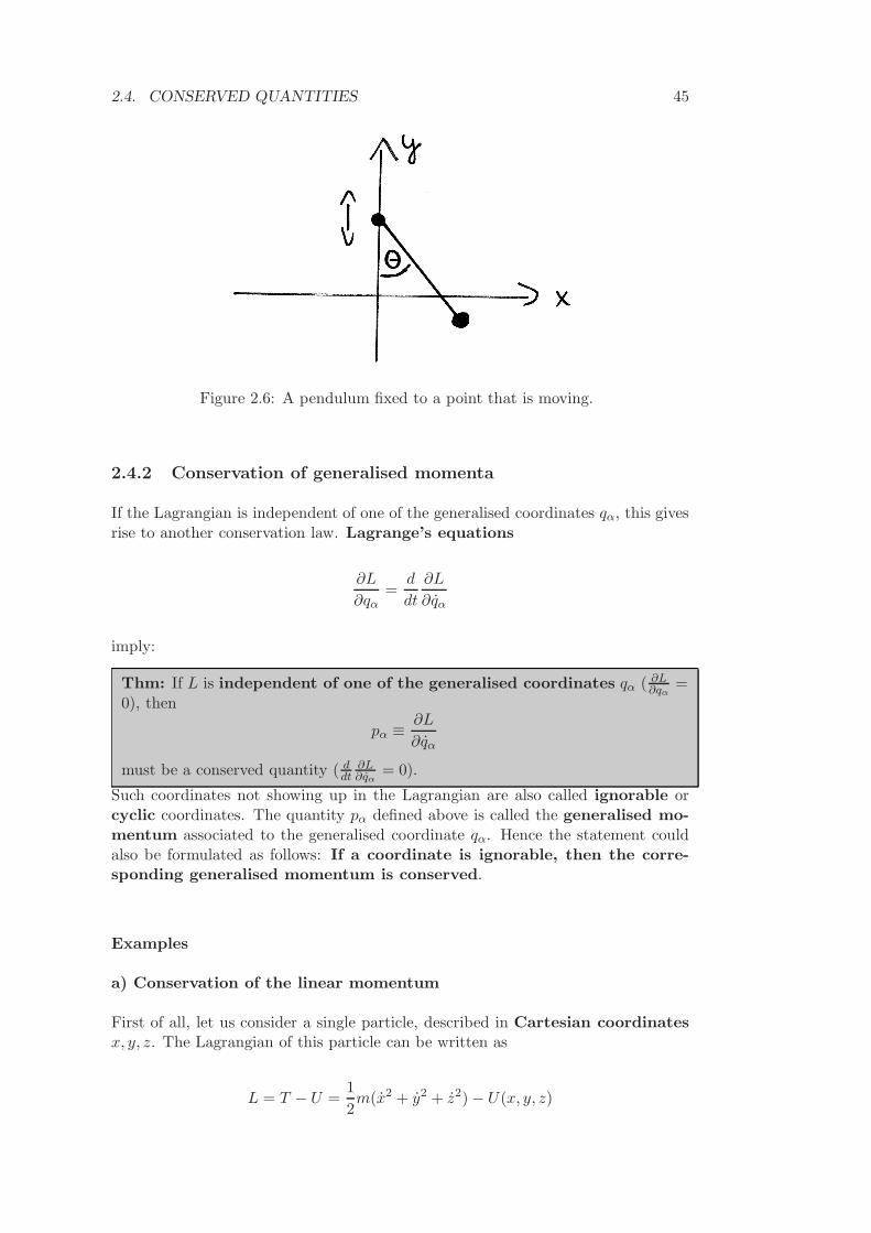
2.4. CONSERVED QUANTITIES 45
Figure 2.6: A pendulum fixed to a point that is moving.
2.4.2 Conservation of generalised momenta
If the Lagrangian is independent of one of the generalised coordinates qα, this givesrise to another conservation law. Lagrange’s equations
∂L
∂qα=
d
dt
∂L
∂qα
imply:
Thm: If L is independent of one of the generalised coordinates qα ( ∂L∂qα
=0), then
pα ≡ ∂L
∂qα
must be a conserved quantity ( ddt
∂L∂qα
= 0).
Such coordinates not showing up in the Lagrangian are also called ignorable orcyclic coordinates. The quantity pα defined above is called the generalised mo-mentum associated to the generalised coordinate qα. Hence the statement couldalso be formulated as follows: If a coordinate is ignorable, then the corre-sponding generalised momentum is conserved.
Examples
a) Conservation of the linear momentum
First of all, let us consider a single particle, described in Cartesian coordinatesx, y, z. The Lagrangian of this particle can be written as
L = T − U =1
2m(x2 + y2 + z2) − U(x, y, z)
46 CHAPTER 2. LAGRANGIAN MECHANICS
where U(x, y, z) is the potential. Now the generalised momenta px, py and pz
associated to x, y and z are obtained as
px =∂L
∂x= mx
py =∂L
∂y= my
pz =∂L
∂z= mz .
We thus see that these generalised momenta just coincide with the usual (linear)momenta in x-, y- and z-direction, mass times component of the velocity.
We now obtain the following conservation law: If the potential and thusLagrangian are independent of x,
∂L
∂x= −∂U
∂x= 0 ,
then the momentum in x-direction px = mx is conserved. Analogous results holdfor py and pz.
Within Newtonian mechanics, we would have argued that due to ∂U∂x = 0 there
is no force in x-direction and hence the corresponding component of the momentumremains constant.
b) Angular momentum conservation
Let us now see what happens if we are in the x− y−plane and instead of Cartesiancoordinates pick polar coordinates,
r = ρ
cos φsin φ
0
.
We then have
r = ρ
cos φsin φ
0
+ ρφ
− sin φcos φ
0
and thusr2 = ρ2 + ρ2φ2 .
The Lagrangian reads
L = T − U =1
2m(ρ2 + ρ2φ2) − U(ρ, φ)
where the potential was written as a general function of ρ and φ. So what are thegeneralised momenta associated to ρ and φ? For ρ we get
pρ =∂L
∂ρ= mρ
which is of the same type as the linear momenta, but now with the velocity ρ. Hencepρ can be interpreted as the radial component of the linear momentum. Thegeneralised momentum associated to φ reads
pφ =∂L
∂φ= mρ2φ .
2.4. CONSERVED QUANTITIES 47
pφ has the interpretation of an angular momentum. To check this, we use thedefinition of the angular momentum l = r×p = r×mr from Mechanics 1. Insertingour formula for r and r we obtain
l = ρ
cos φsin φ
0
×
mρ
cos φsinφ
0
+ mρφ
− sin φcos φ
0
=
00
mρ2φ
.
The only interesting component here is the z-component. (Any cross product of twovectors in the x − y−plane must point in z-direction.) As anticipated it coincideswith pφ.
Now which conservation law do we get? Since the kinetic energy already dependson ρ, the radial coordinate cannot be ignorable. But φ can be ignorable, if thepotential U depends only on ρ and not on φ,
∂L
∂φ= −∂U
∂φ= 0 .
In this case the angular momentum is conserved. Such potentials independentof φ are also referred to as central fields. Central fields are rather common. If wehave, e.g., a gravitational field due to a mass at the origin, the potential will onlydepend on the distance ρ from the origin.
c) Inclined plane
For the inclined plane we have
L = T − U =1
2(M + m)x2 +
1
2ms2 + mxs cos α − mgs sin α .
and the generalised momenta are
px =∂L
∂x= (M + m)x + ms cos α
ps =∂L
∂s= ms + mx cos α .
L is independent of x, hence px is conserved. But it depends on s, thus ps is notconserved.
2.4.3 Spherical pendulum
The spherical pendulum is a good example to illustrate the use of conservation lawsin Lagrangian mechanics. It is simply a pendulum that is allowed to move in allthree dimensions of space rather than in only two dimensions. To build a sphericalpendulum, one simply takes a particle of mass m and pivots at the origin by a rigidrod of length l. Since the particle is allowed to move in three-dimensional space butits distance from the origin is fixed to be l, the possible particle positions forma sphere of radius l around the origin. For simplicity, we will choose units inwhich m, g and l all become 1.
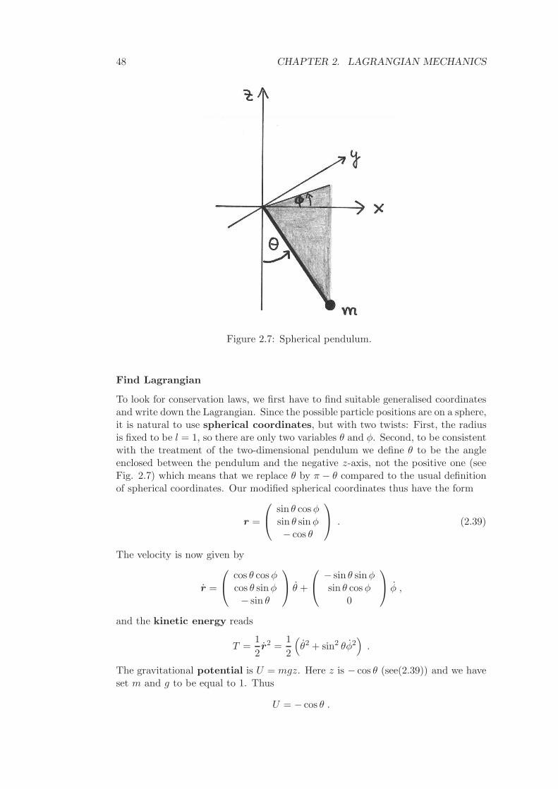
48 CHAPTER 2. LAGRANGIAN MECHANICS
Figure 2.7: Spherical pendulum.
Find Lagrangian
To look for conservation laws, we first have to find suitable generalised coordinatesand write down the Lagrangian. Since the possible particle positions are on a sphere,it is natural to use spherical coordinates, but with two twists: First, the radiusis fixed to be l = 1, so there are only two variables θ and φ. Second, to be consistentwith the treatment of the two-dimensional pendulum we define θ to be the angleenclosed between the pendulum and the negative z-axis, not the positive one (seeFig. 2.7) which means that we replace θ by π − θ compared to the usual definitionof spherical coordinates. Our modified spherical coordinates thus have the form
r =
sin θ cos φsin θ sin φ− cos θ
. (2.39)
The velocity is now given by
r =
cos θ cos φcos θ sin φ− sin θ
θ +
− sin θ sinφsin θ cos φ
0
φ ,
and the kinetic energy reads
T =1
2r2 =
1
2
(
θ2 + sin2 θφ2)
.
The gravitational potential is U = mgz. Here z is − cos θ (see(2.39)) and we haveset m and g to be equal to 1. Thus
U = − cos θ .
2.4. CONSERVED QUANTITIES 49
The Lagrangian therefore has the form
L =1
2θ2 +
1
2sin2 θφ2 + cos θ .
Conserved quantities
Now we want to look for conserved quantities, and thus for ignorable coordinates.The Lagrangian L does not depend on φ and t. This should give rise to two con-servation laws:
• Since L is independent of t, the generalised energy h is conserved. Sincethe kinetic energy is quadratic in the derivatives θ and φ the generalisedenergy also coincides with the energy E = T + U . Thus we also have energyconservation:
E = T + U =1
2θ2 +
1
2sin2 θφ2 − cos θ = const . (2.40)
• Since φ is ignorable, the corresponding generalised momentum pφ must be aconserved quantity. We thus have
pφ =∂L
∂φ= sin2 θφ = const. (2.41)
pφ can be identified with the z-component of the angular momentum(corresponding to rotations about the z-axis, which is the symmetry axis of thespherical pendulum). We had already seen that this is the right interpretationof the generalised momentum associated to φ in polar coordinates. Similarly,if we use spherical coordinates the z-component of the angular momentumr × mr (where m = 1) is given by
xy − yx
= sin θ cos φ(cos θ sin φθ + sin θ cos φφ) − sin θ sinφ(cos θ cos φθ − sin θ sinφφ)
= sin2 θφ
which indeed coincides with pφ.
Conservation laws are so valuable for the description of mechanical systemsbecause they allow us to reduce the number of independent variables. In thepresent case, we can use (2.41) to get rid of φ in (2.40). If we solve (2.41) for φ weget
φ =pφ
sin2 θ. (2.42)
Inserting this into (2.40) yields
E =1
2θ2 +
p2φ
2 sin2 θ− cos θ = const (2.43)
Now we have a differential equation for θ only. There is no φ because T and U areindependent of φ (which was the reason for angular momentum conservation inthe first place), and then φ could be eliminated using (2.41). Instead we have twoconstants, E and pφ.
50 CHAPTER 2. LAGRANGIAN MECHANICS
Interpretation
Since φ is gone, Eq. (2.43) could be interpreted as describing a fictitious particlein one dimension, with the only coordinate θ. If we assume that this particlefeels an effective potential of the form
Veff(θ) =p2
φ
2 sin2 θ− cos θ (2.44)
then Eq. (2.43) could be interpreted as an energy conservation law for ourparticle:
E =1
2θ2 + Veff(θ) = const (2.45)
Here the effective potential contains both the original potential U = − cos θ and an
extra termp2
φ
2 sin2 θthat originates from the φ2-term in the kinetic energy; this term
became part of the effective potential due to the elimination of φ.We can also take the total time derivative, leading to
0 =dE
dt= θθ + V ′
eff(θ)θ .
Division by θ then gives
θ = −V ′eff(θ) . (2.46)
This means that the acceleration of our fictitious particle is given by the negativederivative of the effective potential, as one would expect. (Recall that we have setthe mass equal to one.)
Method I: Integration
There are two ways to proceed further. The first one (which we won’t carry to theend here) is to view (2.45) as a differential equation for θ, and try to integrate it.We thus take (2.45) and solve for θ,
θ2 = 2(E − Veff(θ))
⇒ θ =√
2(E − Veff(θ))
We then use separation of variables. We write θ = dθdt as
dt =dθ
θ
and afterwards integrate on both sides. The integral over t goes from 0 to t, whereasthe integral over θ goes from θ(0) to θ(t). If we insert the explicit formula for θ thisyields
t =
∫ t
0dt =
∫ θ(t)
θ(0)
dθ
θ=
∫ θ(t)
θ(0)
dθ√
2(E − Veff(θ))
The solution of our problem is thus written as an integral. The evaluation of thisintegral is rather tricky, and outside the scope of this course. One would finally belead to so-called elliptic functions, a kind of special functions. One would then haveto solve for θ(t), and afterwards determine φ(t).
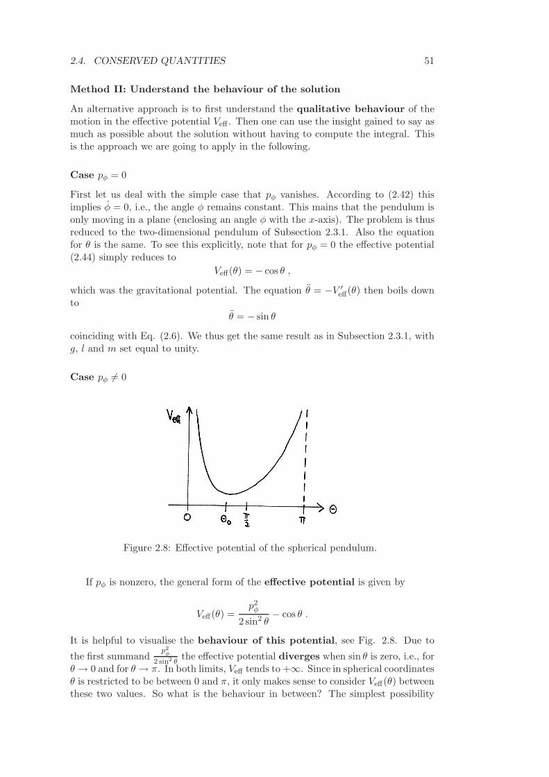
2.4. CONSERVED QUANTITIES 51
Method II: Understand the behaviour of the solution
An alternative approach is to first understand the qualitative behaviour of themotion in the effective potential Veff . Then one can use the insight gained to say asmuch as possible about the solution without having to compute the integral. Thisis the approach we are going to apply in the following.
Case pφ = 0
First let us deal with the simple case that pφ vanishes. According to (2.42) thisimplies φ = 0, i.e., the angle φ remains constant. This mains that the pendulum isonly moving in a plane (enclosing an angle φ with the x-axis). The problem is thusreduced to the two-dimensional pendulum of Subsection 2.3.1. Also the equationfor θ is the same. To see this explicitly, note that for pφ = 0 the effective potential(2.44) simply reduces to
Veff(θ) = − cos θ ,
which was the gravitational potential. The equation θ = −V ′eff(θ) then boils down
to
θ = − sin θ
coinciding with Eq. (2.6). We thus get the same result as in Subsection 2.3.1, withg, l and m set equal to unity.
Case pφ 6= 0
Figure 2.8: Effective potential of the spherical pendulum.
If pφ is nonzero, the general form of the effective potential is given by
Veff(θ) =p2
φ
2 sin2 θ− cos θ .
It is helpful to visualise the behaviour of this potential, see Fig. 2.8. Due to
the first summandp2
φ
2 sin2 θthe effective potential diverges when sin θ is zero, i.e., for
θ → 0 and for θ → π. In both limits, Veff tends to +∞. Since in spherical coordinatesθ is restricted to be between 0 and π, it only makes sense to consider Veff(θ) betweenthese two values. So what is the behaviour in between? The simplest possibility
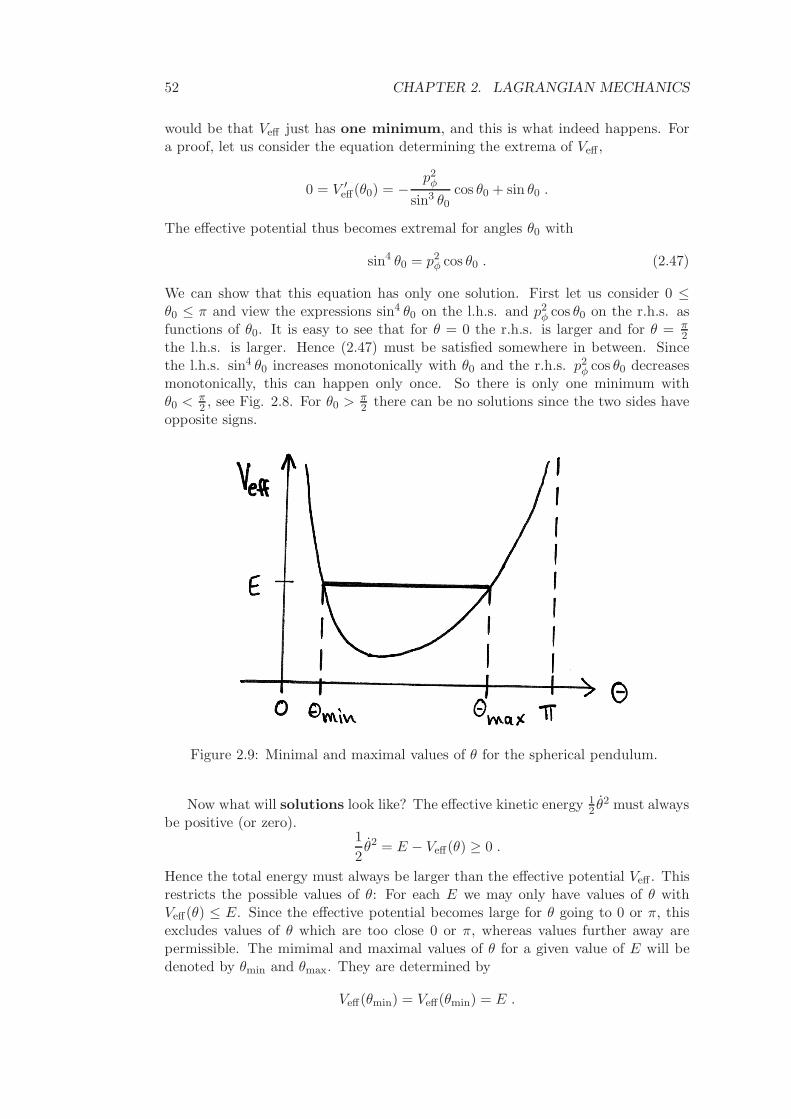
52 CHAPTER 2. LAGRANGIAN MECHANICS
would be that Veff just has one minimum, and this is what indeed happens. Fora proof, let us consider the equation determining the extrema of Veff ,
0 = V ′eff(θ0) = −
p2φ
sin3 θ0cos θ0 + sin θ0 .
The effective potential thus becomes extremal for angles θ0 with
sin4 θ0 = p2φ cos θ0 . (2.47)
We can show that this equation has only one solution. First let us consider 0 ≤θ0 ≤ π and view the expressions sin4 θ0 on the l.h.s. and p2
φ cos θ0 on the r.h.s. asfunctions of θ0. It is easy to see that for θ = 0 the r.h.s. is larger and for θ = π
2the l.h.s. is larger. Hence (2.47) must be satisfied somewhere in between. Sincethe l.h.s. sin4 θ0 increases monotonically with θ0 and the r.h.s. p2
φ cos θ0 decreasesmonotonically, this can happen only once. So there is only one minimum withθ0 < π
2 , see Fig. 2.8. For θ0 > π2 there can be no solutions since the two sides have
opposite signs.
Figure 2.9: Minimal and maximal values of θ for the spherical pendulum.
Now what will solutions look like? The effective kinetic energy 12 θ2 must always
be positive (or zero).1
2θ2 = E − Veff(θ) ≥ 0 .
Hence the total energy must always be larger than the effective potential Veff . Thisrestricts the possible values of θ: For each E we may only have values of θ withVeff(θ) ≤ E. Since the effective potential becomes large for θ going to 0 or π, thisexcludes values of θ which are too close 0 or π, whereas values further away arepermissible. The mimimal and maximal values of θ for a given value of E will bedenoted by θmin and θmax. They are determined by
Veff(θmin) = Veff(θmin) = E .
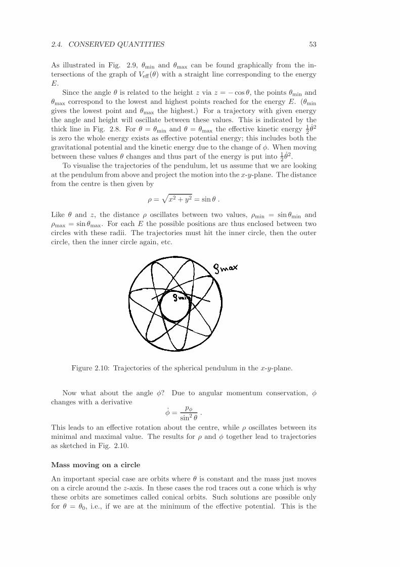
2.4. CONSERVED QUANTITIES 53
As illustrated in Fig. 2.9, θmin and θmax can be found graphically from the in-tersections of the graph of Veff(θ) with a straight line corresponding to the energyE.
Since the angle θ is related to the height z via z = − cos θ, the points θmin andθmax correspond to the lowest and highest points reached for the energy E. (θmin
gives the lowest point and θmax the highest.) For a trajectory with given energythe angle and height will oscillate between these values. This is indicated by thethick line in Fig. 2.8. For θ = θmin and θ = θmax the effective kinetic energy 1
2 θ2
is zero the whole energy exists as effective potential energy; this includes both thegravitational potential and the kinetic energy due to the change of φ. When movingbetween these values θ changes and thus part of the energy is put into 1
2 θ2.To visualise the trajectories of the pendulum, let us assume that we are looking
at the pendulum from above and project the motion into the x-y-plane. The distancefrom the centre is then given by
ρ =√
x2 + y2 = sin θ .
Like θ and z, the distance ρ oscillates between two values, ρmin = sin θmin andρmax = sin θmax. For each E the possible positions are thus enclosed between twocircles with these radii. The trajectories must hit the inner circle, then the outercircle, then the inner circle again, etc.
Figure 2.10: Trajectories of the spherical pendulum in the x-y-plane.
Now what about the angle φ? Due to angular momentum conservation, φchanges with a derivative
φ =pφ
sin2 θ.
This leads to an effective rotation about the centre, while ρ oscillates between itsminimal and maximal value. The results for ρ and φ together lead to trajectoriesas sketched in Fig. 2.10.
Mass moving on a circle
An important special case are orbits where θ is constant and the mass just moveson a circle around the z-axis. In these cases the rod traces out a cone which is whythese orbits are sometimes called conical orbits. Such solutions are possible onlyfor θ = θ0, i.e., if we are at the minimum of the effective potential. This is the
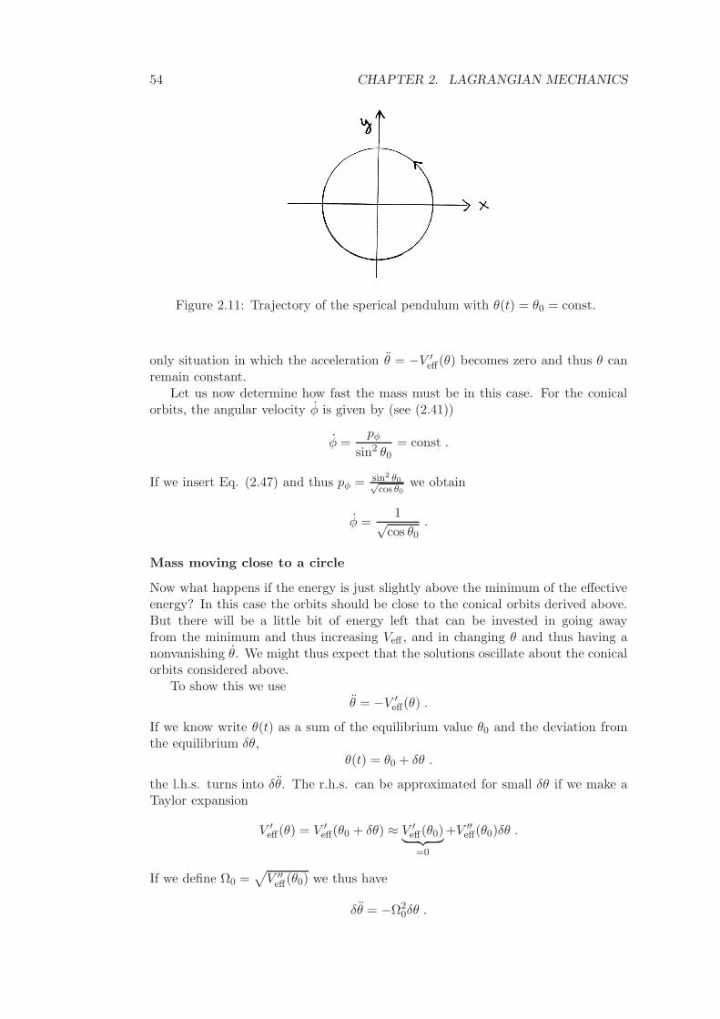
54 CHAPTER 2. LAGRANGIAN MECHANICS
Figure 2.11: Trajectory of the sperical pendulum with θ(t) = θ0 = const.
only situation in which the acceleration θ = −V ′eff(θ) becomes zero and thus θ can
remain constant.Let us now determine how fast the mass must be in this case. For the conical
orbits, the angular velocity φ is given by (see (2.41))
φ =pφ
sin2 θ0= const .
If we insert Eq. (2.47) and thus pφ = sin2 θ0√cos θ0
we obtain
φ =1√
cos θ0.
Mass moving close to a circle
Now what happens if the energy is just slightly above the minimum of the effectiveenergy? In this case the orbits should be close to the conical orbits derived above.But there will be a little bit of energy left that can be invested in going awayfrom the minimum and thus increasing Veff , and in changing θ and thus having anonvanishing θ. We might thus expect that the solutions oscillate about the conicalorbits considered above.
To show this we use
θ = −V ′eff(θ) .
If we know write θ(t) as a sum of the equilibrium value θ0 and the deviation fromthe equilibrium δθ,
θ(t) = θ0 + δθ .
the l.h.s. turns into δθ. The r.h.s. can be approximated for small δθ if we make aTaylor expansion
V ′eff(θ) = V ′
eff(θ0 + δθ) ≈ V ′eff(θ0)︸ ︷︷ ︸
=0
+V ′′eff(θ0)δθ .
If we define Ω0 =√
V ′′eff(θ0) we thus have
δθ = −Ω20δθ .
2.4. CONSERVED QUANTITIES 55
This is the same differential equation as for a harmonic oscillator. The solutioninvolves sines or cosines with a frequency Ω0. In other words:
For orbits close to the conical orbits the angle θ of the spherical pendulum oscillateswith a frequency Ω0 =
√V ′′
eff(θ0).
(Recall that we have set m = 1, otherwise there would be a mass here as well.)
A simple calculation of the second derivative3 yields
Ω0 =
√
3 cos θ0 +1
cos θ0.
Due to cos θ0 > 0 this is larger than φ = 1√cos θ0
. Hence the radial oscillations
compared to the conical orbits are faster than the oscillation of the angle φ due torotation.
In a more general context the motion close to extrema of a potential (equilibria)will be discussed in Chapter 3.
2.4.4 Noether’s theorem
So far we have seen that conserved quantities arise when one of the the generalisedcoordinates qα or the time t don’t show up in the Lagrangian. This is an example fora more general principle: In fact all symmetries of a system and its Lagrangian giverise to conservation laws. This principle will be very helpful to get counterparts forthe conservation of linear and angular momenta (see Subsection 2.4.2) in a systemwith many particles. We will first study a further example and then generalise.
Translation symmetry
Consider a system with N particles at r1, . . . , rN . This system is called symmet-ric (or invariant) w.r.t. translations in direction d if the the Lagrangianremains the same when all particles positions are shifted by an arbitrary amountin direction d. This means that we have
L(r1, . . . , rN , r1, . . . , rN , t) = L(r1 + sd, . . . , rN + sd, r1, . . . , rN , t)
for all real numbers s.
Example: Consider the two-particle system with the Lagrangian
L(r1, r2, r1, r2) =1
2m1r
2 +1
2m2r
22 +
Gm1m2
|r1 − r2|, (2.48)
accounting for the kinetic energy of these particles and the potential due to theirgravitational attraction. Both the derivatives r1, r2 and the difference |r1 − r2|remain the same if all positions are increased by sd. Hence the Lagrangian is notchanged if both particles are moved in direction d.
Now our statement is:
3One has to show that V ′′eff(θ) =
3p2
φ
sin4 θcos2 θ +
p2
φ
sin2 θ+ cos θ. The result then follows if we insert
θ = θ0 and p2φ = sin4 θ0
cos θ0from Eq. (2.47).
56 CHAPTER 2. LAGRANGIAN MECHANICS
Thm.: For s system that is invariant w.r.t. translations in direction d the com-ponent of the total linear momentum of all particles
∑Ni=1 pi in direction d is
a conserved quantity, i.e.,N∑
i=1
pi · d = const.
Proof: For such a system L(r1 + sd, . . . , rN + sd, r1, . . . , rN , t) does not dependon s, which means that the derivative of L w.r.t. s vanishes. This is true for all s,but it will be sufficient to consider the derivative at s = 0. We then get
0 =∂
∂sL(r1 + sd, . . . , rN + sd, r1, . . . , rN , t)
∣∣s=0
=
N∑
i=1
∂L
∂ri· ∂(ri + sd)
∂s
∣∣s=0
=
N∑
i=1
d
dt
∂L
∂ri︸︷︷︸
=pi
· d
=d
dt
(N∑
i=1
pi · d)
.
Here in the second line we used the chain rule. In the third line, we used Lagrange’sequations and that ∂L
∂ri= pi; moreover the derivative of ri + sd was evaluated.
Finally the total time derivative was written in front. Since this derivative vanisheswe obtain the desired result
N∑
i=1
pi · d = const.
Note: Many systems (e.g. (2.48) are invariant w.r.t. translations in all directionsd. Then all scalar products involving
∑Ni=1 pi vanish, which is only possible if the
total linear momentum∑N
i=1 pi is conserved.
Noether’s theorem in its general form
We now extend our results to systems with a rather general kind of symmetry:We assume that the Lagrangian remains the same if the generalised coordinates(collected into the vector q = (q1, . . . , qd)) are replaced by new values Q(q, s) =(Q1(q, s), . . . , Qd(q, s)); these new values depend both on the old ones and on aparameter s that tells us how much the coordinates have been changed. (In theabove example s was the distance of a shift.) For s = 0 we assume that no changeoccurred, i.e., the coordinates are still the old ones. For such symmetries EmmyNoether (1882-1935) derived the following conservation law:
2.4. CONSERVED QUANTITIES 57
Noether’s theorem
Consider a system whose Lagrangian L(q, q, t) remains the same after replacingq by Q(q, s) (where s ∈ R and Q(q, s) is a mapping with Q(q, 0) = q), i.e.,
L(q, q, t) = L(Q, Q, t) . (2.49)
For such a system the quantity
∑
α=1
∂L
∂qα︸︷︷︸
pα
∂Qα
∂s
∣∣s=0
(2.50)
is conserved.
Proof: According to (2.49) L(Q, Q, t) is independent of s, i.e., its derivative w.r.t.s vanishes. Again we need this fact only for s = 0 (even though it holds true for alls). We get
0 =∂
∂sL(Q, Q, t)
∣∣s=0
=
N∑
α=1
[
∂L
∂Qα
∂Qα
∂s+
∂L
∂Qα
∂Qα
∂s
]
∣∣s=0
=
d∑
α=1
[
∂L
∂qα
∂Qα
∂s
∣∣s=0
+∂L
∂qα
∂Qα
∂s
∣∣s=0
]
=
d∑
α=1
[(d
dt
∂L
∂qα
)∂Qα
∂s
∣∣s=0
+∂L
∂qα
(d
dt
∂Qα
∂s
∣∣s=0
)]
=d
dt
d∑
α=1
∂L
∂qα
∂Qα
∂s
∣∣s=0
Here we first evaluated the derivative w.r.t. s using the chain rule. Then s = 0was invoked to replace Qα’s by qα’s. In the fourth line Lagrange’s equations wereused and the derivatives w.r.t. t and s acting on Qα were interchanged. Finally,the total time derivative was written in the beginning. Since this derivative is zerowe obtain the desired result
d∑
α=1
∂L
∂qα
∂Qα
∂s
∣∣s=0
= const .
Examples:
Ignorable coordinates
Let us first check that Noether’s theorem contains the one we obtained in case ofignorable coordinates. If L is independent of one variable qβ, Eq. (2.49) holds withQβ = qβ + s, Qα = qα for all α 6= β. Then the constant above is
d∑
α=1
∂L
∂qα
∂Qα
∂s
∣∣s=0
=d∑
α=1
∂L
∂qαδαβ =
∂L
∂qβ= pβ ,
58 CHAPTER 2. LAGRANGIAN MECHANICS
i.e. the generalised momentum associated to qβ.
Translation symmetry
Next we check that for the case of a system that is invariant w.r.t. translations indirection d the conserved quantity (2.50) boils down to the corresponding compo-nent of the total linear momentum. Our coordinates q are now the positions of theN particles
q = (r1, . . . , rN )
and the Lagrangian remains the same if these coordinates are replaced by
Q(q, s) = (r1 + sd, . . . , rN + sd) .
The conserved quantity (2.50) thus takes the form
N∑
i=1
∂L
∂ri· ∂(ri + sd)
∂s
∣∣s=0
=
N∑
i=1
pi · d
which is indeed the d-component of the total linear momentum.
Rotation symmetry
Let us now apply Noether’s law to systems that can be rotated about an axis (forexample the z-axis) without changing anything.
Reminder: If we rotate a vector r = (x, y, z) about the z-axis by an angle s weobtain a new vector r′ = (x′, y′, z′) with
x′ = x cos s − y sin s
y′ = x sin s + y cos s
z′ = z .
The first two lines are identical to what one gets when rotating about the originin two dimensions. They were derived in Linear Algebra & Geometry. The z-component just has to stay the same when rotating about the z-axis. In a matrixnotation this result can be written as
x′
y′
z′
=
cos s − sin s 0sin s cos s 0
0 0 1
︸ ︷︷ ︸
R(s)
xyz
.
The original and the rotated vectors have the same square
r′2 = x′2+y′2+z′2 = (x cos s−y sin s)2+(x sin s+y cos s)2+z2 = x2+y2+z2 = r2
and thus the same norm|r′| = |R(s)r| = |r| .
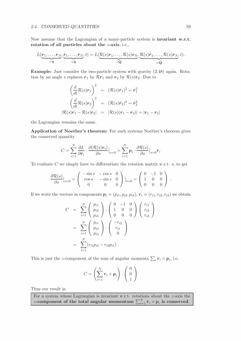
2.4. CONSERVED QUANTITIES 59
Now assume that the Lagrangian of a many-particle system is invariant w.r.t.rotation of all particles about the z-axis, i.e.,
L(r1, . . . , rN︸ ︷︷ ︸
=q
, r1, . . . , rN︸ ︷︷ ︸
=q
, t) = L(R(s)r1, . . . ,R(s)rN︸ ︷︷ ︸
=Q
,R(s)r1, . . . ,R(s)rN︸ ︷︷ ︸
=Q
, t).
Example: Just consider the two-particle system with gravity (2.48) again. Rota-tion by an angle s replaces r1 by Rr1 and r2 by R(s)r2. Due to
(d
dtR(s)r1
)2
= (R(s)r1)2 = r2
1
(d
dtR(s)r2
)2
= (R(s)r2)2 = r2
2
|R(s)r1 −R(s)r2| = |R(s)(r1 − r2)| = |r1 − r2|
the Lagrangian remains the same.
Application of Noether’s theorem: For such systems Noether’s theorem givesthe conserved quantity
C =N∑
i=1
∂L
∂ri· ∂(R(s)ri)
∂s
∣∣s=0
=N∑
i=1
pi ·∂R(s)
∂s
∣∣s=0
ri
To evaluate C we simply have to differentiate the rotation matrix w.r.t. s, to get
∂R(s)
∂s
∣∣s=0
=
− sin s − cos s 0cos s − sin s 0
0 0 0
∣∣s=0
=
0 −1 01 0 00 0 0
.
If we write the vectors in components pi = (pi1, pi2, pi3), ri = (ri1, ri2, ri3) we obtain
C =
N∑
i=1
pi1
pi2
pi3
·
0 −1 01 0 00 0 0
ri1
ri2
ri3
=
N∑
i=1
pi1
pi2
pi3
·
−ri2
ri1
0
=
N∑
i=1
(ri1pi2 − ri2pi1) .
This is just the z-component of the sum of angular momenta∑
i ri × pi, i.e.
C =
(N∑
i=1
ri × pi
)
·
001
Thus our result is:
For a system whose Lagrangian is invariant w.r.t. rotations about the z-axis thez-component of the total angular momentum
∑Ni=1 ri × pi is conserved.
60 CHAPTER 2. LAGRANGIAN MECHANICS
Analogous results hold for the y-axis, the z-axis and all other axes going throughthe origin. Therefore:
For a system whose Lagrangian is invariant w.r.t. rotations about all axis goingthrough the origin we have
N∑
i=1
ri × pi = const.
Summary
Symmetries of the Lagrangian lead to conservation laws:
symmetry w.r.t. conserved quantity
translations total momentumrotations total angular momentum
Even energy conservation can be placed in this context: If the Lagrangian does notdepend on time this means that the system looks the same for all times, i.e., it isinvariant w.r.t. “translations in time”. The resulting conservation law is energyconservation:
symmetry w.r.t. conserved quantity
translations in time (generalised) energy
These symmetries are satisfied by a large class of systems:
Thm: If the Lagrangian of a system depends only
• the squared velocities r2i and
• the distances |ri − rj|
of the particles, then all symmetries and conservation laws above are satisfied, i.e.:
• translation symmetry ⇒ total momentum conservation
• rotation symmetry ⇒ total angular momentum conservation
• independence from t ⇒ (generalised) energy conservation
Proof: (Just generalise what we said about example (2.48).)
• Translation symmetry: The squared velocities ri are invariant under transla-tions as replacing ri by ri + sd doesn’t change the derivative:
(d
dt(ri + sd)
)2
= r2i .
The distances |ri − rj| are translation invariant as
|(ri + sd) − (rj + sd)| = |ri − rj|.
2.4. CONSERVED QUANTITIES 61
• Rotation symmetry: The squared velocities are invariant under rotation, i.e.replacing ri by R(s)ri as
(d
dtR(s)ri
)2
= (R(s)ri)2 = r2
i .
Here we have used that rotation doesn’t change the norm or the square of avector. The distances are invariant under rotation as
|R(s)ri −R(s)rj | = |R(s)(ri − rj)| = |ri − rj |
where we have used the same result about the norm or the square.
• Independence from t: By assumption L does not depend explicitly on time,only through r2
i and |ri − rj |.Note: The total momentum and the total angular momentum each have three com-ponents. The generalised energy is just a real number. Hence there are altogetherseven conserved numbers.
Examples:
• The kinetic energy∑
i mir2i depends only on squared velocities. The same
applies to many common potentials: e.g. the potential energy of a springdepends only on the distance between the endpoints, the potential due togravitational attraction between two particles depends only the distance be-tween the particles.
• Assume that our system is in the gravitational field of the Earth. Thenthe potential will contain terms
− GmimEarth
|ri − rEarth|accounting for the gravitational attraction between each particle i and theEarth. These terms will satisfy the above conditions only if we take Earthas part of our system. Then we have a so-called isolated system wherenone of the particles interacts with anything outside the system, and all ourconservation laws hold.
• Now let’s see which conservation laws if we don’t include Earth in oursystem, and use the approximation migzi for the gravitational potential ofthe i-th particle (while all other terms in the Lagrangian are innocent).
– Translation symmetry: The potential remains invariant if we change allxi and yi by the same amount but not if we change the zi’s. Hence weonly have translation invariance in x- and y-direction, and only the xand y-components of the total momentum are conserved.
– Rotation symmetry: The gravitational potential remains invariant if werotate all particles about the z-axis, as this does not change their z-coordinates. Hence the z-component of the total angular momentum isconserved. However rotations about the x- or the y-axis change the z-coordinates of the particles and thus the gravitational potential. Hencethe corresponding components of the total angular momentum are notconserved.
62 CHAPTER 2. LAGRANGIAN MECHANICS
– Independence from t: The gravitational potential does not depend ex-plicitly on time. Hence the generalised energy is conserved.
We thus have only four conserved numbers.
Chapter 3
Small oscillations
3.1 General theory
We will now study systems performing oscillations close to a minimum of a potential.The prototypical system displaying oscillations is the one-dimensional harmonicoscillator, with a potential energy that is quadratic in the coordinate, and a kineticenergy that is quadratic in the velocity. To generalise this example we investigatesystems with an arbitrary number d of generalised coordinates (collected into avector q = (q1, q2, . . . , qd)) and a Lagrangian of the form:
Generalised harmonic oscillator
L = T − U =1
2q · M q − 1
2q · Kq . (3.1)
Here the potential energy is quadratic in q and kinetic energy is quadratic in q. Mand K are assumed to be constant, real, symmetric matrices of size d×d. Moreover,the matrix M must be positive definite, i.e., for all q 6= 0 we must have q ·M q > 0.This condition is needed because the kinetic energy T = 1
2 q · M q, being the sumof the non-negative kinetic energies of the particles making up our system, must benon-negative as well (usually positive, unless all particles are at rest and we thushave q = 0).
Applications for Lagrangians of the above type are
• systems composed of springs since the potential of a spring is quadratic.
• Much more generally, we will see that close to extrema of the potential(almost) any Lagrangian can be approximated by one of the form (3.1).
Lagrange equation
The Lagrangian (3.1) has the derivatives
∂L
∂q= −Kq
∂L
∂q= M q .
63
64 CHAPTER 3. SMALL OSCILLATIONS
Thus, Lagrange’s equationd
dt
∂L
∂q=
∂L
∂q
boils down to
M q = −Kq (3.2)
This is a linear differential equation, i.e., linear combinations of solutions are alsosolutions.
Normal modes
As for any linear differential equation, it is a good idea to look for particularlysimple solutions, and then write general solutions as a linear combination of thesesimple solutions. Motivated by the example of the harmonic oscillator we thus lookfor solutions of the form
q(t) = u cos(ωt) (3.3)
or
q(t) = u sin(ωt) . (3.4)
These solutions are called normal modes, and ω ∈ C is called the normal fre-quency. If we insert (3.3) and its second derivative
q(t) = −u ω2 cos(ωt)
into Lagrange’s equation (3.2) we obtain
−Mu ω2 cos(ωt) = −Ku cos(ωt) .
The same result would be obtained for Eq. (3.3) with the cosine replaced by a sine.To have these equations satisfied for all t we need
(K − ω2M)u = 0 . (3.5)
This equation is similar to a familiar one: If M were replaced by the unit matrix 1,Eq. (3.5) would turn into the equation for eigenvalues and eigenvectors of a matrixK, (K − ω21)u = 0. Eq. (3.5) thus represents a generalised eigenvalue prob-lem. Accordingly the solutions for ω2 are called the generalised eigenvalues,and the solutions for u are referred to as the generalised eigenvectors.
Now how can we get u and ω?
• First, we have to realise that (K − ω2M)u = 0 has nonzero solutions u onlyif
det(K − ω2M) = 0 . (3.6)
This is because multiplication of a matrix like K−ω2M with a nonzero vectorcan yield a zero result only if the determinant of the matrix is equal to zero.Again (3.6) is analogous to the result known from Linear Algebra for the caseM = 1. Eq. (3.6) is called the characteristic (or secular) equation.det(K − ω2M) is called the characteristic (or secular) polynomial. To
3.1. GENERAL THEORY 65
show that it is a polynomial and determine its degree we use that like anydeterminant of a d × d-matrix
det(K − ω2M) = det
K11 − ω2M11 K12 − ω2M12 . . .K21 − ω2M21 K22 − ω2M22 . . .
......
. . .
can be written as a sum over products of d matrix elements. These matrixelements each involve a term proportional to ω2 and a term independent of ω2.The product of d such matrix elements thus contains terms proportional to1, ω2, ω4, etc., up to ω2d. Hence det(K − ω2M) is a polynomial of degreed in ω2. The solutions for ω2 in det(K − ω2M) = 0, i.e., the generalisedeigenvalues, can now be obtained as roots of the characteristic polynomial.As for any polynomial of degree d there must be d complex roots. These rootswill be denoted by ω2
1, ω22 , . . . ω
2d.
• The generalised eigenvectors u1,u2, . . . ,ud corresponding to ω21 , ω
22, . . . ω
2d are
now obtained as solutions of the equation
(K − ω2j M)uj = 0 . (3.7)
We will focus on the case where all eigenvalues ω2j are different from each other.
Then there is one generalised eigenvector uj for each generalised eigenvalue (up tomultiplication with a complex number).1
If a generalised eigenvalue ω2j is zero, the corresponding normal modes uj cos(ωjt)
and ui sin(ωjt) have to be replaced by uj and ujt. This can be seen as follows:q(t) = uj is a solution because insertion into (3.2) leads to
Md2uj
dt2= −Kuj ⇐⇒ 0 = −Kuj
which is satisfied due to (K −ω21M)uj with ω2
j = 0. Similarly for q(t) = ujt we get
Md2uj
dt2= −Kujt ⇐⇒ 0 = −Kujt .
General solution
The general solution of our equations of motion (3.2) can be written as a linearcombination of the normal modes. If all eigenvalues are different from zero we thusobtain
q(t) =
d∑
j=1
(ajuj cos(ωjt) + bjuj sin(ωjt)) (3.8)
where the constants aj, bj are determined by the initial conditions.
1The characteristic equation may also have multiple roots. For example, if det(K − ω2M) isproportional to (ω2
− 1)3 then ω2 = 1 is a triple root, and three of the eigenvalues, say, ω21 , ω2
2 andω2
3 , coincide. One can show that for an n-fold root, the equation (K − ω2j M)u = 0 has n linearly
independent solutions (proof: see Anton, Elementary Linear Algebra or Lang, Linear Algebra). Inthe above example, we can thus pick linearly independent vectors for u1, u2, and u3 and then theremaining treatment is the same as in the case where all eigenvalues are different.
66 CHAPTER 3. SMALL OSCILLATIONS
Remarks:
1. Which values can ωj take?
First of all, we show that the generalised eigenvalues ω2j are always real.
Proof: Take the generalised eigenvalue equation (3.7) and multiply with thecomplex conjugate of uj, i.e., u∗
j . This gives
u∗j · (K − ω2
j M)uj = 0
and thus
u∗j · Kuj = ω2
j u∗j · Muj ⇒ ω2
j =u∗
j · Kuj
u∗j · Muj
. (3.9)
Here u∗j · Kuj satisfies
(u∗j · Kuj)
∗ = uj · K∗u∗j = uj · Ku∗
j = u∗j · Kuj ;
the second equality sign follows because K is real and the third one followsbecause K is symmetric. u∗
j ·Kuj thus coincides with its complex conjugate,and is a real number. The same applies to u∗
j · Muj . Due to Eq. (3.9) this
means that ω2j is real.
This leaves the following possibilities for ωj:
• ωj can be real and different from zero. Then the normal modes uj cos(ωj)and uj sin(ωjt) describe oscillations. Here the sign of ωj is not impor-tant. Changing the sign only flips the sign of uj sin(ωjt) which can becompensated by also flipping the sign of bj in our general solution (3.8).Hence in the present case ωj can always be taken positive.
• ωj can be purely imaginary and different from zero, i.e. ωj = iρj whereρj is real and different from zero. The normal modes then take the formuj cos(ωjt) = uj cosh(ρjt) and uj sin(ωjt) = uj sinh(ρjt). Alternativelywe can write the solutions as linear combinations of uje
ρjt and uje−ρjt,
i.e., our coordinates increase or decrease exponentially. Similarly asabove ρj can always be taken positive.
• We have already shown that ωj = 0 leads to normal modes constant andlinear in t.
Due to ω2j being real the generalised eigenvalue equation (K −ω2
j M)uj = 0 isa real equation, and the eigenvectors uj can be chosen real as well.
2. Are the eigenvectors orthogonal?
For M = 1, it was shown in Linear Algebra that the eigenvectors correspond-ing to different eigenvalues are orthogonal, i.e., uj · uk = 0 if ω2
j 6= ω2k. For
general M we obtain a generalised orthogonality relation: For ω2j 6= ω2
k
we have uj · Muk = 0.
Proof: We write
(ω2j − ω2
k)uj · Muk = uk · ω2j Muj − uj · ω2
kMuk
= uk · Kuj − uj · Kuk
= 0 .
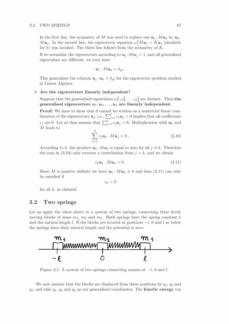
3.2. TWO SPRINGS 67
In the first line, the symmetry of M was used to replace one uj ·Muk by uk ·Muj. In the second line, the eigenvector equation ω2
j Muj = Kuj (similarlyfor k) was invoked. The third line follows from the symmetry of K.
If we normalise the eigenvectors according to uj ·Muj = 1, and all generalisedeigenvalues are different, we even have
uj · Muk = δjk .
This generalises the relation uj ·uk = δjk for the eigenvector problem studiedin Linear Algebra.
3. Are the eigenvectors linearly independent?
Suppose that the generalised eigenvalues ω21, ω
22 , . . . , ω
2d are distinct. Then the
generalised eigenvectors u1,u2, . . . ,ud are linearly independent.
Proof: We have to show that 0 cannot be written as a nontrivial linear com-bination of the eigenvectors uj , i.e.,
∑dj=1 cjuj = 0 implies that all coefficients
cj are 0. Let us thus assume that∑d
j=1 cjuj = 0. Multiplication with uk andM leads to
d∑
j=1
cjuk · Muj = 0 . (3.10)
According to 3. the product uk ·Muj is equal to zero for all j 6= k. Thereforethe sum in (3.10) only receives a contribution from j = k, and we obtain
ckuk · Muk = 0 . (3.11)
Since M is positive definite we have uk · Muk 6= 0 and thus (3.11) can onlybe satisfied if
ck = 0
for all k, as claimed.
3.2 Two springs
Let us apply the ideas above to a system of two springs, connecting three freelymoving blocks of mass m1, m2 and m1. Both springs have the spring constant kand the natural length l. If the blocks are located at positions −l, 0 and l as belowthe springs have their natural length and the potential is zero:
Figure 3.1: A system of two springs connecting masses at −l, 0 and l.
We now assume that the blocks are displaced from these positions by q1, q2 andq3, and take q1, q2 and q3 as our generalised coordinates: The kinetic energy can
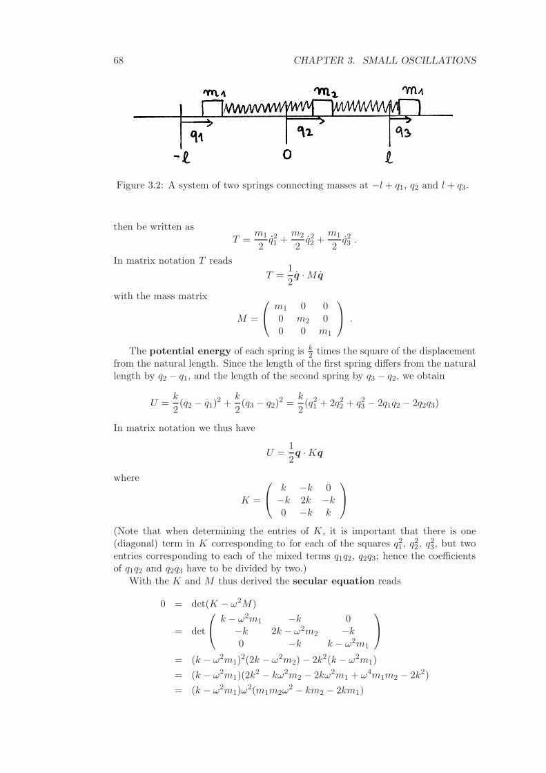
68 CHAPTER 3. SMALL OSCILLATIONS
Figure 3.2: A system of two springs connecting masses at −l + q1, q2 and l + q3.
then be written as
T =m1
2q21 +
m2
2q22 +
m1
2q23 .
In matrix notation T reads
T =1
2q · M q
with the mass matrix
M =
m1 0 00 m2 00 0 m1
.
The potential energy of each spring is k2 times the square of the displacement
from the natural length. Since the length of the first spring differs from the naturallength by q2 − q1, and the length of the second spring by q3 − q2, we obtain
U =k
2(q2 − q1)
2 +k
2(q3 − q2)
2 =k
2(q2
1 + 2q22 + q2
3 − 2q1q2 − 2q2q3)
In matrix notation we thus have
U =1
2q · Kq
where
K =
k −k 0−k 2k −k0 −k k
(Note that when determining the entries of K, it is important that there is one(diagonal) term in K corresponding to for each of the squares q2
1, q22 , q2
3, but twoentries corresponding to each of the mixed terms q1q2, q2q3; hence the coefficientsof q1q2 and q2q3 have to be divided by two.)
With the K and M thus derived the secular equation reads
0 = det(K − ω2M)
= det
k − ω2m1 −k 0−k 2k − ω2m2 −k0 −k k − ω2m1
= (k − ω2m1)2(2k − ω2m2) − 2k2(k − ω2m1)
= (k − ω2m1)(2k2 − kω2m2 − 2kω2m1 + ω4m1m2 − 2k2)
= (k − ω2m1)ω2(m1m2ω
2 − km2 − 2km1)
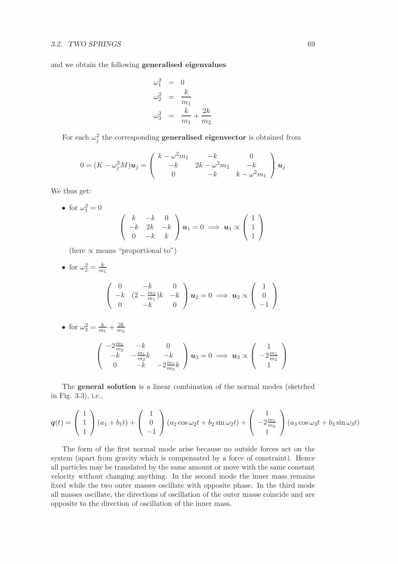
3.2. TWO SPRINGS 69
and we obtain the following generalised eigenvalues
ω21 = 0
ω22 =
k
m1
ω23 =
k
m1+
2k
m2
For each ω2j the corresponding generalised eigenvector is obtained from
0 = (K − ω2j M)uj =
k − ω2m1 −k 0−k 2k − ω2m2 −k0 −k k − ω2m1
uj
We thus get:
• for ω21 = 0
k −k 0−k 2k −k0 −k k
u1 = 0 =⇒ u1 ∝
111
(here ∝ means “proportional to”)
• for ω22 = k
m1
0 −k 0−k (2 − m2
m1)k −k
0 −k 0
u2 = 0 =⇒ u2 ∝
10−1
• for ω23 = k
m1+ 2k
m2
−2m1m2
−k 0
−k −m1m2
k −k
0 −k −2m1m2
k
u3 = 0 =⇒ u3 ∝
1−2m1
m2
1
The general solution is a linear combination of the normal modes (sketchedin Fig. 3.3), i.e.,
q(t) =
111
(a1 + b1t) +
10−1
(a2 cos ω2t + b2 sin ω2t) +
1−2m1
m2
1
(a3 cos ω3t + b3 sin ω3t)
The form of the first normal mode arise because no outside forces act on thesystem (apart from gravity which is compensated by a force of constraint). Henceall particles may be translated by the same amount or move with the same constantvelocity without changing anything. In the second mode the inner mass remainsfixed while the two outer masses oscillate with opposite phase. In the third modeall masses oscillate, the directions of oscillation of the outer masse coincide and areopposite to the direction of oscillation of the inner mass.
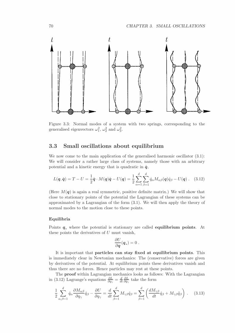
70 CHAPTER 3. SMALL OSCILLATIONS
Figure 3.3: Normal modes of a system with two springs, corresponding to thegeneralised eigenvectors ω2
1, ω22 and ω2
3.
3.3 Small oscillations about equilibrium
We now come to the main application of the generalised harmonic oscillator (3.1):We will consider a rather large class of systems, namely those with an arbitrarypotential and a kinetic energy that is quadratic in q,
L(q, q) = T − U =1
2q · M(q)q − U(q) =
1
2
d∑
α=1
d∑
β=1
qαMαβ(q)qβ − U(q) . (3.12)
(Here M(q) is again a real symmetric, positive definite matrix.) We will show thatclose to stationary points of the potential the Lagrangian of these systems can beapproximated by a Lagrangian of the form (3.1). We will then apply the theory ofnormal modes to the motion close to these points.
Equilibria
Points q∗ where the potential is stationary are called equilibrium points. Atthese points the derivatives of U must vanish,
∂U
∂q(q∗) = 0 .
It is important that particles can stay fixed at equilibrium points. Thisis immediately clear in Newtonian mechanics: The (conservative) forces are givenby derivatives of the potential. At equilibrium points these derivatives vanish andthus there are no forces. Hence particles may rest at these points.
The proof within Lagrangian mechanics looks as follows: With the Lagrangianin (3.12) Lagrange’s equations ∂L
∂qγ= d
dt∂L∂qγ
take the form
1
2
d∑
α,β=1
qα∂Mαβ
∂qγqβ − ∂U
∂qγ=
d
dt
d∑
β=1
Mγβ qβ =
d∑
β=1
(dMγβ
dtqβ + Mγβ qβ
)
. (3.13)
3.3. SMALL OSCILLATIONS ABOUT EQUILIBRIUM 71
This equation is indeed satisfied for q(t) = q∗ = const, since for constant q the timederivatives vanish, and the term ∂U
∂qγvanishes at stationary points of U .
Approximation close to equilibrium
To give an approximation for the Lagrangian L that is valid close to the equilibrium,we write
q(t) = q∗ + δq(t)
which in particular impliesq = δq .
We then make a Taylor expansion up to second order in δq, δq.For the potential this expansion reads
U(q) ≈ U(q∗) +
d∑
α=1
∂U
∂qα(q∗)
︸ ︷︷ ︸
=0
δqα +1
2
d∑
α=1
d∑
β=1
∂2U
∂qα∂qβ(q∗)
︸ ︷︷ ︸
≡Kαβ
δqαδqβ
where ≈ indicates dropping all terms of cubic or higher order. The linear termvanishes due to dU
dqα(q∗) = 0. The quadratic terms can be written in a simple form
if we collect the second derivatives of the potential at the equilibrium point into amatrix K with entries
Kαβ =∂2U
∂qα∂qβ(q∗) .
We then obtain
U(q) ≈ U(q∗) +1
2δq · Kδq (3.14)
For the kinetic energy we write
T =1
2q · M(q)q =
1
2δq · M(q)δq
≈ 1
2δq · (M(q∗) + terms of order δq and higher) δq .
Since we drop wall terms with more than two δq, δq this is approximated by
T ≈ 1
2δq · M(q∗)δq .
In the vicinity of the equilibrium point q∗, the Lagrangian L thus becomes
L = T − U ≈ 1
2δq · M(q∗)δq − U(q∗) −
1
2δq · Kδq (3.15)
This is just the form of the Lagrangian considered in Section (3.1), with δq and δqtaking the place of q and q. The only difference is the constant −U(q∗) whichhowever does not affect the equations of motion.
Example: Imagine a linear molecule with three atoms of mass m1, m2 andm1, and a potential that consists of a complicated term depending on the distancebetween the first and the second atom, and an analogous term depending on thedistance between the second and the third atom. Apart from the form of thepotential this situation is analogous to the system with two springs in Section 3.2
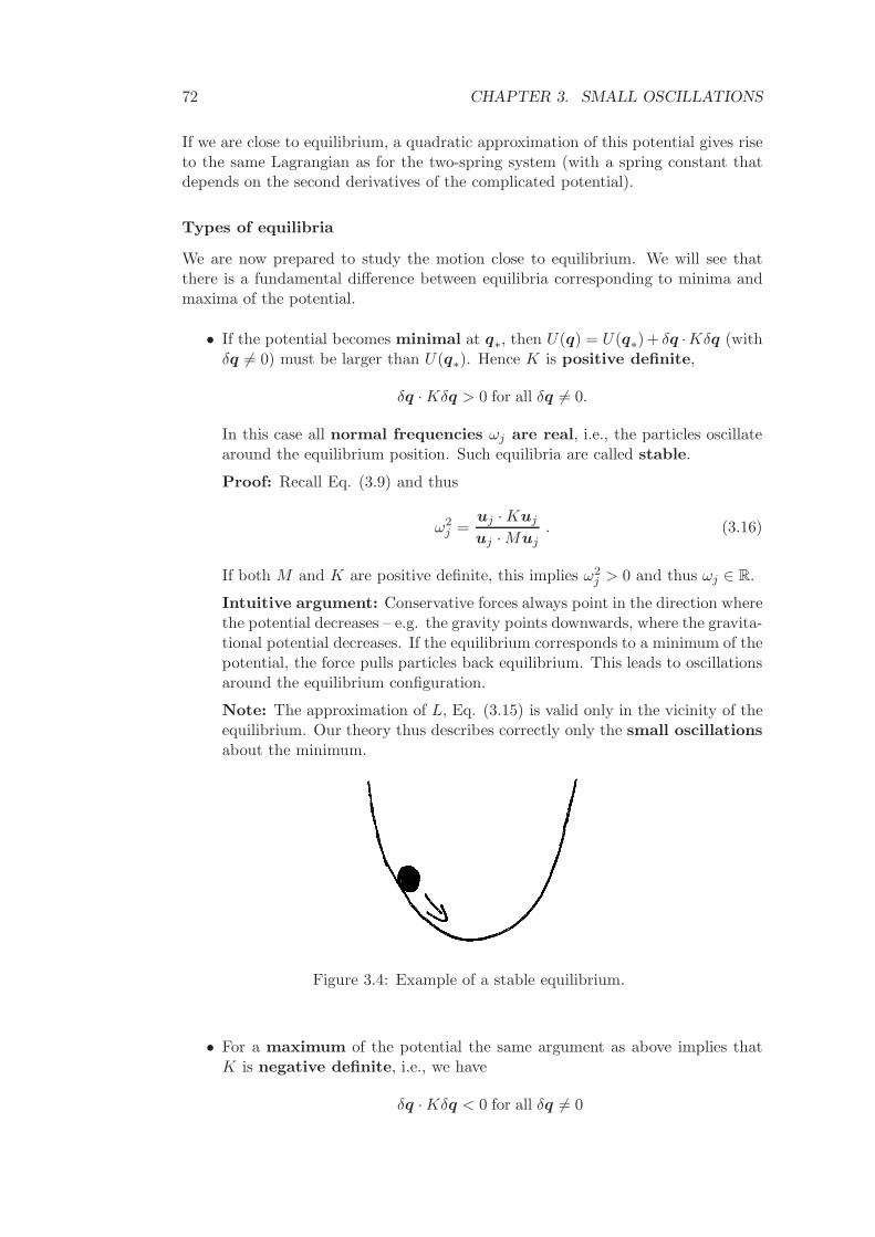
72 CHAPTER 3. SMALL OSCILLATIONS
If we are close to equilibrium, a quadratic approximation of this potential gives riseto the same Lagrangian as for the two-spring system (with a spring constant thatdepends on the second derivatives of the complicated potential).
Types of equilibria
We are now prepared to study the motion close to equilibrium. We will see thatthere is a fundamental difference between equilibria corresponding to minima andmaxima of the potential.
• If the potential becomes minimal at q∗, then U(q) = U(q∗)+ δq ·Kδq (withδq 6= 0) must be larger than U(q∗). Hence K is positive definite,
δq · Kδq > 0 for all δq 6= 0.
In this case all normal frequencies ωj are real, i.e., the particles oscillatearound the equilibrium position. Such equilibria are called stable.
Proof: Recall Eq. (3.9) and thus
ω2j =
uj · Kuj
uj · Muj. (3.16)
If both M and K are positive definite, this implies ω2j > 0 and thus ωj ∈ R.
Intuitive argument: Conservative forces always point in the direction wherethe potential decreases – e.g. the gravity points downwards, where the gravita-tional potential decreases. If the equilibrium corresponds to a minimum of thepotential, the force pulls particles back equilibrium. This leads to oscillationsaround the equilibrium configuration.
Note: The approximation of L, Eq. (3.15) is valid only in the vicinity of theequilibrium. Our theory thus describes correctly only the small oscillationsabout the minimum.
Figure 3.4: Example of a stable equilibrium.
• For a maximum of the potential the same argument as above implies thatK is negative definite, i.e., we have
δq · Kδq < 0 for all δq 6= 0
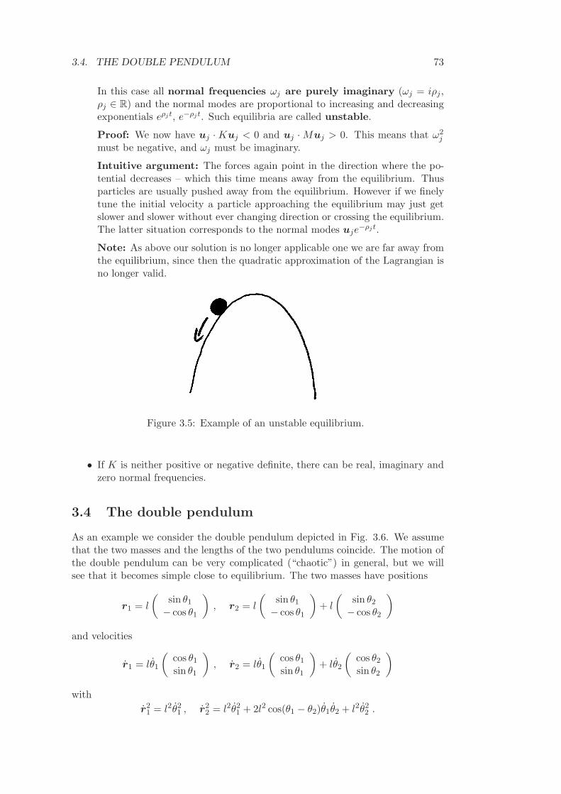
3.4. THE DOUBLE PENDULUM 73
In this case all normal frequencies ωj are purely imaginary (ωj = iρj ,ρj ∈ R) and the normal modes are proportional to increasing and decreasingexponentials eρjt, e−ρjt. Such equilibria are called unstable.
Proof: We now have uj · Kuj < 0 and uj · Muj > 0. This means that ω2j
must be negative, and ωj must be imaginary.
Intuitive argument: The forces again point in the direction where the po-tential decreases – which this time means away from the equilibrium. Thusparticles are usually pushed away from the equilibrium. However if we finelytune the initial velocity a particle approaching the equilibrium may just getslower and slower without ever changing direction or crossing the equilibrium.The latter situation corresponds to the normal modes uje
−ρjt.
Note: As above our solution is no longer applicable one we are far away fromthe equilibrium, since then the quadratic approximation of the Lagrangian isno longer valid.
Figure 3.5: Example of an unstable equilibrium.
• If K is neither positive or negative definite, there can be real, imaginary andzero normal frequencies.
3.4 The double pendulum
As an example we consider the double pendulum depicted in Fig. 3.6. We assumethat the two masses and the lengths of the two pendulums coincide. The motion ofthe double pendulum can be very complicated (“chaotic”) in general, but we willsee that it becomes simple close to equilibrium. The two masses have positions
r1 = l
(sin θ1
− cos θ1
)
, r2 = l
(sin θ1
− cos θ1
)
+ l
(sin θ2
− cos θ2
)
and velocities
r1 = lθ1
(cos θ1
sin θ1
)
, r2 = lθ1
(cos θ1
sin θ1
)
+ lθ2
(cos θ2
sin θ2
)
with
r21 = l2θ2
1 , r22 = l2θ2
1 + 2l2 cos(θ1 − θ2)θ1θ2 + l2θ22 .
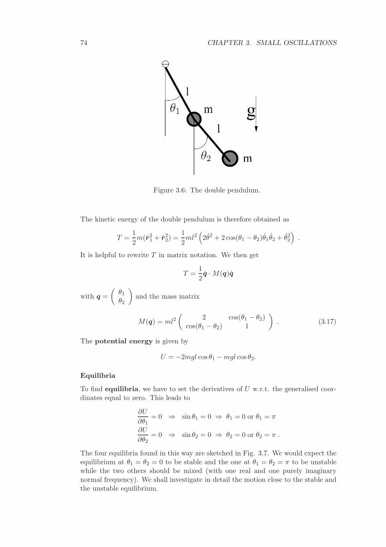
74 CHAPTER 3. SMALL OSCILLATIONS
Figure 3.6: The double pendulum.
The kinetic energy of the double pendulum is therefore obtained as
T =1
2m(r2
1 + r22) =
1
2ml2
(
2θ2 + 2cos(θ1 − θ2)θ1θ2 + θ22
)
.
It is helpful to rewrite T in matrix notation. We then get
T =1
2q · M(q)q
with q =
(θ1
θ2
)
and the mass matrix
M(q) = ml2(
2 cos(θ1 − θ2)cos(θ1 − θ2) 1
)
. (3.17)
The potential energy is given by
U = −2mgl cos θ1 − mgl cos θ2.
Equilibria
To find equilibria, we have to set the derivatives of U w.r.t. the generalised coor-dinates equal to zero. This leads to
∂U
∂θ1= 0 ⇒ sin θ1 = 0 ⇒ θ1 = 0 or θ1 = π
∂U
∂θ2= 0 ⇒ sin θ2 = 0 ⇒ θ2 = 0 or θ2 = π .
The four equilibria found in this way are sketched in Fig. 3.7. We would expect theequilibrium at θ1 = θ2 = 0 to be stable and the one at θ1 = θ2 = π to be unstablewhile the two others should be mixed (with one real and one purely imaginarynormal frequency). We shall investigate in detail the motion close to the stable andthe unstable equilibrium.
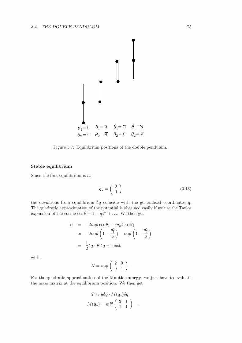
3.4. THE DOUBLE PENDULUM 75
Figure 3.7: Equilibrium positions of the double pendulum.
Stable equilibrium
Since the first equilibrium is at
q∗ =
(00
)
(3.18)
the deviations from equilibrium δq coincide with the generalised coordinates q.The quadratic approximation of the potential is obtained easily if we use the Taylorexpansion of the cosine cos θ = 1 − 1
2θ2 + . . .. We then get
U = −2mgl cos θ1 − mgl cos θ2
≈ −2mgl
(
1 − θ21
2
)
− mgl
(
1 − θ22
2
)
=1
2δq · Kδq + const
with
K = mgl
(2 00 1
)
.
For the quadratic approximation of the kinetic energy, we just have to evaluatethe mass matrix at the equilibrium position. We then get
T ≈ 12δq · M(q∗)δq
M(q∗) = ml2(
2 11 1
)
.
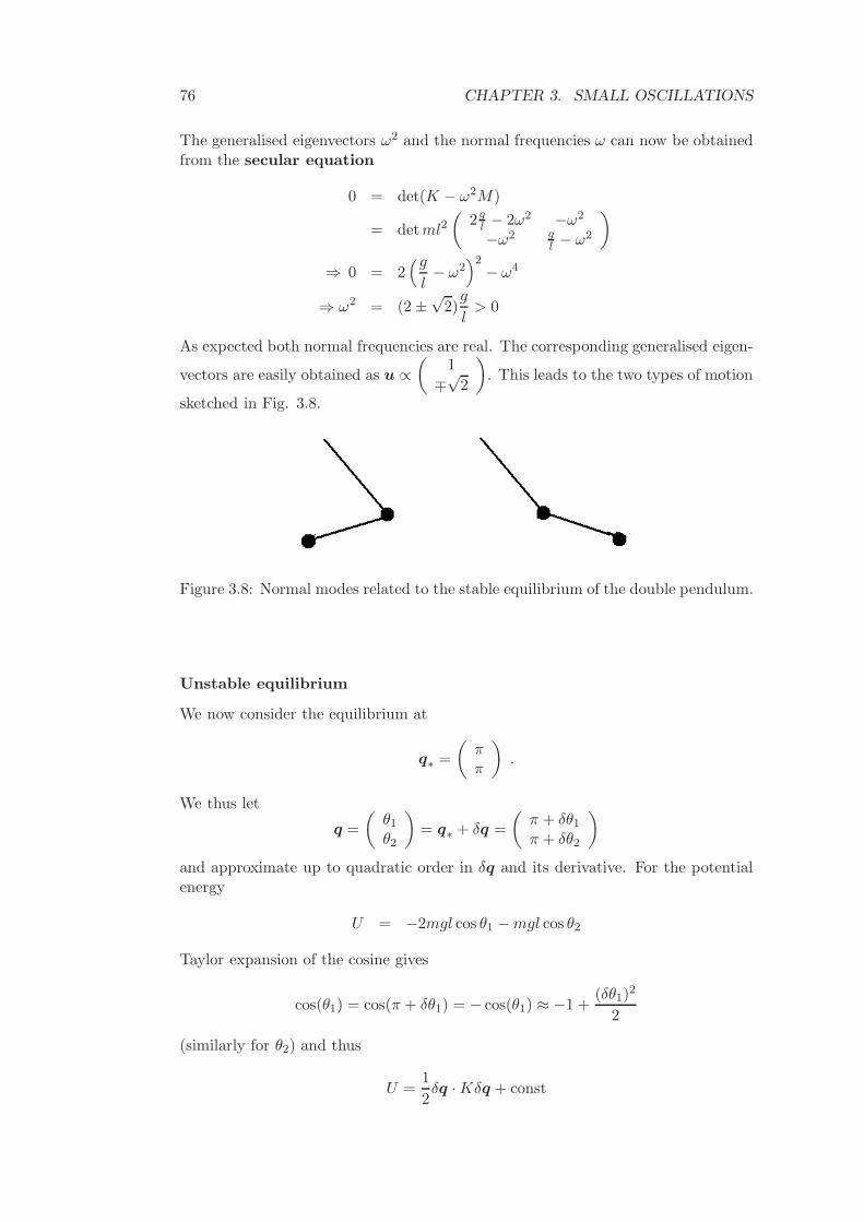
76 CHAPTER 3. SMALL OSCILLATIONS
The generalised eigenvectors ω2 and the normal frequencies ω can now be obtainedfrom the secular equation
0 = det(K − ω2M)
= detml2(
2gl − 2ω2 −ω2
−ω2 gl − ω2
)
⇒ 0 = 2(g
l− ω2
)2− ω4
⇒ ω2 = (2 ±√
2)g
l> 0
As expected both normal frequencies are real. The corresponding generalised eigen-
vectors are easily obtained as u ∝(
1
∓√
2
)
. This leads to the two types of motion
sketched in Fig. 3.8.
Figure 3.8: Normal modes related to the stable equilibrium of the double pendulum.
Unstable equilibrium
We now consider the equilibrium at
q∗ =
(ππ
)
.
We thus let
q =
(θ1
θ2
)
= q∗ + δq =
(π + δθ1
π + δθ2
)
and approximate up to quadratic order in δq and its derivative. For the potentialenergy
U = −2mgl cos θ1 − mgl cos θ2
Taylor expansion of the cosine gives
cos(θ1) = cos(π + δθ1) = − cos(θ1) ≈ −1 +(δθ1)
2
2
(similarly for θ2) and thus
U =1
2δq · Kδq + const
3.4. THE DOUBLE PENDULUM 77
with
K = −mgl
(2 00 1
)
.
The kinetic energy is approximated by
T ≈ 1
2δq · M(q∗)δq
where the mass matrix at equilibrium again reads
M(q∗) = ml2(
2 11 1
)
.
Compared to the stable equilibrium, only K has changed sign. Since K is pro-portional to g we can thus copy the results from the stable equilibrium with thereplacement g → −g. This yields
ω2 = −(2 ±√
2)g
l< 0
(i.e. we indeed have two imaginary frequencies) while the generalised eigenvectors
u ∝(
1
∓√
2
)
remain the same.
78 CHAPTER 3. SMALL OSCILLATIONS
Chapter 4
Rigid bodies
An important application of mechanics is the motion of rigid bodies. Rigid bodiesare formally defined as follows:
A rigid body is a system in which the distances between the particles do notvary in time.
Most solid objects around us are rigid bodies to a reasonable approximation,because the distances between the atoms do not vary in time. The distances of theparticles being fixed, there are only few things that one can do with a rigid body:translate it (i.e. move all particles by the same amount in the same direction) androtate it about an arbitrary axis.
In this lecture we will only be interested in rotations about axes throughthe origin. These rotations are important in the following two cases:
• If the body is fixed at the origin, we can no longer move all particles bythe same amount in the same direction. And if we want to rotate the bodywe must make sure that the origin remains fixed. This means that the axis ofrotation must go through the origin.
• Now let us consider a rigid body on which no outside forces are acting, e.g.a rigid body in space. In this case it is helpful to study the motion of thecentre of mass, defined by
N∑
i=1
mi
Mri
where M =∑N
i=1 mi is the overall mass of the system. As any isolated system,such a rigid body satisfies several conservation laws (see Section 2.4.4). Inparticular the overall momentum of all particles is conserved,
N∑
i=1
miri = const .
This implies that
d
dt
N∑
i=1
mi
Mri = const ,
i.e., the velocity of the centre of mass is constant.
79
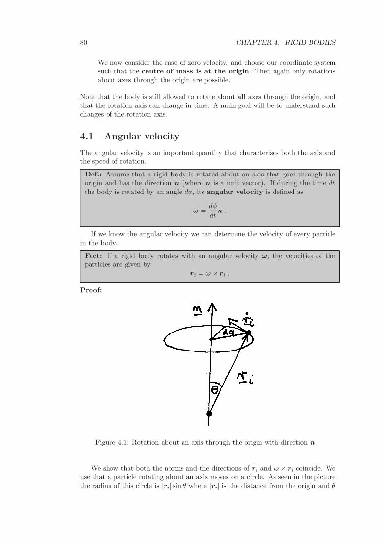
80 CHAPTER 4. RIGID BODIES
We now consider the case of zero velocity, and choose our coordinate systemsuch that the centre of mass is at the origin. Then again only rotationsabout axes through the origin are possible.
Note that the body is still allowed to rotate about all axes through the origin, andthat the rotation axis can change in time. A main goal will be to understand suchchanges of the rotation axis.
4.1 Angular velocity
The angular velocity is an important quantity that characterises both the axis andthe speed of rotation.
Def.: Assume that a rigid body is rotated about an axis that goes through theorigin and has the direction n (where n is a unit vector). If during the time dtthe body is rotated by an angle dφ, its angular velocity is defined as
ω =dφ
dtn .
If we know the angular velocity we can determine the velocity of every particlein the body.
Fact: If a rigid body rotates with an angular velocity ω, the velocities of theparticles are given by
ri = ω × ri .
Proof:
Figure 4.1: Rotation about an axis through the origin with direction n.
We show that both the norms and the directions of ri and ω × ri coincide. Weuse that a particle rotating about an axis moves on a circle. As seen in the picturethe radius of this circle is |ri| sin θ where |ri| is the distance from the origin and θ
4.2. INERTIA TENSOR 81
is the angle enclosed between the position vector and the direction of the axis. Theproduct |ri| sin θ can also be written as |n × ri| (using that n is normalised). Aparticle moved by an angle dφ now travels a distance |n × ri|dφ on the circle. Theabsolute value of its velocity is obtained by dividing out dt. We then get
∣∣ri| = |ndφ
dt︸︷︷︸
=ω
×ri
∣∣ , (4.1)
as desired.
Now we consider the direction of the vectors. The circle that our particle moveson is in a plane perpendicular to the rotation axis, which means that the velocityis perpendicular to n. In addition it is clear from the picture that the velocity isperpendicular to ri. The same holds true for the cross product n × ri. Hence alsothe directions coincide and the statement is proven.
4.2 Inertia tensor
Analogies
It would be nice if we could describe the rotation of rigid bodies in a way analogousto to a motion that we already know very well: the translational motion of a singleparticle. The most important properties of such a particle are its momentum p,its velocity v and its mass m. These quantities are related by p = mv. For arigid body, the analogue of the momentum is the total angular momentum, and theanalogue of the velocity is the angular velocity. The question is therefore: Is therean analogue of the mass as well, and can we use this to write an equation similarto p = mv?
We will see that an analogue of the mass indeed exists; however it is not a reallynumber but a matrix – the so-called inertia tensor. To find it we write the totalangular momentum as
l =
N∑
i=1
ri × pi
=N∑
i=1
ri × miri
=
N∑
i=1
ri × mi(ω × ri)
=N∑
i=1
miri × (ω × ri) . (4.2)
Reassuringly, Eq. (4.2) already expresses the total angular momentum as a linearfunction of the angular velocity. To bring it closer to the form p = mv we use thefollowing formula for combinations of two cross products:
a × (b × c) = b(a · c) − c(a · b)
82 CHAPTER 4. RIGID BODIES
(the so-called “back-cab formula”). We then obtain
l =
N∑
i=1
mi ω(ri · ri) − ri(ri · ω) .
It is now helpful to write out the ath component of the total angular momentum.Since the ri · ri in the first term and the ri · ω in the second term are just realnumbers, for the ath component we have to replace the ω in the first term by ωa
a and the ri in the second term by ria. Writing out the scalar products we thusobtain
la =N∑
i=1
mi
ωa
3∑
c=1
r2ic − ria
3∑
b=1
ribωb
To let the formula look more symmetric, it would be helpful to introduce a sum-mation over b not only in the second term, but also in the first one. We thuswrite
ωa =3∑
b=1
δabωb
with the Kronecker delta already used in Section 2.4.1. If we now pull the sum overb in front of all other terms and shift ωb to the end, we can write the ath componentof the angular momentum as
la =3∑
b=1
N∑
i=1
mi
δab
3∑
c=1
r2ic − riarib
ωb .
We thus obtain the following result:
The total angular momentum l and the angular velocity ω are related by
la =
3∑
b=1
Iabωb
where
Iab =
N∑
i=1
mi
δab
3∑
c=1
r2ic − riarib
.
In matrix notation we havel = Iω
where
I =
I11 I12 I13
I21 I22 I23
I31 I32 I33
is called the inertia tensor.
Rotating coordinate system
The inertia tensor I defined above depends on the coordinates ria which themselvesare functions of time. This can be avoided if we write our vectors in a basis thatdepends on time:
4.2. INERTIA TENSOR 83
In the following, we will use basis vectors E1(t), E2(t),E3(t) that depend on timeand rotate in the same way as the particle positions in the rigid body. This basisis chosen to be orthonormal, i.e., we have
EA(t) · EB(t) = δAB . (4.3)
Moreover we want to have a “right-handed” basis, which means that
E1(t) × E2(t) = E3(t), E2(t) × E3(t) = E1(t),E3(t) × E1(t) = E2(t) . (4.4)
Example: If the body rotates about the z-axis with angular velocity ω =
00ω
we can use
E1(t) =
cos ωtsinωt
0
, E2(t) =
− sin ωtcos ωt
0
, E3(t) =
001
.
Expansion in the new basis: All vectors v(t) can now be expanded in thebasis E1(t),E2(t),E3(t) and the coefficients will be denoted by capital letters,
v(t) =
3∑
A=1
VA(t)EA(t)
For instance we will have
ri(t) =
3∑
A=1
RiAEA(t)
ω(t) =
3∑
A=1
ΩA(t)EA(t)
l(t) =3∑
A=1
LA(t)EA(t) .
Note that here the new particle coordinates RiA don’t depend on time, becausethe basis vectors are rotated in the same way as the particles and the whole timedependence of ri(t) is now in the rotation of the basis vectors EA(t). That’s thereason why we introduced these basis vectors in the first place. We don’t know yethow the total angular momentum and the angular velocity are going to depend ontime, so in contrast to RiA the new coordinates of these quantities still have to bewritten as functions of t.
Due to Eq. (4.3) all scalar products of vectors can be written as sums overproducts of their components in the new basis:
v(t) · w(t) =∑
A
VA(t)EA(t) ·∑
B
WB(t)EB(t)
=∑
A
∑
B
VA(t)WB(t)δAB
=∑
A
VA(t)WA(t) .
84 CHAPTER 4. RIGID BODIES
For scalar products with basis vectors this imples
v(t) · EA(t) = VA(t) .
To apply these ideas to Eq. (4.2) we multiply with EA(t). Repeated applicationof the formula for the scalar product and manipulations similar to the previouscalculation give
LA(t) = l(t) · EA(t)
=
N∑
i=1
mi
[(ω(t) · EA(t))(ri(t) · ri(t)) − (ri(t) · EA(t))(ri(t) · ω(t))
]
=N∑
i=1
mi
[ΩA(t)︸ ︷︷ ︸
=P
B δABΩB(t)
∑
C
R2iC − RiA
∑
B
RiBΩB
]
=∑
B
[N∑
i=1
mi
(
δAB
∑
C
R2iC − RiARiB
)]
︸ ︷︷ ︸
≡IAB
ΩB(t)
=∑
B
IABΩB(t) .
Here IAB is independent of time, like the mass in p = mr! In many cases IAB canbe made diagonal by choosing a convenient set of rotating vectors. The diagonalelements obtained in this way (i.e. the eigenvalues of I are also called momentsof inertia.
Continuously distributed mass
Typically a rigid body contains lots of particles (atoms). In this case a furtherimprovement is very helpful. Instead of summing over all positions Ri of atoms, weassume that the mass is distributed continuously over the rigid body. It is helpfulto describe this distribution in terms of the mass density:
Def.: The mass density ρ(R1, R2, R3) of a rigid body is defined such that themass in a volume from R1 to R1 + dR1, from R2 to R2 + dR2, and form R3 toR3 + dR3 is given by ρ(R1, R2, R3)dR1dR2dR3.
Typically, the mass is just distributed uniformly over the rigid body. Then themass density is simply the overall mass of the body divided by the overall volume.
The elements of the inertia tensor can now be determined as by
IAB =
∫ ∫ ∫
ρ(R1, R2, R3)
(
δAB
∑
C
R2C − RARB
)
dR1dR2dR3 (4.5)
Proof: The contribution of the volume from R1 to R1 + dR1, from R2 toR2 + dR2, and from R3 to R3 + dR3 to IAB is given by
ρ(R1, R2, R3)dR1dR2dR3
(
δAB
∑
C
R2C − RARB
)
.
Integration over the whole body gives Eq. (4.5).
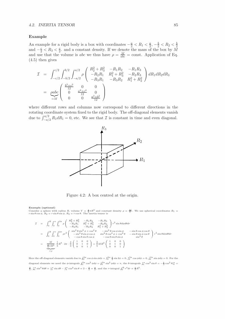
4.2. INERTIA TENSOR 85
Example
An example for a rigid body is a box with coordinates −a2 < R1 < a
2 , − b2 < R2 < b
2and − c
2 < R3 < c2 . and a constant density. If we denote the mass of the box by M
and use that the volume is abc we thus have ρ = Mabc = const. Application of Eq.
(4.5) then gives
I =
∫ c/2
−c/2
∫ b/2
−b/2
∫ a/2
−a/2ρ
R22 + R2
3 −R1R2 −R1R3
−R2R1 R21 + R2
3 −R2R3
−R3R1 −R3R2 R21 + R2
2
dR1dR2dR3
= ρabc︸︷︷︸
=M
b2+c2
12 0 0
0 a2+c2
12 0
0 0 a2+b2
12
where different rows and columns now correspond to different directions in therotating coordinate system fixed to the rigid body. The off-diagonal elements vanish
due to∫ a/2−a/2 R1dR1 = 0, etc. We see that I is constant in time and even diagonal.
Figure 4.2: A box centred at the origin.
Example (optional)
Consider a sphere with radius R, volume V = 4
3πR3 and constant density ρ = M
V. We use spherical coordinates R1 =
r sin θ cos φ, R2 = r sin θ sin φ, R3 = r cos θ. The inertia tensor is
I =
ZR
0
Zπ
0
Z2π
0
ρ
0 R2
2+ R2
3−R1R2 −R1R3
−R2R1 R2
1+ R2
3−R2R3
−R3R1 −R3R2 R2
1+ R2
2
1A r2
sin θdφdθdr
=
ZR
0
Zπ
0
Z2π
0
ρr2
0 sin2 θ sin2 φ + cos2 θ − sin2 θ cos φ sin φ − sin θ cos φ cos θ
− sin2 θ sin φ cos φ sin2 θ cos2 φ + cos2 θ − sin θ sin φ cos θ
− cos θ sin θ cos φ − cos θ sin θ sin φ sin2 θ
1A r2
sin θdφdθdr
=M
4
3πR3| z =ρ
·1
5R
5· 2π ·
4
3
0 1 0 00 1 00 0 1
1A =2
5MR
2
0 1 0 00 1 00 0 1
1AHere the off-diagonal elements vanish due to
R2π0
cos φ sin φdφ =R2π0
1
2sin 2φ = 0,
R2π0
cos φdφ = 0,R2π0
sin φdφ = 0. For the
diagonal elements we need the φ-integralsR2π0
cos2 φdφ =R2π0
sin2 φdφ = π, the θ-integralsR
π0
cos2 sin θ = − 1
3cos2 θ|π
0=
2
3,R
π0
sin3 θdθ =R
π0
sin dθ −R
π0
cos2 sin θ = 2 − 2
3= 4
3, and the r-integral
RR0
r4dr = 1
5R5.
86 CHAPTER 4. RIGID BODIES
4.3 Euler’s equations
We now want to find out how for a rigid body the angular velocity componentsΩ1(t),Ω2(t),Ω3(t) (and thus the axis and speed of rotation) change in time. Forsimplicity we only consider rigid bodies on which no external forces are acting. Thenwe use that for such isolated systems the total angular momentum l is a conservedquantity. We thus obtain
0 =d
dtl
=d
dt
∑
A
LA(t)EA(t)
= L1(t)E1(t) + L2(t)E2(t) + L3(t)E3(t) + L1(t)E1(t) + L2(t)E2(t) + L3(t)E3(t) .
(4.6)
(Note that the conservation of l does not imply conservation of L1(t), L2(t) andL3(t)!) We now need the derivatives of the basis vectors E1(t), E2(t), E3(t). Sincethese basis vectors are rotated in the same way as the particle positions their timederivatives are also obtained by taking a cross product with ω(t). This gives
E1(t) = ω(t) × E1(t)
= (Ω1E1(t) + Ω2(t)E2(t) + Ω3(t)E3(t)) × E1(t)
= −Ω2(t)E3(t) + Ω3(t)E2(t)
where in the second line ω(t) was expanded in terms of the rotating basis vectorsand in the third line I used that we have a right-handed coordinate system (Eq.(4.4)) and that the cross product E1(t) × E1(t) is zero. Analogous reasoning forthe other basis vectors gives
E2(t) = Ω1(t)E3(t) − Ω3(t)E1(t)
E3(t) = −Ω1(t)E2(t) + Ω2(t)E1(t) .
If we sustitute all this into Eq. (4.6) and collect the terms proportional to each ofthe basis vectors we get
L1(t) + Ω2(t)L3(t) − Ω3(t)L2(t) = 0
L2(t) + Ω3(t)L1(t) − Ω1(t)L3(t) = 0
L3(t) + Ω1(t)L2(t) − Ω2(t)L1(t) = 0 . (4.7)
Now we can eliminate the LA(t)’s using that LA(t) =∑
B IABΩB(t). If we chooseour rotating basis in such a way that I becomes diagonal (with diagonal elementsI1, I2 and I3), this relation turns into
LA(t) = IAΩA(t) .
This implies
LA(t) = IAΩA(t) .
Eq. (4.7) thus turns into
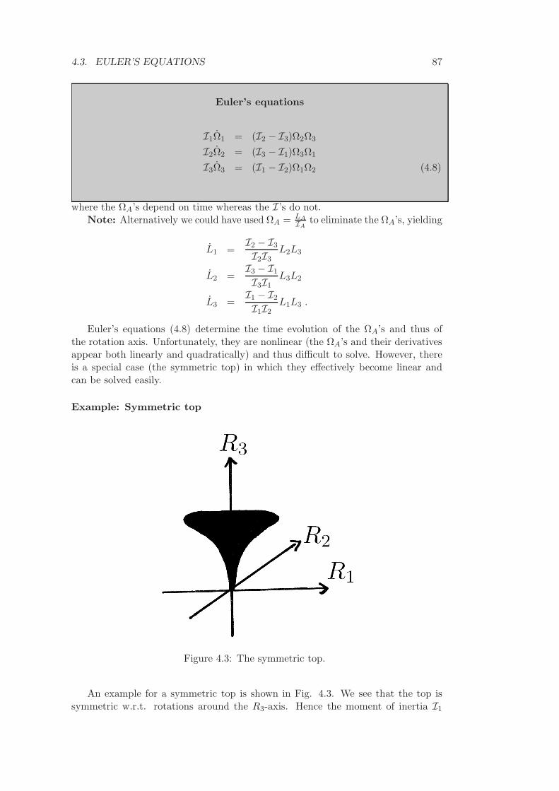
4.3. EULER’S EQUATIONS 87
Euler’s equations
I1Ω1 = (I2 − I3)Ω2Ω3
I2Ω2 = (I3 − I1)Ω3Ω1
I3Ω3 = (I1 − I2)Ω1Ω2 (4.8)
where the ΩA’s depend on time whereas the I’s do not.Note: Alternatively we could have used ΩA = LA
IAto eliminate the ΩA’s, yielding
L1 =I2 − I3
I2I3L2L3
L2 =I3 − I1
I3I1L3L2
L3 =I1 − I2
I1I2L1L3 .
Euler’s equations (4.8) determine the time evolution of the ΩA’s and thus ofthe rotation axis. Unfortunately, they are nonlinear (the ΩA’s and their derivativesappear both linearly and quadratically) and thus difficult to solve. However, thereis a special case (the symmetric top) in which they effectively become linear andcan be solved easily.
Example: Symmetric top
Figure 4.3: The symmetric top.
An example for a symmetric top is shown in Fig. 4.3. We see that the top issymmetric w.r.t. rotations around the R3-axis. Hence the moment of inertia I1
88 CHAPTER 4. RIGID BODIES
corresponding to the R1-axis and the moment of inertia I2 corresponding to theR2-axis should coincide, but differ from the moment of inertia I3 corresponding torotations around the R3-axis. Denoting the two different moments of inertia by I⊥and I‖, we thus have
I1 = I2 = I⊥ 6= I3 = I‖ .
If we insert these momenta into Euler’s equations (4.8), we find
I⊥Ω1 = (I⊥ − I‖)Ω2Ω3
I⊥Ω2 = (I‖ − I⊥)Ω3Ω1
I‖Ω3 = 0 (4.9)
Crucially, the third line implies that the time derivative of Ω3 vanishes. Hence Ω3
(the component of the angular velocity corresponding to rotations around the Z-axis) is a constant. The only thing we still have to do is to solve for Ω1 and Ω2. –This is now a simple task since the first two equations are linear in Ω1 and Ω2. Toproceed we collect the constants I‖, I⊥ and Ω3 into one, denoted by
ν =I⊥ − I‖
I⊥Ω3 = const.
The first two equations in (4.9) thus turn into
Ω1 = −νΩ2 (4.10)
Ω2 = νΩ1 (4.11)
These equations can now easily be solved. If we take the derivative of (4.10) andinsert (4.11) we get
Ω1 = −νΩ2 = −ν2Ω1 .
This is the well-known equation of a harmonic oscillator. The solution reads
Ω1 = C cos(νt + φ) ,
where C and φ are constants that have to be chosen to satisfy the initial conditions.Ω2 can now be determined from Eq. (4.10) as
Ω2 = −1
νΩ1 = C sin(νt + φ)
These equations just indicate a rotation about the R3-axis with frequency ν. Wethus see that the rotation axis of a symmetric top is not fixed (even in a coordinatesystem following the rigid body), but precedes about the R3-axis.
Example: Rotation axis of the Earth
Another example for a rigid body is the Earth. Of course, the Earth has an almostspherical shape. But it is not quite a sphere – the radius of the Equator is a littlebit larger than the distance between the Equator plane and the North pole. Hence,just like for the symmetric top the moments of inertia corresponding to the R1-andR2-direction coincide with each other, but differ slightly from the moment of inertia
4.3. EULER’S EQUATIONS 89
corresponding to the R3-axis. Therefore, Leonhard Euler courageously applied tothe Earth the same results as for the symmetric top. For the Earth we have
I‖ − I⊥I⊥
≈ 1
305
and (since it rotates around itself once in a day)
Ω3 =2π
1 day.
One would thus conclude that the Earth’s rotation axis rotates (precedes) relativeto the surface of the Earth with a frequency
ν =2π
305 days,
i.e., with a period of 305 days. Measurements by Set Carlo Chandler (1846-1913)confirmed the existence of this precession (which is now also called the Chandlerwobble), but he got a period of 433 days! This discrepancy was explained by SimonNewcomb (1835-1909) as being due to the slight non-rigidity of the Earth. Actuallythe Earth is quite rigid, slightly more rigid than steel – but the difference from aperfect rigid body is comparable to the difference of the shape of the Earth from aperfect sphere, which was causing the effect in the first place. It is not possible tokeep into account one of these small effects and neglect the other.

90 CHAPTER 4. RIGID BODIES
Chapter 5
Hamiltonian mechanics
5.1 Hamilton’s equations
Hamiltonian mechanics is a formulation of mechanics similar to the one by Lagrange,but with important advantages. To motivate it, let us recall some results from theprevious chapters.
Reminder
We started from Newtonian mechanics, in particular from Newton’s second lawF = ma. We then derived Lagrange’s formulation of mechanics. The main advan-tage of Lagrange’s formalism is that it looks the same for all coordinate systems, andone can easily account for constraints. The central object in Lagrangian mechanicsis the Lagrangian L(q, q, t) = T −U , depending on the generalised coordinates q,their derivatives q and time t. The trajectories of particles are then obtained fromLagrange’s equations. To solve Lagrange’s equations it is very helpful to identifyconserved quantities of the system. These conserved quantities can be read offfrom the Lagrangian:
• If the Lagrangian is independent of time the generalised energy
h(q, q, t) =∂L
∂q· q − L(q, q, t)
is conserved.
• If the Lagrangian is independent of one of the coordinates qα, the correspond-ing generalised momentum
pα =∂L
∂qα(5.1)
is conserved.
Hamilton
Even though conservation laws can be used in Lagrangian mechanics, the fundamen-tal quantities in Lagrangian mechanics are still the Lagrangian L, the coordinatesq and their derivatives q, not the (potentially) conserved quantities h and p. Thetreatment of conservation laws would be much cleaner if instead we could build
91
92 CHAPTER 5. HAMILTONIAN MECHANICS
the whole theory around h and p. We would thus replace the Lagrangian asthe main quantity of interest by the generalised energy, and use the momenta p
instead of the derivatives q. This is the idea of Hamiltonian mechanics.To replace q one can use that p is determined by q, q and t through (5.1)
p =∂L
∂q= p(q, q, t) . (5.2)
We now assume that this equation can be solved uniquely for q. – This uniquenessis a condition for the applicability of Hamiltonian mechanics. Then q can be writtenas a function of q, p and t,
q = q(q,p, t) . (5.3)
We now want to build a theory based on the generalised energy h. But insteadof writing h as a function of q, q and t we want to replace q as an argument by themomentum p. This can be done if we substitute all occurrences of q by q(q,p, t)and replace ∂L
∂qby p. The resulting function is called the Hamiltonian.
Hamiltonian
H(q,p, t) = h(q, q(q,p, t), t) = p · q(q,p, t) − L(q, q(q,p, t), t)
The Hamiltonian can be used to get equations of motion similar to Lagrange’sequations. These equations have the following form:
Hamilton’s equations
qα =∂H
∂pα
pα = −∂H
∂qα(5.4)
Proof: To prove Hamilton’s equations we compute the partial derivatives of theHamiltonian. There are three terms in H that depend on H: the initial p and twofunctions q(q,p, t). Taking into account all these terms we obtain the derivative∂H∂pα
as
∂H
∂pα= qα + p · ∂q
∂pα− ∂L
∂q︸︷︷︸
=p
· ∂q
∂pα= qα
Here the second and third term cancel due to p = ∂L∂q
. The first equation in (5.4) isthus proven.
To compute ∂H∂qα
we take into account the q-dependence of the two q(q,p, t)’sand of the explicit dependence of L on q. We thus get
∂H
∂qα= p · ∂q
∂qα− ∂L
∂qα− ∂L
∂q︸︷︷︸
=p
· ∂q
∂qα= − ∂L
∂qα
5.1. HAMILTON’S EQUATIONS 93
where again two terms have cancelled. If we now use Lagrange’s equation ∂L∂qα
=ddt
∂L∂qα
and the definition of the momentum we can write the result as
∂H
∂qα= − d
dt
∂L
∂qα︸︷︷︸
=pα
= −pα ,
proving second equation of (5.4).
A related result concerns the time derivative of the Hamiltonian:
∂H
∂t= −∂L
∂t
Proof: Differentiating w.r.t. all three occurrences of t and again using thedefinition of p we get
∂H
∂t= p · ∂q
∂t− ∂L
∂q︸︷︷︸
=p
·∂q
∂t− ∂L
∂t= −∂L
∂t
Examples:
a) Particle in 1d
A particle of mass m in moving in one dimension has the Lagrangian
L =1
2mq2 − U(q)
where U(q) is the potential. The generalised momentum is obtained as
p =∂L
∂q= mq , (5.5)
i.e., it is simply the linear momentum (mass times velocity). Eq. (5.5) can be solvedfor q,
q =p
m. (5.6)
The Hamiltonian is now obtained as
H(q, p, t) = pq − L
where all q’s have to be replaced by pm . We thus get
H(q, p, t) =p2
m−(
p2
2m− U(q)
)
=p2
2m+ U(q) ,
and Hamilton’s equations read
q =∂H
∂p=
p
m(5.7)
p = −∂H
∂q= −∂U
∂q. (5.8)
94 CHAPTER 5. HAMILTONIAN MECHANICS
Here (5.7) is equivalent to the definition of p (see Eq. (5.6)); hence this equationmerely provides a consistency check, whereas (5.8) gives something new. We alsonote that Eqs. (5.7) and (5.8) could be combined into
q =p
m= − 1
m
∂U
∂q. (5.9)
Since −∂U∂q is the conservative force corresponding to the potential U(q), Eq. (5.9)
coincides with Newton’s second law.
b) Particle in 2d, polar coordinates
The Lagrangian of a particle in two dimensions can be written in polar coordinatesρ, φ as
L =1
2mρ2 +
1
2mρ2φ2 − U(ρ, φ) .
We can now determine the momenta associated to ρ and φ and solve for ρ and φ,
pρ =∂L
∂ρ= mρ =⇒ ρ =
pρ
m
pφ =∂L
∂φ= mρ2φ =⇒ φ =
pφ
mρ2.
The Hamiltonian is thus given by
H(ρ, φ, pρ, pφ, t) = pρρ + pφφ − L
=p2
ρ
m+
p2φ
mρ2−(
p2ρ
2m+
p2φ
2mρ2− U(ρ, φ)
)
=p2
ρ
2m+
p2φ
2mρ2+ U(ρ, φ) ,
and Hamilton’s equations read
ρ =∂H
∂pρ=
pρ
m
φ =∂H
∂pφ=
pφ
mρ2
pρ = −∂H
∂ρ=
p2φ
mρ3− ∂U
∂ρ
pφ = −∂H
∂φ= −∂U
∂φ.
Here the first two equations again provide a consistency check with the definitions ofpρ and pφ. The third and fourth equation give the time derivative of the momenta.Again these time derivatives involve partial derivatives of the potential.
Finally we mention that for a central field (a potential U that depends only onρ and thus satisfies ∂U
∂φ = 0) the angular momentum pφ is a conserved quantity (i.e.
φ = 0). In the context of Lagrangian mechanics this was already seen in Section2.4.2.
5.1. HAMILTON’S EQUATIONS 95
c) Quadratic kinetic energy
In the two previous examples the Hamiltonian coincided with the energy E = T +U ,written as a function of q, p and t. This agrees with our previous observation for thegeneralised energy h, the only difference being that the Hamiltonian is written as afunction of q, p and t rather than q, q and t. We thus expect that the same resultholds for the whole class of systems considered previously, satisfying the followingtwo conditions:
• The kinetic energy T is quadratic in q,
T =1
2q · M(q, t)q ;
here M(q, t) is a matrix (the mass matrix) that must be real, symmetric andpositive definite. Positive definiteness makes sure that in case of non-vanishingvelocities T is positive.
• Following our definition of U we assume that the potential is independent ofq, i.e.,
U = U(q, t) .
The Lagrangian is thus of the form
L =1
2q · M(q, t)q − U(q, t) .
The momentum can now be obtained as
p =∂L
∂q= M(q, t)q (5.10)
where we used that M(q, t) is symmetric and applied the rule for gradients ofquadratic functions from Section 3.5.2. Eq. (5.10) can be solved for q, to get
q = M(q, t)−1p .
Here we have used that M is an invertible matrix. As shown in Linear Algebra,this follows from our conditions on M . (Idea of proof: Since M is real symmetric itcan be diagonalised, i.e., it has eigenvalues and eigenvectors. To get the inverse weleave the eigenvectors as they are and invert the eigenvalues. This won’t work if theeigenvalues are zero. However due to the positive definiteness of M the eigenvaluesare positive and there are no difficulties.) If we use the definition of H and replaceall q by M(q, t)−1p the Hamiltonian is obtained as
H = p · q − L
= p · M(q, t)−1p −
1
2(M(q, t)−1p) · M(q, t)(M(q, t)−1p)
︸ ︷︷ ︸
=p
−U(q, t)
Interchanging the two factors in the scalar product (M(q, t)−1p) · p, we see thatthis product cancels half of the initial term p · M(q, t)−1p. We thus obtain
H =1
2p · M(q, t)−1p + U(q, t)
96 CHAPTER 5. HAMILTONIAN MECHANICS
where 12p ·M(q, t)−1p is the kinetic energy. We have thus verified our expectation:
For systems of the type defined above the Hamiltonian is equal to E = T + U ,written as a function of q, p and t.
Let us now determine Hamilton’s equations. For q we obtain
q =∂H
∂p= M(q, t)−1p ,
again in line with our formula for p. The formula for p is easier when written incomponents; it reads
pα = −∂H
∂qα= −1
2p · ∂M(q, t)−1
∂qαp − ∂U
∂qα.
Phase space
The essential difference between Lagrangian and Hamiltonian mechanics is that inHamiltonian mechanics coordinates and momenta are treated on equal foot-ing. Therefore, while Lagrange’s equations were in configuration space, Hamilton’sequation are equations in phase space. Phase space is the set (q,p) of all allowedgeneralised coordinates and momenta. Each point in phase space is characterisedby one q and one p, which are sometimes referred to as canonical coordinates.Since there is one generalised momentum for each coordinate, the dimension ofphase space is 2d, where d is the number of coordinates (or degrees of freedom).
Going from from configuration space to phase space has the following advan-tages:
• (Potentially) conserved quantities like momenta and the Hamiltonian play amuch more central role than in Lagrangian mechanics. Hence conservationlaws can be treated in a more systematic way, and can be used more efficientlyto find solutions.
• An important advantage of Lagrangian mechanics was the freedom to chooseany coordinates in phase space that we like. If one works in phase space, thisfreedom in picking coordinates is increased further. Instead of just goingfrom Cartesian coordinates in configuration space to, say, polar coordinateswe can make variable transformations that mix coordinates and mo-menta. This helps us to find variables in which a given problem becomesparticularly simple.
• For many systems it is not possible to solve the equations of motion exactly.A famous example is three-body problem in which one considers the gravita-tional attraction between three bodies. If one wants to get trajectories of thesesystems one has to resort to approximation methods (“perturbation the-ory”). It turns out that these approximation methods can also be formulatedmore elegantly in phase space, using Hamiltonian mechanics.
• Phase space has interesting geometrical properties, with connections to puremathematics (symplectic geometry, differential forms).
Outside classical mechanics, the Hamiltonian formulation also has close connec-tions to quantum theory.
5.1. HAMILTON’S EQUATIONS 97
Orders of equations
Lagrangian and Hamiltonian mechanics differ in the orders of the equations in-volved. Lagrange’s equations contain the configuration-space coordinates q andtheir first and second derivatives q and q. The q’s and q’s appear as arguments ofthe Lagrangian; the q’s come into play because we take an additional time derivativein d
dt∂L∂q
. Hence Lagrange’s equations are second order differential equationsin configuration space.
In contrast Hamilton’s equations are first-order equations in phase space:They specify q and p as functions of q and p, and there are no second derivatives.Going from Lagrange to Hamilton could thus be seen as a trade: reducing theorder of equations to the first order while at the same time doubling the number ofvariables needed. This trick is often used in the theory of differential equations.
The first-order nature of Hamilton’s equations has an important consequence:If we know all phase-space variables, i.e., the coordinates q(t) and themomenta p(t) of a mechanical system at a time t, this determines thetrajectories of the particles for all times. Note that this is not true in con-figuration space: Given initial conditions only for the positions q we would not beable to determine the motion of the system at later times.
To explain this statement, let us assume that we know q(t) and p(t). Let us thentry to find the coordinates and momenta after a short time interval ǫ, i.e. q(t + ǫ)and p(t + ǫ). Since ǫ is small, we can approximate q(t + ǫ) by a Taylor expansion:
q(t + ǫ) ≈ q(t) + q(t)ǫ .
Since Hamilton’s equations are first order, we know q(t). We can thus write
q(t + ǫ) ≈ q(t) +∂H
∂p(q(t),p(t), t)ǫ .
The same can be done for the momentum p(t + ǫ):
p(t + ǫ) ≈ p(t) + p(t)ǫ = p(t) − ∂H
∂q(q(t),p(t), t)ǫ .
Now this procedure can be carried further and further. Once we have q(t +ǫ),p(t + ǫ), we can the get coordinates and momenta q(t + 2ǫ),p(t + 2ǫ) aftera further time step ǫ by making another Taylor expansion. The changes of thecoordinates and momenta are then given by q(t + ǫ)ǫ = ∂H
∂p(q(t + ǫ),p(t + ǫ), t)ǫ
and p(t + ǫ)ǫ = −∂H∂q
(q(t + ǫ),p(t + ǫ), t)ǫ. We can continue like this, adding moreand more time steps, until we have the trajectories for all times. A sketch of thisprocedure for systems with one-dimensional q and p is shown in Fig. 5.1.
For a fixed ǫ 6= 0, our procedure gives a good approximation of q and p atlater times. It can be used for example if we want to numerically determine thetrajectory. However there is a small error since we dropped all higher-order termsin the Taylor expansion. If we want to prove that q and p at a given time determinethe trajectories for all time, we therefore have to take the limit ǫ → 0.
Our observation has an important consequence: Through each point inphase space there is only one unique trajectory. Hence, if we take a pictureof phase space like Fig. 5.1 and draw all possible trajectories, there will be nointersections.
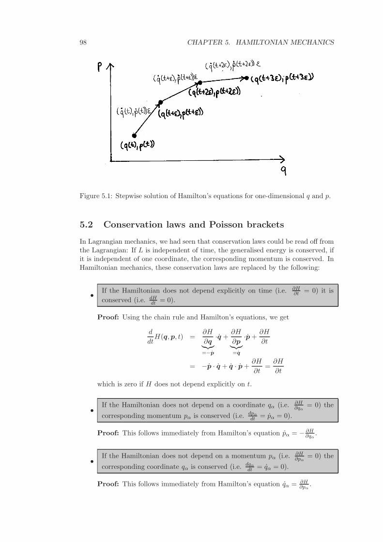
98 CHAPTER 5. HAMILTONIAN MECHANICS
Figure 5.1: Stepwise solution of Hamilton’s equations for one-dimensional q and p.
5.2 Conservation laws and Poisson brackets
In Lagrangian mechanics, we had seen that conservation laws could be read off fromthe Lagrangian: If L is independent of time, the generalised energy is conserved, ifit is independent of one coordinate, the corresponding momentum is conserved. InHamiltonian mechanics, these conservation laws are replaced by the following:
• If the Hamiltonian does not depend explicitly on time (i.e. ∂H∂t = 0) it is
conserved (i.e. dHdt = 0).
Proof: Using the chain rule and Hamilton’s equations, we get
d
dtH(q,p, t) =
∂H
∂q︸︷︷︸
=−p
·q +∂H
∂p︸︷︷︸
=q
·p +∂H
∂t
= −p · q + q · p +∂H
∂t=
∂H
∂t
which is zero if H does not depend explicitly on t.
• If the Hamiltonian does not depend on a coordinate qα (i.e. ∂H∂qα
= 0) the
corresponding momentum pα is conserved (i.e. dpα
dt = pα = 0).
Proof: This follows immediately from Hamilton’s equation pα = − ∂H∂qα
.
• If the Hamiltonian does not depend on a momentum pα (i.e. ∂H∂pα
= 0) the
corresponding coordinate qα is conserved (i.e. dqα
dt = qα = 0).
Proof: This follows immediately from Hamilton’s equation qα = ∂H∂pα
.
5.2. CONSERVATION LAWS AND POISSON BRACKETS 99
Compared to Lagrangian mechanics we see that the first conservation law has acleaner form (only H shows up, not L and h) and that there is a new conservationlaw for coordinates; the latter appears because coordinates and momenta are treatedon equal footing.
How do arbitrary functions F (q,p, t) change in time?
A conserved quantity need not be a coordinate or a momentum. Hence we shouldalso find out when an arbitrary function F (q,p, t) is conserved and how it changesin time if it is not conserved. To do so we compute the total time derivative
dF
dt=
∂F
∂q· q +
∂F
∂p· p +
∂F
∂t.
If we now use Hamilton’s equations we obtain
dF
dt=
∂F
∂q· ∂H
∂p− ∂F
∂p· ∂H
∂p+
∂F
∂t. (5.11)
Here ∂F∂q
· ∂H∂p
− ∂F∂p
· ∂H∂p
is called the Poisson bracket of F and H. The generaldefinition of the Poisson bracket is:
Def.: The Poisson bracket of two functions F (q,p, t) and G(q,p, t) is given by
F,G =∂F
∂q· ∂G
∂p− ∂F
∂p· ∂G
∂q=
d∑
γ=1
(∂F
∂qγ
∂G
∂pγ− ∂F
∂pγ
∂G
∂qγ
)
.
With the Poisson bracket we can now restate Eq. (5.11) as follows:
The time derivative of a arbitrary function F (q,p, t) is given by
dF
dt= F,H +
∂F
∂t.
This leads to the following conservation law:
If F is independent of t, i.e. F = F (q,p), then it is a conserved quantity if itsPoisson bracket with the Hamiltonian vanishes, i.e. if F,H = 0.
Poisson brackets allow to check easily whether a given quantity is conserved.
Examples
a) Fundamental Poisson brackets
The simplest Poisson brackets are those between coordinates and momenta. Theyhave the following form:
qα, qβ = 0
pα, pβ = 0
qα, pβ = δαβ .
We see that all Poisson brackets between coordinates and momenta vanish exceptthe one involving a coordinate and the corresponding momentum.
100 CHAPTER 5. HAMILTONIAN MECHANICS
Proof: The first two formulas are trivial: When the functions F and G areboth coordinates, the derivatives ∂F
∂pand ∂G
∂pin the definition of F,G vanish and
the result is zero. Similarly when the functions F and G are both momenta, thederivatives ∂F
∂qand ∂G
∂qvanish and again the Poisson bracket is zero. The Poisson
bracket involving coordinates and momenta
qα, pβ =
d∑
γ=1
(∂qα
∂qγ
∂pβ
∂pγ− ∂qα
∂pγ
∂pβ
∂qγ
)
.
is more complicated. To evaluate it we note that the derivative ∂qα
∂qγis 1 if α = γ and
0 otherwise. Hence it can be written as the Kronecker delta δαβ . For the momenta
we similarly have∂pβ
∂pγ= δβγ . In contrast the derivatives ∂qα
∂pγand
∂pβ
∂qγare always
zero. We thus obtain
qα, pβ =d∑
γ=1
δαγδβγ .
Here the summand is 1 if all coefficients coincide, i.e., if α = β = γ. Otherwise it iszero. Hence for α 6= β all summands are zero, while for α = β one summand is 1.The sum thus yields
qα, pβ = δαβ
as required.
b) Components of the angular momentum
We now evaluate the Poisson brackets involving the components of the angularmomentum
l = r × p =
xyz
×
px
py
pz
,
i.e.,
lx = ypz − zpy
ly = zpx − xpz
lz = xpy − ypx .
The Poisson bracket of the first two components is
lx, ly =∂lx∂x
∂ly∂px
+∂lx∂y
∂ly∂py
+∂lx∂z
∂ly∂pz
− (lx ↔ ly)
where (lx ↔ ly) indicates the last three summands of the Poisson bracket for which
the roles of lx and ly are interchanged. Now we can use that ∂lx∂x = 0,
∂ly∂y = 0,
∂lx∂px
= 0 and∂ly∂py
= 0. This leaves only two summands, and we get
lx, ly =∂lx∂z
∂ly∂pz
− ∂ly∂z
∂lx∂pz
= (−py)(−x) − pxy = lz .
We thus see that the Poisson bracket of the first two components of the angularmomentum yields the third component.
5.2. CONSERVATION LAWS AND POISSON BRACKETS 101
Properties of Poisson brackets
We will now derive a few rules that simplify the computation of more complicatedPoisson brackets. Here F,F1, F2, G,H are functions of q, p (and possibly time),and a1 and a2 are numbers.
1. Linearity:a1F1 + a2F2, G = a1F1, G + a2F2, G
2. Antisymmetry:F,G = −G,F
3. Product rule:FG,H = FG,H + GF,H
4. Jacobi identity:
F,G,H + G,H, F + H,F, G = 0
These rules imply that we should think of F,G as a kind of cross product ofphase-space functions. It should be a product since the definition involves productsof derivatives of F and G; also the linearity property is expected to hold for prod-ucts. However like the cross product, this product is an antisymmetric one, since itchanges sign if the two factors are interchanged.
Let us now prove these rules:
1. Linearity can be checked trivially if we insert a1F1 + a2F2 into the definitionof the Poisson bracket.
2. To prove antisymmetry we rearrange the terms in F,G and see that theresult coincides with −G,F:
F,G =∂F
∂q· ∂G
∂p− ∂F
∂p· ∂G
∂q
= −(
∂G
∂q· ∂F
∂p− ∂G
∂p· ∂F
∂q
)
= −G,F .
3. To prove the product rule for the Poisson bracket, we use the product rule forderivatives:
FG,H =∂(FG)
∂q· ∂H
∂p− ∂(FG)
∂p· ∂H
∂q
= F∂G
∂q· ∂H
∂p+ G
∂F
∂q· ∂H
∂p− F
∂G
∂p· ∂H
∂q− G
∂F
∂p· ∂H
∂q
= FG,H + GF,H
4. The proof of Jacobi’s identity is a bit messy. It is listed below for complete-ness:
For simplicity we’ll consider the case of one degree of freedom. The calculation inhigher dimensions is essentially the same; the only complication is keeping track ofindices.
102 CHAPTER 5. HAMILTONIAN MECHANICS
Let F = F (q, p), G = G(q, p) and H = H(q, p) be functions on phase space. We wishto show that
F, G, H + G, H, F + H, F, G = 0. (5.12)
Let’s evaluate the first term explicitly. We have that
F, G = FqGp − FpGq,
where Fq = ∂F/∂q, and similarly Fp, Gq and Gp. Then
F, G, H =∂F, G
∂qHp − ∂F, G
∂pHq
=∂(FqGp − FpGq)
∂qHp − ∂(FqGp − FpGq)
∂pHq,
or
F, G, H = (FqqGp+FqGpq−FpqGq−FpGqq)Hp−(FqpGp+FqGpp−FppGq−FpGqp)Hq,(5.13)
where Fqq = ∂2F/∂q∂q, and similarly for Fqp, Fpp, Gqq, etc. Note that Fqp = Fpq, i.e.,the ordering of mixed partials doesn’t matter; similarly for Gqp and Hqp. Similarly,for the other two terms in (5.12),
G, H, F = (GqqHp+GqHpq−GpqHq−GpHqq)Fp−(GqpHp+GqHpp−GppHq−GpHqp)Fq,(5.14)
and
H, F, G = (HqqFp+HqFpq−HpqFq−HpFqq)Gp−(HqpFp+HqFpp−HppFq−HpFqp)Gq .(5.15)
Now it is simply a matter of adding together terms from (5.13), (5.14) and (5.15) to
see that everything cancels. For example, consider the term FqqGpHp. This appears
in both (5.13) and (5.15), but with opposite signs. Likewise, you can check that every
other term appears in just two of the expressions (5.13), (5.14) and (5.15) but with
opposite signs.
In the rules 1, 3 and 4 above always the first argument of the Poisson bracket wassomething interesting (a sum, a product or another Poisson bracket). Completelyanalogous rules hold if the second argument is a sum, product or Poissonbracket. They can all be proven from the rules already derived, if we use theantisymmetry rule to interchange the two arguments.
Example
To illustrate the above rules let us evaluate the Poisson bracket py, lz:py, lz = py, xpy − ypx
= py, xpy − py, ypx= py, xpy + py, pyx − py, ypx − py, pyy= −py, ypx
= y, pypx
= px
Here we used linearity to get from the first to the second line, and the productrule to get from the second to the third line. The third line then contains onlyPoisson brackets of coordinates and momenta, which vanish apart from the term−py, y. Finally we used antisymmetry and the fundamental Poisson brackets toget −py, y = y, py = 1.
5.3. CANONICAL TRANSFORMATIONS 103
Example (optional)
Consider a phase space with one coordinate q and one momentum p. Let us evaluate the Poisson bracket of qα cos(βp) andqα sin(βp):
qα
cos β(βp), qα
sin(βp) = qαcos(βp), q
αsin(βp) + cos(βp)q
α, q
αsin(βp)
= qα
qαcos(βp), sin(βp) + q
αsin(βp)cos(βp), q
α + cos(βp)q
αq
α, sin(βp) + cos(βp) sin(βp)q
α, q
α
= 0 + qα
sin(βp)
−
∂ cos(βp)
∂p
∂qα
∂q
!+ cos(βp)q
α
∂qα
∂q
∂ sin(βp)
∂p
!+ 0
= αβ sin2(βp)q
2α−1+ αβ cos
2(βp)q
2α−1
= αβq2α−1
In the first two lines we used the product rule. Then the derivatives were evaluated.
Applications
As mentioned above, Poisson brackets can be used to check whether a quantityis conserved. Moreover Poisson brackets can be used to generate new conser-vation laws. This is due to Poisson’s theorem:
Poisson’s theorem: If two phase-space functions A(q,p) and B(q,p) are con-served then their Poisson bracket A,B is conserved as well.
Proof: We assume that A and B are conserved, i.e., that their Poisson bracketwith the Hamiltonian H vanishes. We then use the Jacobi identity to evaluate thePoisson bracket of A,B with H. The result is zero:
A,B,H = −B,H︸ ︷︷ ︸
=0
, A − H,A︸ ︷︷ ︸
=0
, B = 0 .
Hence the Poisson bracket of A,B with H vanishes and A,B is a conservedquantity.
We can thus get additional conserved quantities of a system by computing thePoisson brackets of the conserved quantities we already know. For example, if weknow that lx and ly are conserved then their Poisson bracket lx, ly = lz must beconserved as well, and if py and lz are conserved the same must hold for py, lz =px. However computing Poisson brackets need not always give something new; thePoisson bracket A,B may also be linearly dependent of A and B or trivial (say,zero).
5.3 Canonical transformations
A strong advantage of Lagrangian mechanics was that it the equations of motionhave the same form in all systems of coordinate. This freedom of picking coordinatesbecomes even larger in Hamiltonian mechanics: Now we can perform coordinatetransformations in phase space, including transformations that mix generalisedcoordinates and generalised momenta. Not all of these transformations willbe useful, but only those in which the basic ingredients of Hamiltonian mechanics(such as the Poisson brackets) remain the same. These transformation are calledcanonical transformations and defined as follows:
104 CHAPTER 5. HAMILTONIAN MECHANICS
Def.: Consider a transformation of coordinates in phase space
Qα = Qα(q,p)
Pα = Pα(q,p)
and the Poisson bracket defined by derivatives w.r.t. Q and P
F,GQ,P ≡ ∂F
∂Q· ∂G
∂P− ∂F
∂P· ∂G
∂Q.
The transformation is called canonical if the Poisson bracket F,GQ,P coincideswith F,G = ∂F
∂q· ∂G
∂p− ∂F
∂p· ∂G
∂qif we insert for F and G the coordinates and
momenta,
qα, qβQ,P = qα, qβ = 0
pα, pβQ,P = pα, pβ = 0
qα, pβQ,P = qα, pβ = δαβ . (5.16)
In other words, canonical transformations preserve the fundamental Poisson brack-ets.
Example: Consider a system with just one coordinate q and one momenum p.We can now define a transformation that just interchanges the coordinate and themomentum and flips a sign:
Q = −p
P = q
This transformation is canonical because
q, qQ,P = 0
p, pQ,P = 0
q, pQ,P =∂q
∂Q
∂p
∂P− ∂q
∂P
∂p
∂Q=
∂P
∂Q
∂(−Q)
∂P− ∂P
∂P
∂(−Q)
∂Q= 1 .
Here the first two lines are trivial as the Poisson bracket of any quantity with itselfis zero.
Thm.: If the transformation leading from q,p to Q,P is canonical we haveF,GQ,P = F,G for all phase-space functions F and G. In other words,canonical transformations preserve all Poisson brackets.
Proof: We assume that (5.16) holds and try to show that F,GQ,P = F,G.
5.3. CANONICAL TRANSFORMATIONS 105
We get
F,GQ,P =∂F
∂Q· ∂G
∂P− ∂F
∂P· ∂G
∂Q
=
d∑
α=1
(∂F
∂qα
∂qα
∂Q+
∂F
∂pα
∂pα
∂Q
)
·d∑
β=1
(∂G
∂qβ
∂qβ
∂P+
∂G
∂pβ
∂pβ
∂P
)
−[
∂
∂Q↔ ∂
∂P
]
=
d∑
α=1
d∑
β=1
∂F
∂qα
∂G
∂qβ
(∂qα
∂Q· ∂qβ
∂P− ∂qα
∂P· ∂qβ
∂Q
)
︸ ︷︷ ︸
=qα,qβQ,P =0
+∂F
∂qα
∂G
∂pβ
(∂qα
∂Q· ∂pβ
∂P− ∂qα
∂P· ∂pβ
∂Q
)
︸ ︷︷ ︸
=qα,pβQ,P =δαβ
+∂F
∂pα
∂G
∂qβ
(∂pα
∂Q· ∂qβ
∂P− ∂pα
∂P· ∂qβ
∂Q
)
︸ ︷︷ ︸
=pα,qβQ,P =−qβ ,pαQ,P =−δαβ
+∂F
∂pα
∂G
∂pβ
(∂pα
∂Q· ∂pβ
∂P− ∂pα
∂P· ∂pβ
∂Q
)
︸ ︷︷ ︸
=pα,pβQ,P =0
=d∑
α=1
(∂F
∂qα
∂G
∂pα− ∂F
∂pα
∂G
∂qα
)
= F,G .
In the first line, I simply wrote down the definition of the Poisson bracket. Inthe second line, the first two derivatives were evaluated using the chain rule (i.e.,∂F∂Q
=∑d
α=1
(∂F∂qα
∂qα
∂Q+ ∂F
∂pα
∂pα
∂Q
)
, and it was noted that ∂F∂P
· ∂G∂Q
can be obtained
from ∂F∂Q
· ∂G∂P
by interchanging the derivatives w.r.t. Q and P . Then the derivativeswere grouped together to obtain the fundamental Poisson brackets.
Hamilton’s equations
Canonical transformation also preserve Hamilton’s equations.
Thm.: If the transformation q,p → Q,P is time independent and canonical, wehave
Qα =∂H
∂Pα
Pα = − ∂H
∂Qα,
i.e., if we express the Hamiltonian in terms of Q, P and take derivatives w.r.t.these quantities we get Hamilton’s equations just as for q, p.

106 CHAPTER 5. HAMILTONIAN MECHANICS
Proof: We have
Qα = Qα,H +∂Qα
∂t︸ ︷︷ ︸
=0
= Qα,HQ,P
=
d∑
β=1
( ∂Qα
∂Qβ︸ ︷︷ ︸
=δαβ
∂H
∂Pβ− ∂Qα
∂Pβ︸ ︷︷ ︸
=0
∂H
∂Qβ
)
=∂H
∂Pα
Here I used that the total time derivative of every phase space function can bewritten as a Poisson bracket with the Hamiltonian plus a partial time derivative.In our case the partial time derivative vanishes because the Qα’s do not dependexplicitly on time. Then the Poisson bracket was written in terms of Q,P , and inthis form it could be evaluated easily. Similarly we obtain
Pα = Pα,H +∂Pα
∂t︸︷︷︸
=0
= Pα,HQ,P
=d∑
β=1
( ∂Pα
∂Qβ︸ ︷︷ ︸
=0
∂H
∂Pβ− ∂Pα
∂Pβ︸︷︷︸
=δαβ
∂H
∂Qβ
)
= − ∂H
∂Qα.
Example
To illustrate canonical transformations, let us consider the one-dimensional har-monic oscillator. If we set the mass equal to 1, the harmonic oscillator has theHamiltonian
H =1
2p2 +
1
2ω2q2 .
Since H does not depend explicitly on time, it is a conserved quantity. This meansthat in phase space the particles can only move on trajectories for which H =12p2 + 1
2ω2q2 = const, i.e., on ellipses (or circles if ω = 1), see Fig. 5.2. But we stillhave to determine how fast the particles go along these ellipses.
The usual way to solve this problem would be to use Hamilton’s equations withvariables q and p. One thus gets
q =∂H
∂p= p
p = −∂H
∂q= −ω2q .
This yields q = p = −ω2q and thus q = A sin(ωt + φ) where A and φ are constants.For p we obtain p = q = Aω cos(ωt + φ).
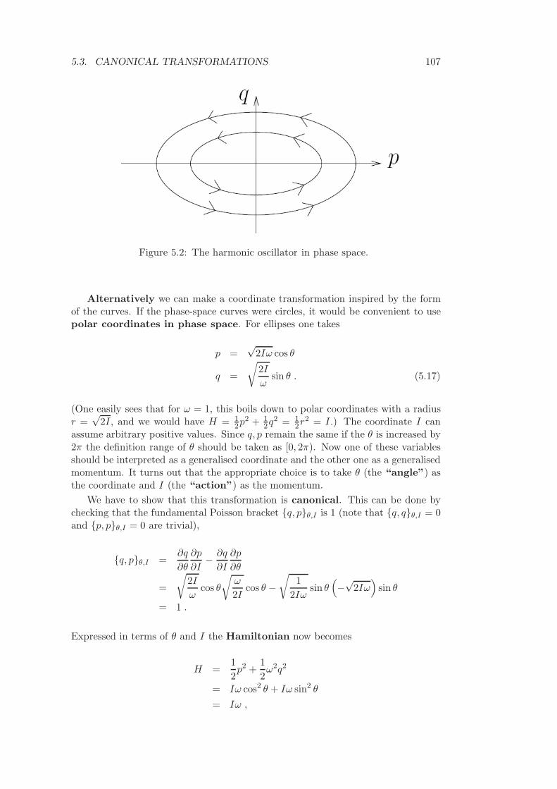
5.3. CANONICAL TRANSFORMATIONS 107
Figure 5.2: The harmonic oscillator in phase space.
Alternatively we can make a coordinate transformation inspired by the formof the curves. If the phase-space curves were circles, it would be convenient to usepolar coordinates in phase space. For ellipses one takes
p =√
2Iω cos θ
q =
√
2I
ωsin θ . (5.17)
(One easily sees that for ω = 1, this boils down to polar coordinates with a radiusr =
√2I, and we would have H = 1
2p2 + 12q2 = 1
2r2 = I.) The coordinate I canassume arbitrary positive values. Since q, p remain the same if the θ is increased by2π the definition range of θ should be taken as [0, 2π). Now one of these variablesshould be interpreted as a generalised coordinate and the other one as a generalisedmomentum. It turns out that the appropriate choice is to take θ (the “angle”) asthe coordinate and I (the “action”) as the momentum.
We have to show that this transformation is canonical. This can be done bychecking that the fundamental Poisson bracket q, pθ,I is 1 (note that q, qθ,I = 0and p, pθ,I = 0 are trivial),
q, pθ,I =∂q
∂θ
∂p
∂I− ∂q
∂I
∂p
∂θ
=
√
2I
ωcos θ
√ω
2Icos θ −
√
1
2Iωsin θ
(
−√
2Iω)
sin θ
= 1 .
Expressed in terms of θ and I the Hamiltonian now becomes
H =1
2p2 +
1
2ω2q2
= Iω cos2 θ + Iω sin2 θ
= Iω ,
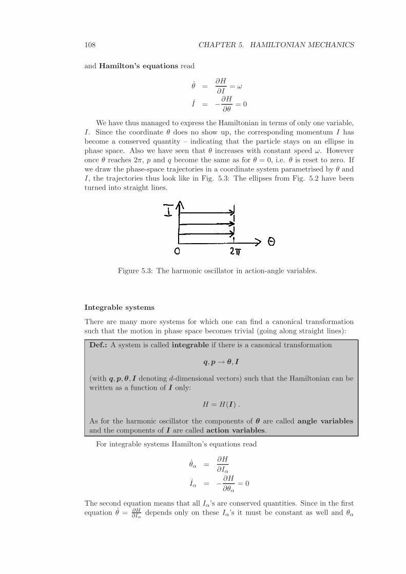
108 CHAPTER 5. HAMILTONIAN MECHANICS
and Hamilton’s equations read
θ =∂H
∂I= ω
I = −∂H
∂θ= 0
We have thus managed to express the Hamiltonian in terms of only one variable,I. Since the coordinate θ does no show up, the corresponding momentum I hasbecome a conserved quantity – indicating that the particle stays on an ellipse inphase space. Also we have seen that θ increases with constant speed ω. Howeveronce θ reaches 2π, p and q become the same as for θ = 0, i.e. θ is reset to zero. Ifwe draw the phase-space trajectories in a coordinate system parametrised by θ andI, the trajectories thus look like in Fig. 5.3: The ellipses from Fig. 5.2 have beenturned into straight lines.
Figure 5.3: The harmonic oscillator in action-angle variables.
Integrable systems
There are many more systems for which one can find a canonical transformationsuch that the motion in phase space becomes trivial (going along straight lines):
Def.: A system is called integrable if there is a canonical transformation
q,p → θ, I
(with q,p,θ, I denoting d-dimensional vectors) such that the Hamiltonian can bewritten as a function of I only:
H = H(I) .
As for the harmonic oscillator the components of θ are called angle variablesand the components of I are called action variables.
For integrable systems Hamilton’s equations read
θα =∂H
∂Iα
Iα = − ∂H
∂θα= 0
The second equation means that all Iα’s are conserved quantities. Since in the firstequation θ = ∂H
∂Iαdepends only on these Iα’s it must be constant as well and θα
5.3. CANONICAL TRANSFORMATIONS 109
increases linearly. Thus, expressed in terms of θ, I the phase-space motion indeedgoes along straight lines.
Now which systems are integrable? It is important that there must be d differ-ent conserved quantities Iα. For a one-dimensional system one conservation law (forthe energy) is enough, in higher-dimensional systems we need more. Also it mustbe possible to pick these quantities as momenta after a suitable canonical transfor-mation. Hence the must be mutually independent and their Poisson brackets Iα, Iβ
must vanish.Roughly speaking, integrable systems are “nice” systems which satisfy enough
conservation laws to allow for an analytical solution. Most systems considered inthis lecture are of this type. For example the spherical pendulum is decribed bytwo generalised coordinates and has two conserved quantities (the energy and theangular momentum), which we had already used to obtain an analytical solution.