CDS 301Fall, 2009

Image VisualizationChap. 9

November 5, 2009

Jie ZhangCopyright ©

Image Visualization

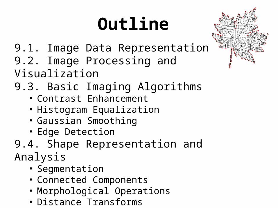
Outline9.1. Image Data Representation9.2. Image Processing and Visualization9.3. Basic Imaging Algorithms

• Contrast Enhancement• Histogram Equalization• Gaussian Smoothing• Edge Detection

9.4. Shape Representation and Analysis• Segmentation• Connected Components• Morphological Operations• Distance Transforms• Skeletonization

Image Data Representation

})({ iiii },{Φ}, {f}, {CpsD

• An image is a well-behaved uniform dataset.• An image is a two-dimensional array, or matrix

of pixels, e.g., bitmaps, pixmaps, RGB images• A pixel is square-shaped• A pixel has a constant value over the entire

pixel surface• The value is typically encoded in 8 bits integer

What is an image?

Image Processing and Visualization

• Image processing follows the visualization pipeline, e.g., image contrast enhancement following the rendering operation

• Image processing may also follow every step of the visualization pipeline

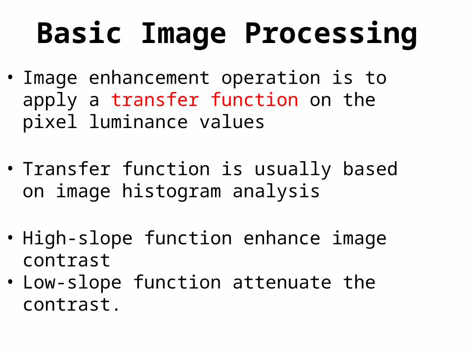
Basic Image Processing• Image enhancement operation is to apply a

transfer function on the pixel luminance values

• Transfer function is usually based on image histogram analysis

• High-slope function enhance image contrast• Low-slope function attenuate the contrast.

(Continued)

Image VisualizationChap. 9

November 12, 2009

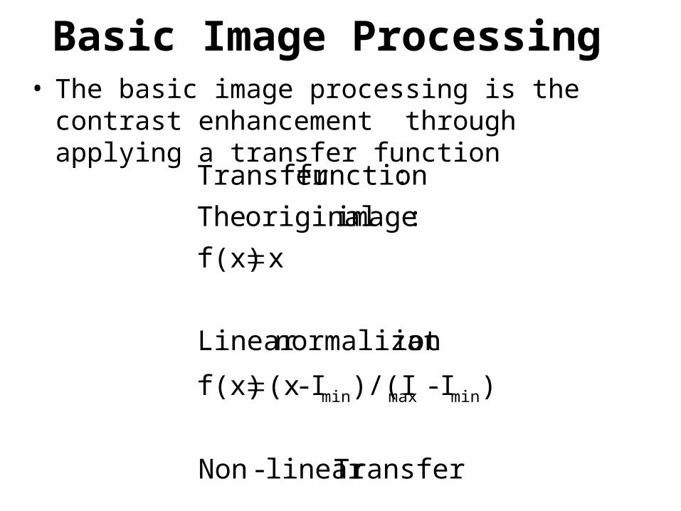
Basic Image Processing• The basic image processing is the contrast

enhancement through applying a transfer function

Transferlinear -Non

)I-)/(II-(xf(x)

ionnormalizatLinear

xf(x)

:image original The

:functionTransfer

minmaxmin

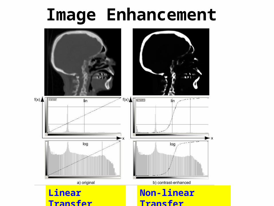
Image Enhancement

Linear Transfer Non-linear Transfer

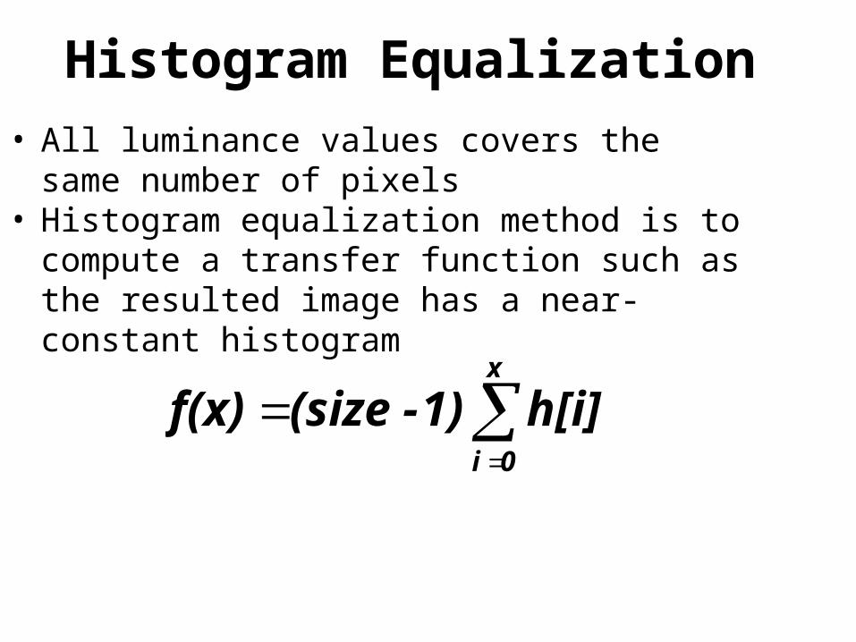
Histogram Equalization• All luminance values covers the same number

of pixels• Histogram equalization method is to compute a

transfer function such as the resulted image has a near-constant histogram

x

0i

h[i]1)-(sizef(x)

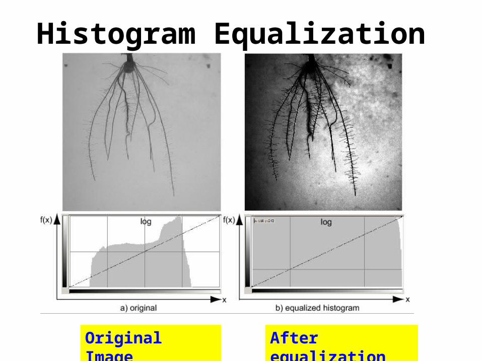
Histogram Equalization

Original Image After equalization

Smoothing

• Noise can be described as rapid variation of high amplitude

• Or regions where high-order derivatives of f have large values

• Noise is usually the high frequency components in the Fourier series expansion of the input signal

How to remove noise?

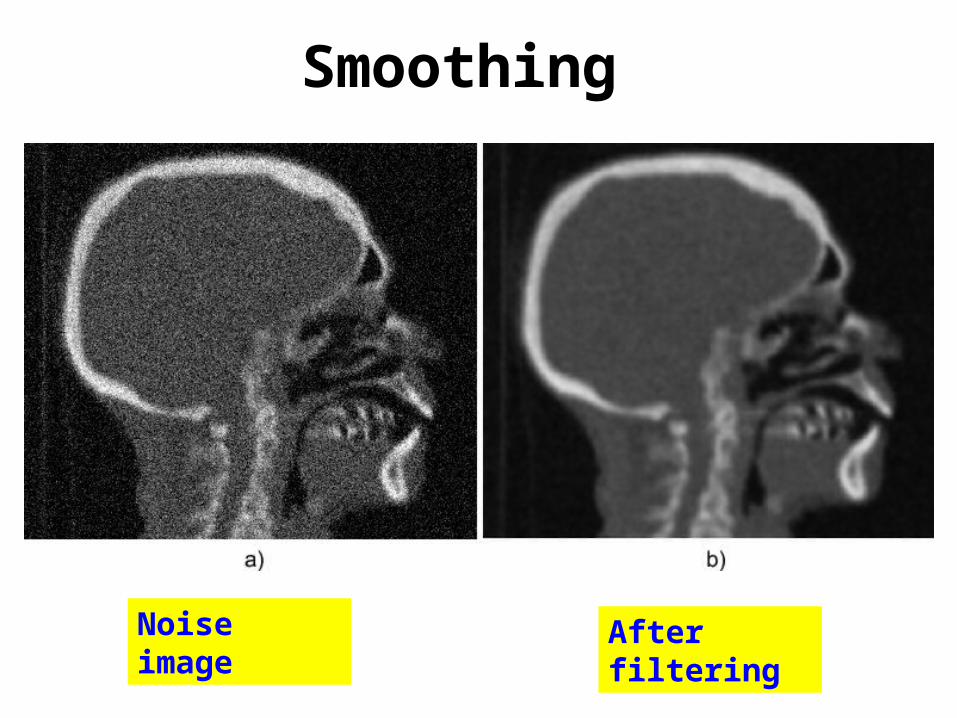
Smoothing

Noise image After filtering

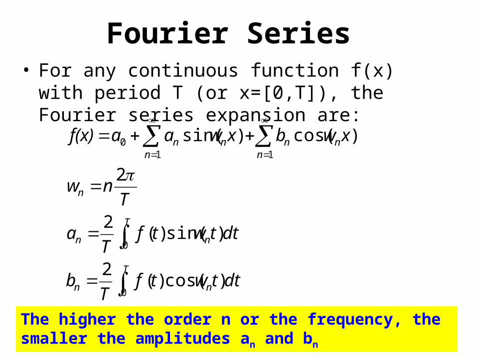
Fourier Series• For any continuous function f(x) with period T

(or x=[0,T]), the Fourier series expansion are:

T

nn

T

nn

n

nnn

nnn

dttwtfT

b

dttwtfT

a

Tnw

xwbxwaaf(x)

0

0

110

)cos()(2

)sin()(2

2

)cos()sin(

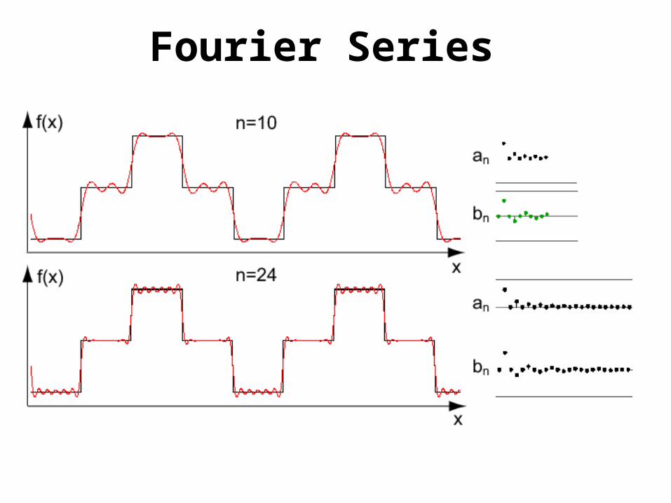
The higher the order n or the frequency, the smaller the amplitudes an and bn

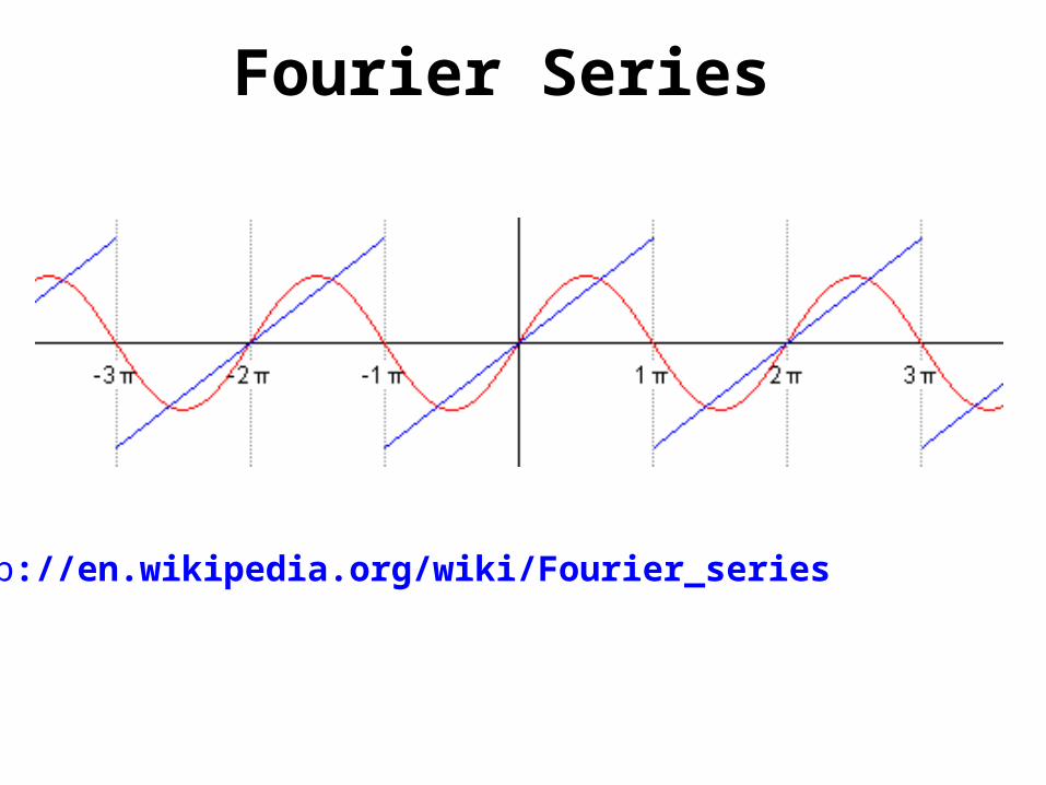
Fourier Series

http://en.wikipedia.org/wiki/Fourier_series

Fourier Series

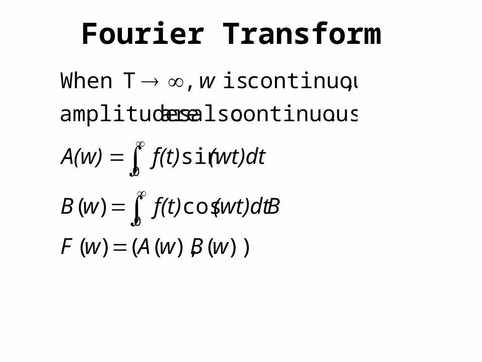
Fourier Transform

))(),(()(

cos)(

sin

.continuous also are amplitudes

,continuous is ,TWhen

0

0

wBwAwF

B(wt)dtf(t)wB

(wt)dtf(t)A(w)

w

Fourier Transform

Frequency Filtering

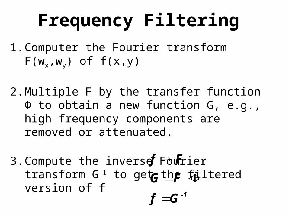
1. Computer the Fourier transform F(wx,wy) of f(x,y)

2. Multiple F by the transfer function Φ to obtain a new function G, e.g., high frequency components are removed or attenuated.

3. Compute the inverse Fourier transform G-1 to get the filtered version of f

1-Gf

FG

Ff

Frequency Filtering

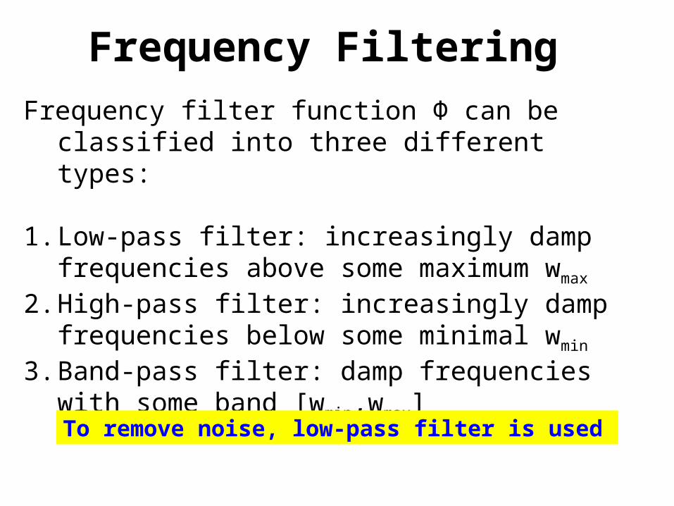
Frequency filter function Φ can be classified into three different types:

1. Low-pass filter: increasingly damp frequencies above some maximum wmax

2. High-pass filter: increasingly damp frequencies below some minimal wmin

3. Band-pass filter: damp frequencies with some band [wmin,wmax]

To remove noise, low-pass filter is used

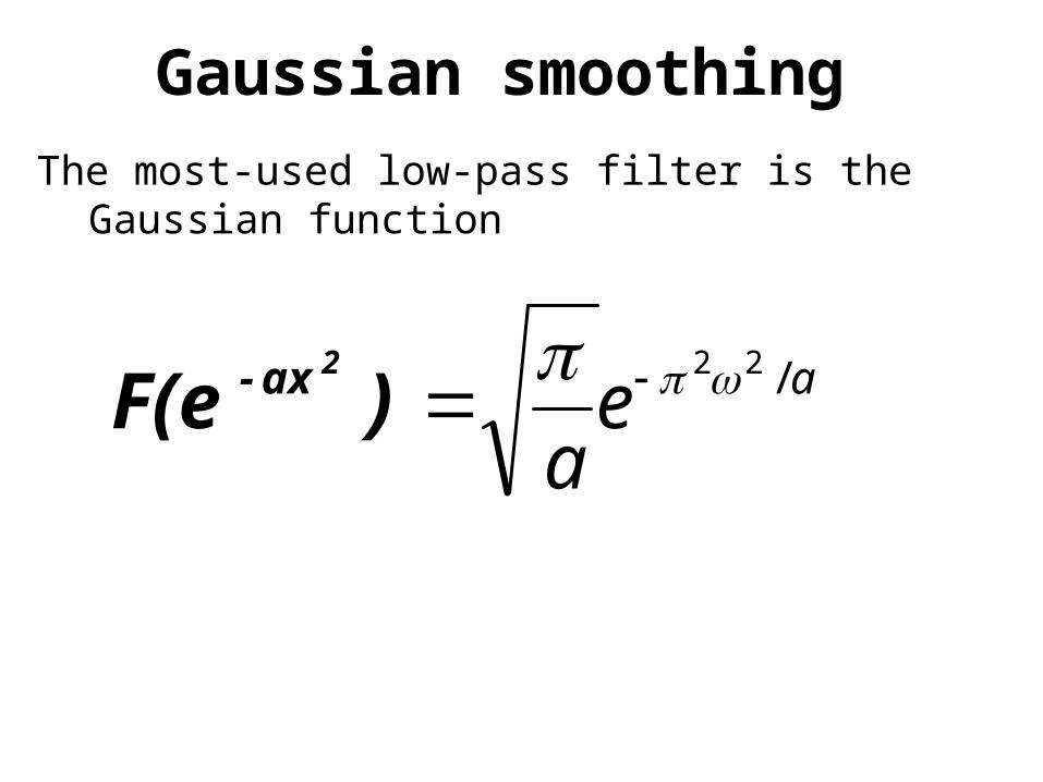
Gaussian smoothing

The most-used low-pass filter is the Gaussian function

aea

/22 )F(e2ax-

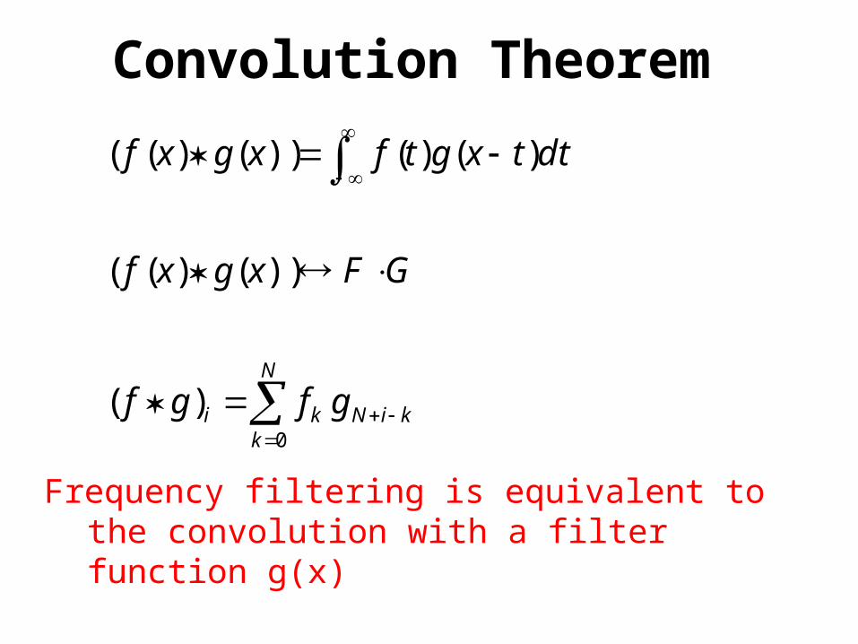
Convolution Theorem

Frequency filtering is equivalent to the convolution with a filter function g(x)

N

kkiNki gfgf

GFxgxf

dttxgtfxgxf

0

)(

))()((

)()())()((

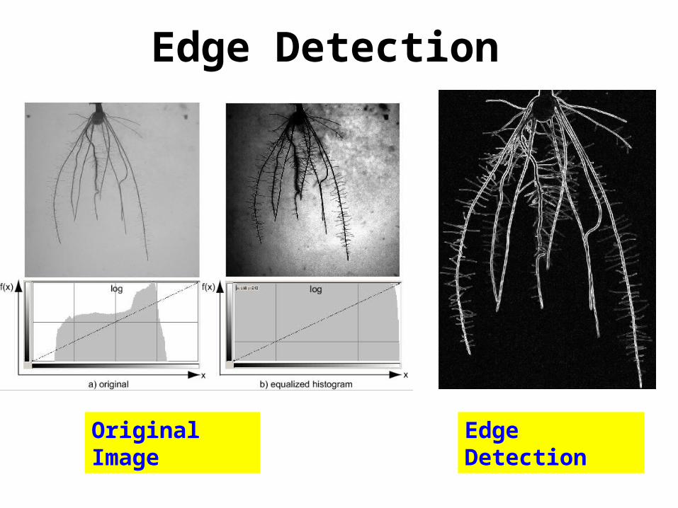
Edge Detection

Original Image Edge Detection

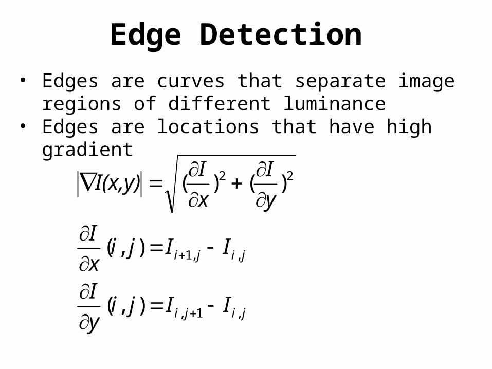
Edge Detection• Edges are curves that separate image regions of

different luminance• Edges are locations that have high gradient

jiji

jiji

IIjiy

I

IIjix

I

y

I

x

II(x,y)

,1,

,,1

22

),(

),(

)()(

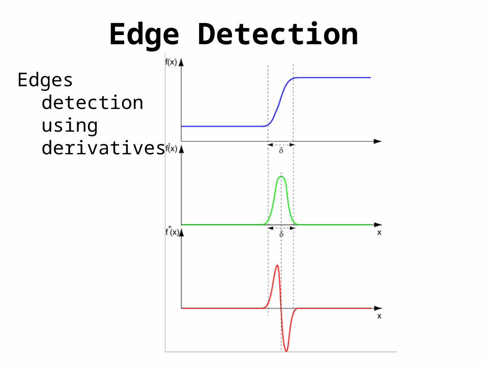
Edge Detection

Edges detection using derivatives

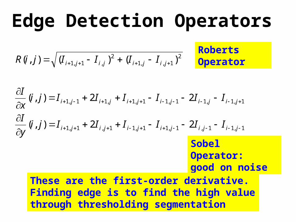
Edge Detection Operators

1,11,1,11,11,1,1

1,1,11,11,1,11,1

21,,1

2,1,1

22),(

22),(

)()(),(

jijijijijiji

jijijijijiji

jijijiji

IIIIIIjiy

I

IIIIIIjix

I

IIIIjiRRoberts Operator

Sobel Operator: good on noise

These are the first-order derivative. Finding edge is to find the high value through thresholding segmentation

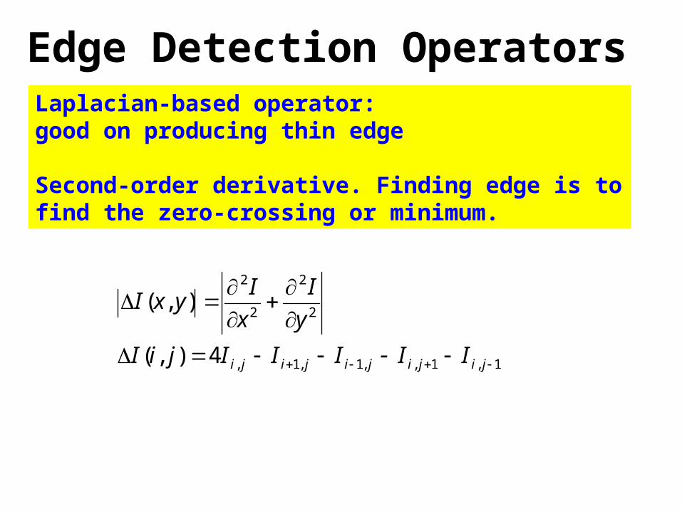
Edge Detection Operators

1,1,,1,1,

2

2

2

2

4),(

),(

jijijijiji IIIIIjiI

y

I

x

IyxI

Laplacian-based operator: good on producing thin edge

Second-order derivative. Finding edge is to find the zero-crossing or minimum.

(Continued)

Image VisualizationChap. 9

November 19, 2009

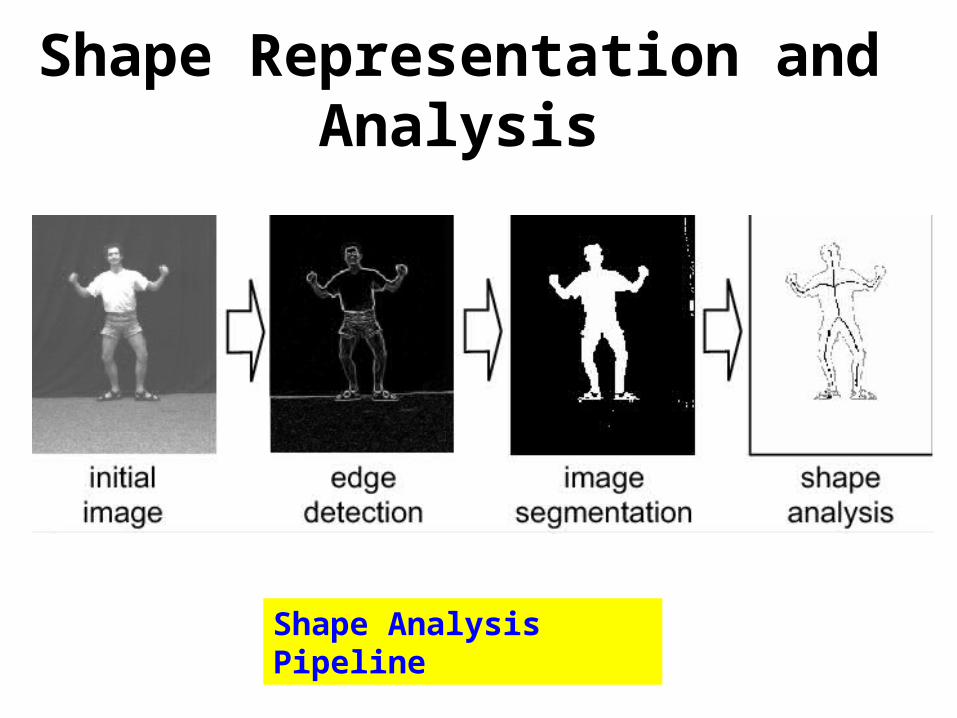
Shape Representation and Analysis

Shape Analysis Pipeline

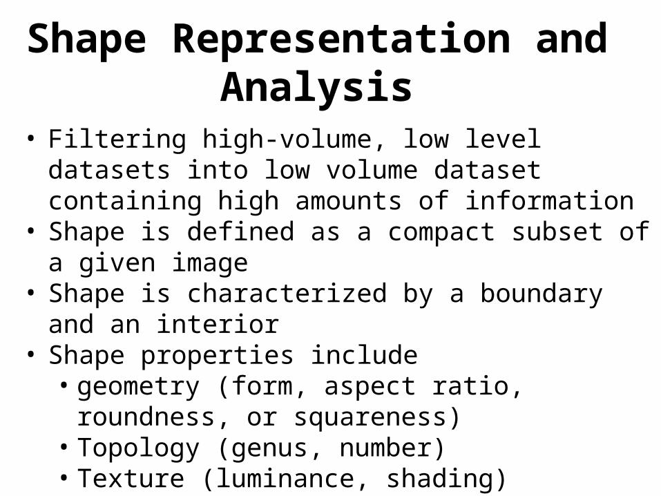
• Filtering high-volume, low level datasets into low volume dataset containing high amounts of information

• Shape is defined as a compact subset of a given image

• Shape is characterized by a boundary and an interior• Shape properties include

• geometry (form, aspect ratio, roundness, or squareness)

• Topology (genus, number)• Texture (luminance, shading)

Shape Representation and Analysis

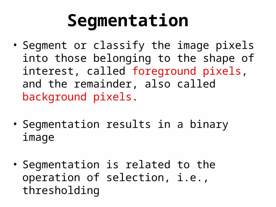
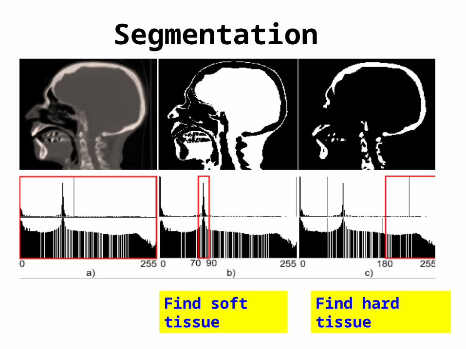
• Segment or classify the image pixels into those belonging to the shape of interest, called foreground pixels, and the remainder, also called background pixels.

• Segmentation results in a binary image

• Segmentation is related to the operation of selection, i.e., thresholding

Segmentation

Segmentation

Find soft tissue Find hard tissue

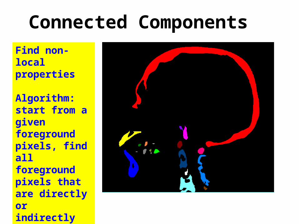
Connected ComponentsFind non-local properties

Algorithm: start from a given foreground pixels, find all foreground pixels that are directly or indirectly neighbored

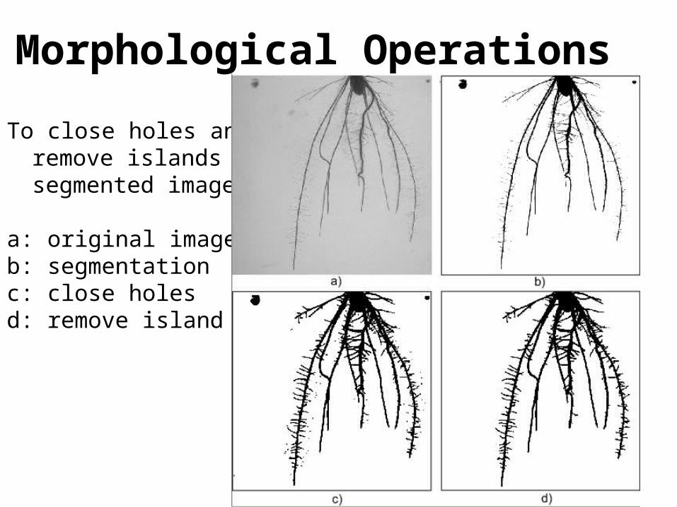
To close holes and remove islands in segmented images

a: original imageb: segmentationc: close holesd: remove island

Morphological Operations

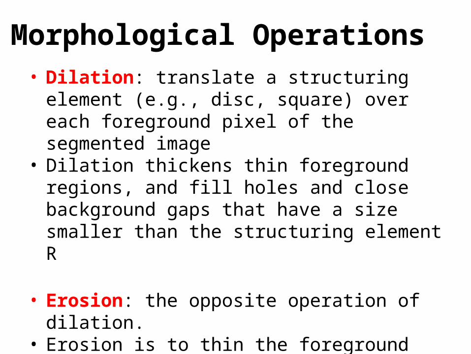
• Dilation: translate a structuring element (e.g., disc, square) over each foreground pixel of the segmented image

• Dilation thickens thin foreground regions, and fill holes and close background gaps that have a size smaller than the structuring element R

• Erosion: the opposite operation of dilation.• Erosion is to thin the foreground components,

remove island smaller than the structuring element R

Morphological Operations

• Morphological closing: dilation followed by an erosion

• Morphological opening: erosion followed by a dilation operation

Morphological Operations

Distance Transform

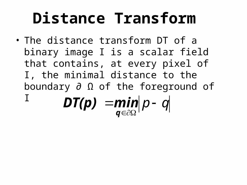
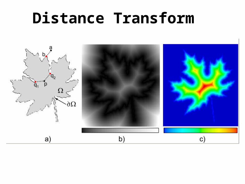
• The distance transform DT of a binary image I is a scalar field that contains, at every pixel of I, the minimal distance to the boundary ∂ Ω of the foreground of I

Distance Transform

qp q

minDT(p)

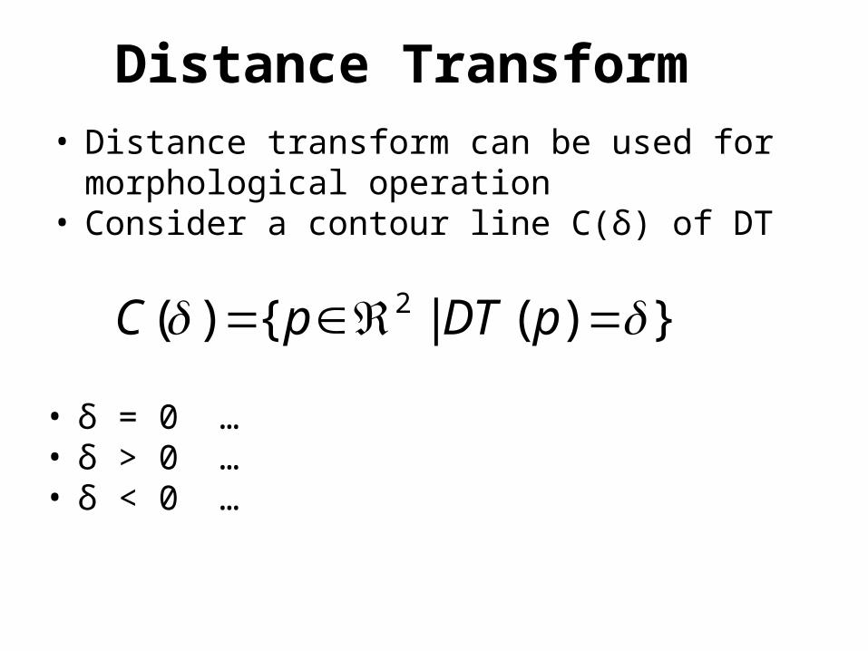
• Distance transform can be used for morphological operation

• Consider a contour line C(δ) of DT

Distance Transform

})(|{)( 2 pDTpC

• δ = 0 …• δ > 0 …• δ < 0 …

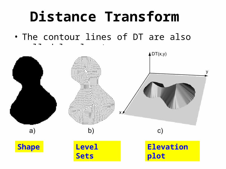
• The contour lines of DT are also called level sets

Distance Transform

Shape Level Sets Elevation plot

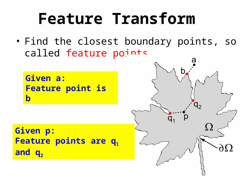
• Find the closest boundary points, so called feature points

Feature Transform

Given a:Feature point is b

Given p:Feature points are q1 and q2

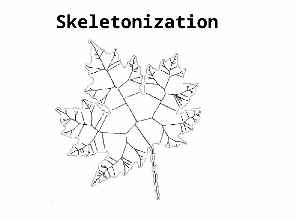
Skeletonization

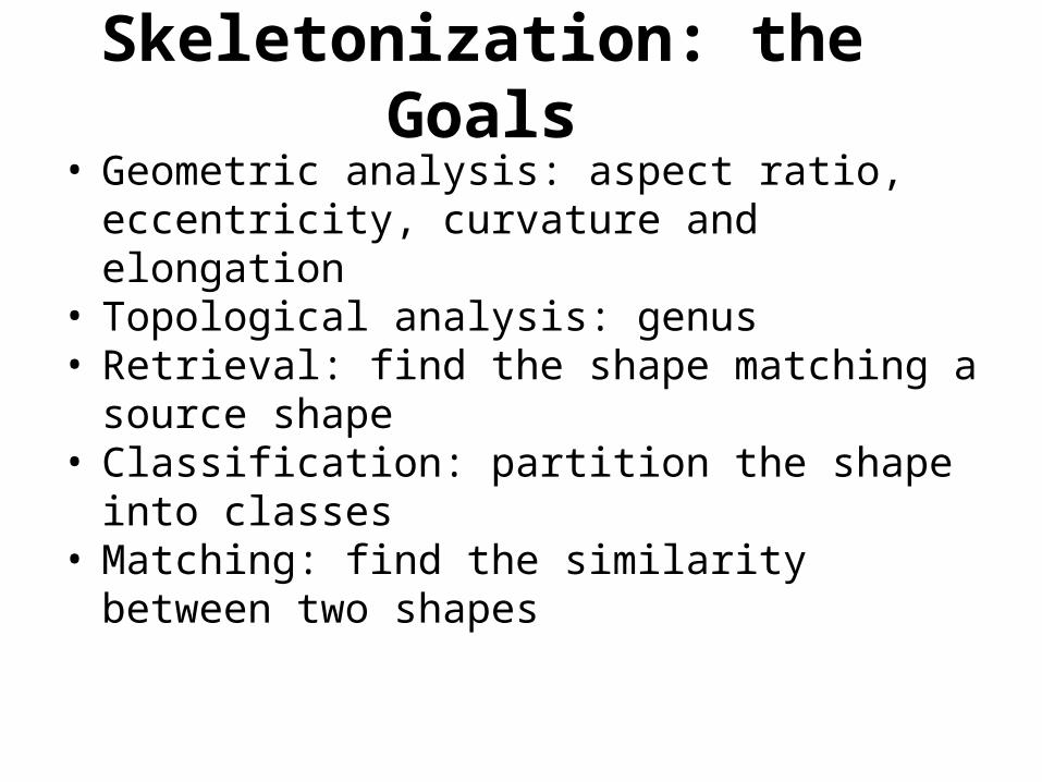
Skeletonization: the Goals• Geometric analysis: aspect ratio, eccentricity,

curvature and elongation• Topological analysis: genus• Retrieval: find the shape matching a source

shape• Classification: partition the shape into classes• Matching: find the similarity between two shapes

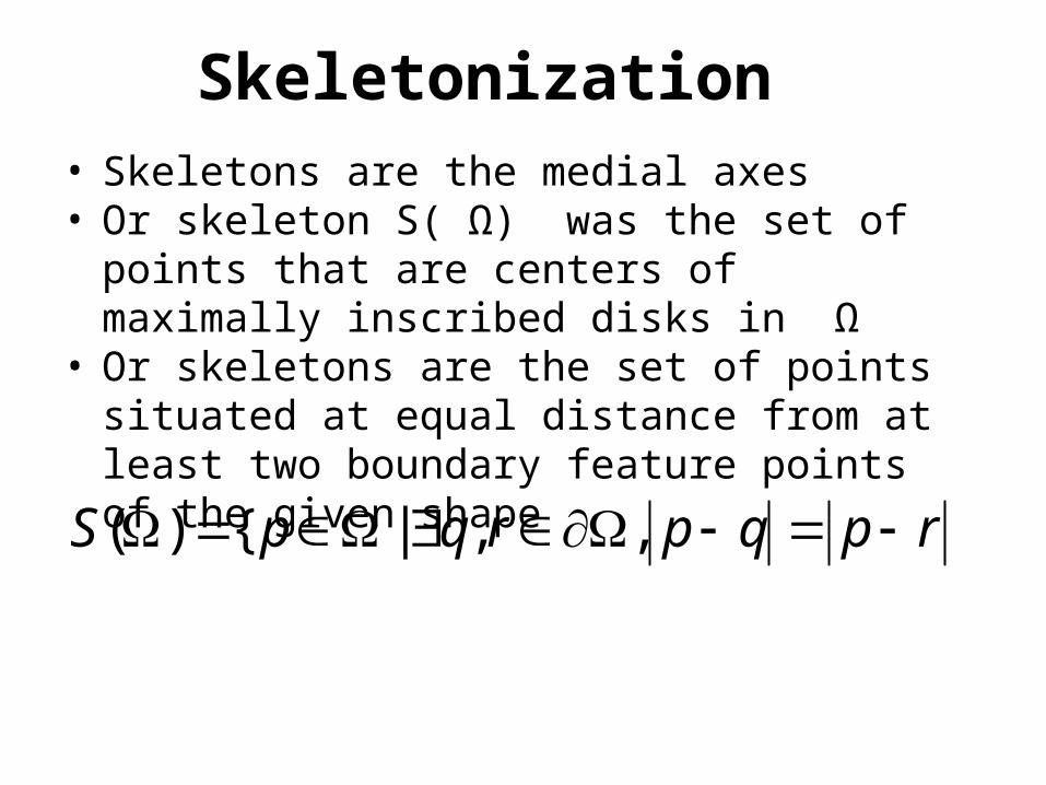
• Skeletons are the medial axes• Or skeleton S( Ω) was the set of points that

are centers of maximally inscribed disks in Ω• Or skeletons are the set of points situated at

equal distance from at least two boundary feature points of the given shape

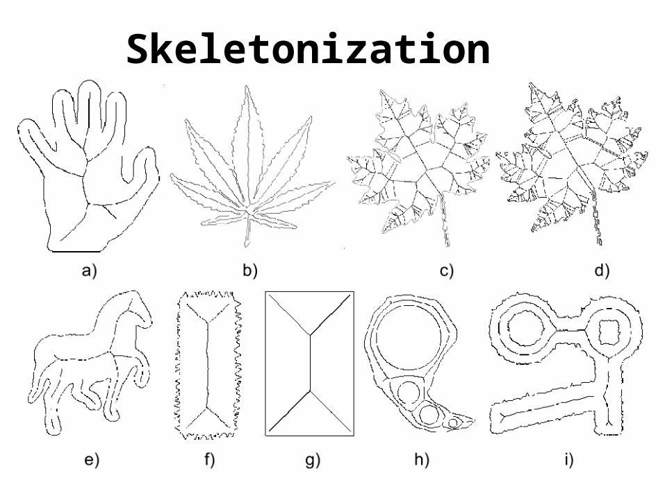
Skeletonization

rpqprqpS ,,|{)(

Skeletonization

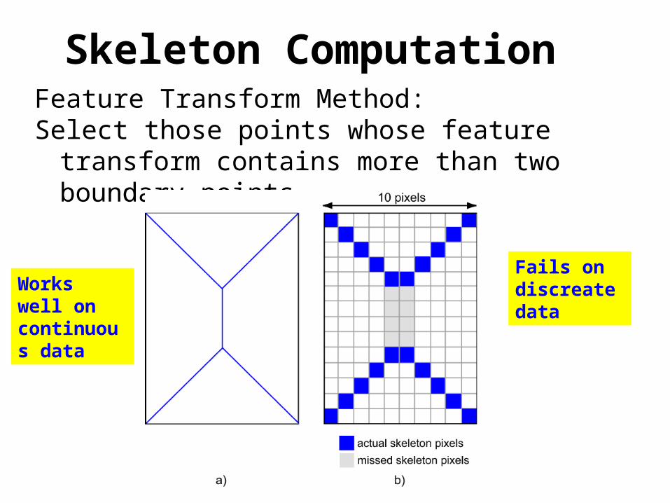
Feature Transform Method:Select those points whose feature transform

contains more than two boundary points.

Skeleton Computation

Works well on continuous data

Fails on discreate data

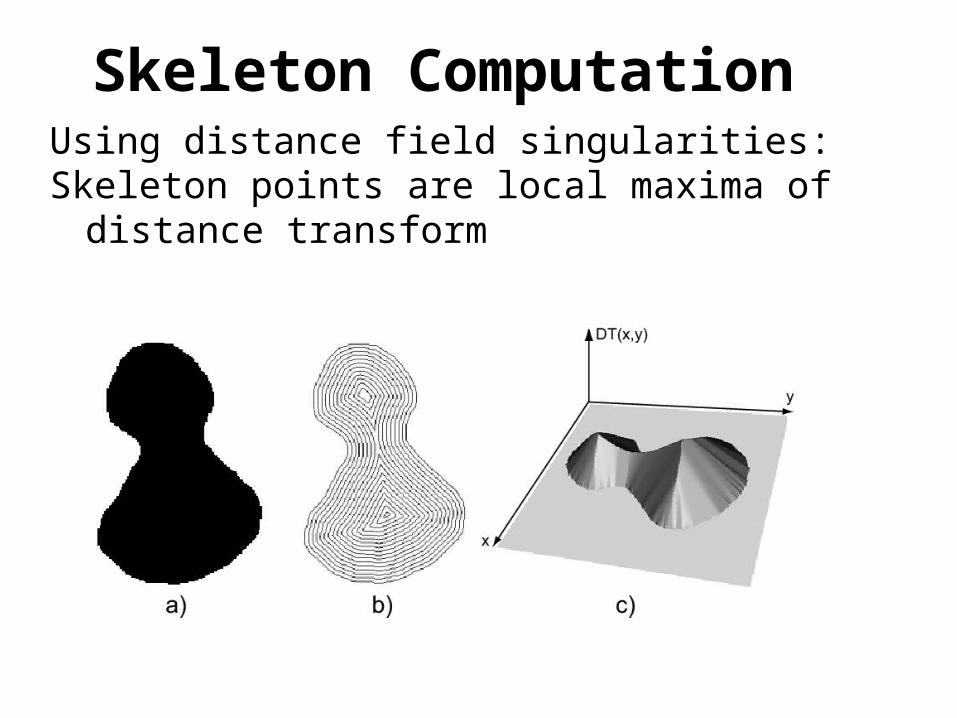
Using distance field singularities:Skeleton points are local maxima of distance

transform

Skeleton Computation

Endof Chap. 9

Note: covered all sections except 9.4.7 (skeleton in 3D)