CDS Auctions ∗

Mikhail Chernov,† Alexander S. Gorbenko,‡ and Igor Makarov§

October 13, 2011

Abstract We analyze credit default swap settlement auctions theoretically and eval-uate them empirically. In our theoretical analysis, we show that the current auctiondesign may not result in the fair bond price and suggest modifications to the auctiondesign to minimize mispricing. In our empirical study, we document that an auc-tion undervalues bonds by 10%, on average, on the day of the auction and link thisundervaluation to the number of bonds that are exchanged in the auction. We alsofind that underlying bond prices follow a V pattern around the auction day. In the10 days preceding the auction, prices decrease by 30% on average. In the 10 daysfollowing the auction, prices revert to their pre-auction levels.

JEL Classification Codes: G10, G13, D44

Keywords: credit default swaps, auctions, settlement, open interest

∗We thank Bruno Biais, Christopher Hennessy, Francis Longstaff, Oleg Rytchkov, DimitriVayanos and seminar participants at LBS, LSE, Nottingham University, and the Paul WoolleyCentre in Toulouse.†London School of Economics, and CEPR; m.chernov@lse.ac.uk.‡London Business School; agorbenko@london.edu.§London Business School; imakarov@london.edu.

Introduction

Credit Default Swaps (CDS) have been one of the most significant financial innova-

tions in the last 20 years. They have become very popular among both investment and

commercial banks, insurance companies, pension fund managers, and many other eco-

nomic agents. As a result, the market has experienced enormous growth. According

to the Bank of International Settlements (BIS), the notional amount of single-name

CDS contracts grew from $5.1 trillion in December 2004 to $33.4 trillion in June 2008,

and was still $18.4 trillion in June 2010 following a decline in the aftermath of the

credit crisis.

The recent crisis put CDS in the spotlight, with policymakers now assigning a

central role to CDS in many reforms. The success of these reforms depends on the

efficient functioning of the CDS market and on a thorough understanding of how it

operates. Recognizing this, a lot of research is dedicated to valuation of the contracts,

econometric analysis of CDS premia, studying violations of the law of one price in

the context of basis trades, impact of the search frictions, counterparty risk, private

information and moral hazard problems associated with holding both bonds and CDS

protection on the same entity.1

In this paper, we focus on another aspect of CDS. We study how the payoff

on a CDS contract is determined upon a credit event. Our theoretical analysis of

the unusual auction-based procedure reveals that this mechanism is vulnerable to

mispricing relative to the fundamental value. The mispricing is attributable, in large

part, to strategic bidding on the part of investors holding CDS. Empirically, we find

that CDS auctions underprice the underlying securities by 10%, on average. Because

this is an economically large magnitude, our findings may have implications for how

CDS are valued, used and analyzed.

In a nutshell, a CDS is a contract that protects a buyer against the loss of a bond’s

principal in the case of a credit event (e.g., default, liquidation, debt restructuring,

etc.). Initially, CDS were settled physically with the cheapest-to-deliver option. Un-

der such settlement, the protection buyer has to deliver any bond of the reference

1This work includes, but is not limited to, Acharya and Johnson (2007), Arora, Gandhi, andLongstaff (2009), Bolton and Oehmke (2011), Duffie (1999), Duffie and Zhu (2011), Garleanu andPedersen (2011), Longstaff, Mithal, and Neis (2005), Pan and Singleton (2008), and Parlour andWinton (2010).

entity to the protection seller in exchange for the bond’s par value. As a result of

the rapid development of the CDS market, the notional amount of outstanding CDS

contracts came to exceed the notional amount of deliverable bonds by many times.

This made physical settlement impractical and led the industry to develop a cash

settlement mechanism. This mechanism is the object of our study.

While a myriad of derivatives are settled in cash, the settlement of CDS in cash is

challenging for two reasons. First, the underlying bond market is opaque and illiquid,

which makes establishing the benchmark bond price for cash settlement difficult.

Second, parties with both the CDS and bond positions face recovery basis risk if

their positions are not closed simultaneously.2 The presence of this risk demands that

the settlement procedure include an option to replicate an outcome of the physical

settlement.

The industry has developed a novel two-stage auction in response to these chal-

lenges. At the first stage of the auction, parties that wish to replicate the outcome of

the physical settlement submit their requests for physical delivery via dealers. These

requests for physical delivery are aggregated into the net open interest (NOI). Deal-

ers also submit bid and offer prices with a commitment to transact in a predetermined

minimal amount at the quoted prices. These quotations are used to construct the

initial market midpoint price (IMM). The IMM is used to derive a limit on the

final auction price that is imposed to avoid a potential price manipulation. The

limit is referred to as the price cap. The NOI and the IMM are announced to all

participants.

At the second stage, a uniform divisible good auction is implemented, in which

the net open interest is cleared. Each participant can submit limit bids that are

combined with the bids of dealers from the first stage. The price of a bid that clears

the net open interest is declared to be the final auction price, which is then used to

settle the CDS contracts in cash.

We analyze the auction outcomes from both theoretical and empirical perspectives.

2Imagine a party that hedges a long position in a bond by buying a CDS with the same notionalamount. The final physically-settled position is known in advance: the protection buyer deliversa bond in exchange for the predetermined cash payment equal to the par value. However, thecash-settled position is uncertain before the auction: the protection buyer keeps the bond, paysthe uncertain auction-determined bond value to the protection seller, and receives par value inexchange. The difference between the market value of the bond held by the protection buyer andthe auction-determined value is the risky recovery basis.

2

To study price formation, we follow Wilson (1979) and Back and Zender (1993) and

formalize the auction using an idealized setup in which all auction participants are

risk-neutral and have identical expected valuations of the bond, v. This case is not

only tractable, but also provides a useful benchmark against which to test whether

the auction leads to the fair-value price. While Wilson (1979) shows that a standard

uniform divisible-good auction may result in underpricing, we demonstrate that the

current auction design can result in the final price being either above or below v.

The reason we arrive at the different conclusion is that participants can have

prior positions in the derivative contracts written on the asset being auctioned. If a

participant chooses to settle her entire CDS position physically then her final payoff

is not affected by the auction outcome. However, in the case of cash settlement,

buyers of protection benefit if the auction price is set below the fair value, while

sellers benefit if the price is set too high. Therefore, an auction outcome depends on

the size of the net CDS positions, that is, positions that remain after participants

submit their physical settlement requests.

To be specific, consider the case of positive NOI, that is, a second-stage auction

in which the agents buy bonds. When the net CDS positions of protection sellers are

less than the NOI then the Wilson (1979) logic still holds. An underpricing can occur

because auction participants may choose not to bid aggressively. The current auction

rule is such that their bids above the final price are guaranteed to be fully filled, so

they are not sufficiently rewarded for raising their bids. When the net CDS positions

of sellers are larger than the NOI, bidding above the fair value and realizing a loss

from buying NOI units of bonds is compensated by a reduction in the net pay on

the existing CDS contracts. Therefore, if there were no price cap, the auction price

would be no lower than v in this case.

Our theory delivers a rich set of testable predictions. Implementation of such

tests requires data on individual CDS positions and bids, which are not available.

Nonetheless, we are able to analyse some aspects of the auction data and find evidence

that is consistent with our theoretical predictions. We use TRACE bond data to

construct the reference bond price. Using the reference bond price from the day

before the auction as a proxy for v, we document that the auction price is set at

the price cap whenever there is overpricing. Furthermore, the extent of overpricing

does not exceed the spread between the price cap and IMM. When the final auction

3

price is not capped and the NOI is positive (which is a typical situation), the auction

undervalues bonds, and the degree of undervaluation increases with the NOI. In

addition, underlying bond prices follow a V pattern around the auction day. In the

10 days preceding the auction, prices decrease by 30%, on average. On the day of the

auction, bond prices reach their lowest value corresponding to auction underpricing

of 10%, on average. In the 10 days following the auction, prices revert to their pre-

auction levels. This evidence suggests that our conclusions are robust to our choice

of the reference bond price.

Our results documenting underpricing during the auction prompt us to consider

ways in which it might be possible to mitigate mispricing. In a standard setting, in

which agents have no prior positions in the derivative contracts written on the asset

being auctioned, Kremer and Nyborg (2004) suggest a likely source of underpricing

equilibria. They show that a simple change of the allocation rule from the pro-rata

on the margin to the pro-rata destroys all underpricing equilibria. We show that

the same change of the allocation rule would be beneficial in our setting as well. In

addition, we suggest that imposing an auction price cap conditional on the outcomes

of the first stage could further reduce mispricing in equilibrium outcomes.

To the best of our knowledge, there are three papers that examine CDS auctions.

Two of them simply analyse empirical data from CDS auctions. Helwege, Maurer,

Sarkar, and Wang (2009) evaluate an early sample of 10 auctions, of which only four

used the current auction format, and find no evidence of mispricing. Similarly to us,

Coudert and Gex (2010) document a large gap between a bond price on the auction

date and the final auction price by studying a somewhat different sample of auctions

and using Bloomberg data for reference bond prices. However, they do not link the

gap to the net open interest, nor do they provide any theoretical explanations for their

findings. Finally, in an independent and contemporaneous study, Du and Zhu (2011)

examine what types of outcome are possible in CDS auctions. Their paper considers a

special case of our model in which they implicitly assume that all market participants

can buy and short-sell bonds of distressed companies at the fair value v without any

restrictions. This setup implies that only overpricing equilibria can exist. Further,

they treat physical settlement requests as given. We show that this setup results in

fair pricing in an auction if agents choose physical settlement optimally. We allow

for a more realistic setup with short-sale constraints and in which some participants

4

cannot hold distressed debt. Similar to Wilson (1979) and Back and Zender (1993),

we show that there can be a substantial underpricing in this case.

The remainder of the paper is organized as follows. Section 1 describes the CDS

auction methodology that is currently used. Section 2 describes the auction model.

Section 3 provides the main theoretical analysis. Section 4 relates the predictions

of our theoretical model to empirical data from CDS auctions. Section 5 discusses

modifications that have the potential to improve the efficiency of the auction. Section

6 concludes. The appendix contains proofs that are are not provided in the main text.

1 The Auction Format

This discussion is based on a reading of the auction protocols, which are available

from the ISDA website. The Dura auction, conducted on November 28, 2006, was the

first auction that allowed single-name CDS to be settled in cash. All previous auctions

were designed for cash-settling credit indexes and used different rules. The auction

design used for Dura’s bankruptcy and all the subsequent credit events consists of

two stages.

In the first stage, participants in the auction submit their requests for physical

settlement. Each request for physical settlement is effectively an order to buy or

sell bonds at par and must be, to the best of the relevant party’s knowledge, in the

same direction as, and not in excess of, its market position. This element of the

design allows the participants to replicate the traditional physical settlement of the

contracts. For example, if a party is long by one unit of protection (directionally

equivalent to selling a bond) and submits a request to physically deliver one bond (as

if selling one bond at par), the resulting cash flow is identical to that of the physical

settlement.

In addition, a designated group of agents (dealers) makes a two-way market in

the defaulted assets by submitting bids and offers with a predefined maximum spread

and a predefined quotation size that is associated with it. The spread and quotation

sizes are subject to specification prior to each auction and may vary for each auction

depending on the liquidity of the defaulted assets.3

3The most common value of the spread is 2% of par. Quotation sizes range from $2 to $10 million;$2 million is the most common amount.

5

The inputs of the first stage are used to calculate a net open interest (NOI)

and an ‘initial market midpoint’ (IMM), which are carried into the second part

of the auction. The NOI is computed as a difference of the buy and sell requests

for physical settlement. The IMM is set by discarding crossing/touching bids and

offers, and taking the ‘best half’ of the bids and offers and calculating the average.

The best half would be, respectively, the highest bids, and the lowest offers. A dealer

makes a payment (an adjustment amount) to ISDA if her quotation is crossed and is

on the wrong side of the IMM , that is, if a bid is higher than the IMM, and the

NOI is to sell or if an offer is lower than the IMM , and the NOI is to buy. The

adjustment amount is a product of the quotation amount and the difference between

the quotation and IMM.

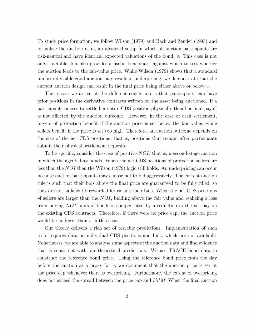
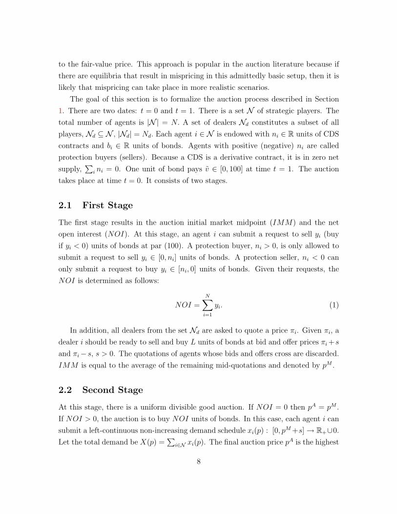
As an example, consider the Nortel Limited auction that took place on February

10, 2009. Table 1 lists the market quotes that were submitted. Next, all the bids

are sorted in the descending offer and all the offers are sorted in the ascending offer.

Then, the highest bid is matched with the lowest offer; the second highest bid is

matched with the second lowest offer; and so on. Figure 1 displays the quotes from

Table 1 that are organized this way. For example, we that the Citibank bid of 10.5

and the Barclays offer of 6.0 create a tradeable market.

IMM is computed based on the non-tradebale quotes. In our example, there are

nine pairs of such quotes. First, the “best half”, i.e. the first five pairs, of the non-

tradebale quotes is selected. Second, IMM is computed as an average of both bid

and offer quotes in the best half, rounded to the nearest one-eighth of one percentage

point. In our example, the relevant bids are: three times 7.0 and two times 6.5; the

relevant offers are: two times 8.0, two times 8.5, and 9. The average is 7.6 and the

rounded average is 7.625.

Given the established IMM and the direction of open interest, the dealers whose

quotes resulted in tradeable markets pay an adjustment amount to ISDA. In the

case of Nortel, the open interest was to sell. Thus, the dealers whose bids crossed

the markets has to pay an amount equal to (Bid-IMM) times the quotation amount,

which was $2 MM in the Nortel case. Thus, Citigroup had to pay (10.5−7.625)/100×$2MM = $57500 and Banc of America had to pay (9.5 − 7.625)/100 × $2MM =

$37500.

Finally, the direction of the open interest determines the cap on the final price

6

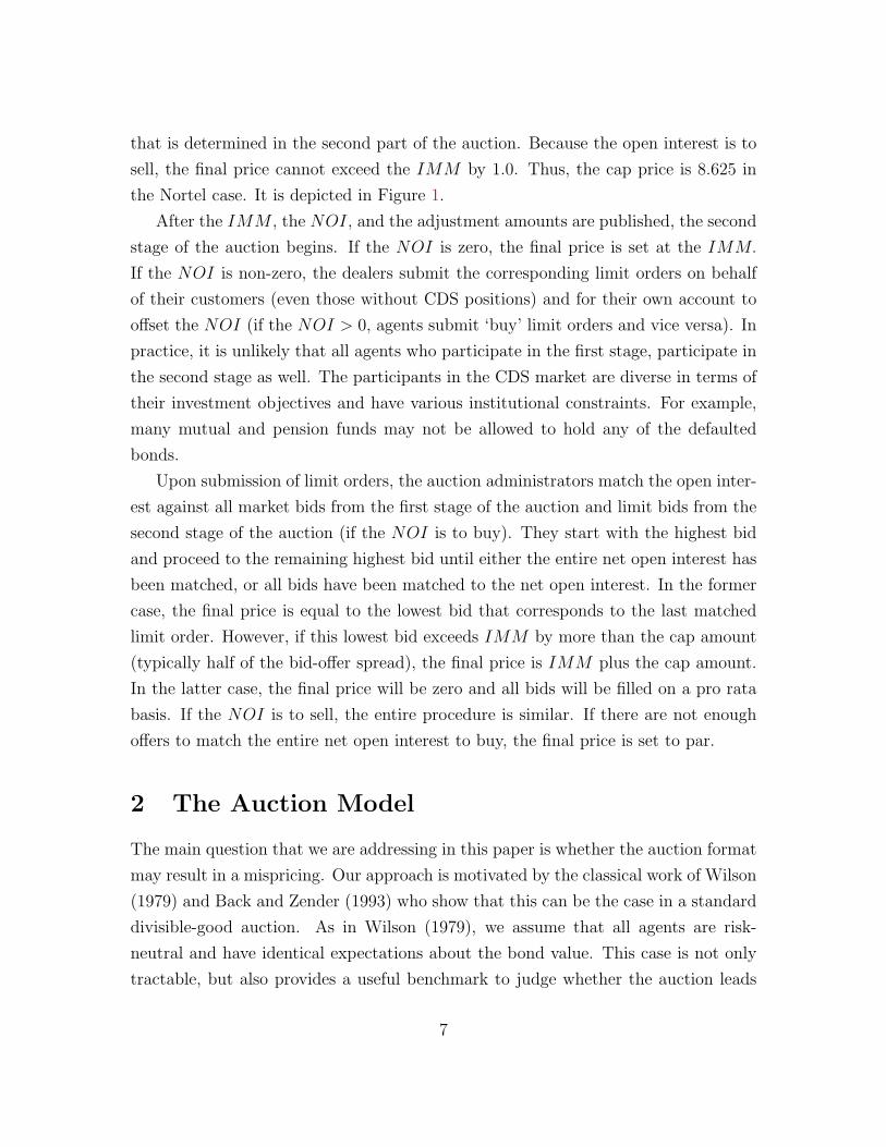
that is determined in the second part of the auction. Because the open interest is to

sell, the final price cannot exceed the IMM by 1.0. Thus, the cap price is 8.625 in

the Nortel case. It is depicted in Figure 1.

After the IMM , the NOI, and the adjustment amounts are published, the second

stage of the auction begins. If the NOI is zero, the final price is set at the IMM.

If the NOI is non-zero, the dealers submit the corresponding limit orders on behalf

of their customers (even those without CDS positions) and for their own account to

offset the NOI (if the NOI > 0, agents submit ‘buy’ limit orders and vice versa). In

practice, it is unlikely that all agents who participate in the first stage, participate in

the second stage as well. The participants in the CDS market are diverse in terms of

their investment objectives and have various institutional constraints. For example,

many mutual and pension funds may not be allowed to hold any of the defaulted

bonds.

Upon submission of limit orders, the auction administrators match the open inter-

est against all market bids from the first stage of the auction and limit bids from the

second stage of the auction (if the NOI is to buy). They start with the highest bid

and proceed to the remaining highest bid until either the entire net open interest has

been matched, or all bids have been matched to the net open interest. In the former

case, the final price is equal to the lowest bid that corresponds to the last matched

limit order. However, if this lowest bid exceeds IMM by more than the cap amount

(typically half of the bid-offer spread), the final price is IMM plus the cap amount.

In the latter case, the final price will be zero and all bids will be filled on a pro rata

basis. If the NOI is to sell, the entire procedure is similar. If there are not enough

offers to match the entire net open interest to buy, the final price is set to par.

2 The Auction Model

The main question that we are addressing in this paper is whether the auction format

may result in a mispricing. Our approach is motivated by the classical work of Wilson

(1979) and Back and Zender (1993) who show that this can be the case in a standard

divisible-good auction. As in Wilson (1979), we assume that all agents are risk-

neutral and have identical expectations about the bond value. This case is not only

tractable, but also provides a useful benchmark to judge whether the auction leads

7

to the fair-value price. This approach is popular in the auction literature because if

there are equilibria that result in mispricing in this admittedly basic setup, then it is

likely that mispricing can take place in more realistic scenarios.

The goal of this section is to formalize the auction process described in Section

1. There are two dates: t = 0 and t = 1. There is a set N of strategic players. The

total number of agents is |N | = N. A set of dealers Nd constitutes a subset of all

players, Nd ⊆ N , |Nd| = Nd. Each agent i ∈ N is endowed with ni ∈ R units of CDS

contracts and bi ∈ R units of bonds. Agents with positive (negative) ni are called

protection buyers (sellers). Because a CDS is a derivative contract, it is in zero net

supply,∑

i ni = 0. One unit of bond pays v ∈ [0, 100] at time t = 1. The auction

takes place at time t = 0. It consists of two stages.

2.1 First Stage

The first stage results in the auction initial market midpoint (IMM) and the net

open interest (NOI). At this stage, an agent i can submit a request to sell yi (buy

if yi < 0) units of bonds at par (100). A protection buyer, ni > 0, is only allowed to

submit a request to sell yi ∈ [0, ni] units of bonds. A protection seller, ni < 0 can

only submit a request to buy yi ∈ [ni, 0] units of bonds. Given their requests, the

NOI is determined as follows:

NOI =N∑i=1

yi. (1)

In addition, all dealers from the set Nd are asked to quote a price πi. Given πi, a

dealer i should be ready to sell and buy L units of bonds at bid and offer prices πi+s

and πi− s, s > 0. The quotations of agents whose bids and offers cross are discarded.

IMM is equal to the average of the remaining mid-quotations and denoted by pM .

2.2 Second Stage

At this stage, there is a uniform divisible good auction. If NOI = 0 then pA = pM .

If NOI > 0, the auction is to buy NOI units of bonds. In this case, each agent i can

submit a left-continuous non-increasing demand schedule xi(p) : [0, pM +s]→ R+∪0.

Let the total demand be X(p) =∑

i∈N xi(p). The final auction price pA is the highest

8

price, at which all NOI can be sold:

pA = max{p|X(p) ≥ NOI}.

If X(0) ≤ NOI, pA = 0. Given pA, the allocations qi(pA) are given according to the

pro-rata on the margin rule

qi(pA) = x+

i (pA) +xi(p

A)− x+i (pA)

X(pA)−X+(pA)× (NOI −X+(pA)), (2)

where x+i (pA) = limp↓pA xi(p) and X+(p) = limp↓pA X(p) are the individual and total

demands above the auction clearing price.

If NOI < 0, the auction is to sell |NOI| units of bonds. Each agent i can then

submit a right-continuous non-decreasing supply schedule xi(p) : [100, pM − s] →R− ∪ 0.

Again, the total supply is X(p) =∑

i∈N xi(p). The final auction price pA is the

lowest price, at which all NOI can be bought:

pA = min{p|X(p) ≤ NOI}.

If X(100) ≥ NOI, pA = 100. Given pA, the allocations qi(pA) are given by

qi(pA) = x−i (pA) +

xi(pA)− x−i (pA)

X(pA)−X−(pA)× (NOI −X−(pA)),

where x−i (pA) = limp↑pA xi(p) and X−(p) = limp↑pA X(p) are the individual and total

supplies below the auction clearing price.

2.3 Preferences

There are two groups of agents who participate in the auction: dealers and common

participants. We consider a setup in which we assume that all agents are risk-neutral

and have identical expected valuations of the bond payoff equal to v. The agents

9

objective is to maximize their wealth, Πi, at date 1, where

Πi = (v − pA)qiauction-allocated bonds

+ (ni − yi)× (100− pA)remaining CDS

+ 100yiphysical settlement

+ v(bi − yi)remaining bonds

. (3)

qi is the auction allocated bonds.

Dealers are different from the rest of auction participants in that they submit

quotes, πi, in the first stage that become public after the auction. Thus, because of

regulatory and reputational concerns, dealers may be reluctant to quote prices that

are very different from v unless the auction results in a large gain. To model these

concerns we assume that dealers’ utility has an extra term −γ2(πi − v)2, γ ≥ 0.

2.4 Trading Constraints

So far we assume a frictionless world in which every agent can buy and sell bonds

freely. This is a very strong assumption which is violated in practice. Therefore, we

extend our setting by allowing market imperfections. Specifically, we think that the

following two frictions are important.

First, some auction participants, such as pension funds or insurance companies,

may not be allowed to hold bonds of defaulted companies. To model this, we introduce

Assumption 1.

Assumption 1 Only a subset N+ ⊆ N , N+ 6= ∅ of all agents can hold a positive

amount of bonds after the auction.

Second, because bonds are traded in OTC markets, short-selling bond is generally

difficult. To model this, we introduce Assumption 2.

Assumption 2 Each agent i can sell only bi units of bonds.

In what follows, we solve for the auction outcomes in the frictionless world and under

Assumptions 1 and 2.

10

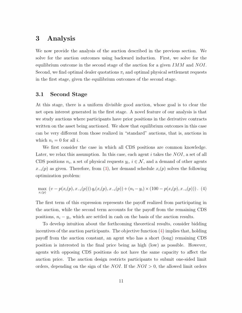
3 Analysis

We now provide the analysis of the auction described in the previous section. We

solve for the auction outcomes using backward induction. First, we solve for the

equilibrium outcome in the second stage of the auction for a given IMM and NOI.

Second, we find optimal dealer quotations πi and optimal physical settlement requests

in the first stage, given the equilibrium outcomes of the second stage.

3.1 Second Stage

At this stage, there is a uniform divisible good auction, whose goal is to clear the

net open interest generated in the first stage. A novel feature of our analysis is that

we study auctions where participants have prior positions in the derivative contracts

written on the asset being auctioned. We show that equilibrium outcomes in this case

can be very different from those realized in “standard” auctions, that is, auctions in

which ni = 0 for all i.

We first consider the case in which all CDS positions are common knowledge.

Later, we relax this assumption. In this case, each agent i takes the NOI, a set of all

CDS positions ni, a set of physical requests yi, i ∈ N , and a demand of other agents

x−i(p) as given. Therefore, from (3), her demand schedule xi(p) solves the following

optimization problem:

maxxi(p)

(v − p(xi(p), x−i(p))) qi(xi(p), x−i(p)) + (ni−yi)× (100− p(xi(p), x−i(p))) . (4)

The first term of this expression represents the payoff realized from participating in

the auction, while the second term accounts for the payoff from the remaining CDS

positions, ni − yi, which are settled in cash on the basis of the auction results.

To develop intuition about the forthcoming theoretical results, consider bidding

incentives of the auction participants. The objective function (4) implies that, holding

payoff from the auction constant, an agent who has a short (long) remaining CDS

position is interested in the final price being as high (low) as possible. However,

agents with opposing CDS positions do not have the same capacity to affect the

auction price. The auction design restricts participants to submit one-sided limit

orders, depending on the sign of the NOI. If the NOI > 0, the allowed limit orders

11

are to buy, and, therefore, agents with short CDS positions are capable of bidding

the price up. In contrast, the most agents with long CDS positions can do to bid the

price down is not to bid at all. The situation is reversed when the NOI < 0.

Continuing with the case of the NOI > 0, consider an example of only one agent

with a short CDS position. It is clear that she would be interested in bidding the

price as high as possible if the NOI is smaller than the notional amount of her CDS

(provided that she is allowed to hold defaulted bonds). This is because the cost of

purchasing bonds at a high auction price is offset by the benefit of cash-settling CDS

at the same high price. In contrast, if the NOI is larger than the notional amount of

her CDS position, she would not bid the price above the fair bond value v. This is

because the cost of purchasing bonds at a price above v is not offset by the benefit

of cash-settling CDS. We show in the sequel that this intuition can be generalized

to multiple agents as a long as we consider the size of their aggregate CDS positions

relative to the NOI.

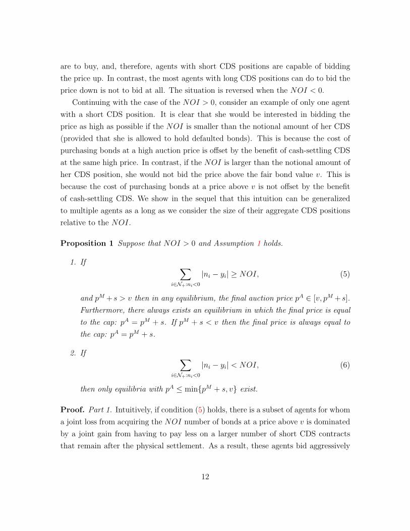
Proposition 1 Suppose that NOI > 0 and Assumption 1 holds.

1. If ∑i∈N+:ni<0

|ni − yi| ≥ NOI, (5)

and pM +s > v then in any equilibrium, the final auction price pA ∈ [v, pM +s].

Furthermore, there always exists an equilibrium in which the final price is equal

to the cap: pA = pM + s. If pM + s < v then the final price is always equal to

the cap: pA = pM + s.

2. If ∑i∈N+:ni<0

|ni − yi| < NOI, (6)

then only equilibria with pA ≤ min{pM + s, v} exist.

Proof. Part 1. Intuitively, if condition (5) holds, there is a subset of agents for whom

a joint loss from acquiring the NOI number of bonds at a price above v is dominated

by a joint gain from having to pay less on a larger number of short CDS contracts

that remain after the physical settlement. As a result, these agents bid aggressively

12

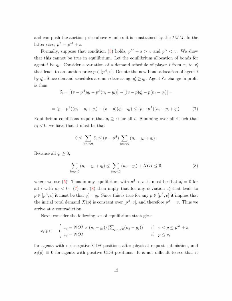
and can push the auction price above v unless it is constrained by the IMM. In the

latter case, pA = pM + s.

Formally, suppose that condition (5) holds, pM + s > v and pA < v. We show

that this cannot be true in equilibrium. Let the equilibrium allocation of bonds for

agent i be qi. Consider a variation of a demand schedule of player i from xi to x′i

that leads to an auction price p ∈ [pA, v]. Denote the new bond allocation of agent i

by q′i. Since demand schedules are non-decreasing, q′i ≥ qi. Agent i′s change in profit

is thus

δi =[(v − pA)qi − pA(ni − yi)

]− [(v − p)q′i − p(ni − yi)] =

= (p− pA)(ni − yi + qi)− (v − p)(q′i − qi) ≤ (p− pA)(ni − yi + qi). (7)

Equilibrium conditions require that δi ≥ 0 for all i. Summing over all i such that

ni < 0, we have that it must be that

0 ≤∑i:ni<0

δi ≤ (v − pA)∑i:ni<0

(ni − yi + qi) .

Because all qi ≥ 0,∑i:ni<0

(ni − yi + qi) ≤∑i:ni<0

(ni − yi) +NOI ≤ 0, (8)

where we use (5). Thus in any equilibrium with pA < v, it must be that δi = 0 for

all i with ni < 0. (7) and (8) then imply that for any deviation x′i that leads to

p ∈ [pA, v] it must be that q′i = qi. Since this is true for any p ∈ [pA, v] it implies that

the initial total demand X(p) is constant over [pA, v], and therefore pA = v. Thus we

arrive at a contradiction.

Next, consider the following set of equilibrium strategies:

xi(p) :

{xi = NOI × (ni − yi)/(

∑j:nj<0(nj − yj)) if v < p ≤ pM + s,

xi = NOI if p ≤ v,

for agents with net negative CDS positions after physical request submission, and

xi(p) ≡ 0 for agents with positive CDS positions. It is not difficult to see that it

13

supports pA = pM + s.

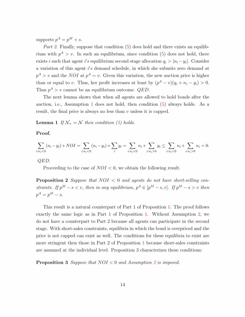
Part 2. Finally, suppose that condition (5) does hold and there exists an equilib-

rium with pA > v. In such an equilibrium, since condition (5) does not hold, there

exists i such that agent i′s equilibrium second stage allocation qi > |ni−yi|. Consider

a variation of this agent i′s demand schedule, in which she submits zero demand at

pA > v and the NOI at pA = v. Given this variation, the new auction price is higher

than or equal to v. Thus, her profit increases at least by (pA − v)(qi + ni − yi) > 0.

Thus pA > v cannot be an equilibrium outcome. QED.

The next lemma shows that when all agents are allowed to hold bonds after the

auction, i.e., Assumption 1 does not hold, then condition (5) always holds. As a

result, the final price is always no less than v unless it is capped.

Lemma 1 If N+ = N then condition (5) holds.

Proof.∑i:ni<0

(ni−yi)+NOI =∑i:ni<0

(ni−yi)+∑i

yi =∑i:ni<0

ni+∑i:ni>0

yi ≤∑i:ni<0

ni+∑i:ni>0

ni = 0.

QED.

Proceeding to the case of NOI < 0, we obtain the following result.

Proposition 2 Suppose that NOI < 0 and agents do not have short-selling con-

straints. If pM − s < v, then in any equilibrium, pA ∈ [pM − s, v]. If pM − s > v then

pA = pM − s.

This result is a natural counterpart of Part 1 of Proposition 1. The proof follows

exactly the same logic as in Part 1 of Proposition 1. Without Assumption 2, we

do not have a counterpart to Part 2 because all agents can participate in the second

stage. With short-sales constraints, equilibria in which the bond is overpriced and the

price is not capped can exist as well. The conditions for these equilibria to exist are

more stringent then those in Part 2 of Proposition 1 because short-sales constraints

are assumed at the individual level. Proposition 3 characterizes these conditions:

Proposition 3 Suppose that NOI < 0 and Assumption 2 is imposed.

14

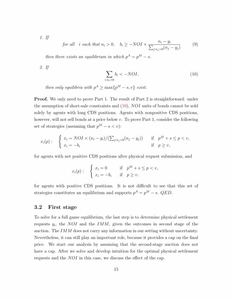
1. If

for all i such that ni > 0, bi ≥ −NOI ×ni − yi∑

j:nj>0(nj − yj)(9)

then there exists an equilibrium in which pA = pM − s.

2. If ∑i:ni>0

bi < −NOI, (10)

then only equilibria with pA ≥ max{pM − s, v} exist.

Proof. We only need to prove Part 1. The result of Part 2 is straightforward: under

the assumption of short-sale constraints and (10), NOI units of bonds cannot be sold

solely by agents with long CDS positions. Agents with nonpositive CDS positions,

however, will not sell bonds at a price below v. To prove Part 1, consider the following

set of strategies (assuming that pM − s < v):

xi(p) :

{xi = NOI × (ni − yi)/(

∑j:nj<0(nj − yj)) if pM + s ≤ p < v,

xi = −bi if p ≥ v,

for agents with net positive CDS positions after physical request submission, and

xi(p) :

{xi = 0 if pM + s ≤ p < v,

xi = −bi if p ≥ v.

for agents with positive CDS positions. It is not difficult to see that this set of

strategies constitutes an equilibrium and supports pA = pM − s. QED.

3.2 First stage

To solve for a full game equilibrium, the last step is to determine physical settlement

requests yi, the NOI and the IMM , given the outcomes in second stage of the

auction. The IMM does not carry any information in our setting without uncertainty.

Nevertheless, it can still play an important role, because it provides a cap on the final

price. We start our analysis by assuming that the second-stage auction does not

have a cap. After we solve and develop intuition for the optimal physical settlement

requests and the NOI in this case, we discuss the effect of the cap.

15

3.2.1 Second-Stage Auction without Cap

First, we show that in a frictionless world, only very particular equilibria with an

auction price different from v exist. Furthermore, in all these equilibria, agents receive

the same utility.

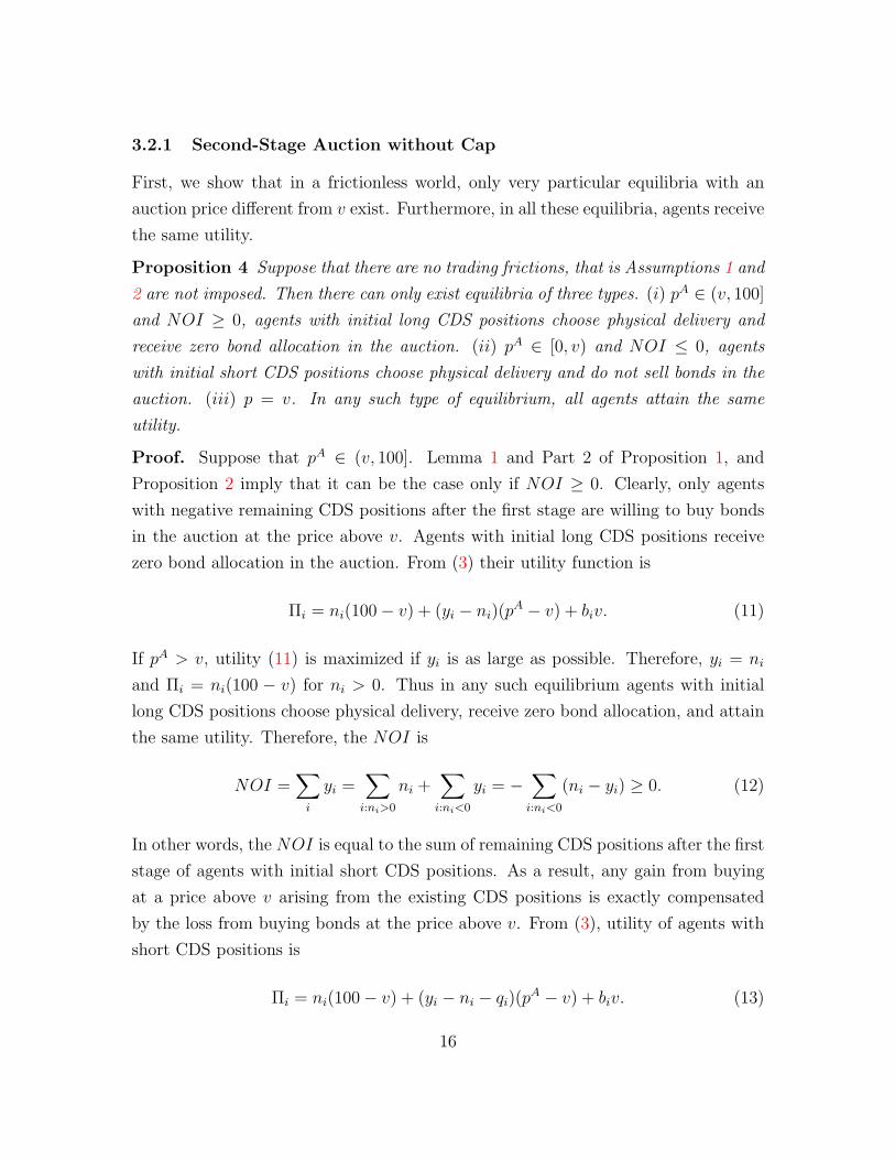
Proposition 4 Suppose that there are no trading frictions, that is Assumptions 1 and

2 are not imposed. Then there can only exist equilibria of three types. (i) pA ∈ (v, 100]

and NOI ≥ 0, agents with initial long CDS positions choose physical delivery and

receive zero bond allocation in the auction. (ii) pA ∈ [0, v) and NOI ≤ 0, agents

with initial short CDS positions choose physical delivery and do not sell bonds in the

auction. (iii) p = v. In any such type of equilibrium, all agents attain the same

utility.

Proof. Suppose that pA ∈ (v, 100]. Lemma 1 and Part 2 of Proposition 1, and

Proposition 2 imply that it can be the case only if NOI ≥ 0. Clearly, only agents

with negative remaining CDS positions after the first stage are willing to buy bonds

in the auction at the price above v. Agents with initial long CDS positions receive

zero bond allocation in the auction. From (3) their utility function is

Πi = ni(100− v) + (yi − ni)(pA − v) + biv. (11)

If pA > v, utility (11) is maximized if yi is as large as possible. Therefore, yi = ni

and Πi = ni(100 − v) for ni > 0. Thus in any such equilibrium agents with initial

long CDS positions choose physical delivery, receive zero bond allocation, and attain

the same utility. Therefore, the NOI is

NOI =∑i

yi =∑i:ni>0

ni +∑i:ni<0

yi = −∑i:ni<0

(ni − yi) ≥ 0. (12)

In other words, the NOI is equal to the sum of remaining CDS positions after the first

stage of agents with initial short CDS positions. As a result, any gain from buying

at a price above v arising from the existing CDS positions is exactly compensated

by the loss from buying bonds at the price above v. From (3), utility of agents with

short CDS positions is

Πi = ni(100− v) + (yi − ni − qi)(pA − v) + biv. (13)

16

Because every agent can always guarantee herself utility Πi = ni(100−v) by choosing

physical delivery, qi cannot be higher than −(ni − yi). Because of (12), qi cannot

be lower than −(ni − yi). Therefore, qi = −(ni − yi) and Πi = ni(100 − v) for each

i : ni < 0. The proof for the case of pA ∈ [0, v) is similar. QED.

Proposition 4 shows that in a frictionless world, all the mispricing equilibria are

unidirectional, that is, there is no under- (over-) pricing if the NOI is positive (neg-

ative). Furthermore, agents can undo any utility loss resulting from mispricing in an

auction by optimally choosing between cash and physical settlement of their positions.

We now turn to more realistic setups with trading frictions. Our analysis in section

3.1 shows that there can be a continuum of equilibria in the second stage, which

makes solving for all equilibria of a two-stage auction a daunting problem. Instead

of characterizing all the equilibria, we show that in the presence of trading frictions

outlined in Section 2.4, there exists a subset of equilibria of the two-stage game that

results in bond mispricing in the auction. This result answers affirmatively our main

question whether mispricing is possible in the auction. Proposition 5 characterizes

sufficient conditions for underpricing:

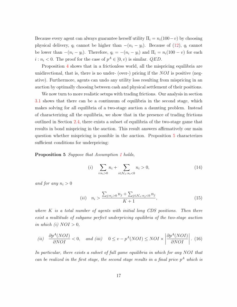
Proposition 5 Suppose that Assumption 1 holds,

(i)∑i:ni>0

ni +∑

i∈N+:ni<0

ni > 0, (14)

and for any ni > 0

(ii) ni >

∑j:nj>0 nj +

∑j∈N+:nj<0 nj

K + 1, (15)

where K is a total number of agents with initial long CDS positions. Then there

exist a multitude of subgame perfect underpricing equilibria of the two-stage auction

in which (i) NOI > 0,

(ii)∂pA(NOI)

∂NOI< 0, and (iii) 0 ≤ v− pA(NOI) ≤ NOI ×

∣∣∣∣∂pA(NOI)

∂NOI

∣∣∣∣ . (16)

In particular, there exists a subset of full game equilibria in which for any NOI that

can be realized in the first stage, the second stage results in a final price pA which is

17

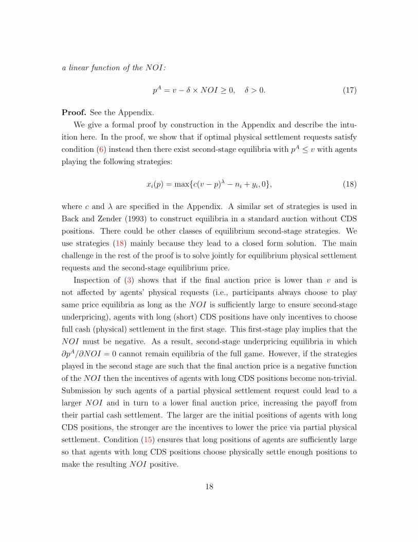
a linear function of the NOI:

pA = v − δ ×NOI ≥ 0, δ > 0. (17)

Proof. See the Appendix.

We give a formal proof by construction in the Appendix and describe the intu-

ition here. In the proof, we show that if optimal physical settlement requests satisfy

condition (6) instead then there exist second-stage equilibria with pA ≤ v with agents

playing the following strategies:

xi(p) = max{c(v − p)λ − ni + yi, 0}, (18)

where c and λ are specified in the Appendix. A similar set of strategies is used in

Back and Zender (1993) to construct equilibria in a standard auction without CDS

positions. There could be other classes of equilibrium second-stage strategies. We

use strategies (18) mainly because they lead to a closed form solution. The main

challenge in the rest of the proof is to solve jointly for equilibrium physical settlement

requests and the second-stage equilibrium price.

Inspection of (3) shows that if the final auction price is lower than v and is

not affected by agents’ physical requests (i.e., participants always choose to play

same price equilibria as long as the NOI is sufficiently large to ensure second-stage

underpricing), agents with long (short) CDS positions have only incentives to choose

full cash (physical) settlement in the first stage. This first-stage play implies that the

NOI must be negative. As a result, second-stage underpricing equilibria in which

∂pA/∂NOI = 0 cannot remain equilibria of the full game. However, if the strategies

played in the second stage are such that the final auction price is a negative function

of the NOI then the incentives of agents with long CDS positions become non-trivial.

Submission by such agents of a partial physical settlement request could lead to a

larger NOI and in turn to a lower final auction price, increasing the payoff from

their partial cash settlement. The larger are the initial positions of agents with long

CDS positions, the stronger are the incentives to lower the price via partial physical

settlement. Condition (15) ensures that long positions of agents are sufficiently large

so that agents with long CDS positions choose physically settle enough positions to

make the resulting NOI positive.

18

The subset of equilibria characterized in Proposition 5 is the simplest and serves as

an example of underpricing. There may be other equilibria resulting in underpricing

that we have not found. While Lemma 1 implies that condition (14) is necessary for

an underpricing equilibrium to exist, condition (15) can be relaxed at the expense of

a more complicated proof.

Finally, notice that if there are short-sale constraints, that is Assumption 2 is

imposed, then the logic of Proposition 4 may also break down. In this case, agents

with initial long CDS positions are able to choose only bi units of bonds for physical

settlement. Therefore, if at least for one such agent ni > bi and sufficiently many

agents with remaining short CDS positions participate, they could be strictly better

off as a group from pushing the price above v. Proposition 6 characterizes the effect

of short-sale constraints on auction outcomes:

Proposition 6 Suppose that only Assumption 2 is imposed and there exists i such

that

ni > bi > 0, (19)

and ∑j:nj<0

|nj| >∑j:nj>0

max{bj, 0}. (20)

Then there exist a subgame perfect overpricing equilibrium of the two-stage auction

in which NOI =∑

j:nj>0 max{bj, 0} > 0, pA = 100 and agents with initial short CDS

positions attain strictly larger utility compared to the one when pA = v.

Proof. The proof is by construction. As in Proposition 4, if pA = 100 agents who are

initially long CDS choose physical delivery, and only agents with negative remaining

CDS positions after the first stage are willing to buy bonds in the auction. Proposition

1 Part 1 shows that for any NOI > 0, if condition (5) holds (which turns out to be

the case in the constructed equilibrium) then pA = 100 is an equilibrium of the second

stage if agents use the following strategies:

xi(p) :

{xi = NOI × (ni − yi)/(

∑j:nj<0(nj − yj)) if v < p ≤ 100,

xi = NOI if p ≤ v.

19

for agents with net negative CDS positions after physical request submission, and

xi(p) ≡ 0 for other agents. The profit of an agent i with ni < 0 is therefore

Πi =

(yi −NOI

ni − yi∑j:nj<0(nj − yj)

)(100− v) + biv. (21)

Taking the F.O.C. at yi = 0 one can verify that it is optimal for agents with initial

short CDS positions to choose cash settlement. Thus NOI =∑

j:nj>0 max{bj, 0} and

for any agent i with initial short CDS position ni < 0, its profit is

Πi = −(100− v)ni ×∑

j:nj>0 max{bj, 0}∑j:nj<0 nj

+ biv > (100− v)ni + biv,

where the right hand side expression is the agent’s utility if pA is equal to v. QED.

Propositions 5 and 6 show that if there are trading frictions then there can be

either underpricing or overpricing equilibria with NOI > 0 in the two-stage game. A

similar set of results can be obtained with NOI < 0.

3.2.2 Second-Stage Auction with Cap

Now we discuss how the presence of the second-stage cap affects our analysis. The

cap restricts the final price to be no higher than pM + s. Therefore, in the presence

of the cap, mispricing in the auction depends on the bidding behavior of dealers in

the first stage. The next proposition shows that the IMM is equal to v when there

are no trading frictions.

Proposition 7 Suppose that there are no trading frictions, that is Assumptions 1

and 2 are not imposed, and γ > 0. Then IMM = v. Therefore, of the overpricing

equilibria described in Proposition 4 there can exist only equilibria with |pA − v| ≤ s.

Proof. Proposition 4 shows that in all possible equilibria, common participants

attain the same utility. Because dealers have regulatory and reputational concerns,

captured by the extra term −γ(πi − v)2, their optimal quotes, πi, are equal to v.

Thus, IMM = v. QED.

20

This result further restricts a set of possible full game equilibria. The final action

price cannot be different from the fair value by more than the size of the spread, s

when there are no frictions.

In the presence of frictions, there can be either underpricing or overpricing equi-

libria in the auction without cap (Propositions 5 and 6). The presence of the cap

cannot eliminate underpricing equilibria.4 Additionally, the cap, if it is set too low,

rules out equilibria with pA = v.

The cap can be effective at eliminating overpricing equilibria. To illustrate, con-

sider a simple example in which all dealers have zero CDS positions.5 Proposition 6

shows that when there are short-sale constraints, in the absence of the cap, the final

auction price can be as high as 100. Following the same logic as in Proposition 6 one

can show that, if there is a cap that is greater than v, then there exists an equilib-

rium with the final price equal to the cap. Because in any such equilibrium dealers do

not realize any profit but have regulatory and reputational concerns dealers’ optimal

quotes are equal to v. Thus, IMM = v and pA = v + s.

4 Empirical Evidence

Our theoretical analysis shows that the CDS auctions may result in both overpric-

ing and underpricing of the underlying bonds. In this section, we seek to establish

evidence regarding which outcomes are realised in practice. Unfortunately, the true

value of deliverable bonds is not observed. Because of this, in our empirical analysis,

we use available bond prices from the day before an auction to construct a proxy for

the bond value v. Admittedly, this measure is not a perfect substitute for the true

value of the bond. Therefore, later we consider a number of alternatives to show the

robustness of our results. We first describe our data and then present the empirical

analysis.

4For example, consider an extreme case, in which all dealers have large positive CDS positionsand conditions of Proposition 5 hold. Following the logic of Proposition 5 one can show that thereexists a subgame perfect equilibrium in which pA = 0 and IMM = v.

5This case is a simplification but is arguably realistic as dealers try to maintain zero CDS positionsin their market-making capacity.

21

4.1 Data

Our data come from two primary sources. The details of the auction settlement

are publicly available from the Creditfixings website (www.creditfixings.com). As

of December 2010, there have been 86 CDS and Loan CDS auctions, which settle

contracts on both US and international legal entities. To study the relationship

between auction outcomes and bond values, we merge these data with the bond price

data from the TRACE database. TRACE reports corporate bond trades for US

companies only. Thus, our merged dataset contains 23 auctions.

Table 2 summarizes the results of the auctions for these firms. It reports a settle-

ment date, a type of credit event, and auction outcomes. Most of the auctions took

place in 2009 and were triggered by the Chapter 11 event. Of the 23 auctions, only

two (Six Flags and General Motors) have the net open interest to buy (NOI < 0).

The full universe of CDS auctions contains 61 auctions that have the net open interest

to sell, 19 auctions that have the net open interest to buy, and 6 auctions that have

zero net open interest.

Table 3 provides summary statistics of deliverable bonds for each auction for which

we have the bond data.6 Deliverable bonds are reported in auction protocols, which

are available from the Creditfixings website. The table also reports the ratio of the

net open interest to the notional amount of deliverable bonds (NOI/NAB). It shows

how many bonds change hands during the auction as a percentage of the total amount

of bonds. There is strong heterogeneity in NOI/NAB across different auctions. The

absolute value ranges from 0.38% to 56.81%. In practice, NOI has never exceeded

NAB.

We construct daily bond prices by weighing the price corresponding to each trade

against the trade size reported in TRACE as in Bessembinder, Kahle, Maxwell, and

Xuet (2009). These authors advocate eliminating all trades under $100,000 because

they are likely to be noninstitutional. The larger trades have lower execution costs;

hence, they should reflect the underlying bond value with greater precision. For each

6A clarification regarding the auctions of Abitibi and Bowater is in order. AbitibiBowater isa corporation, formed by Abitibi and Bowater for the sole purpose of effecting their combination.Upon completion of the combination, Abitibi and Bowater became subsidiaries of AbitibiBowaterand the business of AbitibiBowater are the businesses that used to be conducted by Abitibi andBowater. The CDS contracts were linked to the entities separately, and, as a result, there were twoseparate auctions.

22

company, we build a time-series of bond prices in the auction event window of -30 to

+30 trading days. Because all credit events occurred within a calendar month of the

CDS auction, our choice of the event window ensures that our sample contains all the

data for the post-credit-event prices. The last column of Table 3, reports a weighted

average bond price on the day before the auction, p−1. We use it as a proxy for the

bond value v.

4.2 The Impact of the First Stage

The theoretical results of Section 3 imply that the first and the second stages of the

auction are not independent. The first stage yields the mid-point price, pM , which

determines a cap on the final settlement price. Our model shows that when the final

price, pA, is capped, it can be either above or below the true value of the bond, v,

depending on the initial CDS and bond positions of different agents.

Our analysis suggests a way of differentiating between the two cases. Specifically,

consider outcomes in which NOI > 0 (outcomes in which NOI < 0 follow similar

logic). According to Proposition 1 Part 1, the price can be higher than v if the

aggregate short CDS position after the first stage of the agents who participate in

the second stage is larger than the net open interest. In this case, agents who sold

protection have an incentive to bid above the true value of the bond to minimize the

amount paid to a CDS counterparty. Notice that while bidding at the price above

v, they would like to minimize the amount of bonds acquired at the auction for a

given final auction price. Thus, they would never bid to buy more than NOI units

of bonds at prices above v.

The case in which pA is capped and is below the true value of the bond is realized

when the dealers set pM so that pM + s is below v. Doing so prevents the agents

from playing second-stage equilibria with the final price above the cap. In this case,

submitting a large demand at a cap price leads to a greater profit. Thus, in the

presence of competition and sharing rules, agents have an incentive to buy as many

bonds as possible. Thus, they would bid to buy substantially more than NOI units.

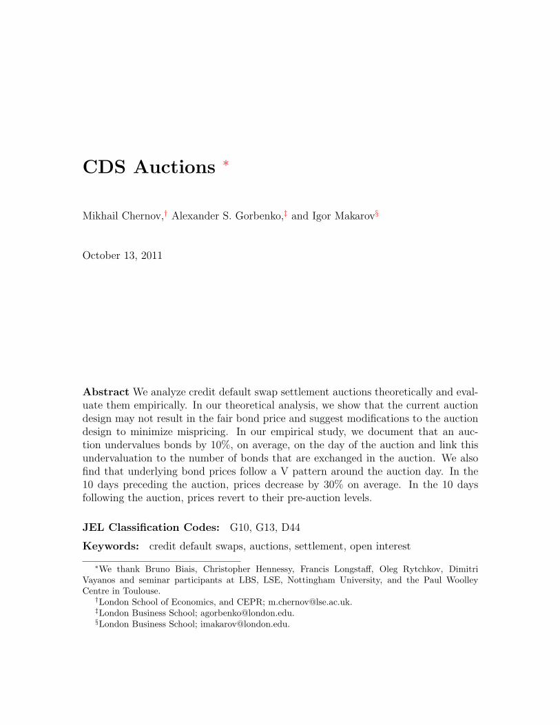
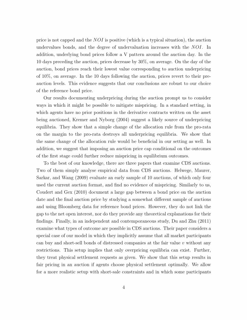
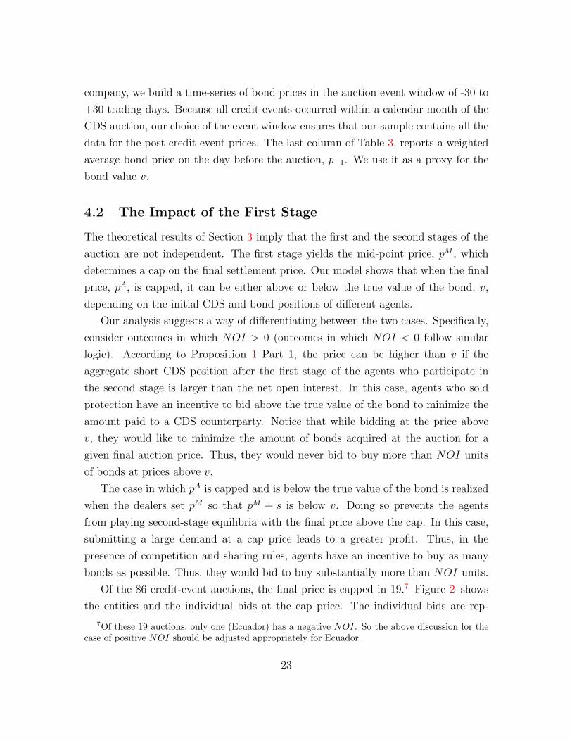
Of the 86 credit-event auctions, the final price is capped in 19.7 Figure 2 shows

the entities and the individual bids at the cap price. The individual bids are rep-

7Of these 19 auctions, only one (Ecuador) has a negative NOI. So the above discussion for thecase of positive NOI should be adjusted appropriately for Ecuador.

23

resented by different colors. The bid sizes are scaled by NOI to streamline the

interpretation. For example, in total, there are seven bids at the cap price in the case

of General Growth Properties. Six of them are equal to NOI and the seventh one is

approximately one-fourth of NOI.

We can see that in all but two auctions (Kaupthing Bank and Glitnir), the bids at

the price cap do not exceed NOI. These results suggest in these cases, the final auc-

tion price is above the true bond value. Of the 19 auctions with capped price, we have

bond data for only five companies: Smurfit-Stone, Rouse, Charter Communications,

Capmark, Bowater. Comparing the final action price from Table 2 with the bond

price from Table 3 we can see that that, as anticipated, the bond price (our proxy for

the true bond value) is below the final auction price for these five companies.

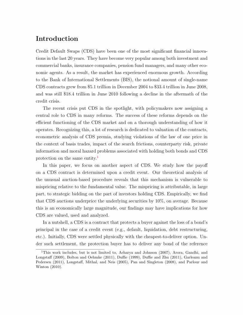
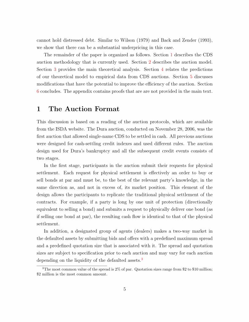
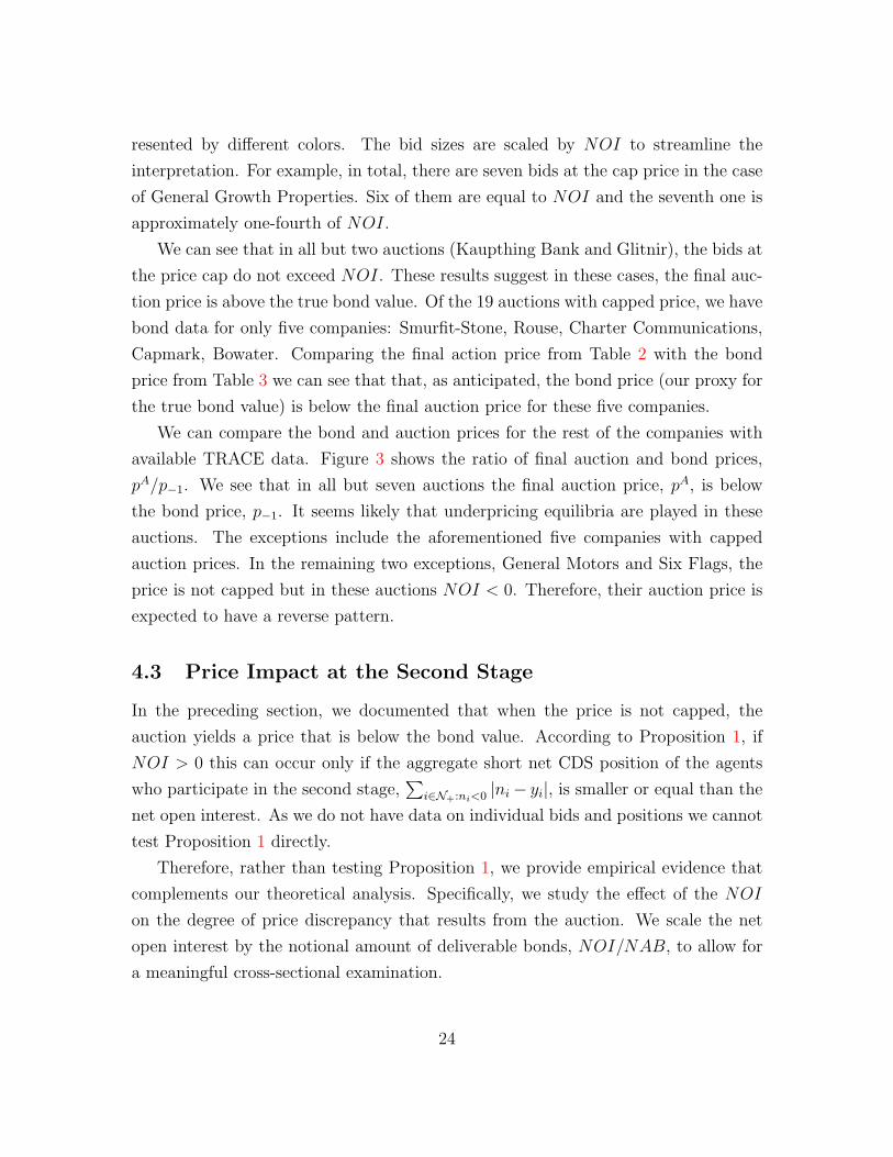
We can compare the bond and auction prices for the rest of the companies with

available TRACE data. Figure 3 shows the ratio of final auction and bond prices,

pA/p−1. We see that in all but seven auctions the final auction price, pA, is below

the bond price, p−1. It seems likely that underpricing equilibria are played in these

auctions. The exceptions include the aforementioned five companies with capped

auction prices. In the remaining two exceptions, General Motors and Six Flags, the

price is not capped but in these auctions NOI < 0. Therefore, their auction price is

expected to have a reverse pattern.

4.3 Price Impact at the Second Stage

In the preceding section, we documented that when the price is not capped, the

auction yields a price that is below the bond value. According to Proposition 1, if

NOI > 0 this can occur only if the aggregate short net CDS position of the agents

who participate in the second stage,∑

i∈N+:ni<0 |ni− yi|, is smaller or equal than the

net open interest. As we do not have data on individual bids and positions we cannot

test Proposition 1 directly.

Therefore, rather than testing Proposition 1, we provide empirical evidence that

complements our theoretical analysis. Specifically, we study the effect of the NOI

on the degree of price discrepancy that results from the auction. We scale the net

open interest by the notional amount of deliverable bonds, NOI/NAB, to allow for

a meaningful cross-sectional examination.

24

Tables 2 and 3 reveal that NOI/NAB has the largest values in the auctions where

the largest discrepancy in prices occurs. At the same time, NOI/NAB has the lowest

values in the auctions where the final price is capped, which is again consistent with

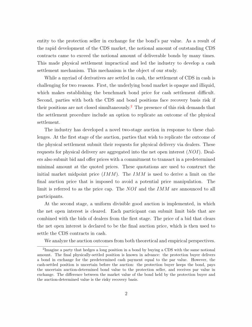
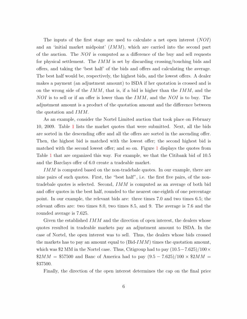
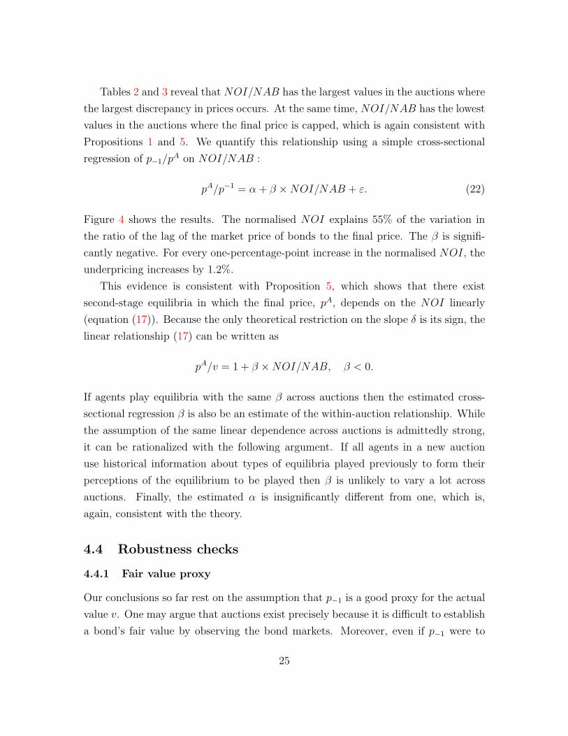
Propositions 1 and 5. We quantify this relationship using a simple cross-sectional

regression of p−1/pA on NOI/NAB :

pA/p−1 = α + β ×NOI/NAB + ε. (22)

Figure 4 shows the results. The normalised NOI explains 55% of the variation in

the ratio of the lag of the market price of bonds to the final price. The β is signifi-

cantly negative. For every one-percentage-point increase in the normalised NOI, the

underpricing increases by 1.2%.

This evidence is consistent with Proposition 5, which shows that there exist

second-stage equilibria in which the final price, pA, depends on the NOI linearly

(equation (17)). Because the only theoretical restriction on the slope δ is its sign, the

linear relationship (17) can be written as

pA/v = 1 + β ×NOI/NAB, β < 0.

If agents play equilibria with the same β across auctions then the estimated cross-

sectional regression β is also be an estimate of the within-auction relationship. While

the assumption of the same linear dependence across auctions is admittedly strong,

it can be rationalized with the following argument. If all agents in a new auction

use historical information about types of equilibria played previously to form their

perceptions of the equilibrium to be played then β is unlikely to vary a lot across

auctions. Finally, the estimated α is insignificantly different from one, which is,

again, consistent with the theory.

4.4 Robustness checks

4.4.1 Fair value proxy

Our conclusions so far rest on the assumption that p−1 is a good proxy for the actual

value v. One may argue that auctions exist precisely because it is difficult to establish

a bond’s fair value by observing the bond markets. Moreover, even if p−1 were to

25

reflect the bond value accurately, it would the value on the day before the auction.

It is conceivable that the auction process establishes the correct value v that differs

from p−1 simply because of the arrival of new information between time −1 and 0

and/or because of the centralised clearing mechanism of the auction.

We expand the auction event window to check robustness of our results to these

caveats. The shortest time between a credit event and an auction is 8 days in our

sample. This prompts us to select an event window of -8 to +12 days. The choice

of the right boundary is dictated by considerations of liquidity: liquidity generally

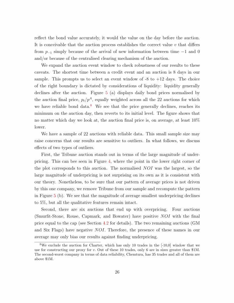
declines after the auction. Figure 5 (a) displays daily bond prices normalised by

the auction final price, pt/pA, equally weighted across all the 22 auctions for which

we have reliable bond data.8 We see that the price generally declines, reaches its

minimum on the auction day, then reverts to its initial level. The figure shows that

no matter which day we look at, the auction final price is, on average, at least 10%

lower.

We have a sample of 22 auctions with reliable data. This small sample size may

raise concerns that our results are sensitive to outliers. In what follows, we discuss

effects of two types of outliers.

First, the Tribune auction stands out in terms of the large magnitude of under-

pricing. This can bee seen in Figure 4, where the point in the lower right corner of

the plot corresponds to this auction. The normalised NOI was the largest, so the

large magnitude of underpricing is not surprising on its own as it is consistent with

our theory. Nonetheless, to be sure that our pattern of average prices is not driven

by this one company, we remove Tribune from our sample and recompute the pattern

in Figure 5 (b). We see that the magnitude of average smallest underpricing declines

to 5%, but all the qualitative features remain intact.

Second, there are six auctions that end up with overpricing. Four auctions

(Smurfit-Stone, Rouse, Capmark, and Bowater) have positive NOI with the final

price equal to the cap (see Section 4.2 for details). The two remaining auctions (GM

and Six Flags) have negative NOI. Therefore, the presence of these names in our

average may only bias our results against finding underpricing.

8We exclude the auction for Charter, which has only 10 trades in the [-10,0] window that weuse for constructing our proxy for v. Out of these 10 trades, only 6 are in sizes greater than $1M.The second-worst company in terms of data reliability, Chemtura, has 35 trades and all of them areabove $1M.

26

The documented V shape of the discrepancy alleviates the concern that the correct

value v differs from p−1 simply because the latter does not reflect the bond value

correctly. If it were the case, one would expect bond prices to hover around the

auction price after the auction. In practice, bond prices increase after the auction.

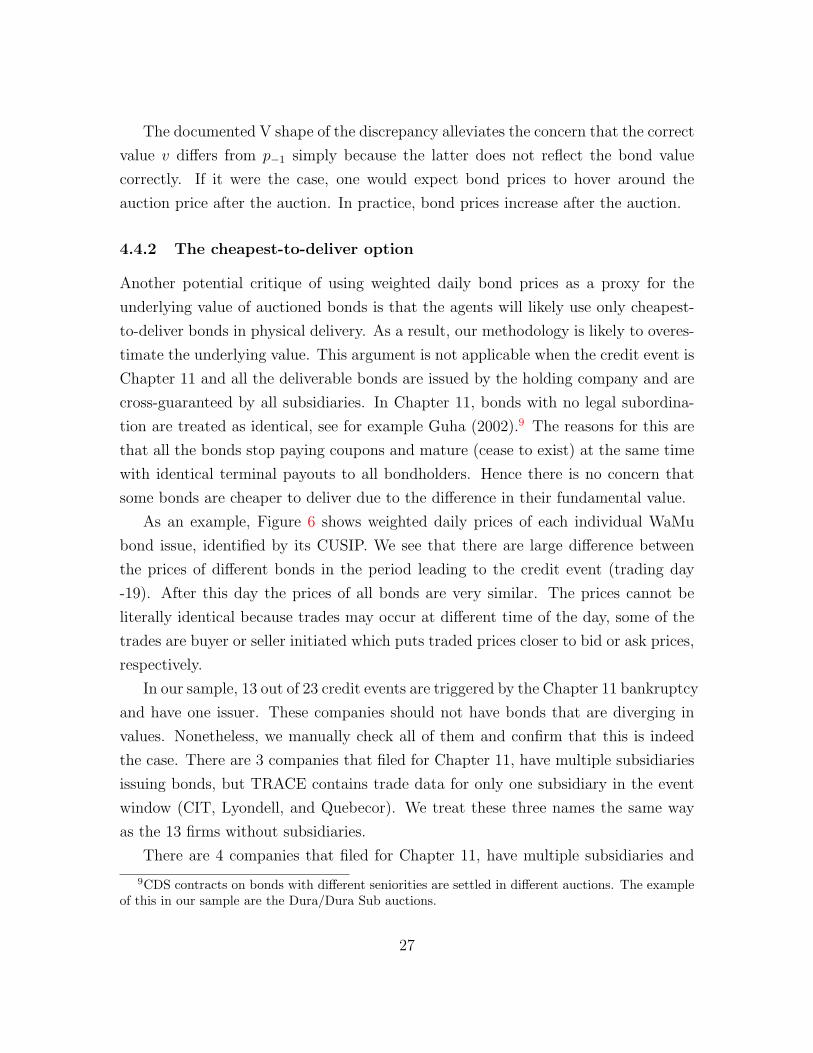
4.4.2 The cheapest-to-deliver option

Another potential critique of using weighted daily bond prices as a proxy for the

underlying value of auctioned bonds is that the agents will likely use only cheapest-

to-deliver bonds in physical delivery. As a result, our methodology is likely to overes-

timate the underlying value. This argument is not applicable when the credit event is

Chapter 11 and all the deliverable bonds are issued by the holding company and are

cross-guaranteed by all subsidiaries. In Chapter 11, bonds with no legal subordina-

tion are treated as identical, see for example Guha (2002).9 The reasons for this are

that all the bonds stop paying coupons and mature (cease to exist) at the same time

with identical terminal payouts to all bondholders. Hence there is no concern that

some bonds are cheaper to deliver due to the difference in their fundamental value.

As an example, Figure 6 shows weighted daily prices of each individual WaMu

bond issue, identified by its CUSIP. We see that there are large difference between

the prices of different bonds in the period leading to the credit event (trading day

-19). After this day the prices of all bonds are very similar. The prices cannot be

literally identical because trades may occur at different time of the day, some of the

trades are buyer or seller initiated which puts traded prices closer to bid or ask prices,

respectively.

In our sample, 13 out of 23 credit events are triggered by the Chapter 11 bankruptcy

and have one issuer. These companies should not have bonds that are diverging in

values. Nonetheless, we manually check all of them and confirm that this is indeed

the case. There are 3 companies that filed for Chapter 11, have multiple subsidiaries

issuing bonds, but TRACE contains trade data for only one subsidiary in the event

window (CIT, Lyondell, and Quebecor). We treat these three names the same way

as the 13 firms without subsidiaries.

There are 4 companies that filed for Chapter 11, have multiple subsidiaries and

9CDS contracts on bonds with different seniorities are settled in different auctions. The exampleof this in our sample are the Dura/Dura Sub auctions.

27

we have data for the bonds of these subsidiaries (Bowater, Charter, Nortel, and

Smurfit-Stone). In all of these cases the bonds of the different subsidiaries are legally

pari-passu with each other, but some of them may be structurally subordinated to

others and, therefore, could be cheaper. For this reason, we select the cheaper bonds

in the case of these four companies (however, the differences are not large in practice).

There are 3 companies with a credit event other than Chapter 11 (Abitibi, Capmark,

and Rouse) in which we select the cheapest bonds as well.

Finally, to account for any other potential deliverables selection that could work

against our findings we treat the aforementioned differences in bond prices that are

due to bid-ask spread and different timing as real differences and select the lowest

priced bonds. Specifically, we take representative daily prices of company’s deliverable

bonds to be equal to weighted daily prices of their bond issues with the lowest pre-

auction price, provided that these bond issues are relatively actively traded.10 The

results are displayed in Figure 5. It can be seen that even with such conservative

bond selection, the average underpricing on the day of the auction is still 10% and

follows a V pattern.

5 Extensions

The empirical section documents that when NOI/NAB is large, the auction generally

results in a price that is considerably below the bond value. We now suggest several

modifications to the auction design that can reduce mispricing in auction outcomes

and discuss some of the assumptions of the model.

5.1 Allocation rule at the second stage

As usual, we focus on the case of NOI > 0. Proposition 1 shows that if condition (6)

holds, the CDS auction is similar to a “standard” auction, so the price can be below

v. Kremer and Nyborg (2004) show that in a setting without CDS positions, a simple

change of the allocation rule from pro rata on the margin rule (2) to the pro-rata rule

destroys all underpricing equilibria so that only pA = v remains. Under the pro-rata

10The requirement is that the trading volume over the final 5 trading days before the auctionconstitutes at least 5% of the total trading volume for the company

28

rule, the equilibrium allocations qi are given by

qi(pA) =

xi(pA)

X(pA)×NOI,

that is the total rather than marginal demand at pA is rationed among agents. The

next proposition extends the result of Kremer and Nyborg (2004) to our setting. We

demonstrate that if pM + s ≥ v, then second-stage equilibrium price pA cannot be

less than v. This is true even if the agents are allowed to hold non-zero quantities of

CDS contracts.

Proposition 8 Suppose that the auction sharing rule is pro-rata. Then, if NOI > 0

then pA ≥ min{pM + s, v}. If NOI < 0 then pA ≤ max{pM − s, v}.

Proof. See the Appendix.

Consider the case of the positive NOI to develop intuition for this result. Accord-

ing to Proposition 1 Part 2, if condition (6) holds then the pro-rata on the margin

allocation rule may inhibit competition and lead to underpricing equilibria. The pres-

ence of agents who are short CDS contracts does not help in this case. The pro-rata

allocation rule (i) does not guarantee the agents their inframarginal demand above

the clearing price and (ii) closely ties the proportion of allocated bonds to the ratio

of individual to total demand at the clearing price. Therefore, a switch to such a rule

increases competition for bonds among agents. As a result, even agents with long

positions bid aggressively. If pA < v then demanding the NOI at a price only slightly

higher than pA allows an agent to capture at least half of the surplus. As a result,

only fair-price equilibria survive.

5.2 The price cap

Our theoretical analysis in Section 4.2 shows that the presence of the cap can result

in either lower or larger mispricing in auction outcomes. The cap is likely to help

when |NOI| is small and the temptation to manipulate the auction results is highest.

At the same time, the cap allows dealers to limit the final price below v in the second

stage.

29

These results suggest that making the cap conditional on the outcome of the

first stage of a CDS auction can lead to a better auction design. In our base model

without uncertainty, the optimal conditional cap is trivial. Again, we consider the

case of NOI > 0. If pM < v, setting s∗ = v− pM ensures that the set of second-stage

equilibria includes v. If pM ≥ v, it is best to set s∗ = 0. While the conditional cap

cannot eliminate the worst underpricing equilibria it can ensure that the agents who

want to bid aggressively will be able to do so.

In practice, v and ni are unobservable. In this case, making the cap conditional

on NOI and on the ratio pM/p−1 could lead to the final auction price being closer to

the fair bond value. For example, if pM/p−1 ≤ α and the NOI is large, where α < 1

is reasonably small, the auctioneer can set a larger cap; if pM/p−1 > α and the NOI

is small, a smaller cap can be set.

5.3 Risk-averse agents

So far, we have restricted our attention to the setting with risk-neutral agents. This

allowed us to abstract from risk considerations. If agents are risk-averse, the reference

entity’s risk is generally priced. Even though a CDS is in a zero net supply, its

settlement leads to a reallocation of risk among the participants in the auction; hence,

it can lead to a different equilibrium bond price. In a particular scenario, when

NOI/NAB is large and positive and there are only a few risk-averse agents willing to

hold defaulted bonds, the auction results in a highly-concentrated ownership of the

company’s risk; hence, it can lead to a lower new equilibrium bond price.

Notice, however, that risk-aversion does not automatically imply a lower auction

price. For example, if marginal buyers of bonds in the auction are agents who pre-

viously had large negative CDS positions, as in Proposition 5, their risk exposure

after the auction may actually decrease. As a result they could command a lower risk

premium.

Due to the fact that we do not have data on individual agents’ bids and positions,

we cannot determine whether the observed price discrepancy is due to the mispricing

equilibria played or the risk-aversion channel. It is likely that both factors work

together in the same direction. Data on individual agents’ bids and positions could

help to quantify the effect of the two factors on the observed relationship between the

30

auction price and the size of the net open interest.

5.4 Private information

So far, we have restricted our attention to the simplest case in which agents’ CDS

positions are common knowledge. This may seem like a very strong assumption given

that CDS contracts are traded in the OTC market. Notice, however, that in the

type of equilibria constructed in Propositions 5 (linear case) and 6, conditions (14),

(15) and (19), (20) completely define the two equilibria. Therefore, Propositions 5

and 6 continue to hold with private CDS positions as long as (14), (15) and (19),

(20) are public knowledge.11 One can argue that this is likely to be the case. For

example, (20) assumes that the total short CDS positions are larger than the total

bond holdings of agents with long CDS positions. The aggregate net CDS positions

are known to market participants.12 Therefore, whether condition (20) holds can be

easily verified in every auction. Similarly, (19) assumes that there is an agent whose

long positions in CDS is larger than her bond holdings. Given the much larger size

of CDS contracts compared to the amount of bonds outstanding, (19) holds as long

the aggregate long CDS positions are larger than the amount of bonds outstanding.

The later is true for most (if not all) of the auctions.

We also assume that the agents have identical valuation of bonds and it is a

common knowledge. This assumption provides a stark benchmark: we are able to

show that the auction results in mispricing even in such a basic case. We conjecture

that it would be even harder for the current auction mechanism to yield the fair value

when agents have private or heterogeneous valuations.

6 Conclusion

We have presented a theoretical and empirical analysis of how CDS contracts are

settled when a credit event takes place. A two-stage auction-based procedure aims to

establish a reference bond price for cash settlement and to provide market participants

with an option to replicate an outcome of a physical settlement. The first stage

11The formal proofs follow closely the original proofs for the full information case and are availableupon request.

12For example, they are available from Markit reports.

31

determines the net open interest (NOI) in the physical settlement and the auction

price cap (minimum or maximum price depending on whether the NOI is to sell or to

buy). The second stage is a uniform divisible good auction with a marginal pro-rata

allocation rule that establishes the final price by clearing the NOI.

In our theoretical analysis, we show that the auction may result in either overpric-

ing or underpricing of the underlying bonds. Our empirical analysis establishes that

the former case is more prevalent. Bonds are underpriced by 10%, on average, and

the amount of underpricing is increasing with the NOI normalised by the notional

amount of deliverable bonds. We propose introducing a pro-rata allocation rule and

a conditional price cap to mitigate the mispricing.

32

References

[1] Viral Acharya and Timothy Johnson, 2007. “Insider Trading in Credit Deriva-

tives,” Journal of Financial Economics, vol. 84(1), pages 110-141.

[2] Navneet Arora, Priyank Gandhi, and Francis A. Longstaff, 2009. “Counterparty

Credit Risk and the Credit Default Swap Market,” working paper, UCLA

[3] Kerry Back and Jaime F. Zender, 1993. “Auctions of Divisible Goods: On the

Rationale for the Treasury Experiment,” Review of Financial Studies, vol. 6(4),

pages 733-764.

[4] Hendrik Bessembinder, Kathleen M. Kahle, William F. Maxwell, and Danielle

Xu, 2009. “Measuring Abnormal Bond Performance,” Review of Financial Stud-

ies, vol. 22(10), pages 4219-4258.

[5] Patrick Bolton and Martin Oehmke, 2011. “Credit Default Swaps and the Empty

Creditor Problem,” Review of Financial Studies, forthcoming

[6] Virginie Coudert and Mathieu Gex, 2010. “The Credit Default Swap Market and

the Settlement of Large Defaults,” working paper no. 2010-17, CEPII

[7] Songzi Du and Haoxiang Zhu, 2011. “Are CDS Auctions Biased?” working paper,

Stanford GSB

[8] Durrell Duffie, 1999. “Credit Swap Valuation,” Financial Analysts Journal,

January-February, pages 73-87.

[9] Durrell Duffie and Haoxiang Zhu, 2011. “Does a Central Clearing Counterparty

Reduce Counterparty Risk?” Review of Asset Pricing Studies, forthcoming.

[10] Nicolae Garleanu and Lasse Pedersen, 2011. “Margin-Based Asset Pricing and

Deviations from the Law of One Price,” Review of Financial Studies, forthcom-

ing.

[11] Rajiv Guha, 2002. “Recovery of Face Value at Default: Theory and Empirical

Evidence,” working paper, LBS.

33

[12] Jean Helwege, Samuel Maurer, Asani Sarkar, and Yuan Wang, 2009. “Credit

Default Swap Auctions and Price Discovery,” Journal of Fixed Income, Fall 2009,

pages 34-42.

[13] Ilan Kremer and Kjell G. Nyborg, 2004. “Divisible-Good Auctions: The Role of

Allocation Rules,” RAND Journal of Economics, vol. 35(1), pages 147-159.

[14] Francis A. Longstaff, Sanjay Mithal and Eric Neis, 2005. “Corporate Yield

Spreads: Default Risk or Liquity? New Evidence from the Credit-Default Swap

Market,” Journal of Finance, vol. 60, pages 2213-2253.

[15] Jun Pan and Kenneth Singleton, 2008. “Default and Recovery Implicit in the

Term Structure of Sovereign CDS Spreads,” Journal of Finance, vol. 63, pages

2345-2384.

[16] Christine Parlour and Andrew Winton, 2010. “Laying Off Credit Risk: Loan

Sales and Credit Default Swaps,” working paper, UC Berkeley

[17] Robert Wilson, 1979. “Auctions of Shares,” Quarterly Journal of Economics, vol.

93(4), pages 675-689.

34

Appendix

Proof of Proposition 5

The proof is by construction. We construct a subgame perfect two-stage equilibrium

in which the final auction price is a decreasing function of the NOI. Similar to

Kremer and Nyborg (2004), one can show that one can restrict his attention w.l.o.g.

to equilibria in differentiable strategies. For simplicity, we provide the proof for the

case in which agents have large long CDS positions. Specifically, we assume that for

all i : ni > 0 :

ni ≥ NOI. (A1)

Under this additional assumption, we can solve for the equilibrium in closed-form. A

general case follows similar logic. The main complication that arises in the general

case is that the number of the agents who submit nonzero demand for bonds at the

second stage depends on the configuration of CDS positions. When A1 holds, only

agents with nonpositive CDS positions receive nonzero allocations in the equilibrium.

The proof consists of several steps. In step 1, we derive the F.O.C. for the optimal

strategies at the second stage, given agents remaining CDS positions after the first

stage. In step 2, we derive the F.O.C. for the optimal physical settlement requests.

In step 3, we show that the second-stage equilibrium with price, pA, can be supported

if agents play the following strategies at the second stage:

xi(p) = max{c(v − p)λ − ni + yi, 0},

where c and λ are specified later. In step 4, we solve for optimal physical requests of

agents, given the above second-stage strategies. Finally, we solve for the NOI.

Step 1. Recall that at the second stage, a player i solves problem (4):

maxxi(p)

(v − p(xi(p), x−i(p))) qi(xi(p), x−i(p)) + (ni − yi)× (100− p(xi(p), x−i(p))) .

In any equilibrium of the second stage, the sum of the demand of an agent i, xi(pA)

and the residual demand of other players, x−i(pA) has to equal to the NOI. Therefore,

solving for the optimal xi(p) is equivalent to solving for the optimal price, pA, given

residual demand of other players. Thus, the F.O.C. for an agent i at the equilibrium

35

price, pA, can be written as

(v − pA)∂x−i(p

A)

∂p+ xi(p

A) + ni − yi = 0 if xi(pA) > 0, (A2)

(v − pA)∂x−i(p

A)

∂p+ xi(p

A) + ni − yi ≥ 0 if xi(pA) = 0. (A3)

Step 2. Recall that an agent i′s profit is given by equation (3):

Πi = (v − pA)qiauction-allocated bonds

+ (ni − yi)× (100− pA)remaining CDS

+ 100yiphysical settlement

+ v(bi − yi)remaining bonds

.

Using that ∂NOI/∂yi = 1 we have that the F.O.C. for the optimal settlement amount,

yi, for agent i satisfies

∂Πi

∂yi= 0 if yi 6= 0 and yi 6= ni, (A4)

∂Πi

∂yi≤ 0 if yi = 0 and ni > 0, or yi = ni if ni < 0, (A5)

∂Πi

∂yi≥ 0 if yi = 0 and ni < 0, or yi = ni if ni > 0, (A6)

where

∂Πi

∂yi= −∂p

A(NOI)

∂NOI(ni − yi + qi)− (v − pA(NOI))

(1− ∂qi

∂yi

). (A7)

Step 3. Let M be the number of the agents with nonpositive CDS positions who are

allowed to hold bonds and let λ = 1/(M −1). Consider the following set of strategies

at the second stage:

xi(p) = max

{NOI +

∑j∈N+:nj<0 (nj − yj)M

(v − p)λ

(v − pA(NOI))λ− ni + yi, 0

}. (A8)

Demand schedules (A8) imply that agents with the nonpositive CDS positions

36

who are allowed to hold bonds receive at p = pA the following bond allocations:

qi =NOI +

∑j∈N+:nj<0 (nj − yj)M

− (ni − yi). (A9)

Equation (A3) imply that agents with initial long CDS positions receive zero equilib-

rium bond allocations at the second stage as long as

ni − yi ≥NOI +

∑j∈N+:nj<0 (nj − yj)M − 1

. (A10)

If this is the case, equations (A2) imply that strategies (A8) form an equilibrium at

the second stage, with the equilibrium price equal to pA.13

Step 4. Consider now optimal physical requests of agents with initial short CDS

positions. We need to consider only those agents who are allowed to hold bonds after

the auction. In the equilibrium we construct in step 3, these agents receive qi units

of bonds given in (A9). So we can write condition (A7) as

∂Πi

∂yi= −∂p

A(NOI)

∂NOI

NOI +∑

j∈N+:nj<0 (nj − yj)M

− v − pA(NOI)

M. (A11)

For simplicity, we solve for the interior solution, so that ∂Πi

∂yi= 0. Direct computations

show that, in such an equilibrium it must that

NOI +∑

j∈N+:nj<0

(nj − yj) =(v − pA(NOI)

)/

∣∣∣∣∂pA(NOI)

∂NOI

∣∣∣∣ . (A12)

Consider next optimal physical requests of agents with initial long CDS positions.

If these agents receive a zero equilibrium bond allocation, conditions (A4), (A7) imply

13Technically, one extra condition to ensure the existence of the constructed equilibrium is thatinequality (A10) continue to hold for every possible deviation to yj > yj by each participant j ∈ N .If for some such yj , this condition breaks down for agent i with a long CDS position, then thisagent will participate in the second stage of the auction, which could increase profit of agent j (ofcourse, agent i could increase yi itself, in which case j = i). This extra condition does not hold foryi > yi when M = 2 which leads to existence of underpricing equilibria with pA = 0 only. WhenM > 2, underpricing equilibria with pA > 0 exist in which out-of-equilibrium submission of physicalsettlement requests does not lead agents with long CDS positions to participate in the second stageof the auction. The details are available upon request.

37

that their optimal physical requests satisfy

yi = max

{ni −

(v − pA(NOI)

)/

∣∣∣∣∂pA(NOI)

∂NOI

∣∣∣∣ , 0} . (A13)

Using equilibrium condition (A12) together with condition (A10), we can see that

agents with initial long CDS positions will receive a zero equilibrium bond allocation

at the second stage if

ni ≥(v − pA(NOI)

)/|∂p

A(NOI)∂NOI

|M − 1

. (A14)

Assumption (A1), along with condition (16), guarantee the interior solution for the

optimal physical request of agents with initial long CDS positions.

Step 5. Finally, the optimal physical requests of the agents must sum to the NOI:

∑i:ni>0

ni − v − pA(NOI)∣∣∣∂pA(NOI)∂NOI

∣∣∣+

∑i∈N+:ni<0

yi = NOI. (A15)

Using (A12) we can write (A15) as

∑i:ni>0

ni +∑

i∈N+:ni<0

ni −v − pA(NOI)∣∣∣∂pA(NOI)

∂NOI

∣∣∣ (K + 1) = 0, (A16)

where K is the number of agents with initial long CDS positions. Consider a case

with pA(NOI) = v − δ ×NOI. Under this specification,

v − pA(NOI)∣∣∣∂pA(NOI)∂NOI

∣∣∣ = NOI.

Condition (A15) gives a simple determination of the NOI:

NOI =

∑i:ni>0 ni +

∑i∈N+:ni<0 ni

K + 1> 0. (A17)

QED.

38

Proof of Proposition 8

As usual, we focus on the case of the NOI > 0. Note that the pro-rata sharing rule

satisfies the majority property (Kremer, Nyborg (2004)): an agent whose demand at

the clearing price is above 50% of the total demand at this price is guaranteed to get

at least (50% + η)×NOI, where η > 0.

First, suppose that v ≤ pM + s. The proof that pA cannot be above v is the same

as in Proposition 1. We prove that pA cannot be below v. Suppose pA < v. The part

of each agent i’s utility that depends on its equilibrium allocation and the final price

is:

(v − pA)× qi − pA × (ni − yi).

Suppose first that there is at least one agent for which qi < 0.5. Suppose this agent

changes its demand schedule to:

x′i(p) =

{NOI, p ≤ pA + ε

0, otherwise,(A18)

where 0 < ε < v − pA. Under such a deviation, the new clearing price is pA + ε.

Because X−i(pA + ε) < NOI (otherwise, pA + ε would have been the clearing price),

agent i demands more than 50% at pA + ε and under the pro-rata sharing rule gets

q′i > 0.5×NOI. The lower bound on agent i’s relevant part of utility is now:

(v − pA − ε)× 0.5×NOI − (pA + ε)× (ni − yi).

We can write the difference between agent i’s utility under deviation and under the

assumed equilibrium:

(0.5×NOI − qi)× (v − pA)− ε(ni − yi + 0.5×NOI). (A19)

For ε small enough, and under assumption that pA < v, (A19) is greater than zero,

hence equilibria with pA < v cannot exist.

If there are no agents with qi < 0.5×NOI, we are in an auction with two bidders

only, and each of them gets exactly 0.5×NOI. At a price pA+ε, 0 < ε < pM +s−v,

there is at least one player (player i), for which xi(pA + ε) < 0.5 × NOI. Then, if

39

the opposite agent uses (A18), the new clearing price is pA + ε and this agent gets at

least (0.5 + η) × NOI. For ε small enough, the difference between agent i’s utility

under deviation and under the assumed equilibrium is:

η × (v − pA)− ε(ni − yi + (0.5 + η)×NOI) > 0. (A20)

Therefore, equilibria with pA < v cannot exist. We conclude that if v ≤ pM + s, then

pA = v is the only clearing price in any equilibrium under the pro-rata sharing rule.

Finally, suppose that pM +s < v. The proof for this case is the same, except there

is no feasible deviation to a higher price if pA = pM + s. Hence, pA = pM + s < v is

the only clearing price in any equilibrium under the pro-rata sharing rule. QED.

40

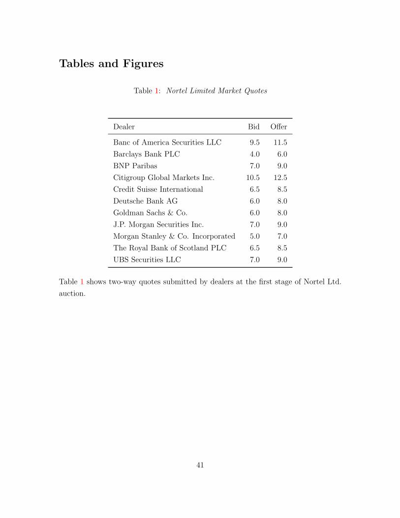
Tables and Figures

Table 1: Nortel Limited Market Quotes

Dealer Bid Offer

Banc of America Securities LLC 9.5 11.5

Barclays Bank PLC 4.0 6.0

BNP Paribas 7.0 9.0

Citigroup Global Markets Inc. 10.5 12.5

Credit Suisse International 6.5 8.5

Deutsche Bank AG 6.0 8.0

Goldman Sachs & Co. 6.0 8.0

J.P. Morgan Securities Inc. 7.0 9.0

Morgan Stanley & Co. Incorporated 5.0 7.0

The Royal Bank of Scotland PLC 6.5 8.5

UBS Securities LLC 7.0 9.0

Table 1 shows two-way quotes submitted by dealers at the first stage of Nortel Ltd.

auction.

41

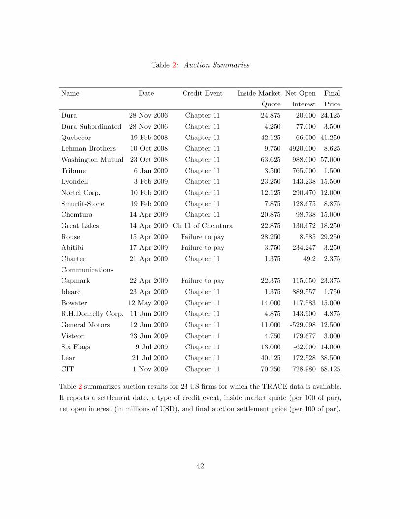
Table 2: Auction Summaries

Name Date Credit Event Inside Market Net Open Final

Quote Interest Price

Dura 28 Nov 2006 Chapter 11 24.875 20.000 24.125

Dura Subordinated 28 Nov 2006 Chapter 11 4.250 77.000 3.500

Quebecor 19 Feb 2008 Chapter 11 42.125 66.000 41.250

Lehman Brothers 10 Oct 2008 Chapter 11 9.750 4920.000 8.625

Washington Mutual 23 Oct 2008 Chapter 11 63.625 988.000 57.000

Tribune 6 Jan 2009 Chapter 11 3.500 765.000 1.500

Lyondell 3 Feb 2009 Chapter 11 23.250 143.238 15.500

Nortel Corp. 10 Feb 2009 Chapter 11 12.125 290.470 12.000

Smurfit-Stone 19 Feb 2009 Chapter 11 7.875 128.675 8.875

Chemtura 14 Apr 2009 Chapter 11 20.875 98.738 15.000

Great Lakes 14 Apr 2009 Ch 11 of Chemtura 22.875 130.672 18.250

Rouse 15 Apr 2009 Failure to pay 28.250 8.585 29.250

Abitibi 17 Apr 2009 Failure to pay 3.750 234.247 3.250

Charter 21 Apr 2009 Chapter 11 1.375 49.2 2.375

Communications

Capmark 22 Apr 2009 Failure to pay 22.375 115.050 23.375

Idearc 23 Apr 2009 Chapter 11 1.375 889.557 1.750

Bowater 12 May 2009 Chapter 11 14.000 117.583 15.000

R.H.Donnelly Corp. 11 Jun 2009 Chapter 11 4.875 143.900 4.875

General Motors 12 Jun 2009 Chapter 11 11.000 -529.098 12.500

Visteon 23 Jun 2009 Chapter 11 4.750 179.677 3.000

Six Flags 9 Jul 2009 Chapter 11 13.000 -62.000 14.000

Lear 21 Jul 2009 Chapter 11 40.125 172.528 38.500

CIT 1 Nov 2009 Chapter 11 70.250 728.980 68.125

Table 2 summarizes auction results for 23 US firms for which the TRACE data is available.

It reports a settlement date, a type of credit event, inside market quote (per 100 of par),

net open interest (in millions of USD), and final auction settlement price (per 100 of par).

42

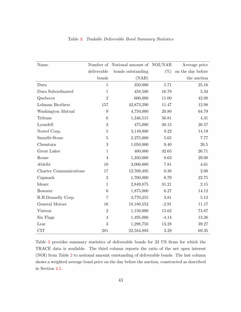
Table 3: Tradable Deliverable Bond Summary Statistics

Name Number of Notional amount of NOI/NAB Average price

deliverable bonds outstanding (%) on the day before

bonds (NAB) the auction

Dura 1 350,000 5.71 25.16

Dura Subordinated 1 458,500 16.79 5.34

Quebecor 2 600,000 11.00 42.00

Lehman Brothers 157 42,873,290 11.47 12.98

Washington Mutual 9 4,750,000 20.80 64.79

Tribune 6 1,346,515 56.81 4.31

Lyondell 3 475,000 30.15 26.57

Nortel Corp. 5 3,149,800 9.22 14.19

Smurfit-Stone 5 2,275,000 5.65 7.77

Chemtura 3 1,050,000 9.40 26.5

Great Lakes 1 400,000 32.65 26.71

Rouse 4 1,350,000 0.63 29.00

Abitibi 10 3,000,000 7.81 4.61

Charter Communications 17 12,769,495 0.38 2.00

Capmark 2 1,700,000 6.79 22.75

Idearc 1 2,849,875 31.21 2.15

Bowater 6 1,875,000 6.27 14.12

R.H.Donnelly Corp. 7 3,770,255 3.81 5.12

General Motors 16 18,180,552 -2.91 11.17

Visteon 2 1,150,000 15.62 74.87

Six Flags 4 1,495,000 -4.14 13.26

Lear 3 1,298,750 13.28 39.27

CIT 281 22,584,893 3.29 69.35

Table 3 provides summary statistics of deliverable bonds for 23 US firms for which the

TRACE data is available. The third column reports the ratio of the net open interest

(NOI) from Table 2 to notional amount outstanding of deliverable bonds. The last column

shows a weighted average bond price on the day before the auction, constructed as described

in Section 4.1.

43

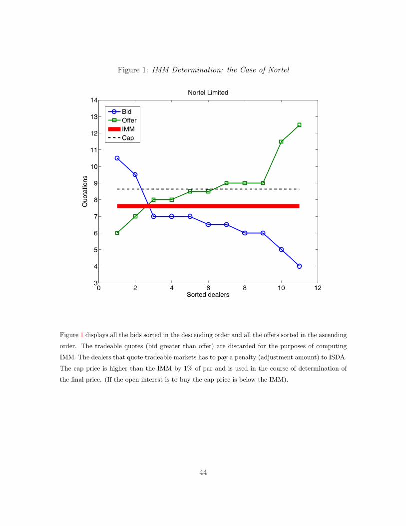
Figure 1: IMM Determination: the Case of Nortel

0 2 4 6 8 10 123

4

5

6

7

8

9

10

11

12

13

14

Sorted dealers

Quo

tatio

nsNortel Limited

BidOfferIMMCap

Figure 1 displays all the bids sorted in the descending order and all the offers sorted in the ascending

order. The tradeable quotes (bid greater than offer) are discarded for the purposes of computing

IMM. The dealers that quote tradeable markets has to pay a penalty (adjustment amount) to ISDA.

The cap price is higher than the IMM by 1% of par and is used in the course of determination of

the final price. (If the open interest is to buy the cap price is below the IMM).

44

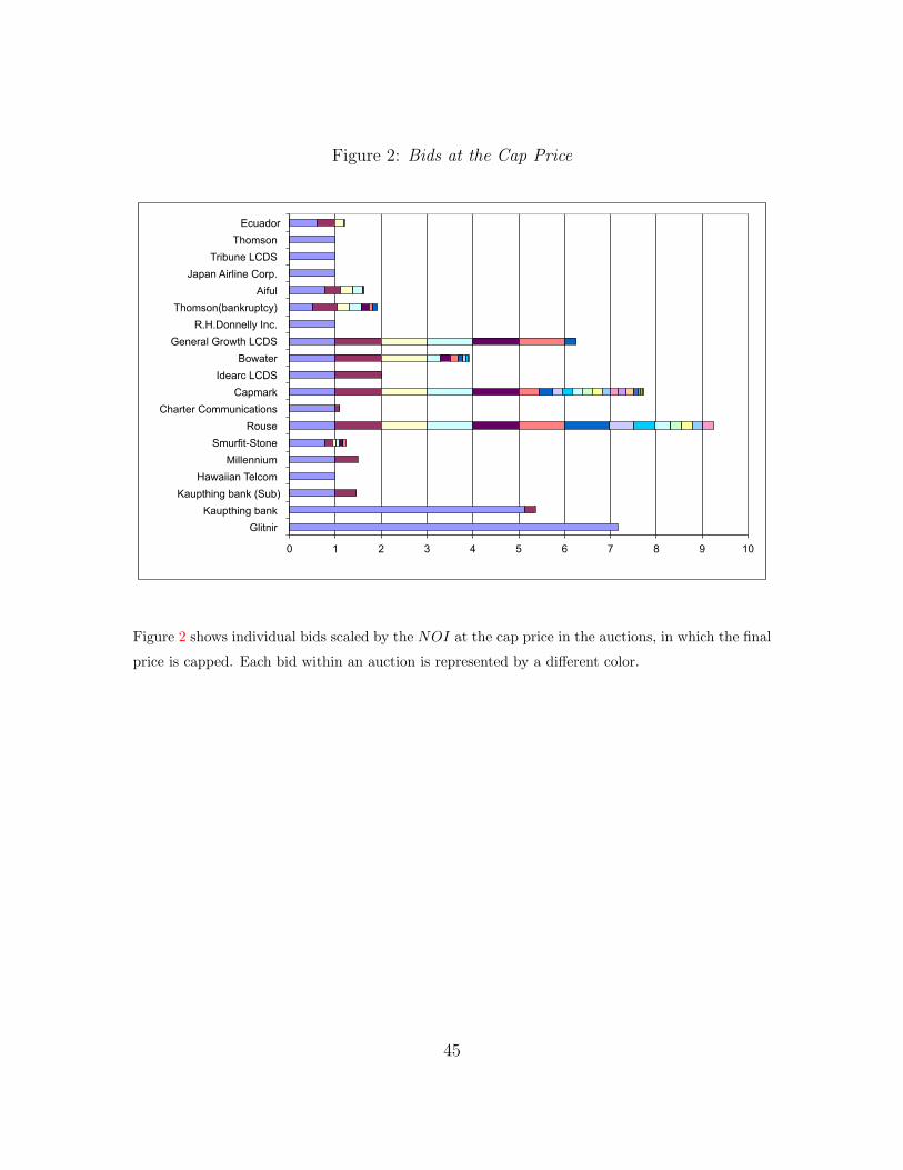
Figure 2: Bids at the Cap Price

0 1 2 3 4 5 6 7 8 9 10

Glitnir Kaupthing bank

Kaupthing bank (Sub) Hawaiian Telcom

Millennium Smurfit-Stone

Rouse Charter Communications

Capmark Idearc LCDS

Bowater General Growth LCDS

R.H.Donnelly Inc. Thomson(bankruptcy)

Aiful Japan Airline Corp.

Tribune LCDS Thomson

Ecuador

Figure 2 shows individual bids scaled by the NOI at the cap price in the auctions, in which the final

price is capped. Each bid within an auction is represented by a different color.

45

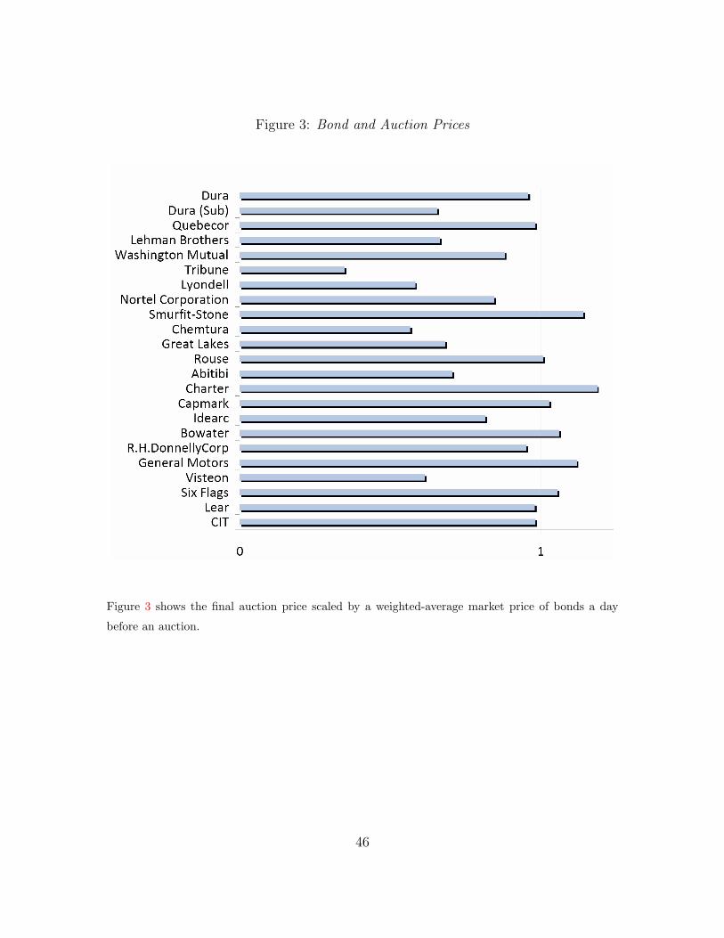
Figure 3: Bond and Auction Prices

Figure 3 shows the final auction price scaled by a weighted-average market price of bonds a day

before an auction.

46

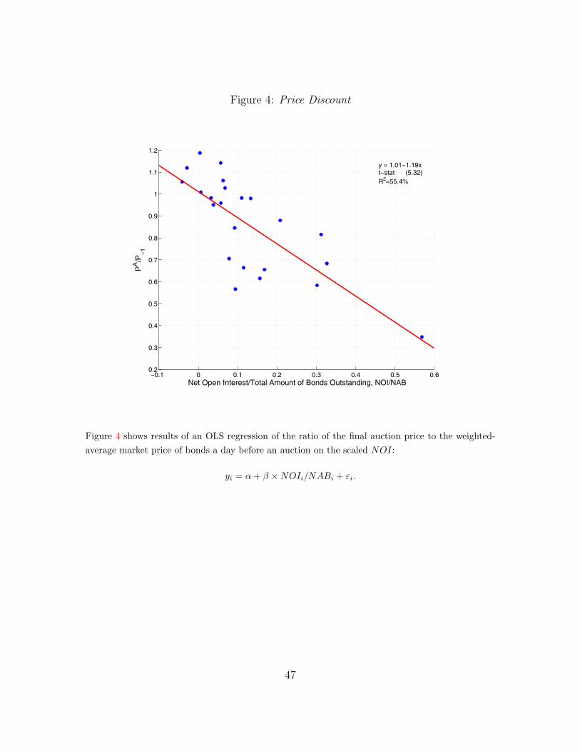
Figure 4: Price Discount

−0.1 0 0.1 0.2 0.3 0.4 0.5 0.60.2

0.3

0.4

0.5

0.6

0.7

0.8

0.9

1

1.1

1.2

Net Open Interest/Total Amount of Bonds Outstanding, NOI/NAB

PA/P

−1

y = 1.01−1.19xt−stat (5.32)R2=55.4%

Figure 4 shows results of an OLS regression of the ratio of the final auction price to the weighted-average market price of bonds a day before an auction on the scaled NOI:

yi = α+ β ×NOIi/NABi + εi.

47

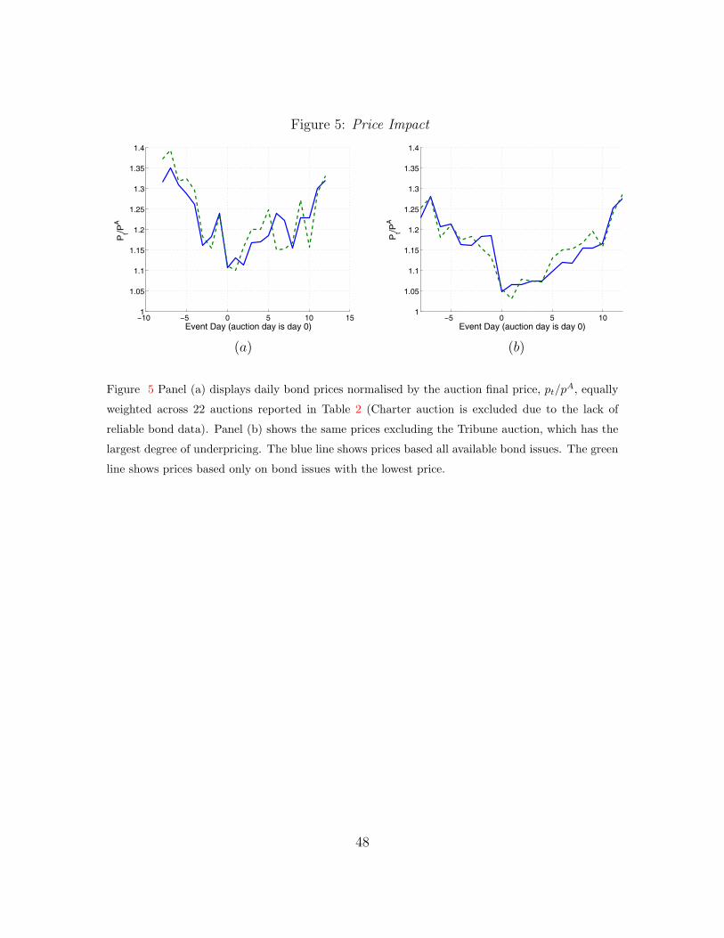
Figure 5: Price Impact

−10 −5 0 5 10 151

1.05

1.1

1.15

1.2

1.25

1.3

1.35

1.4

Event Day (auction day is day 0)

Pt/P

A

−5 0 5 101

1.05

1.1

1.15

1.2

1.25

1.3

1.35

1.4

Event Day (auction day is day 0)

Pt/P

A

(a) (b)

Figure 5 Panel (a) displays daily bond prices normalised by the auction final price, pt/pA, equally

weighted across 22 auctions reported in Table 2 (Charter auction is excluded due to the lack of

reliable bond data). Panel (b) shows the same prices excluding the Tribune auction, which has the

largest degree of underpricing. The blue line shows prices based all available bond issues. The green

line shows prices based only on bond issues with the lowest price.

48

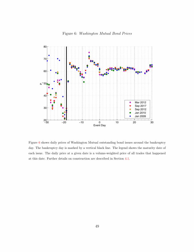
Figure 6: Washington Mutual Bond Prices

−30 −20 −10 0 10 20 3020

30

40

50

60

70

80

Event Day

Pt

Mar 2012 Sep 2017Sep 2012Jan 2010Jan 2009

Figure 6 shows daily prices of Washington Mutual outstanding bond issues around the bankruptcy

day. The bankruptcy day is marked by a vertical black line. The legend shows the maturity date of

each issue. The daily price at a given date is a volume-weighted price of all trades that happened

at this date. Further details on construction are described in Section 4.1.

49