CDS INDEX OPTIONS UNDER INCOMPLETE … · Alexander Herbertsson and Rüdiger Frey December 2016 ISSN 1403-2473 (print) ... Schmidt (2012) solve this problem using the innovations

Department of Economics

School of Business, Economics and Law at University of Gothenburg

Vasagatan 1, PO Box 640, SE 405 30 Göteborg, Sweden

+46 31 786 0000, +46 31 786 1326 (fax)

www.handels.gu.se [email protected]

WORKING PAPERS IN ECONOMICS

No 685

CDS INDEX OPTIONS UNDER INCOMPLETE

INFORMATION

Alexander Herbertsson and Rüdiger Frey

December 2016

ISSN 1403-2473 (print) ISSN 1403-2465 (online)

CDS INDEX OPTIONS UNDER INCOMPLETE INFORMATION

ALEXANDER HERBERTSSON AND RUDIGER FREY

Abstract. We derive practical formulas for CDS index spreads in a credit risk model underincomplete information. The factor process driving the default intensities is not directlyobservable, and the filtering model of Frey & Schmidt (2012) is used as our setup. In thisframework we find a computationally tractable expressions for the payoff of a CDS indexoption which naturally includes the so-called armageddon correction. A lower bound forthe price of the CDS index option is derived and we provide explicit conditions on thestrike spread for which this inequality becomes an equality. The bound is computationallyfeasible and do not depend the noise parameters in the filtering model. We outline how toexplicitly compute the quantities involved in the lower bound for the price of the credit indexoption as well as implement and calibrate this model to market data. A numerical study isperformed where we show that the lower bound in our model can be several hundred percentbigger compared with models which assume that the CDS index spreads follows a log-normalprocess. Also a systematic study is performed in order to understand the impact of variousmodel parameters on CDS index options (and on the index itself).

Keywords: Credit risk; CDS index; CDS index options; intensity-based models; depen-dence modelling; incomplete information; nonlinear filtering; numerical methods

JEL Classification: G33; G13; C02; C63; G32.

1. Introduction

The development of liquid markets for synthetic credit index products such as CDS indexswaps has led to the creation of derivatives on these products, most notably credit indexoptions, sometimes also denoted CDS index options. Essentially the owner of such an optionhas the right to enter at the maturity date of the option into a protection buyer position ina swap on the underlying CDS index at a prespecified spread; moreover, upon exercise heobtains the cumulative loss of the index portfolio up to the maturity of the option. Creditindex options have gained a lot interest the last turbulent years since they allow investors tohedge themselves against broad movements of CDS index spreads or to trade credit volatility.

To date the pricing and the hedging of these options is largely an unresolved problem.In practice this contract is priced by a fairly ad hoc approach: it is assumed that the loss-adjusted spread of the CDS index at the maturity of the option is lognormally distributedunder a martingale measure corresponding to a suitable numeraire, and the price of theoption is then computed via the Black formula. Details are described for instance in Morini& Brigo (2011) or Rutkowski & Armstrong (2009). However, beyond convenience there isno justification for the lognormality assumption in the literature. In particular, it is unclearif a dynamic model for the evolution of spreads and credit losses can be constructed thatsupports the lognormality assumption and the use of the Black formula, and there is noempirical justification for this assumption either.

The research of Alexander Herbertsson was supported by AMAMEF travel grants 2206 and 2678, by theJan Wallanders and Tom Hedelius Foundation and by Vinnova.

The research of Rudiger Frey was supported by Deutsche Forschungsgemeinschaft.1

2 ALEXANDER HERBERTSSON AND RUDIGER FREY

In this paper we therefore propose a different route for pricing and hedging credit indexoptions, which is based on a full dynamic credit risk model. We use a new, information-based approach to credit risk modelling proposed in Frey & Schmidt (2012) where prices oftraded credit derivatives are given by the solution of a nonlinear filtering problem. Frey &Schmidt (2012) solve this problem using the innovations approach to nonlinear filtering andderive in particular the Kushner-Stratonovich SDE describing the dynamics of the filteringprobabilities. Moreover, they give interesting theoretical results on the dynamics of the creditspreads and on risk minimizing hedging strategies.

Our paper use the filtering model of Frey & Schmidt (2012) in order to derive computa-tionally practical formulas for a CDS index under the market filtration. The market filtrationrepresents incomplete information since the background factor process driving the defaultintensities is observed with noise. Furthermore, in this model we derive computationallytractable formula for the payoff of a CDS index option. The formula naturally includes theso-called armageddon correction and is obtained without introducing a change of pricingmeasure, which is the case in the previous literature, see e.g. in Morini & Brigo (2011) orRutkowski & Armstrong (2009). We also derive a lower bound for price of the CDS indexoption and provide explicit conditions on the strike spread for which this inequality becomesan equality. The lower bound is computationally tractable and do not depend on any ofthe noise parameters in the filtering model. We then outline how to explicitly compute thequantities involved in the lower bound for the price of the credit index option. Furthermore, asystematic study is performed in order to understand the impact of various model parameterson these index options (and on the index itself).

Options on a CDS index have been studied in for example Pedersen (2003), Jackson (2005),Liu & Jackel (2005), Doctor & Goulden (2007), Rutkowski & Armstrong (2009), Morini &Brigo (2011), Flesaker, Nayakkankuppam & Shkurko (2011) and Martin (2012). In all ofthese papers it is assumed that either the CDS index spread or the so called loss-adjustedCDS index spread at the maturity of the option is lognormally distributed under a martingalemeasure corresponding to a suitable numeraire, and the price of the option is then computedvia the Black formula. For a nice and compact overview of some of the above mentionedpapers, see pp.577-579 in Morini & Brigo (2011).

The idea of using filtering techniques in credit risk modelling to price credit derivatives anddefaultable bonds is not new. For example, Capponi & Cvitanic (2009) develops a structuralcredit risk framework which models the deliberate misreporting by insiders in the firm. Inthis setting the authors derive formulas for bond and stock prices which lead to a non-linearfiltering model. The model is calibrated with Kalman filtering and maximum likelihoodmethods. The authors then apply their setup to the Parmalat-case and the parameters arecalibrated against real data.

The paper Fontana & Runggaldier (2010) considers an intensity based credit risk modelwhere default intensities and interest rates are driven by a partly unobservable factor process.In this setup they state formulas for contingent claims given the filtration generated by theunobservable factor process and the default times. The authors then derive a nonlinear filtersystem describing the dynamics of the filtering distribution which is needed for pricing thederivatives in their framework. The parameters in the model are obtained via an expectedmaximum (EM) algorithm which includes solving the nonlinear filter system by using theextended Kalman filter and a linearization of the framework. The model and estimationmethod is applied on simulated data with successful results.

CDS INDEX OPTIONS UNDER INCOMPLETE INFORMATION 3

In Frey & Runggaldier (2010) the authors develops a mathematical framework for handlingfiltering problems in reduced-form credit risk models.

The rest of the paper is organized as follows. First, in Section 2 we give a brief introductionto how a CDS index works and then present a model independent expression for the so calledCDS index spread. Section 2 also introduces options on the CDS index and provides a formulafor the payoff such an option which holds for any framework modelling the dynamics of thedefault times in the underlying credit portfolio. Then, in Section 3 we briefly describe themodel used in this paper, originally presented in Frey & Schmidt (2012). Section 4 givesa short recapitulation of the the Kushner-Stratonovich SDE describing the dynamics of thefiltering probabilities in the models, where we in particular focus on a homogeneous portfolio.Next, Section 5 describes the main building blocks that will be necessary to find formulasfor portfolio credit derivatives such as e.g. the CDS index as well as credit index options.Examples of such building blocks are the conditional survival distribution, the conditionalnumber of defaults and the conditional loss distribution. In Section 6 we use the results fromSection 5 to derive computational tractable formulas for the CDS index in the model presentedin Section 3. This will be done in a homogeneous portfolio. Continuing, in Section 7 we derivea practical formula for the payoff of a CDS index option in the nonlinear filtering modell. Thisformula will be used with Monte Carlo simulations in order to find approximations to the priceof options on a CDS index in the filtering framework. Further, a lower bound for the priceof the CDS index option is derived and we provide explicit conditions on the strike spreadfor which this inequality becomes an equality. The bound is computationally feasible and donot depend the noise parameters in the filtering model. We then outline how to explicitlycompute the quantities involved in the lower bound for the price of the credit index option.

Finally, in Section 8 we discuss how to estimate or calibrate the parameters in the filteringmodel introduced in Section 3 and also calibrate our model and present different numericalresults for prices of options on a CDS index.

2. The CDS index and credit index options

In this section we will discuss the CDS index and options on this index. First, Subsection2.1 gives a brief introduction to how a CDS index works. Then, in Subsection 2.2 we outlinemodel independent expression for the CDS index spread. Finally, Subsection 2.3 introducesoptions on the CDS index, sometimes denoted by credit index options, and uses the resultform Subsection 2.2 to provide a formula for the payoff such an option which holds for anyframework modelling the dynamics of the default times in the underlying credit portfolio.

2.1. Structure of a CDS index. Consider a portfolio consisting of m equally weightedobligors. An index Credit Default Swap (often denoted CDS index or index CDS ) for aportfolio of m obligors, entered at time t with maturity T , is a financial contract betweena protection buyer A and protection seller B with the following structure. The CDS indexgives A protection against all credit losses among the m obligors in the portfolio up to timeT where t < T . Typically, T = t+ T for T = 3, 5, 7, 10 years. More specific, at each defaultin the portfolio during the period [t, T ], B pays A the credit suffered loss due to the default.Thus, the accumulated value payed by B to A in the period [t, T ] is the total credit loss in theportfolio during the period from t to time T . As a compensation for this A pays B a fixed feeS(t, T ) multiplied what is left in the portfolio at each payment time which are done quarterlyin the period [t, T ]. The fee S(t, T ) is set so expected discounted cash-flows between A andB is equal at time t and S(t, T ) is called the CDS index spread with maturity T − t. For


t = 0 (i.e. ”today”) so that T = T we sometimes denote S(0, T ) by S(T ) and the quantityS(T ) can be observed on a daily basis for standard CDS indexes such as iTraxx Europe andthe CDX.NA.IG index, for maturities T = 3, 5, 7, 10 years. The quarterly payments fromB to A are done on the IMM dates 20th of March, 20th of June, 20th of September and20th of December. Standardized indices such as iTraxx are updated twice a year on so called”index-rolls” which takes place on the two IMM dates 20th of March and 20th of September.The most recent rolled CDS index is referred to the ”on-the-run-index”. Indices rolled onprevious dates are refereed to as ”off-the-run-indices”. A T -year on-the-run index issued on20th of March a given year will mature on 20th of June T years later. Similarly, a T -yearon-the-run index issued on 20th of September a given year will mature on 20th of DecemberT years later. Thus, the effective protection period will be somewhere between T − 0.25 andT − 0.25 years. For example, a 5-year on-the-run CDS index entered on 20th of March willhave a maturity of 5.25 years but if it is entered on the 16th of September the same year itwill have a maturity of around 4.75 years. As we will see later, these maturity details willplay an important role when pricing options on CDS indices. For more on practical detailsregarding the CDS index, see e.g Markit (2016) or O’Kane (2008).

In order to give a more explicit description of the CDS index spread S(t, T ) we need tointroduce some further notations and concepts which is done in the next subsection.

2.2. The CDS index spread. In this subsection we give a quantitative description of theCDS index spread. First we need to introduce some notation. Let (Ω,G,Q) be the underlyingprobability space assumed in the rest of this paper. We set Q to be a risk neutral probabilitymeasure which exist (under rather mild condition) if arbitrage possibilities are ruled out.Furthermore, let F = (Ft)t≥0 be a filtration representing the full market information ateach time point t. Consider a portfolio consisting of m equally weighted obligors with defaulttimes τ1, τ2 . . . , τm adapted to the filtration (Ft)t≥0 and let ℓ1, ℓ2, . . . , ℓm be the correspondingindividual credit losses at each default time. Typically ℓi = (1−φi)/m where φi is a constantrepresenting the recovery rate for obligor i. The credit loss for this portfolio at time t is thendefined as

∑mi=1 ℓi1τi≤t. Similarly, the number of defaults in the portfolio up to time t,

denoted by Nt, is Nt =∑m

i=1 1τi≤t. Note that if the individual loss is constant and identicalfor all obligors so that ℓ = ℓ1 = ℓ2 = . . . = ℓm then the normalized credit loss Lt is given byLt =

ℓmNt. In the rest of this paper we will assume that the individual loss is constant and

identical for all obligors where 1− φ = ℓ = ℓ1 = ℓ2 = . . . = ℓm and we therefore have that

Lt =1− φ

mNt where Nt =

m∑

i=1

1τi≤t. (2.2.1)

Finally, for t < u we let B(t, u) denote the discount factor between t and u, that isB(t, u) = Bt

Bu

where Bt is the risk free savings account. Unless explicitly stated, we will assume that therisk free interest rate is constant and given by r so that Bt = ert and B(t, u) = e−r(u−t).

Let T > t and consider an CDS index entered at time t with maturity T on the portfoliowith loss process Lt. In view of the above notation we can now define the (stochastic)discounted payments VD(t, T ) from A to B during the period [t, T ], and VP (t, T ) from B toA in the timespan [t, T ], as follows

VD(t, T ) =

∫ T

t

B(t, s)dLs and VP (t, T ) =1

4

⌈4T ⌉∑

n=nt

B(t, tn)

(1− Ntn

m

)(2.2.2)


where nt denotes nt = ⌈4t⌉ + 1 and tn = n4 . We here emphasize that we have dropped the

accrued term in VP (t, T ) and also ignored the accrued premium up to the first payment datein VP (t, T ). The expected value of the default and premium legs, conditional on the marketinformation Ft are given by

DL(t, T ) = E [VD(t, T ) | Ft] and PV (t, T ) = E [VP (t, T ) | Ft] (2.2.3)

that is

DL(t, T ) = E

[∫ T

t

B(t, s)dLs

∣∣∣∣Ft

](2.2.4)

and

PV (t, T ) =1

4

⌈4T ⌉∑

n=nt

B(t, tn)

(1− 1

mE [Ntn | Ft]

). (2.2.5)

In view of structure of a CDS index described in Subsection 2.1, the CDS index spread S(t, T )at time t with maturity T is defined as

S(t, T ) =DL(t, T )

PV (t, T )(2.2.6)

or more explicit, using (2.2.4) and (2.2.5)

S(t, T ) =E[∫ T

tB(t, s)dLs

∣∣∣Ft

]

14

∑⌈4T ⌉n=nt

B(t, tn)(1− 1

mE [Ntn | Ft]

) . (2.2.7)

The definition of S(t, T ) in (2.2.6) is done assuming that not all obligors have defaulted inthe portfolio at time t, that is S(t, T ) is defined on the event Nt < m. In the event of aso-called armageddon scenario at time t where Nt = m (i.e. all obligors in the portfolio havedefaulted up to time t), we see that the premium leg VP (t, T ) in (2.2.2) is zero at time t,which obviously makes the definition of the spread S(t, T ) invalid. Note that for t = 0 (i.e.today) the quantity S(0, T ) can be observed on a daily basis for standard CDS indexes suchas iTraxx Europe and the CDX.NA.IG index, for maturities T = 3, 5, 7, 10 years.

We here remark that the outline for the CDS index spread presented in this subsectionholds for any framework modelling the dynamics of the default times in the underlying creditportfolio. Consequently, the filtration Ft used in this subsection can be generated by anycredit portfolio model.

2.3. The CDS index option. In this subsection we introduce options on the CDS indexand discuss how they work. Then we use the result form Subsection 2.2 in order to providea formula for the payoff of such an option, which holds for any framework modelling thedynamics of the default times in the underlying credit portfolio. First, let us give the definitionof a payer CDS index option, which is the same as Definition 2.3 in Morini & Brigo (2011)and Definition 2.4 in Rutkowski & Armstrong (2009).

Definition 2.1. A payer CDS index option (sometimes called a put CDS index option)with strike κ and exercise date t written on a CDS index with maturity T is a financialderivative which gives the protection buyer A the right but not the obligation to enter theCDS index with the protection seller B at time t with a fixed spread κ and protection periodT − t. Moreover, at the exercise date t, the protection seller B also pays A the accumulatedcredit loss occurred during the period from the inception time of the option (at time 0, i.e.


”today”) to the exercise date t, that is B pays A the loss Lt at time t, which is referred to asthe front end protection.

The payoff Π(t, T ;κ) at the exercise time t for a payer CDS index option seen from theprotection buyer A’s point of view, is given by

Π(t, T ;κ) =(PV (t, T ) (S(t, T )− κ) 1Nt<m + Lt

)+(2.3.1)

where PV (t, T ) is defined as in (2.2.5). For an analogues expression of (2.3.1), see e.g.Equation (2.18) on p.1045 in Rutkowski & Armstrong (2009) or Equation (2.3) on p.577in Morini & Brigo (2011). Note that the CDS index at time t is entered only if there areany nondefaulted obligors left in the portfolio at time t, which explains the presence of theindicator function of the event Nt < m in the expression for the payoff Π(t, T ;κ) in (2.3.1).However, the front end protection Lt will be paid out by A at time t even if the eventNt = m occurs. From (2.2.6) we have that

PV (t, T ) (S(t, T )− κ) 1Nt<m = DL(t, T )1Nt<m − κPV (t, T )1Nt<m. (2.3.2)

However, since Nt is a non-decreasing process where Nt ≤ m almost surely for all t ≥ 0 wehave from the definitions in (2.2.4) and (2.2.5) that

DL(t, T )1Nt=m = E

[∫ T

t

B(t, s)dLs

∣∣∣∣Ft

]1Nt=m = 0 and PV (t, T )1Nt=m = 0

(2.3.3)so we can use (2.3.3) to simplify (2.3.2) according to

PV (t, T ) (S(t, T )− κ) 1Nt<m = DL(t, T )− κPV (t, T ). (2.3.4)

We here remark that the observations (2.3.3) and (2.3.4) has also been done in Rutkowski &Armstrong (2009) and Morini & Brigo (2011), see e.g Equation (2.6) on p. 1040 in Rutkowski& Armstrong (2009) and Proposition 3.7 on p. 582 in Morini & Brigo (2011). By using (2.3.4)we can rewrite the payoff Π(t, T ;κ) in (2.3.1) as

Π(t, T ;κ) = (DL(t, T )− κPV (t, T ) + Lt)+ . (2.3.5)

The model outline for payer CDS index option presented in this subsection holds for anyframework modelling the dynamics of the default times in the underlying credit portfolio.Consequently, the filtration Ft used in this subsection can be generated by any credit portfoliomodel.

Before ending this section we briefly discuss some properties of CDS index options that arenot shared with e.g. standard equity options. First, we note that (2.3.1) or (2.3.5) impliesthat

limκ→∞

Π(t, T ;κ)1Nt<m = 0. (2.3.6)

Secondly, since the individual loss 1 − φ is constant and identical for all obligors and since

Lt = (1−φ)Nt

m, we have Lt1Nt=m = (1 − φ)1Nt=m which in (2.3.5) together with (2.3.3)

implies that

Π(t, T ;κ)1Nt=m = Lt1Nt=m = (1− φ)1Nt=m for all κ (2.3.7)

and consequently

limκ→∞

Π(t, T ;κ)1Nt=m = Lt1Nt=m = (1− φ)1Nt=m. (2.3.8)


So combining (2.3.6) and (2.3.8) renders

limκ→∞

Π(t, T ;κ) = (1− φ)1Nt=m a.s. (2.3.9)

For s ≤ t, the price Cs(t, T ;κ) of a payer CDS index option at time s with strike κ andexercise date t written on a CDS index with maturity T , is due to standard risk neutralpricing theory given by

Cs(t, T ;κ) = e−r(t−s)E [Π(t, T ;κ) | Fs] . (2.3.10)

Furthermore, since

Π(t, T ;κ) = Π(t, T ;κ)1Nt<m +Π(t, T ;κ)1Nt=m = Π(t, T ;κ)1Nt<m + (1− φ)1Nt=m

then for s ≤ t, the price Cs(t, T ;κ) can be expressed as

Cs(t, T ;κ) = e−r(t−s)E[Π(t, T ;κ)1Nt<m

∣∣Fs

]+ (1− φ)e−r(t−s)Q [Nt = m | Fs] . (2.3.11)

From (2.3.6) and (2.3.8) together with the dominated convergence theorem, we conclude thatif s ≤ t then

limκ→∞

Cs(t, T ;κ) = (1− φ)e−r(t−s)Q [Nt = m | Fs] (2.3.12)

which is in line with the results in (2.3.9). Also note that the results in this section holds forany framework modelling the dynamics of the default times in the underlying credit portfolio.In this paper our numerical examples will be performed for s = 0 which in (2.3.12) impliesthat

limκ→∞

C0(t, T ;κ) = (1− φ)e−rtQ [Nt = m] (2.3.13)

Recall that in the standard Black-Scholes model the call option price converges to zero asthe strike price converges to infinity but due to the front end protection this will not hold forpayer CDS index option, as is clearly seen in Equation (2.3.11), (2.3.12) and (2.3.13).

2.4. Some previous models for the CDS index option. In this subsection we will discusssome previously studied models and one of these models will be used as a benchmark to theframework developed in this paper.

Options on a CDS index have been studied in for example Pedersen (2003), Jackson (2005),Liu & Jackel (2005), Doctor & Goulden (2007), Rutkowski & Armstrong (2009), Morini &Brigo (2011), Flesaker et al. (2011) and Martin (2012). In all of these papers it is assumedthat either the CDS index spread or the so called loss-adjusted CDS index spread at thematurity of the option is lognormally distributed under a martingale measure correspondingto a suitable numeraire, and the price of the option is then computed via the Black formula.For a nice and compact overview of some of the above mentioned papers, see pp.577-579 inMorini & Brigo (2011).

We will here give a very brief review of the results in some of these papers since thesewill introduce formulas that we will use as a comparison when benchmarking with our modelpresented in Section 7.

As discussed in Morini & Brigo (2011), in the initial market approach for pricing CDSindex options, the price CIM

s (t, T ;κ) at time s ≤ t of a payer CDS index option with strikeκ and exercise date t written on a CDS index with maturity T , is modelled as (see also e.g.Equation (2.4) in Morini & Brigo (2011)))

CIMs (t, T ;κ) = e−r(t−s)E [VP (t, T ) | Fs]C

B (S(s, T ), κ, t, σ) + e−r(t−s)E [Lt | Fs] (2.4.1)


where we have used the same notation as in Subsection 2.3 and where C(B) (S,K, T, σ) is theBlack-formula, i.e.

CB (S,K, T, σ) = SN(d1)−KN(d2)

d1 =ln(S/K) + 1

2σ2T

σ√T

, d2 = d1 − σ√T

(2.4.2)

and N(x) is the distribution function for a standard normal random variable. As pointedout by Pedersen (2003), and also emphasized in Morini & Brigo (2011), the formula (2.4.1)does not incorporate the front end protection in a correct way given the payoff expression inEquation (2.3.1). To overcome the problem of a wrong inclusions of the front end protection inthe option formula, several papers proposed an improvement of the Black-framework, see forexample Doctor & Goulden (2007). The idea is to introduce a so called loss-adjusted marketindex spread defined, see e.g. Equation (2.6) in Morini & Brigo (2011)). More specific, let tbe the exercise date for a CDS index option and for u < t < T let DLt(u, T ) and PVt(u, T )denote

DLt(u, T ) = E [B(u, t)VD(t, T ) | Fu] and PVt(u, T ) = E [B(u, t)VP (t, T ) | Fu] (2.4.3)

where VD(t, T ) and VP (t, T ) are given by (2.2.2). Next, define loss-adjusted market index

spread St(u, T ) for u ≤ t ≤ T as

St(u, T ) =DLt(u, T ) + E [B(u, t)Lt | Fu]

PVt(u, T ). (2.4.4)

Note that if u = t then B(t, t) = 1, PVt(t, T ) = PV (t, T ) and Lt is Ft-measurable which

reduces St(t, T ) in (2.4.4) to

St(t, T ) = S(t, T ) +Lt

PV (t, T )(2.4.5)

where S(t, T ) is defined as in (2.2.6). Also, if t = 0 then L0 = 0 so (2.4.5) then gives

S0(0, T ) = S(0, T ) (2.4.6)

which makes perfect sense. The benefit with using the loss-adjusted market index spreadSt(u, T ) in (2.4.4) is that payoff Π(t, T ;κ) at the exercise time t > 0 for a payer CDS indexoption as given in (2.3.5) can via (2.4.5) be rewritten as

Π(t, T ;κ) = PV (t, T )(St(t, T )− κ

)+. (2.4.7)

Hence, by using PVt(u, T ) as a numeraire for u ≤ t ≤ T and assuming that St(u, T ) islognormally distributed under a martingale measure corresponding to the chosen numeraire,one can at time s ≤ t price a payer CDS index option with exercise time t via (2.4.7) and theBlack formula according to

Cs(t, T ;κ) = e−r(t−s)E [VP (t, T ) | Fs]CB(St(s, T ), κ, t, σ

)(2.4.8)

where we assumed a constant interest rate r. Furthermore, σ is the constant volatility of theloss-adjusted market index spread St(u, T ) and the quantity C(B) (S,K, T, σ) is the same asin (2.4.2), see also e.g. Equation (2.8) on p.578 in Morini & Brigo (2011).


Remark 2.2. As pointed out on pp.578-579 in Morini & Brigo (2011), there are three mainproblems with the formula (2.4.8) and the definition of the loss-adjusted market index spread

in (2.4.4). The first problem is that loss-adjusted market index spread St(u, T ) in (2.4.4)is not defined when PVt(u, T ) = 0, i.e. when Nu = m. The second problem is that whenPVt(u, T ) = 0, the formula (2.4.8) is undefined and will not be consistent with the expressionin (2.3.12) which must holds for any framework modelling the dynamics of the default timesin the underlying credit portfolio for the CDS index. The third problem with (2.4.4) is thatsince PVt(u, T ) = 0 on Nu = m and if Q [Nu = m] > 0 (which is true for most standardportfolio credit models when u > 0), then PVt(u, T ) will not be strictly positive a.s. and willtherefore as a numeraire not lead to a pricing measure that is equivalent with the risk-neutralpricing measure Q.

Rutkowski & Armstrong (2009) and Morini & Brigo (2011) have independently developedan approach which overcomes the three problems stated in Remark 2.2 connected to the theloss-adjusted market index spread in (2.4.4) and the pricing formula (2.4.8). The main ideas inRutkowski & Armstrong (2009) and Morini & Brigo (2011) work as follows (following mainly

the notation of Morini & Brigo (2011)). Let τ (1) ≤ τ (2) ≤ . . . ≤ τ (m) be the ordering of thedefault times τ1, τ2 . . . , τm in the underlying credit portfolio that creates the CDS index. Forexample, τ (m) is the maximum of τi, that is

τ := τ (m) = max (τ1, τ2 . . . , τm) (2.4.9)

where we for notational convenience denote τ (m) by τ . So with Nt defined as in previoussections, i.e. Nt =

∑mi=1 1τi≤t we immediately see that

τ > t = Nt < m and τ ≤ t = Nt = m . (2.4.10)

Next, both Rutkowski & Armstrong (2009) and Morini & Brigo (2011) assumes the exis-

tence of an auxiliary filtration Ht such that underlying full market information Ft can bedecomposed as

Ft = Jt ∨ Ht (2.4.11)

Jt = σ (τ ≤ s; s ≤ t) (2.4.12)

where τ is not a Ht-stopping time. Rutkowski & Armstrong (2009) and Morini & Brigo

(2011) remarks that one possible construction of (2.4.11)-(2.4.12) is to let Ht be given by

Ht = Gt ∨m−1k=1 J (k)

t (2.4.13)

where for each k the filtration J (k)t is defined as

J (k)t = σ

(τ (k) ≤ s; s ≤ t

)(2.4.14)

and Gt in (2.4.13) is a filtration excluding default information, i.e Gt is the ”default free”information. Typically Gt is a sigma-algebra generated by a d-dimensional stochastic process(Xt)t≥0 so GX

t = σ(Xs; s ≤ t) where Xt = (Xt,1,Xt,2, . . . ,Xt,d) do not contain the randomvariables τ1, τ2 . . . , τm in their dynamics. Such constructions are standard in conditionalindependent dynamic portfolio credit models, see e.g in Lando (2004) or McNeil, Frey &

Embrechts (2005). From the construction in (2.4.11)-(2.4.13) it is clear that τ is not a Ht-stopping time. In Remark 3.5 on p.580 in Morini & Brigo (2011) the authors point out that


the construction in (2.4.11)-(2.4.12) may under certain, not unreasonable model assumptions,

not be possible to construct. Now, for u < t < T let DLt(u, T ) and P V t(u, T ) denote

DLt(u, T ) = E[B(u, t)VD(t, T ) | Hu

]and P V t(u, T ) = E

[B(u, t)VP (t, T ) | Hu

]

(2.4.15)

where VD(t, T ) and VP (t, T ) are given by (2.2.2). Next, define St(u, T ) as (see Rutkowski &Armstrong (2009) or Morini & Brigo (2011))

St(u, T ) =DLt(u, T ) + E

[1τ>tB(u, t)Lt

∣∣ Hu

]

P V t(u, T )(2.4.16)

where t typically is the exercise date for a CDS index option. Furthermore, Morini & Brigo(2011) assumes that

Q[τ > s | Hs

]> 0 a.s. for any s > 0 (2.4.17)

and Rutkowski & Armstrong (2009) makes a similar assumption but on a bounded intervalfor s. The reason for the assumption (2.4.17) is that in the derivations of the formulas forthe CDS-index spreads presented in Morini & Brigo (2011) and Rutkowski & Armstrong

(2009) the quantity Q[τ > s | Hs

]will emerge in the denominator of several expressions.

More specific, the choice (2.4.11)-(2.4.12) together with (2.4.17) will for s ≤ t make the

quantity P V t(u, T ) = E[B(u, t)VP (t, T ) | Hu

]to be strictly positive a.s. (see e.g. p.581

in Morini & Brigo (2011)) and can thus be used as a numeraire, which was observed bothin Rutkowski & Armstrong (2009) and Morini & Brigo (2011) independently of each other.Furthermore, Morini & Brigo (2011) and Rutkowski & Armstrong (2009) also shows that

under the condition (2.4.17) the spread St(u, T ) in (2.4.16) is well defined which thus solvesthe first and third problem specified in Remark 2.2. By using assumption (2.4.17) together

with the assumption that S(u, T ) in (2.4.16) follows a lognormal distribution under a measure

defined via P V t(u, T ), Morini & Brigo (2011) and Rutkowski & Armstrong (2009) prove thatfor s ≤ t the price for a payer CDS index option at time s with exercise date t via (2.4.7) isgiven by

Cs(t, T ;κ) = 1τ>se−r(t−s)E [VP (t, T ) | Fs]C

B(St(s, T ), κ, t, σ

)

+1τ>s

Q[τ > s | Hs

]E[1s<τ≤te

r(t−s)(1− φ)∣∣∣ Hs

]+ 1τ≤s(1− φ)e−r(t−s) (2.4.18)

where σ is the volatility of St(u, T ) under a suitable measure (see e.g. Corollary 4.3 in

Rutkowski & Armstrong (2009)). The quantity C(B) (S,K, T, σ) in (2.4.18) is the same as in(2.4.2). We assumed a constant interest rate r while Morini & Brigo (2011) and Rutkowski &Armstrong (2009) allows for a stochastic discount factor in (2.4.18), see e.g. Equation (2.29)in Rutkowski & Armstrong (2009) and Equation (4.1) and (4.4) in Morini & Brigo (2011).We note that if s > 0, then the second term in (2.4.18) is nontrivial to compute in practice.

However, an important practical case is to compute Cs(t, T ;κ) when s = 0, i.e. C0(t, T ;κ)(the numerical examples in Morini & Brigo (2011) are only done for the case s = 0 whileRutkowski & Armstrong (2009) do not provide any numerical examples of their formulas).


So letting s = 0 in (2.4.18) implies that C0(t, T ;κ) is given by the following expression

C0(t, T ;κ) = e−rtE [VP (t, T )]CB(St(0, T ), κ, t, σ

)+ e−rt(1 − φ)Q [Nt = m] (2.4.19)

where we used that τ ≤ t = Nt = m. So we clearly see that formula (2.4.19) is consistentwith (2.3.13) which must holds for any framework modelling the dynamics of the default timesin the underlying credit portfolio for the CDS index. Hence, this solves the second problempointed out in Remark 2.2. Also note that St(0, T ) will via (2.4.16) simplify to

St(0, T ) =DLt(0, T ) + E

[1τ>tB(0, t)Lt

]

P V t(0, T )

=DLt(0, T ) + E

[1τ>tB(0, t)Lt

]

PVt(0, T )

=DLt(0, T ) + E [B(0, t)Lt]− E

[1τ≤tB(0, t)Lt

]

PVt(0, T )

=DLt(0, T ) + E [B(0, t)Lt]

PVt(0, T )−

E[1τ≤tB(0, t)Lt

]

PVt(0, T )

= St(0, T ) −(1− φ)E

[B(0, t)1Nt=m

]

PVt(0, T )

(2.4.20)

where the second equality follows from (2.4.3) and (2.4.15) with u = 0 and last equality is

due to the definition of St(u, T ) in (2.4.4) and the fact that 1τ≤tLt = (1− φ)1Nt=m. Alsonote that if t = 0 then 1N0=m = 0 a.s. which together with (2.4.5) gives

St(0, T ) = S0(0, T ) = S(0, T ) (2.4.21)

which makes perfect sense. Furthermore, if we assume that the interest rate is deterministicwe can rewrite (2.4.20) as

St(0, T ) = St(0, T ) −(1− φ)Q [Nt = m]

E [VP (t, T )](2.4.22)

where VP (t, T ) is defined in (2.2.2).There are several numerical issues to be considered in (2.4.19). First, as pointed out

on p.1051 in Rutkowski & Armstrong (2009), since the loss adjusted spread St(u, T ) is notdirectly observable on the market at any time point u ≥ 0, it is quite challenging to estimatethe volatility σ of St(u, T ) where σ is used in the Black-formula present in (2.4.19). Secondly,computing the quantity Q [Nt = m] for large m (for example, m = 125 both in the iTraxxEurope and CDX NAG index) is numerically nontrivial and requires special attention even insimple standard portfolio credit models such as the one-factor Gaussian copula model. Notethat Q [Nt = m] emerges both in the second term of (2.4.19) aswell as in St(0, T ) used in theBlack-formula present in (2.4.19), as seen in (2.4.20) or (2.4.22).

While Rutkowski & Armstrong (2009) do not provide any numerical examples, Morini& Brigo (2011) uses a one-factor Gaussian copula model but do not specify which numer-ical method they use to compute Q [Nt = m]. There exists many methods for computingQ [Nt = k], 0 ≤ k ≤ m, in conditional independent models such as copula models, see forexample in Gregory & Laurent (2003) and Gregory & Laurent (2005).


In order to numerically benchmark the CDS index model presented in Section 3-7 againstMorini & Brigo (2011), we will also implement the model in Morini & Brigo (2011) using aone-factor Gaussian copula model just as Morini & Brigo (2011) do. Our choice of numericalmethod when computing Q [Nt = m] in (2.4.19) and (2.4.22) will be based on the normal ap-proximation of the mixed binomial distribution, similar to the method in Frey, Popp & Weber(2008). To be more specific, for any integer 1 ≤ k ≤ m we use the following approximationfor Q [Nt ≤ k] in the one-factor Gaussian copula model

Q [Nt ≤ k] ≈∫ ∞

−∞N

(k + 0.5−mpt(z)√mpt(z)(1 − pt(z)

)1√2π

e−z2

2 dz for k ≤ m (2.4.23)

where pt(z) is given by

pt(z) = N

(N−1 (Q [τ ≤ t])−√

ρz√1− ρ

)(2.4.24)

and N(x) is the distribution function for a standard normal random variable, ρ is the cor-relation parameters and τ has the same distribution as the exchangeable default times τiin the underlying credit portfolio, see e.g. Corollary 2.5 in Frey et al. (2008). The term 0.5in (2.4.23) is a so-called ”half-correction” which seem to produce better approximations thatthe ordinary normal approximation of a binomial distribution. Next, since

Q [Nt = m] = Q [Nt ≤ m]−Q [Nt ≤ m− 1] (2.4.25)

we use (2.4.23) with k = m − 1 and k = m in the right hand side of (2.4.25) to retrievean approximation to the quantity Q [Nt = m] in (2.4.19) and (2.4.22). Next we need to findan expression for Q [τ ≤ t] used in (2.4.23) via (2.4.24). A standard assumption made inthe homogeneous portfolio credit risk one-factor Gaussian copula model is that the defaulttimes τi have constant default intensity λ, that is they are exponentially distributed withparameter λ, i.e. if τ has the same distribution as τi then

Q [τ ≤ t] = 1− e−λt (2.4.26)

where λ is given by

λ =SM(T )

1− φ(2.4.27)

and SM(T ) is the market quote for the T -year CDS-index spread today and φ is the recoveryrate. The relation (2.4.27) is the so-called credit triangle, frequently used among marketpractitioners assuming a ”flat” CDS term structure, i.e. assuming that the default intensitywill be constant for all time points after t.

A derivation of the relation (2.4.27) in the case with quarterly payments is given in Propo-sition B.1 in Appendix B, since the existing proofs of (2.4.27) found in the litterature are onlydone in the unrealistic case when the CDS index premium is paid continuously. In practicethe CDS premiums are done quarterly.

Furthermore, note that we have used the CDS index spread SM(T ) in (2.4.27) because thisspread will in a homogeneous credit portfolio be identical to the the individual CDS spreadfor an obligor in the reference portfolio, see e.g. Proposition Lemma 6.1 in Herbertsson, Jang& Schmidt (2011). This ends the specification of how we compute Q [Nt = m]. In Figure 1we plot Q [Nt = m] for t = 9 months and m = 125 as function of the correlation parameter ρwhere we used (2.4.23)-(2.4.27) to compute Q [Nt = m] with φ = 40% and SM(5) = 200 bps.As can be seen in Figure 1, the effect of ρ on Q [Nt = m] will only come in to play when ρ


is bigger than 95% and for smaller ρ, the armageddon probability Q [Nt = m] will in practicebe neglible, see also Figure 5.1 in Morini & Brigo (2011)

ρ

0.7 0.75 0.8 0.85 0.9 0.95 1

Q[N

0.75

=12

5]

0

0.005

0.01

0.015

0.02

0.025Armageddon probability Q[N

0.75=125] as function of ρ for S(5)=200 bp

Figure 1. The Armageddon probabilityQ [N0.75 = 125] as function of the correlationρ = where S(0, 5) = 200 and φ = 40% bp.

So what is left to compute in (2.4.19) is St(0, T ). This is done in the following proposition.

Proposition 2.3. Consider a CDS index with maturity T on a homogeneous credit portfolio

where the obligors have constant default intensity λ. Then, with notation as above

St(0, T ) = 4(1 − φ)e−rt(1− e−

(r+λ)4

)(

λλ+r

(e−(r+λ)t − e−(r+λ)T

)+ 1− e−λt −Q [Nt = m]

)

e−(r+λ)nt

4 − e−(r+λ)(⌈4T⌉+1)

4

(2.4.28)where nt = ⌈4t⌉+ 1.

Proof. From (2.4.22) we have

St(0, T ) = St(0, T ) −(1− φ)Q [Nt = m]

E [VP (t, T )](2.4.29)

so we need explicit expressions for the quantities E [VP (t, T )] and St(0, T ). First, to findE [VP (t, T )] we use the exchangeability of the default times τi all having the same distri-bution as in (2.4.26), which in the definition of VP (t, T ) given by (2.2.2) with properties for


geometric series and some computations yields

E [VP (t, T )] =ert(e−

(r+λ)nt

4 − e−(r+λ)(⌈4T⌉+1)

4

)

4(1− e−

(r+λ)4

) (2.4.30)

where nt denotes nt = ⌈4t⌉ + 1 as in (2.2.2). Next, we provide an explicit expression for

St(0, T ) given by (2.4.4) with u = 0 and constant interest rate r, that is

St(0, T ) =DLt(0, T ) + e−rtE [Lt]

PVt(0, T )

=DLt(0, T ) + e−rt(1− φ)Q [τ ≤ t]

PVt(0, T )

=E [VD(t, T )]

E [VP (t, T )]+

(1− φ)Q [τ ≤ t]

E [VP (t, T )]

=ertE

[∫ T

te−rsdLs

]

E [VP (t, T )]+

(1− φ)Q [τ ≤ t]

E [VP (t, T )]

=(1− φ)ert

∫ T

te−rsfτ (s)ds

E [VP (t, T )]+

(1− φ)Q [τ ≤ t]

E [VP (t, T )]

(2.4.31)

where the second equality follows the definition of the loss Lt in (2.2.1) together with theexchangeability of the default times τi all having the same distribution as τ and the thirdequality comes from the definition of DLt(u, T ) and PVt(u, T ) in (2.4.3) with u = 0 usingthat the interest rate is constant, given by r. The fourth equality is due to the expected valueof VD(t, T ) in (2.2.3) and that B(t, s) = er(s−t) since the interest rate is constant. The lastequality in (2.4.31) follows from Equation (6.3.3) in Lemma 6.1, p.1203 in Herbertsson et al.(2011) where fτ (s) is the density of the default time τ . So plugging (2.4.31) into (2.4.29) we

get that St(0, T ) can be rewritten as

St(0, T ) =1− φ

E [VP (t, T )]

(ert∫ T

t

e−rsfτ (s)ds +Q [τ ≤ t]−Q [Nt = m]

). (2.4.32)

Note that (2.4.32) holds for any distribution of τ , and to make St(0, T ) more explicit we usethat τ in this paper (as in most articles treating homogeneous one-factor Gaussian copulamodels applied to portfolio credit risk) has constant default intensity λ, i.e. τ is exponentiallydistributed with parameter λ as in (2.4.26) which implies

∫ T

t

e−rsfτ (s)ds =

∫ T

t

λe−(r+λ)sds =λ

λ+ r


). (2.4.33)

So (2.4.26), (2.4.30) and (2.4.33) in (2.4.32) renders an explicit formula for St(0, T ) given by

St(0, T ) = 4(1 − φ)e−rt(1− e−

(r+λ)4

)(

λλ+r


)+ 1− e−λt −Q [Nt = m]

)

e−(r+λ)nt

4 − e−(r+λ)(⌈4T⌉+1)

4

which concludes the proposition.


Note that in the expression for St(0, T ) given by (2.4.28) we will in this paper computeQ [Nt = m] via the equations (2.4.23)-(2.4.27) as outlined above, and λ will be given by(2.4.27).

In Subsection 8.2 we will use (2.4.19), (2.4.28) and (2.4.23)-(2.4.27) as a benchmark againstthe model developed in the next sections.

We here remark that Morini & Brigo (2011) do not provide any explicit expression of

St(0, T ) given on the form (2.4.28), see e.g. the equation under Table 5.1 on p.589 in Morini& Brigo (2011). But as will be seen in Subsection 8.2, our numerical values for (2.4.19),roughly coincide with those presented in Table 5.1-5.2 in Morini & Brigo (2011). We havenot done any numerical benchmark against Rutkowski & Armstrong (2009) since there areno numerical results presented in Rutkowski & Armstrong (2009).

Furthermore, we will also show that the filtering modell presented in this paper will for thesame CDS index spread S(0, T ) create CDS index option prices that can be several hundredpercent, or even several thousands percent bigger (depending on the value of ρ and t and thestrike κ) than those given by (2.4.19) with the same CDS index spread S(0, T ), and at thesame time it will hold that Q [Nt = m] = 0 in the filtering model while Q [Nt = m] > 0 in theone-factor Gaussian copula as used in Morini & Brigo (2011).

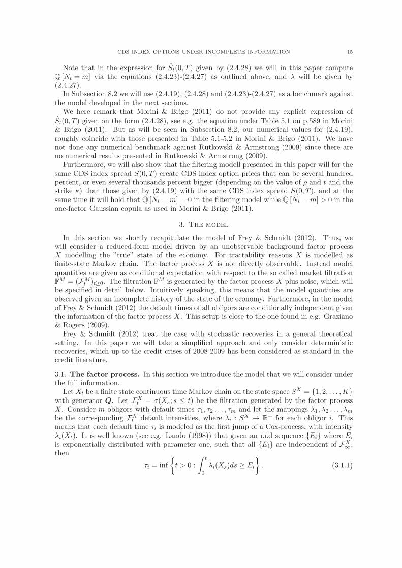
3. The model

In this section we shortly recapitulate the model of Frey & Schmidt (2012). Thus, wewill consider a reduced-form model driven by an unobservable background factor processX modelling the ”true” state of the economy. For tractability reasons X is modelled asfinite-state Markov chain. The factor process X is not directly observable. Instead modelquantities are given as conditional expectation with respect to the so called market filtrationFM = (FM

t )t≥0. The filtration FM is generated by the factor process X plus noise, which willbe specified in detail below. Intuitively speaking, this means that the model quantities areobserved given an incomplete history of the state of the economy. Furthermore, in the modelof Frey & Schmidt (2012) the default times of all obligors are conditionally independent giventhe information of the factor process X. This setup is close to the one found in e.g. Graziano& Rogers (2009).

Frey & Schmidt (2012) treat the case with stochastic recoveries in a general theoreticalsetting. In this paper we will take a simplified approach and only consider deterministicrecoveries, which up to the credit crises of 2008-2009 has been considered as standard in thecredit literature.

3.1. The factor process. In this section we introduce the model that we will consider underthe full information.

LetXt be a finite state continuous time Markov chain on the state space SX = 1, 2, . . . ,Kwith generator Q. Let FX

t = σ(Xs; s ≤ t) be the filtration generated by the factor processX. Consider m obligors with default times τ1, τ2 . . . , τm and let the mappings λ1, λ2 . . . , λm

be the corresponding FXt default intensities, where λi : S

X 7→ R+ for each obligor i. Thismeans that each default time τi is modeled as the first jump of a Cox-process, with intensityλi(Xt). It is well known (see e.g. Lando (1998)) that given an i.i.d sequence Ei where Ei

is exponentially distributed with parameter one, such that all Ei are independent of FX∞,

then

τi = inf

t > 0 :

∫ t

0λi(Xs)ds ≥ Ei

. (3.1.1)


Hence, for any T ≥ t we have

Q[τi > t | FX

T

]= exp

(−∫ t

0λi(Xs)ds

)(3.1.2)

and thus

Q [τi > t] = E

[exp

(−∫ t

0λi(Xs)ds

)]. (3.1.3)

Note that the default times are conditionally independent, given FX∞.

The states in SX = 1, 2, . . . ,K are ordered so that state 1 represents the best state andK represents the worst state of the economy. Consequently, the mappings λi(·) are chosen tobe strictly increasing in k ∈ 1, 2, . . . ,K, that is λi(k) < λi(k+1) for all k ∈ 1, 2, . . . ,K−1and for every obligor in the portfolio.

3.2. The market filtration and full information. In this subsection we formally introducethe market filtration, that is the information observed by the market participants. Recallthat the prices of all securities are given as conditional expectations with respect to thisfiltration. We also shortly discuss the full information F = (Ft)t≥0, which is the biggestfiltration containing all other filtrations, where (Ω,G,P) with G = F∞ will be the underlyingprobability space assumed in the rest of this paper.

Let Yt,i denote the random variable Yt,i = 1τi≤t and Yt be the vector Yt = (Yt,1, . . . , Yt,m).

The filtration FYt = σ(Ys; s ≤ t) represents the default portfolio information at time t,

generated by the process (Ys)s≥0. Furthermore, let Bt be a one-dimensional Brownian motionindependent of (Xt)t≥0 and (Yt)t≥0 and let a(·) be a function from 1, 2, . . . ,K to R. Next,define the process Zt as

Zt =

∫ t

0a(Xs)ds +Bt. (3.2.1)

We here remark that Frey & Schmidt (2012) allows for multivariate Brownian motion Bt

in (3.2.1) as well as a vector valued mapping a(·) with same dimension as Bt and in thenumerical studies of Frey & Schmidt (2012) they use a one-dimensional Brownian motion Bt.In this paper we restrict ourselves to only one source of randomness in the noise representation(3.2.1). Extending to several sources of randomness in (3.2.1) will in principle not change themain ideas in this paper. Intuitively Zt represents the noisy history of Xt and the functionalform of Zt given by (3.2.1) is a representation that is standard in the nonlinear filteringtheory, see e.g. Davis & Marcus (1981). Following Frey & Schmidt (2012), we define themarket filtration FM = (FM

t )t≥0 as

FMt = FY

t ∨ FZt . (3.2.2)

We set the full information F = (Ft)t≥0 to be the biggest filtration containing all otherfiltrations with G = F∞. We can for example let Ft be given by

Ft = FXt ∨ FY

t ∨ FBt (3.2.3)

where (FBt )t≥0 is the filtration generated by the Brownian motion Bt. Note that FX

t is nota subfiltration of FZ

t , and similarly, FBt is not contained in FZ

t .


4. Applying the Kushner-Stratonovic SDE in the credit risk model

In this section we study the Kushner-Stratonovic SDE in our filtering model. We use thesame notation as in Frey & Schmidt (2012). First, define πk

t as the conditional probability ofthe event Xt = k given the market information FM

t at time t, that is

πkt = Q

[Xt = k | FM

t

](4.1)

and let πt ∈ RK be a row-vector such that πt =(π1t , . . . , π

Kt

). In the sequel, for any Ft-

adapted process Ut we let Ut denote the optional projection of Ut onto the filtration FMt , that

is Ut = E[Ut | FM

t

]. To this end, we have for example

λi(Xt) = E[λi(Xt) | FM

t

]=

K∑

k=1

λi(k)πkt

a(Xt) = E[a(Xt) | FM

t

]=

K∑

k=1

a(k)πkt .

Next, define Mt,i and µt as

Mt,i = Yt,i −∫ t∧τi

0

λi(Xs−)ds for i = 1, . . . ,m (4.2)

µt = Zt −∫ t

0a(Xs) ds

In Frey & Schmidt (2012) it is shown that Mt,i is an FMt -martingale, for i = 1, 2, . . . ,m

and that µt is a Brownian motion with respect to the filtration FMt . Thus, the vector

Mt = (Mt,1, . . . ,Mt,m) is an FMt -martingale. These results have been proven previously

when considered separately, i.e. for pure diffusion filtering problems, see e.g. Davis & Marcus(1981), and pure jump process filtering process, see e.g Bremaud (1981).

Furthermore, Frey & Schmidt (2012) also proves the following proposition, which is aversion of the Kushner- Stratonovic equations, adopted to the filtering models presented inthis paper (originally developed in Frey & Schmidt (2012)).

Proposition 4.1. With notation as above, the processes πkt satisfies the following K-dimensional

system of SDE-s,

dπkt =

K∑

ℓ=1

Qℓ,kπℓtdt+ (γk(πt−))

⊤ dMt + αk(πt) dµt , (4.3)

where (γk(π))⊤ =(γk1 (π), . . . , γ

km(π)

)with π = (π1, π2, . . . , πm) and the coefficients γki (π)

are mappings given by

γki (π) = πk( λi(k)∑K

n=1 λi(n)πn− 1), 1 ≤ i ≤ m (4.4)

and

αk(πt) = πkt

(a(k)−

K∑

n=1

πnt a(n)

), 1 ≤ k ≤ K. (4.5)


TheK-dimensional SDE-system partly uses the vector notation for theMt vector. However,as will be seen below, it will be beneficial to rewrite this SDE on component form, especiallywhen we consider homogeneous credit portfolios. Thus, let us rewrite (4.3) on componentform, so that

dπkt =

K∑

ℓ=1

Qℓ,kπℓtdt+

m∑

i=1

γki (πt−)dMt,i + αk(πt)dµt. (4.6)

Next, let us consider a homogeneous credit portfolio, that is, all obligors are exchangeable sothat λi(Xt) = λ(Xt) and γki (πt) = γk(πt) for each obligor i and define Nt as

Nt =m∑

i=1

Yt,i =m∑

i=1

1τi≤t. (4.7)

Furthermore, define λ as λ = (λ(1), . . . , λ(K)) and let ek ∈ Rm be a row vector where theentry at position k is 1 and the other entries are zero. For a homogeneous portfolio the resultsof Proposition 4.1 can be simplified to the following corollary.

Corollary 4.2. Consider a homogeneous credit portfolio with m obligors. Then, with notation

as above, the processes πkt satisfy the following K-dimensional system of SDE-s,

dπkt = γk(πt−)dNt + πt−

(Qe⊤k − γk(πt−)λ

⊤ (m−Nt))dt+ αk(πt)dµt (4.8)

where γk(πt) and αk(πt) are given by

γk(πt) = πkt

(λ(k)

πtλ⊤− 1

)and αk(πt) = πk

t

(a(k) −

K∑

n=1

πnt a(n)

). (4.9)

Proof. First, from (4.2) we have dMt,i = dYt,i−1τi>tλi(Xt)dt = dYt,i−1τi>t

∑Kk=1 λi(k)π

kt dt

which in (4.6) implies that

dπkt = πtQe⊤k dt+

m∑

i=1

γki (πt−)dYt,i −m∑

i=1

γki (πt−)1τi>t

K∑

k=1

λi(k)πkt dt+ αk(πt)dµt. (4.10)

Since λi(Xt) = λ(Xt) and γki (πt) = γk(πt) for all obligors i, and recalling that Nt denotesNt =

∑mi=1 Yt,i =

∑mi=1 1τi≤t so that

∑mi=1 1τi>t = m−Nt, we can after some computations

rewrite (4.10) as

dπkt = γk(πt−)dNt + πt−

(Qe⊤k − γk(πt−)λ

⊤ (m−Nt))dt+ αk(πt)dµt

where γk(πt) and αk(πt) are given by γk(πt) = πkt

(λ(k)

πtλ⊤ − 1

)and αk(πt) = πk

t

(a(k) −

∑Kn=1 π

nt a(n)

).

From the SDE (4.8) in Corollary 4.2 we clearly see that the dynamics of the conditionalprobabilities πk

t contains a drift part, a diffusion part and a jump part. The diffusion part isdue to the dµt component and the jump part is due to the defaults in the portfolio, given bythe differential dNt.

Figure 2 visualizes a simulated path of π1t given by (4.8) in Corollary 4.2 in an example

where K = 2 and m = 125, using fictive parameters for Q and λ assuming a(k) = c · lnλ(k)for a constant c. From the third Figure 2 we clearly see that π1

t has jump, drift and diffusionparts. The first and second subfigures in Figure 2 shows the corresponding trajectories for Xt


0 0.5 1 1.5 2 2.5 31

1.5

2

time t

the

proc

ess

Xt

A realization of the process Xt

Xt

0 0.5 1 1.5 2 2.5 30

10

20

time t

the

defa

ult p

roce

ss N

t

A realization of the point process Nt

Nt

0 0.5 1 1.5 2 2.5 30

0.5

1

time (in years)

the

prob

abili

ty π

t1

A trajectory of πt1 simulated with the Kushner−Strataonovich SDE

πt1

Figure 2. A simulated trajectory of Xt, Nt and π1

twhere K = 2 and m = 125.

and Nt. Note how the defaults presented by Nt cluster as Xt switches to state 2, representingthe worse economic state among 1, 2.

5. The main building blocks

In this section we describe the main building blocks that will be necessary to find formulasfor portfolio credit derivatives such as e.g. the CDS index. Examples of such building blocksare the conditional survival distribution, the conditional number of defaults and the condi-tional loss distribution. The conditional expectations are with respect to the market informa-tion FM

t defined in Equation (3.2.2) in Subsection 3.2. Recall that Yt,i denotes the randomvariable Yt,i = 1τi≤t, Yt = (Yt,1, . . . , Yt,m) and Nt and Lt are given by Nt =

∑mi=1 1τi≤t

and Lt =1m

∑mi=1(1− φi)1τi≤t where φi is the recovery rate for obligor i. Our main task in

this section is to find the following quantities

Q[τi > T | FM

t

], E

[NT | FM

t

]and E

[LT | FM

t

]

where T > t. These expressions will be useful when deriving formulas for the CDS indexspread S(t, T ) as well as the CDS index option discussed in Section 6.

5.1. The conditional survival distribution. In this subsection we study the conditionalsurvival distribution Q

[τi > T | FM

t

]for T > t in the filtering model. To do this we need to

introduce some notation. If Xt is a finite state Markov jump process on SX = 1, 2, . . . ,K


with generator Q, then, for a function λ(x) : SX 7→ R we denote the matrix Qλ = Q − Iλ

where Iλ is a diagonal-matrix such that (Iλ)k,k = λ(k). Furthermore, we let 1 be a column

vector in RK where all entries are 1. The following theorem is a perquisite for all other resultsin this paper and is therefore a core result.

Theorem 5.1. Consider a credit portfolio specified as in Section 3 and let λi(Xt) be the

FXt -intensity for obligor i. If T ≥ t then, with notation as above

Q[τi > T | FM

t

]= 1τi>tπte

Qλi(T−t)

1 (5.1.1)

where the matrix Qλi= Q− Iλi

is defined as above.

Proof. Since T > t, then

E[1τi>T

∣∣Ft

]= E

[1τi>T

∣∣FXt ∨ FYi

t

]= 1τi>tE

[e−

∫T

tλi(Xs)ds

∣∣∣FXt

](5.1.2)

where the first equality is due to the fact that conditionally on X, then τi is independent ofτj for j 6= i. The second equality follows from a standard result for the first jump time of aCox-process, see e.g. p.102 in Lando (1998), Corollary 9.1 in McNeil et al. (2005) or Corollary6.4.2 in Bielecki & Rutkowski (2001). Since T > t and due to the Markov property of X we

can rewrite the quantity E[e−

∫T

tλi(Xs)ds

∣∣∣FXt

]as

E[e−

∫T

tλi(Xs)ds

∣∣∣FXt

]= E

[e−

∫T

tλi(Xs)ds

∣∣∣Xt

]=

K∑

k=1

E[e−

∫T

tλi(Xs)ds

∣∣∣Xt = k]1Xt=k

which implies that (recall that FXt is not a subfiltration of FM

t )

E[E[e−

∫T

tλi(Xs)ds

∣∣∣FXt

] ∣∣∣FMt

]=

K∑

k=1

E[e−

∫T

tλi(Xs)ds

∣∣∣Xt = k]πkt (5.1.3)

where we used the notation πkt = Q

[Xt = k | FM

t

]. By using Theorem A.1 in Appendix A

we have that

E[e−

∫T

tλi(Xs)ds

∣∣∣Xt = k]= eke

Qλi

(T−t)1 (5.1.4)

where the matrix Qλiis defined as previously. So (5.1.4) in (5.1.3) yields

E[E[e−

∫T

tλi(Xs)ds

∣∣∣FXt

] ∣∣∣FMt

]=

K∑

k=1

ekeQ

λi(T−t)

1πkt = πte

Qλi

(T−t)1 (5.1.5)

where we recall that πt is a row-vector such that πt =(π1t , . . . , π

Kt

). Next, note that

E[1τi>T

∣∣FMt

]= E

[E[1τi>T

∣∣Ft

] ∣∣FMt

]

= 1τi>tE[E[e−

∫T

tλi(Xs)ds

∣∣∣FXt

] ∣∣∣FMt

]

= 1τi>tπteQλi

(T−t)1

where the second equality is due to (5.1.2) and the third equality follows from (5.1.5). Thus,

for T ≥ t we conclude that Q[τi > T | FM

t

]= 1τi>tπte

Qλi(T−t)

1 which proves the theorem.


Theorem 5.1 allows us to state credit related derivatives quantizes in very compact andcomputational convenient formulas, as will seen later in this paper. We also remark thatTheorem 5.1 has previously been successfully used in Herbertsson & Frey (2014) in which thetheorem was stated without a proof, see Theorem 3.1 p. 1416 in Herbertsson & Frey (2014).Instead Herbertsson & Frey (2014) refers to the proof of Theorem 5.1 in an earlier version ofthis paper.

5.2. The conditional number of defaults. In this subsection we derive practical expres-sions for E

[Nt | FM

t

]. We consider an homogeneous credit portfolios where λi(Xt) = λ(Xt)

so that Qλi= Qλ for each obligor i. Recall that Nt =

∑mi=1 1τi≤t. The main message of

this subsection is the following proposition.

Proposition 5.2. Consider an exchangeable credit portfolio with m obligors in a model spec-

ified as in Section 3. Then, for T ≥ t and with notation as above

E[NT | FM

t

]= m− (m−Nt)πte

Qλ(T−t)1. (5.2.1)

Proof. Let T > t and first note that

E [NT | Ft] = m−m∑

i=1

E[1τi>T

∣∣Ft

]= m−

m∑

i=1

1τi>tE[e−

∫T

tλi(Xs)ds

∣∣∣FXt

](5.2.2)

where the last equality is due to Equation (5.1.2) in Theorem 5.1. Furthermore, in a ho-mogeneous portfolio we have λi(Xs) = λ(Xs) for all obligors i and this in (5.2.2) implies

that E [NT | Ft] = m − (m−Nt)E[e−

∫T

tλ(Xs)ds

∣∣∣FXt

]. Thus, by using E

[NT | FM

t

]=

E[E [NT | Ft] | FM

t

]and following similar arguments as in Theorem 5.1 we conclude after

some computations that E[NT | FM

t

]= m − (m−Nt)πte

Qλ(T−t)1 which proves the propo-sition.

A similar proof can be found for inhomogeneous portfolios.

5.3. The conditional portfolio loss: The case with constant recovery. This is trivialfor homogeneous portfolios, given the results from Subsection 5.2. To see this, recall thatNt =∑m

i=1 1τi≤t and Lt =1m

∑mi=1(1 − φi)1τi≤t where φi are constants and in a homogeneous

portfolio we have φ1 = φ2 = . . . = φm = φ so that Lt =(1−φ)m

Nt. Thus,

E[LT | FM

t

]=

(1− φ)

mE[NT | FM

t

](5.3.1)

where E[NT | FM

t

]is explicitly given in Subsection 5.2 for homogeneous portfolios. To be

more specific, (5.3.1) with Proposition 5.2 yields

E[LT | FM

t

]= (1− φ)

(1−

(1− Nt

m

)πte

Qλ(T−t)1

). (5.3.2)

Similar results can also be obtained in an inhomogeneous portfolio both with identical ordifferent recoveries.


6. The CDS index in the filtering model

In this section we apply the results from Section 5 together with Subsection 2.2 to findformulas for the CDS index spreads in the models introduced in Section 3. This will be donein a homogeneous portfolio. We will assume that the risk free interest rate is constant andgiven by r and for t < s we let B(t, s) denote B(t, s) = e−r(s−t). We can now state thefollowing theorem.

Theorem 6.1. Consider a CDS index portfolio in the filtering model. Then, with notation

as above

DL(t, T ) = E

[∫ T

t

B(t, s)dLs

∣∣∣∣FMt

]=

(1− Nt

m

)πtA(t, T )1 (6.1)

and

PV (t, T ) = E[VP (t, T ) | FM

t

]=

(1− Nt

m

)πtB(t, T )1 (6.2)

where A(t, T ) and B(t, T ) are defined as

A(t, T ) = (1− φ)

[I − eQλ(T−t)

(I + r (Qλ − rI)−1

)e−r(T−t) + r (Qλ − rI)−1

](6.3)

B(t, T ) =1

4

⌈4T ⌉∑

n=nt

eQλ(tn−t)e−r(tn−t). (6.4)

Furthermore, if Nt < m we have

S(t, T ) =πtA(t, T )1

πtB(t, T )1. (6.5)

Proof. First we recall the definitions of DL(t, T ), PV (t, T ) and S(t, T ) from (2.2.3), (2.2.4),(2.2.5) and (2.2.6) with the difference that we now replace Ft with FM

t given by (3.2.2).

Next, the term∫ T

tB(t, s)dLs used in DL(t, T ) can be rewritten in a more practical form using

integration by parts (see e.g. Theorem 3.36, p.107 in Folland (1999)), so that∫ T

tB(t, s)dLs =

B(t, T )LT − Lt +∫ T

trB(t, s)Lsds and by applying Fubini-Tonelli on this expressions then

renders

E

[∫ T

t

B(t, s)dLs

∣∣∣∣FMt

]= B(t, T )E

[LT | FM

t

]− Lt +

∫ T

t

rB(t, s)E[Ls | FM

t

]ds. (6.6)

Furthermore, if s > t then (5.3.2) gives

E[Ls | FM

t

]= (1− φ)

(1−

(1− Nt

m

)πte

Qλ(s−t)1

)

so using this in (6.6) and recalling that B(t, s) = e−r(s−t) for s > t, we get

E

[∫ T

t

B(t, s)dLs

∣∣∣∣FMt

]= B(t, T )E

[LT | FM

t

]− Lt +

∫ T

t

rB(t, s)E[Ls | FM

t

]ds

= e−r(T−t)(1− φ)

(1−

(1− Nt

m

)πte

Qλ(T−t)1

)− (1− φ)

mNt

+

∫ T

t

re−r(s−t)(1− φ)

(1−

(1− Nt

m

)πte

Qλ(s−t)1

)ds.

(6.7)


The integral in the RHS of (6.7) can be simplified according to∫ T

t

re−r(s−t)(1− φ)

(1−

(1− Nt

m

)πte

Qλ(s−t)1

)ds

= (1− φ)(1− e−r(T−t)

)

− r(1− φ)

(1− Nt

m

)πt

(eQλ(T−t)e−r(T−t) − I

)(Qλ − rI)−1

1

(6.8)

where the last equality in (6.8) is due to the fact that∫ T

t

e−r(s−t)eQλ(s−t)ds =

∫ T

t

e(Qλ−rI)(s−t)ds =(eQλ(T−t)e−r(T−t) − I

)(Qλ − rI)−1 .

Note that (Qλ − rI)−1 exists since Qλ − rI by construction is a diagonal dominant matrix,implying that det (Qλ − rI) 6= 0 by the Levy-Desplanques Theorem. By plugging (6.8) into(6.7) and performing some trivial but tedious computations we get

E

[∫ T

t

B(t, s)dLs

∣∣∣∣FMt

]

= (1− φ)

(1− Nt

m

)(1− πt

(eQλ(T−t)

(I + r (Qλ − rI)−1

)e−r(T−t) − r (Qλ − rI)−1

)1)

= (1− φ)

(1− Nt

m

)πt

[I − eQλ(T−t)

(I + r (Qλ − rI)−1

)e−r(T−t) + r (Qλ − rI)−1

]1

=

(1− Nt

m

)πtA(t, T )1

where we in the second equality used that 1 = πt1 = πtI1 and where A(t, T ) in the finalequality is given by

A(t, T ) = (1− φ)

[I − eQλ(T−t)

(I + r (Qλ − rI)−1

)e−r(T−t) + r (Qλ − rI)−1

]

which proves (6.1) and (6.3) where we also used (2.2.4) with Ft replaced by FMt given in

(3.2.2). To derive the expression for the premium leg we use (5.2.1) in Proposition 5.2 with

s > t and obtain 1 − 1mE[Ns | FM

t

]=(1− Nt

m

)πte

Qλ(s−t)1 which in Equation (2.2.5), with

Ft replaced by FMt , then renders that

PV (t, T ) =1

4

⌈4T ⌉∑

n=nt

B(t, tn)

(1− 1

mE[Ntn | FM

t

])=

1

4

(1− Nt

m

) ⌈4T ⌉∑

n=nt

πteQλ(tn−t)1e−r(tn−t)

=

(1− Nt

m

)πtB(t, T )1

where B(t, T ) = 14

∑⌈4T ⌉n=nt

eQλ(tn−t)e−r(tn−t) and this proves (6.2) and (6.4). Finally, (6.5)follows from the definition in (2.2.6) together with the expressions for the default leg andpremium leg in (6.1) and (6.2).

Note that the term 1 − Nt/m in the right hand side of both (6.1) and (6.2) implies thatthe conditional expectations of the default and premium legs will be zero for the armageddonevent Nt = m. This fact is in line with the conclusion in (2.3.3) which holds for any model of


the default times τ1, . . . , τm. Furthermore, note that the right hand side in (6.5) is still welldefined when Nt = m.

From Theorem 6.1 we conclude that given the vector πt, then the formulas for the defaultand premium leg in the filtering model as well as the CDS index spread S(t, T ) are compactand computationally tractable closed-form expressions in terms of πt and Qλ. Furthermore,Theorem 6.1 will also help us to find tractable formulas for the payoff of more exotic derivativeswith the CDS index as a underlyer. Example of such derivatives are call options on the CDSindex, which we will treat in the next section.

7. CDS index options in the filtering model

In this section we apply the results from Section 6 and Subsection 2.3 to present a highlycomputationally tractable formula for the payoff of a so called CDS index option in the modelpresented in Section 3. Furthermore, we derive a lower bound for price of the CDS indexoption and also provide explicit conditions on the strike spread for which this inequalitybecomes an equality. The lower bound is computationally tractable and do not depend onany of the ”noise” parameters in the filtering model introduced in Section 3. Finally, weoutline how to explicitly compute the quantities involved in the lower bound for the price ofthe CDS index option.

By inserting the explicit expressions for the default and premium legs for the index-CDSspread given by (6.1) and (6.2) in Theorem 6.1 into the expression of the payoff Π(t, T ;κ) forthe CDS index option in Equation (2.3.5), that is

Π(t, T ;κ) = (DL(t, T )− κPV (t, T ) + Lt)+ .

we immediately make the payoff Π(t, T ;κ) very explicit in terms of πt, Nt, A(t, T ) andB(t, T ), as summarized in the following lemma.

Lemma 7.1. Consider a CDS index portfolio in the filtering model. Then, the payoff

Π(t, T ;κ) for an CDS index option with strike κ, exercise date t and maturity T for the

underlying CDS index, is given by

Π(t, T ;κ) =

(πt

[A(t, T )− κB(t, T )

]1

(1− Nt

m

)+

(1− φ)Nt

m

)+

(7.1)

where A(t, T ) and B(t, T ) are defined as in Theorem 6.1.

Note that on the event Nt = m, the right-hand side in (7.1) reduces to the randomvariable (1− φ)1Nt=m for any strike spread κ, which is consistent with Equation (2.3.7).

In view of Lemma 7.1 and since the price of the CDS index option C0(t, T ;κ) at time 0(i.e. today) is given by C0(t, T ;κ) = E

[e−rtΠ(t, T ;κ)

]we therefore get

C0(t, T ;κ) = e−rtE

[(πt

[A(t, T )− κB(t, T )

]1

(1− Nt

m

)+

(1− φ)Nt

m

)+]. (7.2)

Since no closed formulas are known for the entries in the vector πt it is difficult to findanalytical expressions for the formulas in the RHS of Equation (7.2). Instead we rely onMonte Carlo simulations of the filtering probabilities πt together with the compact formulafor the payoff function Π(t, T ;κ) given in (7.1).


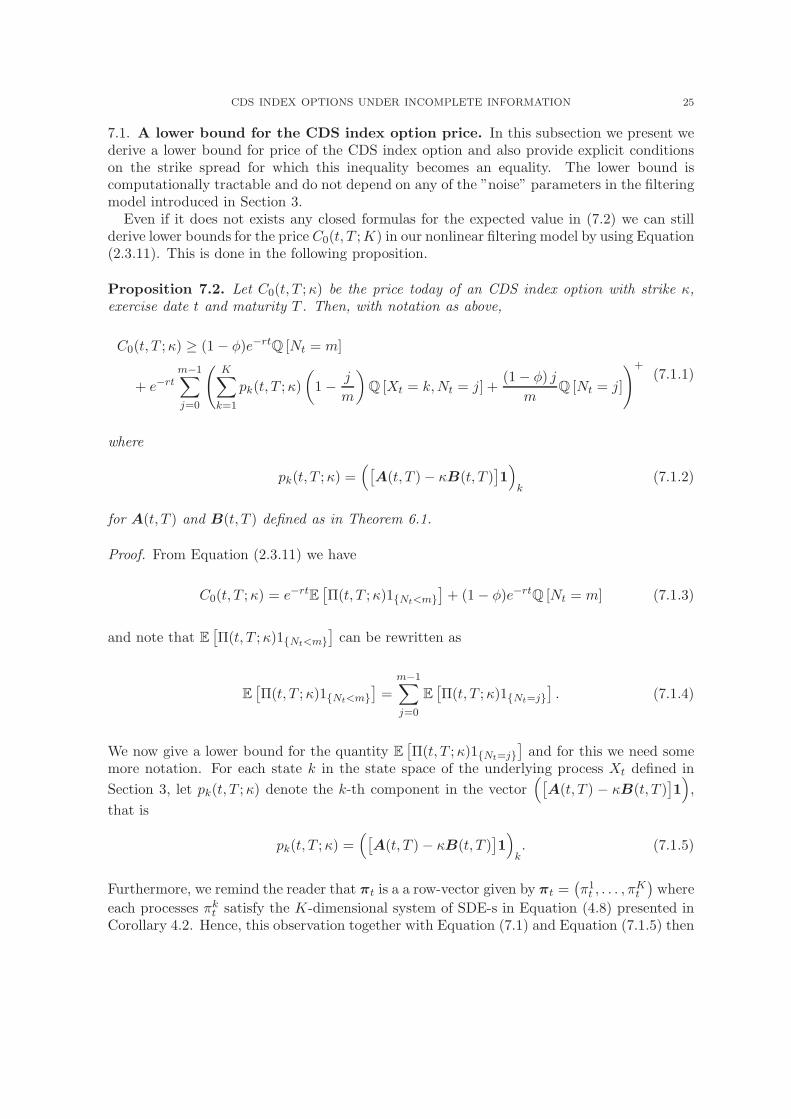
7.1. A lower bound for the CDS index option price. In this subsection we present wederive a lower bound for price of the CDS index option and also provide explicit conditionson the strike spread for which this inequality becomes an equality. The lower bound iscomputationally tractable and do not depend on any of the ”noise” parameters in the filteringmodel introduced in Section 3.

Even if it does not exists any closed formulas for the expected value in (7.2) we can stillderive lower bounds for the price C0(t, T ;K) in our nonlinear filtering model by using Equation(2.3.11). This is done in the following proposition.

Proposition 7.2. Let C0(t, T ;κ) be the price today of an CDS index option with strike κ,exercise date t and maturity T . Then, with notation as above,

C0(t, T ;κ) ≥ (1− φ)e−rtQ [Nt = m]

+ e−rt

m−1∑

j=0

(K∑

k=1

pk(t, T ;κ)

(1− j

m

)Q [Xt = k,Nt = j] +

(1− φ) j

mQ [Nt = j]

)+(7.1.1)

where

pk(t, T ;κ) =([

A(t, T )− κB(t, T )]1)k

(7.1.2)

for A(t, T ) and B(t, T ) defined as in Theorem 6.1.

Proof. From Equation (2.3.11) we have

C0(t, T ;κ) = e−rtE[Π(t, T ;κ)1Nt<m

]+ (1− φ)e−rtQ [Nt = m] (7.1.3)

and note that E[Π(t, T ;κ)1Nt<m

]can be rewritten as

E[Π(t, T ;κ)1Nt<m

]=

m−1∑

j=0

E[Π(t, T ;κ)1Nt=j

]. (7.1.4)

We now give a lower bound for the quantity E[Π(t, T ;κ)1Nt=j

]and for this we need some

more notation. For each state k in the state space of the underlying process Xt defined in

Section 3, let pk(t, T ;κ) denote the k-th component in the vector([

A(t, T ) − κB(t, T )]1),

that is

pk(t, T ;κ) =([

A(t, T )− κB(t, T )]1)k. (7.1.5)

Furthermore, we remind the reader that πt is a a row-vector given by πt =(π1t , . . . , π

Kt

)where

each processes πkt satisfy the K-dimensional system of SDE-s in Equation (4.8) presented in

Corollary 4.2. Hence, this observation together with Equation (7.1) and Equation (7.1.5) then


implies that we can rewrite the quantity E[Π(t, T ;κ)1Nt=j

]as follows

E[Π(t, T ;κ)1Nt=j

]= E

[(πt

[A(t, T )− κB(t, T )

]1

(1− j

m

)+

(1− φ) j

m

)+

1Nt=j

]

= E

(

K∑

k=1

πkt pk(t, T ;κ)

(1− j

m

)+

(1− φ) j

m

)+

1Nt=j

= E

(

K∑

k=1

πkt pk(t, T ;κ)

(1− j

m

)1Nt=j +

(1− φ) j

m1Nt=j

)+

≥(E

[K∑

k=1

πkt pk(t, T ;κ)

(1− j

m

)1Nt=j +

(1− φ) j

m1Nt=j

])+

(7.1.6)

where the last inequality is due to Jensens inequality. The quantity inside the max expressionon the last line in Equation (7.1.6) can be rewritten as

E

[K∑

k=1

πkt pk(t, T ;κ)

(1− j

m

)1Nt=j +

(1− φ) j

m1Nt=j

]

=K∑

k=1

pk(t, T ;κ)

(1− j

m

)E[πkt 1Nt=j

]+

(1− φ) j

mQ [Nt = j] .

(7.1.7)

Furthermore, since πkt = Q

[Xt = k | FM

t

]we have

E[πkt 1Nt=j

]= E

[Q[Xt = k | FM

t

]1Nt=j

]

= E[Q[Xt = k,Nt = j | FM

t

]]

= Q [Xt = k,Nt = j]

(7.1.8)

where the second equality follows from the fact that Nt is FMt -measurable since FM

t =FYt ∨FZ

t in view of Equation (3.2.2). Hence, inserting (7.1.8) in (7.1.7) and using (7.1.4) and(7.1.6), we retrieve the following lower bound for E

[Π(t, T ;κ)1Nt<m

]

E[Π(t, T ;κ)1Nt<m

]

≥m−1∑

j=0

(K∑

k=1

pk(t, T ;κ)

(1− j

m

)Q [Xt = k,Nt = j] +

(1− φ) j

mQ [Nt = j]

)+(7.1.9)

where pk(t, T ;κ) is given by Equation (7.1.5). Next, plugging (7.1.9) into (7.1.3) finally yieldsthe following lower bound for the option price C0(t, T ;κ),

C0(t, T ;κ) ≥ (1− φ)e−rtQ [Nt = m]

+ e−rt

m−1∑

j=0

(K∑

k=1

pk(t, T ;κ)

(1− j

m

)Q [Xt = k,Nt = j] +

(1− φ) j

mQ [Nt = j]

)+

which proves (7.1.1).


Thus, Proposition 7.2 establish a lower bound for the option price C0(t, T ;κ) as functionof the probabilities Q [Xt = k,Nt = j] and Q [Nt = j] for each state k and j = 0, 1, . . . ,m.Furthermore, we also remark that the quantity in the right hand side of (7.1.1) does notdepend on any of the ”noise” parameters in the filtering model introduced in Section 3.That is, the expression in the right hand side of (7.1.1) is independent of the mapping a :1, 2, . . . ,K 7→ Rl which is used in (3.2.1) to generate the noisy information FZ

t and thecorresponding noisy market information FM

t in (3.2.2), which in turn creates the nonlinearfiltering model introduced in Section 3.

The following corollary to Proposition 7.2 gives conditions for the possibilities of havingan equality in (7.1.1) instead of an inequality.

Corollary 7.3. Let C0(t, T ;κ) be the price today of an CDS index option with strike κ,exercise date t and maturity T . Then there exists a constant κ∗ such that for κ ≤ κ∗ it holds

C0(t, T ;κ) = (1− φ)e−rtQ [Nt = m]

+ e−rt

m−1∑

j=0

K∑

k=1

pk(t, T ;κ)

(1− j

m

)Q [Xt = k,Nt = j] + e−rt

m−1∑

j=0

(1− φ) j

mQ [Nt = j]

(7.1.10)

where κ∗ is given by

κ∗ = mink=1,...,K

κ∗k and κ∗k =ekA(t, T )1

ekB(t, T )1(7.1.11)

with A(t, T ), B(t, T ) and pk(t, T ;κ) defined as in Proposition 7.2.

Proof. First recall the option pricing formula (7.2)


[(πt

[A(t, T )− κB(t, T )

]1

(1− Nt

m

)+

(1− φ)Nt

m

)+](7.1.12)

where A(t, T ) and B(t, T ) are given as in Lemma 7.1. From Theorem A.1 in Appendix A,Proposition 5.2 and Equation (6.2) in Theorem 6.1 we conclude that ekB(t, T )1 ≥ 0 for eachstate k. Similarly, from the Equations (6.7) and (6.8) we also conclude that ekA(t, T )1 ≥ 0for every state k. Therefore, for each k the quantity

ek(A(t, T )− κB(t, T )

)1 = ekA(t, T )1− κekB(t, T )1 (7.1.13)

is the difference of two positive expressions when κ ≥ 0. Consequently, for each state k thereis a smallest strike spread denoted by κ∗k (bounded below by zero) for which the payoff in(7.1.13) is non-negative for all κ ≤ κ∗k. More explicit, κ∗k is defined by

κ∗k =ekA(t, T )1

ekB(t, T )1.

Furthermore, let κ∗ be

κ∗ = mink=1,...,K

κ∗k.

Then, by the construction of κ∗, we conclude that (7.1.13) is non-negative for all states k andall strike spreads κ where κ ≤ κ∗ which implies

πt

(A(t, T )− κB(t, T )

)1 ≥ 0 a.s. for κ ≤ κ∗, (7.1.14)


that is

Q[πt

(A(t, T )− κB(t, T )

)1 ≥ 0

]= 1 for κ ≤ κ∗.

By using (7.1.14) we conclude that the ”max” expression in (7.1.12) is superfluous for κ ≤ κ∗

and the option price C0(t, T ;κ) can then be rewritten as


[(πt

[A(t, T )− κB(t, T )

]1

(1− Nt

m

)+

(1− φ)Nt

m

)+]

= e−rtE

[πt

(A(t, T )− κB(t, T )

)1

(1− Nt

m

)+

(1− φ)Nt

m

]

= e−rtE

[πt

(A(t, T )− κB(t, T )

)1

(1− Nt

m

)]+ e−rt (1− φ)

mE [Nt] .

(7.1.15)

Furthermore, by following similar steps as in the Equations (7.1.7)-(7.1.8) we can rewrite the

expression E[πt

(A(t, T )− κB(t, T )

)1(1− Nt

m

)]as

E

[πt

(A(t, T )− κB(t, T )

)1

(1− Nt

m

)]=

m−1∑

j=0

K∑

k=1

pk(t, T ;κ)

(1− j

m

)Q [Xt = k,Nt = j]

(7.1.16)where pk(t, T ;κ) is defined as in (7.1.2). Note that

e−rt (1− φ)

mE [Nt] = (1− φ)e−rtQ [Nt = m] + e−rt

m−1∑

j=0

(1− φ) j

mQ [Nt = j] (7.1.17)

and this observation together with (7.1.16) in (7.1.15) for κ ≤ κ∗ then yields that

C0(t, T ;κ) = (1− φ)e−rtQ [Nt = m]

+ e−rt

m−1∑

j=0

K∑

k=1

pk(t, T ;κ)

(1− j

m

)Q [Xt = k,Nt = j] + e−rt

m−1∑

j=0

(1− φ) j

mQ [Nt = j]

which proves (7.1.12).

Note that Equation (7.1.10) in Corollary 7.3 is simply Equation (7.1.1) with a strict equalityand without a ”max” function for the second expression in the right hand side of (7.1.1). Wetherefore conclude that the inequality in (7.1.1) turns into a strict equality when the strikespread κ satisfies κ ≤ κ∗ with κ∗ defined as in (7.1.11).

It is remarkable that we in the noise model introduced in Section 3 for strike spreads κ suchthat κ ≤ κ∗ have derived an semi-explicit expression for the option price C0(t, T ;κ) givenby (7.1.10), which is independent of the mapping a : 1, 2, . . . ,K 7→ Rl used in (3.2.1) togenerate the noisy information FZ

t .

7.2. Auxiliary tools for computing the lower bounds. In this subsection we outlinehow to compute the quantizes involved in the lower bounds presented in Subsection 7.1. Theresults derived here are utilized in the implementations that are used in our numerical studiesin later sections of this paper.

Equation (7.1.1) in Proposition 7.2 provides a lower bound for the option price C0(t, T ;κ)as function of the probabilities Q [Xt = k,Nt = j] and Q [Nt = j] for each state k and j =0, 1, . . . ,m. Furthermore, (7.1.10) in Corollary 7.3 gives an exact expression for option price


C0(t, T ;κ) when κ ≤ κ∗ as function of Q [Xt = k,Nt = j] and Q [Nt = j]. Therefore we willbelow outline how to compute the probabilities Q [Xt = k,Nt = j] and Q [Nt = j] in our modelpresented in Section 3.

Consider a bivariate Markov process Ht on a state space SH defined as

SH = 1, . . . ,K × 0, 1, . . . ,m (7.2.1)

where |SH | = K(m + 1). So each state j ∈ SH can be written as a pair j = (k, j) where kand j are integers such that 1 ≤ k ≤ K and 0 ≤ j ≤ m. The first component of Ht belongsto 1, . . . ,K while the second component of Ht is defined on 1, . . . ,m. The intuitive ideabehind the bivariate Markov process Ht is of course that the first component of Ht should”mimic” the factor process Xt defined in Section 3.1 while the second component of Ht shouldrepresent Nt, i.e. the number of defaulted obligors in the portfolio at time t, as defined inprevious sections. More specific, for any pair (k, j) ∈ SH and for any time point t ≥ 0, wewant that the events Ht = (k, j) and Xt = k,Nt = j should have the same probabilityunder the risk-neutral measure Q, that is

Q [Ht = (k, j)] = Q [Xt = k,Nt = j] where (k, j) ∈ SH and t ≥ 0. (7.2.2)

In view of the above description of the bivariate Markov process Ht we now specify thegenerator QH for Ht on SH . For a fixed value k of the first component of Ht we can treatthe second component of Ht as a pure death process on 0, 1, . . . ,m, i.e. a process whichcounts the number of defaulted obligors in the portfolio given that the underlying economy isin state k, that is Xt = k. Therefore, for any j = 0, 1, . . . ,m−1 the process Ht can jump from(k, j) to (k, j+1) with intensity (m−j)λ(k) where the mapping λ(·) is defined as in Corollary4.2. Recall that λ(k) is the individual default intensity when the factor process is in statek, i.e. Xt = k. Next, for a fixed value j of the second component of Ht (i.e. the number ofdefaulted obligors at time t are j) consider two distinct states k and k′ in 1, . . . ,K. Then,inspired by the construction of the underlying factor process Xt with generator Q, we let thebivariate process Ht jump from (k, j) to (k′, j) with intensity Qk,k′ where k 6= k′. These arethe only allowed transitions for Ht. Hence, the generator QH for Ht is then given by

(QH)(k,j),(k,j+1) = (m− j)λ(k) 0 ≤ j ≤ m− 1, 1 ≤ k ≤ K

(QH)(k,j),(k′,j) = Qk,k′ 0 ≤ j ≤ m, 1 ≤ k, k′ ≤ K k 6= k′(7.2.3)

and for each pair k, j we also have that

(QH)(k,j),(k,j) = −∑

(k′,j′)∈SH ,k′ 6=k,j′ 6=j

(QH)(k,j),(k′,j′) . (7.2.4)

where the other entries in QH are zero. In view of this construction it is easy to see that itmust hold

Q [Ht = (k, j)] = Q [Xt = k,Nt = j] where (k, j) ∈ SH and t ≥ 0. (7.2.5)

Let αH ∈ RK(m+1) be the initial distribution of the Markov process Ht on the state spaceSH with generator QH and consider j ∈ SH . From Markov theory we know that

Q [Ht = j] = αHeQHtej , (7.2.6)

where ej ∈ RK(m+1) is a column vector where the entry at position j is 1 and the other entries

are zero. Furthermore, eQHt is the matrix exponential which has a closed form expression in


terms of the eigenvalue decomposition of QH . Thus, in view of (7.2.5) and (7.2.6) we havefor any j = (k, j) ∈ SH and t ≥ 0 that

Q [Xt = k,Nt = j] = αHeQHte(k,j). (7.2.7)

So (7.2.7) provides us with an efficient way to compute the probabilities Q [Xt = k,Nt = j]for any t ≥ 0 and any pair j = (k, j) where k and j are integers such that 1 ≤ k ≤ K and0 ≤ j ≤ m. Note that there exist over 20 different ways to compute the matrix exponential,for more on this see e.g in Moeler & Loan (1978) and Moeler & Loan (2003).

Since Q [Nt = j] =∑K

k=1Q [Xt = k,Nt = j] we retrieve that

Q [Nt = j] = αHeQH t

K∑

k=1

e(k,j) = αHeQH te(·,j) (7.2.8)

where e(·,j) ∈ RK(m+1) is a column vector defined as e(·,j) =∑K

k=1 e(k,j). Finally, let us

specify the the initial distribution αH ∈ RK(m+1) of the Markov process Ht on the statespace SH , defined as in (7.2.1). First, let α be the initial distribution of the process Xt

defined in Section 3.1. Then αk = Q [X0 = k] but we also know that

πk0 = Q

[X0 = k | FM

0

]= Q [X0 = k] = αk (7.2.9)

which gives a relation between the values πk0 and αk. Next, let us now the initial distribution

αH ∈ RK(m+1). We assume that all obligors in the portfolio are ”alive” (non-defaulted) attime t = 0, i.e. today, which implies that the second component must be zero for all statesof the economy background process modelled by the first component of the bivariate Markovprocess. Hence, it must hold that

K∑

k=1

(αH)(k,0) = 1 and (αH)(k,j) = 0 for j = 1, 2, . . . ,m (7.2.10)

which in turn guarantees that the sum of the entries in αH are one.By using the formulas (7.2.7), (7.2.8) and (7.2.10) in (7.1.1) we can efficiently compute

numerical values for the lower bounds of the option price C0(t, T ;κ). Similarly, using (7.2.7),(7.2.8) and (7.2.10) in (7.1.10) will render exact values of the option price C0(t, T ;κ) whenκ ≤ κ∗ where κ∗ is defined as in (7.1.11).

Since typically m and K are allowed to be large, especially m, we will in general deal withvery high dimensional state spaces of size (m+1)×K, which requires special treatment whennumerically dealing with the matrix exponential of the generator for Ht. Just computingthe matrix exponential with standard algorithms will make the implementation slow and alsoinaccurate. Instead we will rely on the so-called uniformization method which has successfullybeen utilized in high-dimensional state space applications of portfolio credit risk, see e.g. inHerbertsson (2007), Herbertsson & Rootzen (2008), Herbertsson (2011), Bielecki, Crepey &Herbertsson (2011) and Lando (2004). In our case we will also exploit the sparseness of thetransition matrices for Ht which makes the running times even quicker. With the help ofHt we will also display the loss distribution Q [Nt = k] for k = 0, 1, . . . ,m and in particularthe armageddon probabilities Q [Nt = m] for some calibrated examples in the filtering modeloutlined in Section 3 - 7. Finally, we have also performed robustness testes in order to increasethe reliability of the implemented code. For example, we have checked that Q [Xt = k] is thesame via Q and QH .


8. Numerical studies

In this section we perform various numerical studies of the CDS index spread and CDSindex option prices presented in Section 6 and 7, which in turn are based on the filtering modeloutlined in Section 3. The numerical studies are performed by calibration all parameters tomarket data

First, in Subsection 8.1 we gives a detailed outline of how the matrix Q and vector λ arechosen and then discuss how to estimate/calibrate the parameters θ = (Q,λ, a(x)) in thefiltering model introduced in Section 3 - 7.

Next, in Subsection 8.2 we use the results of Subsection 8.1 to calibrate, compute anddisplay the simulated CDS index option prices as well as the lower bounds derived in Section7 as functions of varies parameters such as the strike, the maturity and the spot-spread. Wealso calibrate the benchmark model 2.4.19 to the same spot CDS index spread. After this wecompare the filtering prices, their lower bound prices and the benchmark prises for differentvalues of ρ, σ and c. In particular, a numerical study is performed where we show that thelower bound in our model can be several hundred percent bigger compared with models whichassume that the CDS-spreads follows a log-normal process. Also a systematic study is donein order to understand the impact of various model parameters on CDS index options (andon the index itself)

8.1. Specifying the parameters and calibrating the filtering model. In this sectionwe discuss how to estimate/calibrate the parameters θ = (Q,λ, a(x)) in the filtering modelintroduced in Section 3. Recall that a(x) is the mapping used in (3.2.1) when constructingZt which is a function of Xt via the integral of the mapping a(Xt) plus noise in form of aBrownian motion. Just as in Herbertsson & Frey (2014) and Frey & Schmidt (2012) we useone source of randomness when modelling the noise and in this paper we choose the mappinga : 1, 2, . . . ,K 7→ R in (3.2.1) to be on the form

a(Xt) = c lnλ(Xt) that is a(k) = c lnλ(k) for each state k (8.1.1)

where c is a constant. The parametrization (8.1.1) have previously also been used in Herberts-son & Frey (2014), Frey & Schmidt (2012) and Frey & Schmidt (2011), see e.g. Subsection 5.3in Frey & Schmidt (2012) and Example 7.6.1 in Frey & Schmidt (2011). For a detailed motiva-tion of the choice (8.1.1) see on p.1420 in Herbertsson & Frey (2014). Hence, a(k) = c · ln λ(k)for a constant c, so the parameters θ to be estimated are then given by θ = (Q,λ, c).

Next, for λ = (λ(1), . . . , λ(K)) we will use the following piecewise linear parametrizationof the mapping λ(k) for the individual default intensity,

λ(k) =

bk if k ≤ ⌈K2 ⌉b⌈K2 ⌉(1− β) + βbk if k > ⌈K2 ⌉

(8.1.2)

where β and b are constants such that β > 1 and b > 0. Note that for a continuous versionof λ(·) we see that the left and right limit are the same which motivates the choice of theparameters for the case k > ⌈K2 ⌉, i.e. these are choosen so that

limx↑⌈K

2⌉λ(x) = lim

x↓⌈K

2⌉λ(x).

We here remind the reader that the states in SX = 1, 2, . . . ,K are ordered so that state1 represents the best state and K represents the worst state of the economy. Consequently,the mapping λ(·) is chosen to be strictly increasing in k ∈ 1, 2, . . . ,K. This implies that


β ≥ 1 in (8.1.2) and in our practical implementation we choose strict inequality, i.e. β > 1so that the slope of the line λ(k) will increase more for k > ⌈K2 ⌉ compared with k ≤ ⌈K2 ⌉.The parametrization of λ(k) in (8.1.2) is convenient in the sense that it describes the functionλ(k) with only two parameters β and b, regardless of the number of states K. The choice ofthe breakpoint ⌈K2 ⌉ can of course be changed, as well as the number of breakpoints, but morebreakpoints forces us to use more parameters when describing λ(k) (for a piecewise linearfunction we need a parameter for each slope in each region between the breakpoints etc.).

Next, we will assume that the finite state continuous time Markov chain Xt on the statespace SX = 1, 2, . . . ,K is a birth-death process with identical up and down transitionintensities given by q. Hence, the generator Q will satisfy

Qi,j =

q if i = j − 1 or i = j + 1−2q if 2 ≤ i = j ≤ K − 1−q if i = j = 1 or i = j = K0 otherwise

(8.1.3)

where q > 0. So (8.1.3) gives us only one parameter describing the generator Q regardless ofthe number of states K.

Hence, given the mapping a(x) in (8.1.1) and the parametrization of Q,λ in (8.1.2)-(8.1.3),the parameters to be estimated/calibrated are then θ = (b, β, q, c). In this paper we willestimate θ = (b, β, q, c) by calibrating the model spot CDS-index spread S(0, 5) towards thecorresponding observed market spread by using Equation (6.5) for t = 0 and the fact thatπ0 = α where α be the initial distribution of the process Xt defined in Section 3.1. Thismeans that we also need to find the K values of α = (α1, . . . , αK) and the parameters to beestimated are then θ = (b, β, q,α, c). By using (6.5) with π0 = α we define the T -year modelspot spread S(T ;θ) as

S(T ;θ) =αA(0, T )1

αB(0, T )1(8.1.4)

and θ = (b, β, q,α, c) is then calibrated via the following minimization routine

minθ

(S(T ;θ)− SM(T )

SM(T )

)2

subject to

α1 = 1

0 ≤ αk ≤ 1 for k = 1, . . . ,K

β > 1, b > 0, q > 0

(8.1.5)

where SM(T ) is the market quote for the T -year CDS-index spread today, i.e. at time t = 0.We here remark that we can extend the above calibration routine by including market CDS-index spreads SM (T )T∈T for a several maturities such as e.g. T ∈ T = 3, 5, 7, 10. Insuch a case the objective function in (8.1.5) is then replaced with

∑

T∈T

(S(T ;θ)− SM(T )

SM(T )

)2

.

We will in this paper only use one maturity T = 5 which historically has been the mostliquidly quoted CDS-index spread, in particular for the individual entries in the index.


The calibration of the parameters θ = (b, β, q,α, c) is thus a constrained nonlinear optimiza-tion problem and such routines are mostly solved numerically using standard mathematicalsoftware packages such as e.g. matlab. Numerical optimization routines typically requires theuser to provide an initial guess θ0 =

(b0, β0, q0,α

(0), c0)before running the scheme. In our

initial guess θ0 we let α(0)k = 1

Kfor each k.

Note that with t = 0 and for a given α, Equation (6.5), or equivalently (8.1.4) do not containthe parameter c used in (8.1.1). Hence, the calibration routine in (8.1.5) will not provide anestimation of c so this parameter must therefore be found by using another method.

If the mapping a(x) is on the form (8.1.1) one can estimate c, or more generally, the param-eters θ = (Q,λ, c) in several different ways. In Herbertsson & Frey (2014), which uses (8.1.1),the authors outline a novel approach for estimating the parameters θ = (Q,λ, c) in the fil-tering model of Frey & Schmidt (2012) under the physical/real measure by using time-seriesdata on a CDS index and classical maximum-likelihood algorithms. This calibration-approachnaturally incorporates the Kushner-Stratonovich SDE for the dynamics of the filtering prob-abilities. The computationally convenient formula for survival probability stated in Theorem5.1 is a prerequisite for the estimation algorithm in Herbertsson & Frey (2014). In Frey& Schmidt (2012) the authors calibrate the parameter c under the risk-neutral measure byusing the quadratic variation of the diffusion part of the index spread dynamics. Just asin Herbertsson & Frey (2014), the authors Frey & Schmidt (2012) observe that there wereno defaults within the iTraxx Europe in their observation period for the time series, so theempirical quadratic variation of the index spreads is an estimate of the continuous part of thequadratic variation on the same index spread. The value of c obtained in Frey & Schmidt(2012) is in the same order as the corresponding value of c found via the MLE-estimationin Herbertsson & Frey (2014) under the real measure, see Section 5 in Herbertsson & Frey(2014).

Herbertsson & Frey (2014) gives a short literature overview of some papers that develops es-timation techniques in models with incomplete information applied to credit risk applications.These are, amongst others Hurd & Zhou (2011), Azizpour, Giesecke & Kim (2011), Capponi& Cvitanic (2009), Fontana & Runggaldier (2010), Bhar & Handzic (2011), Duffie, Eckner,Horel & Saita (2009) and Koopman, Lucas & Schwaab (2011). Furthermore, Herbertsson &Frey (2014) also outline alternative methods to estimate θ = (Q,λ, c) using quadratic pro-gramming. We refer the reader to Herbertsson & Frey (2014) for more details on all of theabove topics.

In this paper the parameter c will be exogenously given and we can without loss of generalityassume that c has been estimated with some of the above mentioned methods. Nevertheless,we will perform numerical studies of the price C0(t, T ;κ) for an CDS index option in thefiltering model presented in Section 3 as function of e.g. the parameter c. In particularwe will use Monte-Carlos simulations to study C0(t, T ;κ) as functions of the parametersθ = (b, β, q,α) and c where (b, β, q,α) are obtained via the calibration (8.1.5). Furthermore,we will also investigate how far away the simulated prices will deviate from the lower bound ofthe price derived in Proposition 7.2. A numerical study of when the inequality in Proposition7.2 turns to the equality in given by Corollary 7.3 will also be performed.

8.2. Computing prices of options on the CDS index and their lower bound prices

and comparing with lognormal model prices. In this Subsection 8.2 we use the resultsof Subsection 8.1 to calibrate, compute and display the simulated CDS index option pricesas well as the lower bounds derived in Section 7 as functions of varies parameters such as


the strike, the maturity and the spot-spread. We also calibrate the benchmark model 2.4.19to the same spot CDS index spread. After this we compare the filtering prices, their lowerbound prices and the benchmark prises for different values of ρ, σ and c.

First, for m = 125, and r = 1% we calibrate both the filter modelling for K = 4 with theparametrization (8.1.2) via (8.1.5) and the benchmark model (2.4.19) via (2.4.27) against amarket spot CDS index spread S(0, 5) = 200 bp. Then we compute the option price (2.4.19)as function of the strike price κ for different maturities of t = 1, 3, 6, 9 months and differentvalues of ρ where ρ = 90%, 95% and ρ = 99.9 for σ = 113% and plot these values in Figure 3-5. In the same figures we also display lower bounds prices as function of κ when calibratedto the same market spot CDS index spread S(0, 5) = 200 bp. In all cases the we have thatφ = 40%. We also display the relative difference in percent between the option prices withoutabsolute value in the numerator, and where the denominator is the Morini-Brigo value. Inappendix we also show the difference between these prices without absolute value.

In Figure 3- 5 we clearly see that the lower bound in our model can be several hundred orthosands percent bigger compared with a model which assume that the CDS index spreadsfollows a log-normal process.

In Figure 3- 5 the volatility is kept constant. In order to view the impact of the volatilityσ, Figure 6 displays the Morini-Brigo option price 2.4.19 as function of the volatility σ forthe maturities t = 1, 3, 6, 9 months and correlations ρ = 90%, 95%, ρ = 99.9 where §(0, 5) =200, φ = 40% bp. In the same figure wa also pot the lower bound prices in the filtering modelcalibrated against the same spot spread S(0, 5) and same recovery, as well as the relativedifference in percent.

From the above studies we also discover that Q [Nt = m] = 0 for all studied scenarios in thispaper, and with the same market data such as spot-spread S(0, 5), maturity, interest rate, wewill show that the corresponding armageddon probability in the one-factor Gaussian copulamodel is much higher when the correlation parameter ρ goes to one. Despite this fact we willclearly see that the lower bounds for the CDS-index option prices in the filtering modell willalmost always be substantially higher (often several hundred percent higher) than the pricescomputed in the model Morini & Brigo (2011), at least for ”at-the-money” strike-spreads,i.e. when S(0, 5) = κ and the maturity is smaller or equal to 1.5 years. Only in extremescenarios, such as ρ ≥ 99.5% jointly with volatilizes σ ≥ 110% and maturities t ≥ 1.5 yearswill generate prices in Morini & Brigo (2011) that are slightly above the lower bounds for theCDS-index option prices in the filtering modell.


Strike spread κ (in bps) 0 100 200 300 400 500

pric

e (in

bps

)

0

500

1000t=1 months, T-t=5 years, S(0,5)=200 bp

Morini-Brigo prices, σ = 113 % , ρ = 90 %lower bound prices (filtering modell)


rela

tive

diff

(in %

)

0

1000

2000

3000

4000

relative difference


pric

e (in

bps

)

0

500




rela

tive

diff

(in %

)

-100

0

100

200

300

relative difference


pric

e (in

bps

)

0

500




rela

tive

diff

(in %

)

-20

0

20

40

60

80

relative difference


pric

e (in

bps

)

0

500




rela

tive

diff

(in %

)

-10

0

10

20

30

relative difference

Figure 3. The Morini-Brigo option prices for the maturities t = 1, 3, 6, 9 monthswhere ρ = 90%, σ = 113%, S(0, 5) = 200, φ = 40% bp and the lowerbound prices in the filtering model calibrated against the same spot spreadS(0, 5) and same recovery.



pric

e (in

bps

)

0

500




rela

tive

diff

(in %

)

0

1000

2000relative difference


pric

e (in

bps

)

0

500




rela

tive

diff

(in %

)

0

100

200 relative difference


pric

e (in

bps

)

0

500




rela

tive

diff

(in %

)

-20

0

20

40

60

80

relative difference


pric

e (in

bps

)

0

500




rela

tive

diff

(in %

)

-20

-10

0

10

20

30

relative difference

Figure 4. The Morini-Brigo option prices for the maturities t = 1, 3, 6, 9 monthswhere ρ = 95%, σ = 113%, S(0, 5) = 200, φ = 40% bp and the lowerbound prices in the filtering model calibrated against the same spot spreadS(0, 5) and same recovery.



pric

e (in

bps

)

0

500


Morini-Brigo prices, σ = 113 % , ρ = 99.9 %lower bound prices (filtering modell)


rela

tive

diff

(in %

)

-200

0

200

400

600

800

relative difference


pric

e (in

bps

)

0

500




rela

tive

diff

(in %

)

-50

0

50

100

150

relative difference


pric

e (in

bps

)

0

500




rela

tive

diff

(in %

)

-20

0

20

40

60

relative difference


pric

e (in

bps

)

0

500




rela

tive

diff

(in %

)

-40

-20

0

20

relative difference

Figure 5. The Morini-Brigo option prices for the maturities t = 1, 3, 6, 9 monthswhere ρ = 99.9%, σ = 113%, S(0, 5) = 200, φ = 40% bp and the lowerbound prices in the filtering model calibrated against the same spot spreadS(0, 5) and same recovery.


Volatility σ (in %) 0 20 40 60 80 100 120

pric

e (in

bps

)

0

100

200

300t=1 months, T-t=5 years, S(0,5)=200 bp, κ = 200 bp

Morini-Brigo prices, ρ = 90 %Morini-Brigo prices, ρ = 95 %Morini-Brigo prices, ρ = 99.9 %lower bound prices (filtering modell)

Volatility σ (in %) 0 20 40 60 80 100 120

rela

tive

diff

(in %

)

0

500

1000

1500

2000relative difference, ρ = 90 %relative difference, ρ = 95 %relative difference, ρ = 99.9 %

Volatility σ (in %) 0 20 40 60 80 100 120

pric

e (in

bps

)

0

100

200

300

400



Volatility σ (in %) 0 20 40 60 80 100 120

rela

tive

diff

(in %

)

0

200

400

600


Volatility σ (in %) 0 20 40 60 80 100 120

pric

e (in

bps

)

0

100

200

300

400



Volatility σ (in %) 0 20 40 60 80 100 120

rela

tive

diff

(in %

)

0

100

200

300


Volatility σ (in %) 0 20 40 60 80 100 120

pric

e (in

bps

)

100

200

300

400

500



Volatility σ (in %) 0 20 40 60 80 100 120

rela

tive

diff

(in %

)

0

100

200


Figure 6. The Morini-Brigo option prices as function of the volatility σ for the matu-rities t = 1, 3, 6, 9 months and correlations ρ = 90%, 95%, ρ = 99.9 whereS(0, 5) = 200, φ = 40% bp and the lower bound prices in the filteringmodel calibrated against the same spot spread S(0, 5) and same recovery.

References

Azizpour, S., Giesecke, K. & Kim, B. (2011), ‘Premia for correlated default risk’, Journal of Economic Dy-

namics and Control 35(8), 1340–1357.Bhar, R. & Handzic, N. (2011), ‘A multifactor model of credit spreads’, Asian-Pacific Financial Markets

18(1), 105–127.Bielecki, T. R., Crepey, S. & Herbertsson, A. (2011), Markov chain models of portfolio credit risk. Chapter 10

in ”Oxford Handbook of Credit Derivatives”, A. Lipton and A. Rennie (eds), Oxford University Press.Bielecki, T. R. & Rutkowski, M. (2001), Credit Risk: Modeling, Valuation and Hedging., Springer, Berlin.Bremaud, P. (1981), Point Processes and Queues. Martingale Dynamics, Springer-Verlag, Berlin.


Capponi, A. & Cvitanic, J. (2009), ‘Credit risk modeling with misreporting and incomplete information’,International Journal of Theoretical and Applied Finance 12(1), 83–112.

Davis, M. H. A. & Marcus, S. I. (1981), An introduction to nonlinear filtering. M. Hazewinkel and J.C.Willems, eds, ”Stochastic Systems: The Mathematics of Filtering and Identifications and Applications”,Reidel Publishing Company, pp.53-75.

Doctor, S. & Goulden, J. (2007), An introduction to credit options and credit volatility. JP Morgan, CreditDerivatives Research, March 2007.

Duffie, D., Eckner, A., Horel, G. & Saita, L. (2009), ‘Frailty correlated default’, Journal of Finance 64(5), 2089–2123.

Flesaker, B., Nayakkankuppam, M. & Shkurko, I. (2011), Credit index options in CDSO. Bloomberg profes-sional documentation.

Folland, G. B. (1999), Real Analysis. Modern Techniques and Their Applications, John Wiley & Sons, NewYork.

Fontana, C. & Runggaldier, W. J. (2010), ‘Credit risk and incomplete information: filtering and em parameterestimation’, International Journal of Theoretical and Applied Finance 13(5), 683–715.

Frey, R., Popp, M. & Weber, S. (2008), ‘An approximation for credit portfolio losses’, Journal of Credit Risk4(1), 3–20.

Frey, R. & Runggaldier, W. (2010), ‘Pricing credit derivatives under incomplete information: a nonlinear-filtering approach’, Finance and Stochastics 14(4), 495–526.

Frey, R. & Schmidt, T. (2011), Filtering and incomplete information in credit risk. Chapter 7 in ”RecentAdvancements in the Theory and Practice of Credit Derivatives”, Brigo, D., Bielecki, T., and Patras, F.(eds), Wiley, New Jersey.

Frey, R. & Schmidt, T. (2012), ‘Pricing and hedging of credit derivatives via the innovations approach tononlinear filtering’, Finance and Stochastics 16(1), 105–133.

Graziano, G. D. & Rogers, L. C. G. (2009), ‘A dynamic approach to the modeling of correlation creditderivatives using Markov chains’, International Journal of Theoretical and Applied Finance 12(1), 45–62.

Gregory, J. & Laurent, J.-P. (2003), ‘I will survive’, RISK 16, 103–107.Gregory, J. & Laurent, J.-P. (2005), ‘Basket default swaps, CDO’s and factor copulas’, Journal of Risk

7(4), 103–122.Herbertsson, A. (2007), Pricing portfolio credit derivatives, PhD thesis, University of Gothenburg.Herbertsson, A. (2011), ‘Modelling default contagion using Multivariate Phase-Type distributions’, Review of

Derivatives Research 14(1), 1–36.Herbertsson, A. & Frey, R. (2014), ‘Parameter estimation in credit models under incomplete information’,

Communications in Statistics - Theory and Methods 43(7), 1409–1436.Herbertsson, A., Jang, J. & Schmidt, T. (2011), ‘Pricing basket default swaps in a tractable shot-noise model’,

Statistics and Probability Letters 81(8), 1196–1207.Herbertsson, A. & Rootzen, H. (2008), ‘Pricing k

th-to-default swaps under default contagion:the matrix-analytic approach’, Journal of Computational Finance 12(1), 49–78.

Hurd, T. R. & Zhou, Z. (2011), Structural credit risk using time-changed brownian motions: a tale of twomodels. Qorking paper. Department of Mathematics and Statistics, McMaster University, September2011.

Jackson, A. (2005), A new method for pricing index default swaptions. Working paper.Koopman, S. J., Lucas, A. & Schwaab, B. (2011), ‘Modeling frailty-correlated defaults using many macroeco-

nomic covariates’, Journal of Econometrics 162(2), 312–325.Lando, D. (1998), ‘On cox processes and credit risky securities.’, Review of Derivatives Research 2, 99–120.Lando, D. (2004), Credit Risk Modeling: Theory and applications, Princeton University Press, Princeton.Liu, Y. & Jackel, P. (2005), Options on credit default index swaps. Wilmott Magazine, July, 92-97.Markit (2016), Markit iTraxx Europe Index Rules. Markit, March 2016.Martin, R. J. (2012), A cds option miscellany. working paper.McNeil, A. J., Frey, R. & Embrechts, P. (2005), Quantitative Risk Management, Princeton University Press,

Oxford.Moeler, C. & Loan, C. V. (1978), ‘Nineteen dubioius ways to compute the exponential of a matrix.’, SIAM

Reviw 20(4), 801–836.Moeler, C. & Loan, C. V. (2003), ‘Nineteen dubioius ways to compute the exponential of a matrix, twenty-five

years later’, SIAM Reviw 45(1), 3–49.


Morini, M. & Brigo, D. (2011), ‘No-armageddon measure for arbitrage-free pricing of index options in a creditcrises’, Mathematical Finance 21(4), 573–593.

O’Kane, D. (2008), Modelling Single-Name And Multi-Name Credit Derivatives, Wiley, Chichester.Pedersen, C. M. (2003), Valuation of portfolio credit default swaptions. Quantitative Credit Research (Lehman

Brothers).Rogers, L. C. G. &Williams, D. (2000), Diffusions, Markov Processes and Martingales. Volume 1. Foundations.

Second Edition, Cambridge University Press, Cambridge.Rutkowski, M. & Armstrong, A. (2009), ‘Valutaion of credit default swaptions and credit default index swap-

tions’, International Journal of Theoretical and Applied Finance 12(7), 1027–1053.

Appendix A. Feyman-Kac formulas for finite-state Markov chains

The purpose of this section is to introduce some useful formulas, that will be used through-out this paper. We first introduce some notation. Let SX = 1, 2, . . . ,K and consider afunctions f(x) : SX 7→ R, then we denote f a RK-column vector with f j = f(j) for j ∈ SX .

Next, let Xt be a finite state Markov jump process on SX = 1, 2, . . . ,K with generatorQ. Then, for a function λ(x) : SX 7→ R we denote the matrix Qλ = Q − Iλ where Iλ is adiagonal-matrix such that (Iλ)k,k = λ(k) and ex is a row vector in RK where the entry atposition x is 1 and the others entries are zero.

We now state with the following result.

Theorem A.1. Let Xt be a finite state Markov jump process on SX = 1, 2, . . . ,K with

generator Q. Consider functions λ(x), f(x) : SX 7→ R. Then, with notation as above

E[e−

∫t

0 λ(Xs)dsf(Xt)∣∣∣X0 = x

]= exe

Qλ(T−t)f . (A.1)

A proof of Proposition A.1 can be found on pp.273-274 in Rogers & Williams (2000). It iseasy to extend Theorem A.1 to yield the following equality, for T ≥ t

E[e−

∫T

tλ(XT )dsf(XT )

∣∣∣Xt = x]= exe

Qλ(T−t)f (A.2)

where the rest of the notation are as in Theorem A.1. The main point in Theorem A.1 isthat given the matrix Qλ, then the left-hand side in Equation (A.1) (and Equation (A.2) isstraightforward to implement using standard mathematical software.

We note that Theorem A.1 does not hold if the functions λ, f also depend on time t, i.eλ(t, x), f(t, x) : [0,∞)× SX 7→ R. In such cases, one generally has to rely on numerical ODE

method in order to find the quantity E[e−

∫t

0 λ(s,Xs)dsf(t,Xt)∣∣∣X0 = x

].

Appendix B. Derivation of the credit triangle

The purpose of this section is to derive the relation

λ =S(T )

1− φ(B.1)

where S(T ) is the T -year CDS index spread for a homogeneous credit portfolio where thedefault times τi have constant default intensity λ which means that they are exponentiallydistributed with parameter λ, i.e. if τ has the same distribution as τi then

Q [τ ≤ t] = 1− e−λt. (B.2)

The existing proofs of (B.1) found in the credit literature are only done for the unrealisticcase when the CDS premium is paid continuously. In practice the CDS premiums are done


quarterly. Furthermore, formula (B.1) is used repeatedly in portfolio credit risk, see e.g.Equation (9.11) on p.404 in McNeil et al. (2005). Below, we will for notational conveniencewrite T instead of T .

Proposition B.1. Consider a CDS index with maturity T on a homogeneous credit portfolio

where the obligors have constant default intensity λ and where the interest rate is r. Then,

S(T ) = 4(1 − φ)(1− e−

(r+λ)4

) λ

λ+ r

1− e−(r+λ)T

e−r+λ

4 − e−(r+λ)(⌈4T⌉+1)

4

(B.3)

and if r + λ is small it holds that

λ ≈ S(T )

1− φ. (B.4)

Proof. First recall that S(T ) is shorthand notation for S(0, T ) and using the definition ofS(0, T ) in Equation (2.2.6) we have that

S(T ) = S(0, T ) =DL(0, T )

PV (0, T )(B.5)

where

DL(0, T ) = E

[∫ T

0e−rsdLs

]= (1− φ)

∫ T

0e−rsfτ (s)ds =

(1− φ)λ

λ+ r

(1− e−(r+λ)T

)(B.6)

and the last two equations in (B.6) follows from (B.2) and similar computations as in Equation(2.4.31) and (2.4.33) in Propositon 2.3 with t = 0. Furthermore, (2.2.5) implies that

PV (0, T ) =1

4

⌈4T ⌉∑

n=1

e−rtn

(1− 1

mE [Ntn ]

)(B.7)

where tn = n4 and which after identical computations as in (2.4.30) with t = 0, renders that

PV (0, T ) =e−

(r+λ)4 − e−

(r+λ)(⌈4T⌉+1)4

4(1− e−

(r+λ)4

) . (B.8)

Hence, (B.6) and (B.8) in (B.5) then gives

S(T ) = 4(1 − φ)(1− e−

(r+λ)4

) λ

λ+ r

1− e−(r+λ)T

e−r+λ

4 − e−(r+λ)(⌈4T⌉+1)

4

(B.9)

which proves (B.3). Next, if r and λ are small we can use the following first order Taylorexpansion

e−r+λ

4 ≈ 1− r + λ

4(B.10)

which renders

4(1 − φ)(1− e−

r+λ

4

) λ

λ+ r≈ (1− φ)λ (B.11)

and1− e−(r+λ)T

e−r+λ

4 − e−(r+λ)(⌈4T⌉+1)

4

≈ 1− e−(r+λ)T

1− e−(r+λ)(⌈4T⌉+1)

4 − r+λ4

≈ 1 (B.12)


since ⌈4T ⌉+14 ≈ T and r+λ

4 is small compared to 1− e−(r+λ)(⌈4T⌉+1)

4 when T is larger (typicallyT = 5 or T = 10). Hence, under (B.10) the approximations (B.11)-(B.12) inserted in (B.9)then imply that

S(T ) ≈ (1− φ)λ

that is

λ =S(T )

1− φwhich proves (B.4).

We here remark that if one in the single-name CDS spread assumes that the default paymentin the default leg is postponed to the end of the quarter in which the default happens, then,assuming (B.2), one can prove (B.4) for a general interest rate which not necessary have tobe constant. By Lemma 6.1, p.1203 in Herbertsson et al. (2011) this will therefore also holdfor a CDS-index.

In a perfectly calibrated model we have by definition that SM(T ) = S(0, T ) which in (B.4)can be used to find a numerical value for λ given that the recovery φ is known.

(Alexander Herbertsson), Centre For Finance, Department of Economics, School of Busi-ness, Economics and Law, University of Gothenburg, P.O Box 640, SE-405 30 Goteborg, Sweden

E-mail address: [email protected]

(Rudiger Frey), Institute for Statistics and Mathematics, Vienna University of Economicsand Business, Augasse 2-6, A-1090 Vienna, Austria

E-mail address: [email protected]

Documents

CDS INDEX OPTIONS UNDER INCOMPLETE … · Alexander Herbertsson and Rüdiger Frey December 2016 ISSN 1403-2473 (print) ... Schmidt (2012) solve this problem using the innovations