Embed Size (px)
Citation preview

CEA Centro de Pesquisas em Economia Aplicada
Has the Central Bank of Brazil’s reaction
function become destabilizing?
Cleiton Silva de Jesus (UEFS)
Thiago Henrique C. Rios Lopes (UNIFACS) Junho/2017
CEA TEXTO PARA DISCUSSÃO N. 11

Este trabalho resulta de pesquisas desenvolvidas pelos autores no âmbito do Grupo de Estudos em
Macroeconomia Aplicada (GEMA) da Universidade Estadual de Feira de Santana (UEFS). As visões e opiniões
são de exclusividade e responsabilidade dos autores.

Has the Central Bank of Brazil’s reaction
function become destabilizing?
Cleiton Silva de Jesus (UEFS)*
Thiago Henrique C. Rios Lopes (UNIFACS)**
Junho/2017
* Professor Adjunto na Universidade Estadual de Feira de Santana e Tutor do PET Economia/UEFS.
** Professor Adjunto na Universidade Salvador.
Uma versão em Português deste artigo será apresentada no XXII Encontro Regional de Economia
(ANPEC/NORDESTE, 2017), no XX Encontro de Economia da Região Sul (ANPEC/SUL, 2017) e no II
Encontro de Economia Aplicada de Sergipe (II EEA-SE, 2017).

1
Has the Central Bank of Brazil’s reaction function become destabilizing?
Abstract
The purpose of this paper is to estimate a forward-looking monetary policy reaction
function for the Brazilian economy over the 2003 to 2016 period. Additionally, we test
whether the two main parameters of this reaction function, the gaps between expected
inflation and output and their respective target levels, changed under Alexandre
Tombini’s chairmanship of the Central Bank of Brazil. The main results of the study
suggest that: i) the monetary policy rule followed by the Central Bank of Brazil was not
destabilizing; ii) during the Tombini era, the output gap parameter increased and the
expected inflation gap decreased, but the monetary policy rule remained compatible
with macroeconomic stability, and iii) there is evidence that the Central Bank of Brazil
took exchange rate shocks into consideration in its reaction function.
Keywords: Taylor rule, macroeconomic stability, Central Bank of Brazil, monetary
policy.
JEL Classification: E31, E37, E52, E58.
1. Introduction
Taylor (1993) argued that complex decision-making in monetary policy could be
described by a simple algebraic rule in which the monetary authority takes the following
variables into account in order to determine the short-run interest rate: i) long-run policy
rate; ii) deviations between the inflation rate and its target; and iii) the log difference
between actual output and its potential level (measured by a log-linear trend). The
"Taylor rule", as it became known, adapted very well to data for the US economy for
the 1987-1992 period, although both parameters for this rule and the long-run policy
rate were obtained informally. Over the last two decades, however, several researchers
have focused on estimating the parameters of Taylor-type reaction functions using
certain econometric methodology. Some examples of this literature can be found in
Goodhart (1997), Judd and Rudebusch (1998) and Clarida, Galí and Gertler (1998 and
2000), while this approach has also been used to set out a desirable monetary policy.
In the case of Brazil, following the adoption of an inflation targeting regime in July
1999, estimates for the Central Bank of Brazil’s (CBB)1 reaction function have not been
in short supply, although such studies have used varied specifications, methodologies,
databases and periods. Not surprisingly, the results found in the literature are sometimes
contradictory, and it is difficult to compare the econometric estimates reported within
them. The most recent studies come from Medeiros, Portugal and Aragón (2016), who
used monthly data from January 2000 to December 2013, and from Barbosa, Camêlo
and João (2016), who estimated the CBB’s reaction function using monthly data from
January 2003 to December 2015.
1 Minella et all (2003), Holland (2005), Soares and Barbosa (2006), Teles and Brundo (2006), Gonçalves
and Fenolio (2007), Barcellos Neto and Portugal (2007), Mello and Moccero (2009), Aragón and
Portugal (2010), Moura and Carvalho (2010), Sánchez-Fung (2011), Aragón and Medeiros (2014),
Moreira (2015), Barbosa, Camêlo and João (2016) and Medeiros, Portugal and Aragón (2016) .

2
Medeiros, Portugal and Aragón (2016) considered a nonlinear reaction function for the
CBB and found evidence that i) there was a structural break in the Taylor rule
parameters in the third quarter of 2003; ii) there was an increase in the CBB's response
to the output gap and a reduction in its reaction to the inflation gap during the Meirelles-
Tombini period (2003-2015); and iii) the CBB reacted to movements in the exchange
rate during the Meirelles-Tombini era. Barbosa, Camêlo and João (2016) estimated a
Taylor rule under the hypothesis that the long term equilibrium interest rate is time
varying and found evidence that the inflation gap parameter decreased and the output
gap coefficient increased during the first Dilma Rousseff presidential administration
(2011-2014). As well as verifying that a change in the CBB's reaction function occurred
during the Dilma Rousseff administration, the empirical evidence established by the
authors did not reject the hypothesis that the CBB took account of the real exchange rate
in its decision-making process.
This work aims to contribute to this literature, setting out new evidences for the CBB’s
reaction function, paying particular attention to the monetary policy’s stabilizing role.
To this end, we consider the case of a small open economy and use monthly data from
the 2003.01 to 2016.12 period. In our econometric estimations, we take the long term
equilibrium interest rate to be constant, as is more commonly seen in the related
literature, and consider different output gap measures. In addition, following the
contributions of Barcellos Neto and Portugal (2007), Gonçalves and Fenolio (2007) and
Barbosa, Camêlo and João (2016), using a dummy variable, we test whether the
coefficients for the inflation expectations and the output gap, which are the main
coefficients of the Taylor-type reaction function, changed over a specific period. The
central concern of this paper is to verify whether there were statistically significant
differences in these parameters during Alexandre Tombini’s time at the CBB2 (January
2011 to May 2016), and whether the CBB reaction function became destabilizing, in the
sense described by Clarida, Galí and Gertler (1998 and 2000). In these authors’
definition, the monetary policy is stabilizing if the central bank systematically raises the
real and nominal interest rates in response to higher expected inflation.
The paper is structured as follows: Section 2 presents the motivations for the study, with
some preliminary evidence and descriptive analysis. Section 3 describes our policy rule
specification and the database used in the empirical analysis. In Section 4, the main
results are presented and compared to the existing literature. In Section 5 we conduct
certain robustness checks, while the main conclusions are summarized in the final
section.
2. Motivation and background
The main motivation for this work is the hypothesis of changing CBB reaction function
parameters during the Alexandre Tombini era. If the monetary authority became lenient
2 Henrique Meirelles was Chairman of the CBB from 2003 to 2010 and was Alexandre Tombini’s
predecessor. Tombini left the presidency of the CBB following Dilma Rousseff’s impeachment. Ilan
Goldfajn has been Chairman since June 2016.
3
in order to combat inflation during this period, changes in the nominal interest rates
were not sufficient to anchor expected inflation to its target. This tends to create a high
inflation rate and, for this to be controlled, a significant social cost, in terms of output
and employment, has to be paid, so that the economy can converge towards stability.
The CBB was not able to meet its inflation target in the Tombini era. In January 2011,
following a year of strong economic growth, expected inflation for the next 12 months
was approximately 5.7%, while in January 2016, in the midst of a deep recession,
expected inflation rose to 7.3%, almost 3 percentage points above the established
inflation target for that year. At the same time, the mean squared error of the deviation
of inflation expectations from the target (a measure of expected inflation variability)
was 3 times greater in the Tombini era in comparison with the Meirelles one (2.43%
versus 0.79%). This deterioration in expectations had an impact on the CBB's
credibility. According to the credibility index suggested by de Mendonça (2007), the
CBB's credibility fell from 0.41 in January 2011 to 0.19 in May 2016, on a scale
ranging from 0 (no credibility) to 1 (full credibility).
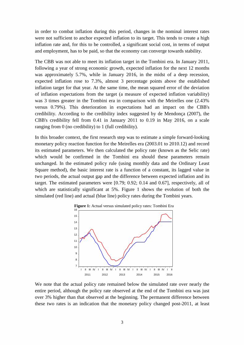
In this broader context, the first research step was to estimate a simple forward-looking
monetary policy reaction function for the Meirelles era (2003.01 to 2010.12) and record
its estimated parameters. We then calculated the policy rate (known as the Selic rate)
which would be confirmed in the Tombini era should these parameters remain
unchanged. In the estimated policy rule (using monthly data and the Ordinary Least
Square method), the basic interest rate is a function of a constant, its lagged value in
two periods, the actual output gap and the difference between expected inflation and its
target. The estimated parameters were [0.79; 0.92; 0.14 and 0.67], respectively, all of
which are statistically significant at 5%. Figure 1 shows the evolution of both the
simulated (red line) and actual (blue line) policy rates during the Tombini years.
Figure 1: Actual versus simulated policy rates: Tombini Era
We note that the actual policy rate remained below the simulated rate over nearly the
entire period, although the policy rate observed at the end of the Tombini era was just
over 3% higher than that observed at the beginning. The permanent difference between
these two rates is an indication that the monetary policy changed post-2011, at least
7
8
9
10
11
12
13
14
15
16
I II III IV I II III IV I II III IV I II III IV I II III IV I II
2011 2012 2013 2014 2015 2016

4
compared to the monetary policy rule over the previous period, and that adverse supply
shocks were not taken into account in either period3.
In fact, when the actual real interest rate was compared to the time-varying long term
equilibrium interest rate4, calculated using the Hodrik-Prescott (HP) filter, we noted that
from the first half of 2012 to the third quarter of 2013 monetary policy remained
expansionist: the actual interest rate was lower than one which, theoretically, could
maintain the output gap at zero and inflation at its target level. Not coincidentally,
official data demonstrates that the expected inflation over these seven quarters ranged
from 5.33% to 5.96%, at a time when the inflation target was 4.5%. On the other hand,
when we compared the expected market inflation twelve months ahead with the ex-post
accumulated inflation rate twelve months later, we saw that, over the entire Tombini
era, the forecast error (expected inflation minus ex-post inflation) remained negative,
while in the Meirelles era this forecast error oscillated between negative and positive
values. This suggests that the dynamic behavior of expected inflation was more
favorable to the central bank under the Tombini chairmanship.
Remaining with our preliminary analysis, we estimated Vector Autoregression (VAR)
models with variables: interest rate, output gap and the gap between expected inflation
and its target. Following estimations and analysis of the main diagnostic tests, the
impulse-response functions were computed for two distinct subsamples: one for the
Meirelles and another for the Tombini era. The generalized impulse-response functions
of the two VAR models, both with two lags, are shown in Figure 2. These are the
interest rate responses over twelve periods due to shocks of one standard deviation
(0.92% in the annualized rate) in the gap between expected inflation and its target.
Figure 2: Generalized impulse-response functions
-.1
.0
.1
.2
.3
.4
.5
1 2 3 4 5 6 7 8 9 10 11 12
Meirelles Era Tombini Era
We note that the interest rate response is only significant at a 95% confidence interval
following the fourth period (in the case of the Meirelles era) and the sixth period (in the
3 In terms of the inflation of monitored prices, we observe that variation in these prices, which are not
sensitive to interest rate movement, only surpassed the accumulated annual inflation mark of 6% in two
periods. The first was in the Meirelles era, from the first half of 2003 to the third quarter of 2006, and the
second was in the Tombini era, from the first quarter of 2015 to the second quarter of 2016. 4 For the real interest rate we used the pre-DI SWAP rate for 360 days discounted from inflation
expectations for the following 12 months. Neither the real interest rate nor the equilibrium real interest
rate are reported here, but are available on request.

5
Tombini one). It is possible to observe that, although the response of the interest rate is
positive in the two subsamples, for most of the simulation horizon, the interest rate
response of the Meirelles era is higher following the third period. Indeed, the
cumulative impact on interest rates in the twelfth period after the expected inflation
shock is 3.3% in the first subsample and 2.6% in the second. This suggests that the
monetary policy was less reactive to deviations in expected inflation during the Tombini
era than in the Meirelles one. These same impulse-response function patterns are
observed when the VAR models are estimated with 3 and 4 lags.
In general, the results of the exercises performed in this section suggest, albeit in a
preliminary manner, that the parameters of the CBB's reaction function changed under
the Alexandre Tombini chairmanship, so that monetary policy became more flexible
and potentially destabilizing. One justification for this change in monetary authority
behavior is a greater concern with economic growth5, which ends up generating more
inflation without the guarantee of better dynamism in the real GDP growth rate over the
medium term. In fact, the average inflation rate during the Tombini era was 0.5% higher
than the same rate during the Meirelles era, which includes the atypical year of 2003.
The average real GDP growth rate, on the other hand, was 3.5% lower. However, the
causal relationship between the flexibility of monetary policy and the depth and
duration of the recession that began in 2014 will not be investigated here.
3. Model specification and database
Based on the contributions of Judd and Rudebusch (1998) and Clarida, Galí and Gertler
(1998), the monetary policy reaction function considered in this study has partial
adjustment and assumes the following format:
tttt
e
tt eehii )]()()[1(. 43
*
212 . (1)
According to this forward-looking specification of the Taylor rule, in addition to a
constant ( 1 ) and its value lagged in two periods ( 2ti ), the interest rate in each period
of time ( ti ) depends on the gap between expected inflation (e ) and the inflation target
(* ), the output gap ( th ) and the percentage change in the real exchange rate in relation
to its long-term trend ( tt ee ). It is assumed that the error term ( t ), which represents
random exogenous shocks in the basic interest rate, is i.i.d, and that the parameter
measuring the degree of interest rate smoothing ( ) is in the interval (0,1).
If we define ,)1(;)1(;)1(;)1( 44332211
5 While it cannot be categorically stated that the CBB was the target of political interference during the
Tombini era, certain statements made by President Dilma Rousseff in South Africa on 03/27/2013 are
symptomatic: "I do not agree with anti-inflation policies that look at the issue of economic growth" (...)
"we do not think that inflation is out of control. On the contrary, we think it is controlled, and there are
changes and conjunctural fluctuations". We note that in March 2013 the inflation accumulated over 12
months exceeded the upper target limit (6.5%), while the expected inflation for the following 12 months
was 5.53%, one percentage point above the central inflation target.

6
the monetary policy reaction function can be rewritten as follows:
tttt
e
tt eehii )()(. 43
*
212 (1’)
i , i = 1, ..., 4 are the short term parameters and i , i = 1, ..., 4 are the long term ones.
It is expected that all the estimated parameters will present a positive signal, since it is
assumed that the monetary authority demonstrates countercyclical behavior and that real
exchange rate devaluations are accommodated through monetary policy. In particular, it
is expected that the parameter )1/(22 will be greater than one. Given an
increase in expected inflation, for instance, the central bank should increase the nominal
interest rate more than proportionately above the increase in expected inflation, so that
the real interest rate will also be affected in the same direction6. When discussing this,
Clarida, Galí and Gertler (2000, p. 152) show that 1)1/(22 and
0)1/(33 are necessary conditions for the forward-looking monetary policy
rule to be stabilizing. These authors point out that, should these conditions not be
confirmed, the monetary policy rule is likely to be destabilizing.
In line with the literature, the lagged interest rate was considered in the monetary policy
rule, in order to capture the stylized fact of the central bank’s smooth adjustments to the
interest rate7. However, unlike the literature consulted for Brazil, the second lag of
interest rate was considered, rather than the first. We proceeded thus because, after
2006, the CBB's Monetary Policy Committee held its meetings to set the interest rate
target every 45 days.
In order to include the exchange rate shock within the model, some authors, such as Ball
(1998), Hausmann, Ugo and Ernesto (2001), Taylor (2002) and Calvo and Reinhart
(2002), argue that in small open economies with a floating exchange rate regime and
subject to external shocks, as is the case of Brazil, exchange rate dynamics should be
carefully monitored. In this case, the monetary authority tends to react to these
exchange rate movements with changes to the nominal interest rate or with international
reserves8. In addition, works that estimate versions of the monetary reaction function for
6 This condition is similar to the well-know "Taylor principle": the proposition that monetary authorities
can stabilize the economy by raising their basic interest rate more than one-for-one in response to higher
inflation. Note that in the context of a simple New Keynesian model, if the condition described above is
not verified, higher expected inflation causes a reduction of the ex-ante real interest rate, which stimulates
demand and generates higher inflation. In this case, the macroeconomic equilibrium becomes
indeterminate and the monetary policy rule does not prevent fluctuations due to self-fulfilling
expectations. Clarida, Gali, and Gertler (2000), for example, argued that the failure of Federal Reserve
policy to satisfy this condition may have been the reason for the macroeconomic instability in the US in
the 1960s and 1970s. 7 For a more in-depth discussion of this topic, see Goodhart (1997) and English, Nelson and Sack (2003).
8 One the one hand, Minella et al (2003, p. 25) included exchange rates in their monetary policy rule and
pointed out that “the central bank may react to exchange rate movements to curb the resulting inflationary
pressures and to reduce the financial impact on dollar denominated assets and liabilities in the balance
sheet of firms”. On the other hand, Taylor (2000) argues that the monetary policy rule in which the
central bank reacts directly to movements in the exchange rate (in addition to inflation and output) does
not work as well in terms of stabilizing inflation and economic activity when compared to a simple rule in

7
the Brazilian economy generally include exchange rate shocks (real or nominal) in some
specifications. In this research, we used monthly data for the period from 2003.01 to
2016.12.
In the light of these considerations, we now move to a description of the variables used
in our empirical analysis. The interest rate (the policy rate) is the nominal Selic rate
accumulated in annual terms and was obtained from the CBB website. This rate is
controlled by the CBB and is the main instrument of monetary policy in Brazil.
Expected inflation over the next twelve months is measured by the median of market
expectation for the accumulated variation in the consumer price index (IPCA), the
official price index for Brazil’s inflation targeting system. This series was obtained from
a survey undertaken by the CBB from a sample of 100 financial market participants and
is available in its “Focus Bulletin”.
The inflation target is the central target for IPCA variation over the current and
following years, defined by the Brazilian National Monetary Council (CMN). The
expression proposed by Minella et all (2003) was used to calculate the gap between
expected inflation and its target level in the years in which the current year’s inflation
target differed from the subsequent year’s one9.
We considered four alternative output gap measures: i) Gap1: the percentage variation
in the seasonally adjusted economic activity index, called the IBC-Br (extracted from
the CBB website), around its potential level, calculated using the HP filter (λ=14.400);
ii) Gap2: the regression residuals between the IBC-Br and the combination of one linear
and one quadratic trend; iii) Gap3: the percentage variation of seasonally adjusted
industrial production, extracted from the Brazilian Institute of Geography and Statistics
(IBGE) around its long-run trend (using the HP filter) and iv) Gap4: variation in the
level of industry capacity utilization (obtained from the Ipeadata website), around its
long-run trend (using the HP filter). For its part, the exchange rate shock is the
percentage change in the real effective exchange rate (obtained from the CBB website)
in relation to its long-run trend (calculated using the HP filter).
The standard model is the one that considers the first output gap proxy. Figure 3
contains the variables used in this specification:
which the central bank only reacts indirectly to exchange rate shocks. The author also points out that, in
the case of developed economies, if the central bank reacts strongly to movements in the exchange rate,
the product performance tends to deteriorate, which was why he decided not to insert the exchange rate in
the rule suggested in his seminal 1993 work. 9 The expression used was the following weighted average: )(
12)(
12
12 *
2_
*
1_ year
e
year
e tt
. Note
that when the inflation target of one year is identical to the inflation target of the next year, this
expression can be simplified as the simple difference between expected inflation and its target.

8
Figure 3: Series used in the standard model
Following the majority of the empirical literature, the forward-looking monetary policy
reaction function was estimated by the Generalized Moment Method (GMM). One of
the justifications for using this, rather than the traditional Ordinary Least Squares
(OLS), method is that the GMM corrects occasional endogeneity problems, thus
avoiding inconsistency in estimated parameters. The expected inflation variable, for
example, is probably endogenous, as Clarida, Galí and Gertler (1998, 2000) and
Gonçalves and Fenolio (2007) have argued. We note that the instruments used in each
estimation must be uncorrelated with the error term. Since the lagged explanatory
variables possess this property, they are immediate instruments. Following this
principle, the interest rate lagged in two periods was used as its own instrument, while
the instruments for the other explanatory variables were their values lagged in one
period. In addition, following the suggestion of Gonçalves and Fenolio (2007), we used,
in our vector of instruments, the first difference of the Pre-DI SWAP rate for 30 days
(this was obtained from the CBB website) and discounted from the country-risk, as
measured by the EMBI+ Brazil (Emerging Markets Bond Index Plus) index of JP
Morgan Bank.
4. Results
Before estimating the parameters of the monetary policy rule, we tried to ascertain
whether the time series used in this study were stationary. This procedure was adopted
in order to avoid obtaining spurious results. The question is whether the interest rate and
the gap between expected inflation and its target level were stationary, since we know
that, by definition, the other series are I(0). The Augmented Dickey-Fuller (ADF) and
the Phillips-Perron (PP) tests were used in the specification with no constant and no
-2
-1
0
1
2
3
4
2004 2006 2008 2010 2012 2014 2016
Expected Inglation Gap
-6
-4
-2
0
2
4
2004 2006 2008 2010 2012 2014 2016
Output Gap (Gap1)
5
10
15
20
25
30
2004 2006 2008 2010 2012 2014 2016
Nominal Interest Rate
-20
-10
0
10
20
30
2004 2006 2008 2010 2012 2014 2016
Exchange Rate Shock

9
trend. The null hypothesis for these two tests is that the series has a unit root against the
alternative of stationarity. The statistics for these tests are shown in Table 1.
Table 1
Variable ADF PP
ti -1.84*** (4) -1.73* (9) * e
-2.90*** (1) -3.08*** (6)
Note: ***denotes significance at 1%, **
at 5%, *
at 10%.
As can be seen, it is possible to reject the unit root null hypothesis for the two series at
the usual levels of significance. Thus, since uncertainty about the stationarity of the
variables has been reduced, the empirical analysis that follows will consider these
variables in level, alongside the output gap and the exchange rate shock measures.
The main results of the econometric estimations are presented in Table 2. All the
estimates are consistent with the presence of heteroskedasticity and serial
autocorrelation in the residuals. We chose White as the estimation weighting matrix in
order to calculate the standard errors.
Table 2: Monetary policy reaction function
Dependent variable: Interest rate
Parameters GMM GMM GMM GMM
β1 -0.06 -0.10 -0.05 0.25
(0.22) (0.25) (0.23) (0.26)
ρ 0.97*** 0.97*** 0.97*** 0.94***
(0.01) (0.02) (0.02) (0.02)
β2 0.36*** 0.39*** 0.32*** 0.47***
(0.03) (0.04) (0.05) (0.06)
β4 0.02** 0.03*** 0.02** -0.01
(0.008) (0.01) (0.01) (0.01)
β3,Gap1 0.29***
(0.03)
β3,Gap2
0.01
(0.01)
β3,Gap3
0.16***
(0.02)
β3,Gap4
0.48***
(0.06)
OBS 166 166 166 166
R² 0.97 0.97 0.97 0.96
Kleibergen-Paap rk LM statistic 62.2*** 50.4*** 48.2*** 49.2***
Hansen J (p-valor) 0.31 0.21 0.26 0.78
Note: ***denotes significance at 1%, **
at 5%, *
at 10%. Standard deviations are in brackets.
First, it should be noted that in all the estimated models the short term coefficients of
the output gap and the difference between expected inflation and the inflation target
were positive, as expected in a central bank that follows an inflation targeting regime.
However, the output gap coefficient calculated from the combination of trends was not
significant. Note that the numerical difference between the estimated parameters
depends on the proxy used for the output gap variable. The smallest short term
coefficient for the expected inflation variable was 0.32, while the highest was 0.47. On

10
the other hand, the statistically significant short term coefficients for output gap ranged
from 0.16 to 0.48.
Taking the standard model into account, the long term expected inflation gap coefficient
was 0.36/(1-0.97)=12, while that for the output gap was 0.29/(1-0.97) )=9.7. We also
noted that in all other estimates the long term expected inflation gap coefficients were
higher than the unit, and the output gap (in three of the four specifications) was
positive10
. In this case, one could say that the CBB's behavior was compatible with
macroeconomic equilibrium during the 2003-2016 period: the CBB reaction function
appeared to be stabilizing.
Second, in the three estimated models, the interest rate coefficient due to real exchange
rate shocks was positive and statistically different from zero. In the specification in
which this parameter was not statistically significant, the sign opposite to that expected
was found. In the standard model, the long term parameter of the exchange rate shock
was smaller than the unit [0.02/(1-0.97)=0.7], probably because movements in the
exchange rate should also affect expected inflation, which is one variable considered in
the model. These results, the small coefficient and significance, were not substantially
different when the real exchange rate shock was replaced by the nominal rate shock in
our estimates (results not reported).
Third, the interest rate smoothing coefficient was statistically significant and high,
floating from 0.94 to 0.97. This result is not surprising, however, since previous studies
which estimated the CBB reaction function using the interest rate level as a dependent
variable [for example Minella et al. (2003), Gonçalves and Fenolio (2007), Sánchez-
Fung (2011) and Medeiros, Portugal and Aragón (2016)] also found high coefficients
for the autoregressive term.
It is important to note that when the model is over-identified it is necessary to test
whether or not the number of instruments over the number of endogenous variables was
expendable. To this end, we performed the Hansen J test, and the null hypothesis of this
test is that all instruments were valid. As can be seen in Table 2, we should not reject
the null hypothesis. On the other hand, two more tests are used in the literature in order
to check whether or not instruments are weak: the Cragg-Donald test and the
Kleibergen-Paap test11
. Statistics from these tests suggested that the instruments we
used were not weak.
In a second step, in order to ascertain whether the behavior of the Brazilian monetary
authority changed during the Alexandre Tombini administration, a multiplicative
dummy variable was added to the model to interact with the variables output gap and
10
In a non-linear specification for the monetary policy rule, examining an open economy and a structural
break in October 2002, Medeiros, Portugal and Aragón (2016) estimated that the long term parameters of
the gap between expected inflation and its target was 8.2, while the output gap was 2.9. 11
In the presence of heteroskedasticity and autocorrelation of residues, the Cragg-Donald statistic is no
longer valid. The Kleibergen-Paap test was therefore used as an alternative.

11
the gap between expected inflation and its target level. The new monetary policy rule
specification assumed the following format:
tt
e
ttt
e
tt hddeehii ])()()()[1(. 16
*
1543
*
212 (2)
in which .)1(;)1( 6655 This new specification can be written as
follows:
.)()()( 16
*
1543
*
212 tt
e
ttt
e
tt hddeehii (2’)
The dummy variable d1 assumed the value 1 for the period from January 2011 to May
2016 (Tombini chairmanship), and zero for the other periods (Meirelles and Goldfajn
chairmanships). If both coefficients that interact with the dummy variable were
statistically significant, we could conclude that the reaction function of the CBB altered
during the Alexandre Tombini chairmanship. If these coefficients were positive
(negative), we could state that the CBB became more rigorous (flexible) in anchoring
expectations and stabilizing economic activity. Using this specification, we can also test
whether the monetary policy became destabilizing. The main results of this new
specification, following model (2'), are summarized in Table 3.
Table 3: Augmented monetary policy reaction function
Dependent variable: Interest rate
Parameters GMM GMM GMM GMM
β1 0.21 0.19 0.21 0.70
(0.25) (0.28) (0.25) (0.27)
ρ 0.95*** 0.95*** 0.95*** 0.91***
(0.02) (0.02) (0.02) (0.02)
β2 0.67*** 0.69*** 0.60*** 0.88***
(0.09) (0.11) (0.11) (0.13)
β4 0.014** 0.03*** 0.02** -0.01
(0.007) (0.01) (0.01) (0.01)
β3,Gap1 0.21***
(0.03)
β3,Gap2
0.02
(0.02)
β3,Gap3
0.11***
(0.02)
β3,Gap4
0.35***
(0.05)
d1*β2 -0.44*** -0.40*** -0.38*** -0.65***
(0.11) (0.12) (0.12) (0.12)
d1*β3,Gap3
0.13***
(0.03)
d1*β3,Gap1 0.11**
(0.05)
d1*β3,Gap4
0.22
(0.14)
d1*β3,Gap2
-0.02
(0.02)
OBS 166 166 166 166
R² 0.97 0.97 0.97 0.97
Kleibergen-Paap rk LM statistic 34.6*** 25.8*** 18.8*** 36.5***
Hansen J (p-valor) 0.11 0.36 0.13 0.32
Note: ***denotes significance at 1%, **
at 5%, *
at 10%. Standard deviations are in brackets.

12
The new estimates suggest that during the Alexandre Tombini era the parameter for
monetary policy rule which relates to the gap between expected inflation and its target is
smaller, since even the coefficient of this variable with no interaction remained positive
and significant, while the interaction parameter of this variable with d1 was negative and
statistically significant at 1% in all estimates (this interaction parameter ranged from
-0.38 to -0.65). On the other hand, the output gap parameter was positive and significant
in three of the four specifications, and its interaction with the dummy variable was only
positive and significant in two. Note also that, according to the standard model with the
dummy variable, the long term parameter related to expected inflation remained greater
than unity (0.67-0.44)/(1-0.95)=4.6 and the output gap parameter remained positive
(0.21+0.11)/(1-0.95)=6.4. Even if we consider the other specifications and the real
exchange rate shock were replaced by the nominal exchange rate shock, it is not
possible to find evidence that the CBB reaction function became destabilizing under
Alexandre Tombini’s chairmanship. Finally, the exchange rate coefficient was positive
and statistically significant in three of the four estimated models (the magnitude of this
coefficient did not change substantially).
The results in Table 3, particularly those relating to CBB behavior due to shocks in
expected inflation and economic activity, are in line with the empirical evidence found
in Curado and Curado (2014) and Barbosa, Camêlo and João (2016). In the former, the
authors suggest that the inflation targeting regime became more flexible during the
Alexandre Tombini era, while in the latter it was not possible to reject the hypothesis
that the CBB changed its reaction function12
from 2011 to 2015. In addition, as noted by
Holland (2005), Soares and Barbosa (2006), Medeiros, Portugal and Aragón (2016) and
Barbosa, Camêlo and João (2016), our study demonstrates that the CBB considered
exchange shocks in its reaction function.
5. Robustness analysis
In this section we re-estimate alternative specifications for the models presented above,
in order to ascertain whether the results described in our standard regression are robust.
To this end, we replaced each actual output gap variable with its lagged value. The other
model variables remained in their original form. The results are shown in Appendix
Table AI, for both the models without the dummy and those where the dummy variable
interacts with the output gap and the gap between expected inflation and its target.
As can be seen, the main results that have been previously found were confirmed here,
although different output gap measures were inserted into the model with one lag. Once
again, the output gap and the exchange rate shock coefficients were not statistically
significant for the specifications that considered the Gap2 variable. On the other hand,
in all the specifications, during the Tombini era, the expected inflation gap coefficient
12
According to the authors' calculation, the long term parameter for the inflation gap decreased from 5.2
in the "Lula period" to 0.4 in the "Dilma period", while the output gap increased from 1.7 to 4.0 during
the "Dilma period".

13
was positive, statistically significant, and smaller. Note that this long term coefficient
remained higher than the unit in all the estimates, including when we used Gap2. It
therefore seems safe to say that CBB behavior was not destabilizing during the recent
period.
6. Concluding Remarks
The evidence found in this paper suggests that, between 2003 and 2016, the CBB’s
reaction function was not destabilizing. On the one hand, we showed that, during the
Alexandre Tombini era, the CBB lent less weight to the gap between expected inflation
and its target, while, at the same time, the interest rate response due to changes in the
output gap was stronger. On the other, no evidence was found to suggest that the
monetary policy rule became incompatible with macroeconomic stability in the
Tombini era. This is in line with the non-explosive behavior of the inflation rate
observed in the post-2011 period. However, changes to the estimated parameters for
monetary policy rule in the Brazilian economy may provide an explanation for the
above-target inflation rates that were consistently observed in the 2011-2016 period, as
well as for the monetary authority’s consequent loss of reputation and credibility under
Tombini’s chairmanship. Finally, the results of this work suggest that the CBB took
exchange rate shocks into account in its reaction function.
References
Aragon, E. K. S. B., Portugal, M. S. (2010). Nonlinearities in Central Bank of Brazil’s
reaction function: the case of asymmetric preferences. Estudos Econômicos. 40 (2),
373–399.
Aragon, E. K. S. B., Medeiros, G. B. (2015). Monetary policy in Brazil: evidence of a
reaction function with time-varying parameters and endogenous regressors. Empirical
Economics, 48(2), p. 557-575.
Ball, L. (1998). Policy Rules for Open Economies. NBER Working Paper 6760.
Cambridge, United States: National Bureau of Economic Research.
Barbosa, F. H; Camêlo, F. D; João, I. C. (2016). A Taxa de juros natural e a regra de
Taylor no Brasil: 2003-2015. Revista Brasileira de Economia, 70(4).
Barcellos Neto, P. C. F. de.; Portugal, M. S. (2007). Determinants of monetary policy
committee decisions: Fraga vs. Meirelles. Porto Alegre: PPGE/UFRGS. (Texto para
Discussão, 11).
Calvo, G., Reinhart, C., (2002). Fear of floating. Quarterly Journal of Economics. 117,
379– 408.
Clarida, R.; Gali, J.; Gertler, M (1998). Monetary policy rules in practice: some
international evidence. European Economic Review, n. 42, p. 1.033-1.067.
___________ (2000). Monetary policy rules and macroeconomic stability: evidence and
some theory. Quarterly Journal of Economics, n. 115, p.147-180.
de Mendonça H. F. (2007). Towards credibility from inflation targeting: the Brazilian
experience. Applied Economics, 39 (19-21): 2599-2615.

14
English, W.; Nelson, W. R.; Sack, B. P. (2003). Interpreting the significance of the
lagged interest rate in estimated monetary policy rules. Contributions in
Macroeconomics 3 (n. 1).
Goodhart, C. (1997), Why Do the Monetary Authorities Smooth Interest Rates? In
European Monetary Policy (S. Collignon, ed.), London: Pinter, 119-174.
Gonçalves, C. E. S., Fenolio, F. R. (2007). Ciclos eleitorais e política monetária:
Evidências para o Brasil. Pesquisa e Planejamento Econômico, 37(3), 465–487.
Hausmann, R., Ugo, P., Ernesto, S., (2001). Why Do Countries Float the Way They
Float? Journal of Development Economics. 66, 387–414.
Holland, M. (2005). Monetary and exchange rate policy in Brazil after inflation
targeting. In XXXIII Encontro Nacional de Economia da ANPEC, Natal, RN.
Judd, J. P., Rudebusch, G. D. (1998). Taylor’s Rule and the Fed: 1970–1997. FRBSF
Economic Review, 3, 3–16.
Mello, L., Moccero, D. (2009). Monetary policy and inflation expectations in Latin
America: long-run effects and volatility spillovers. Journal of Money, Credit and
Banking, 41, 1671-1690.
Medeiros, G. B., Portugal, M. S., Aragón, E. K. (2016). Robust monetary policy,
structural breaks, and nonlinearities in the reaction function of the Central Bank of
Brazil. EconomiA, 17(1), 96-113.
Minella, A., Freitas, P. S., Goldfajn, I., Muinhos, M. K. (2002). Inflation targeting in
Brazil: Lessons and challenges (Working Paper No 53). Brasília, DF: Central Bank of
Brazil.
Moreira, R. R. (2015). Reviewing Taylor rules for Brazil: was there a turning-point?
Journal of Economics and Political Economy, 2(2), 276-289.
Moura, M. L., Carvalho A. de., (2010). What can Taylor rules say about monetary
policy in Latin America? Journal of Macroeconomics. 32, 392–404.
Sánchez-Fung, J. R. (2011). Estimating monetary policy reaction functions for
emerging market economies: the case of Brazil. Economic Modeling, 28, pp. 1730–
1738.
Soares, J. J. S., Barbosa, F. de. H. (2006). Regra de Taylor no Brasil: 1999–2005.
XXXIV Encontro Nacional de Economia, Salvador, BA.
Taylor, J. B. (1993). Discretion versus policy rules in practice. Carnegie-Rochester
Conference Series on Public Policy, 39(1), 195–214.
___________. (2000). Using monetary policy rules in emerging market economies. In
Stabilization and Monetary Policy: The International Experience. Paper presented at
Banco de Mexico’s 75th Anniversary Seminar, Mexico City, November 14–15.
___________. (2001). The role of the exchange rate in monetary policy rules. American
Economic Review, 91(2), 263–267.
Teles, V. K., Brundo, M. (2006). Medidas de política monetária e a função de reação do
Banco Central no Brasil. In XXXIV Encontro Nacional de Economia da ANPEC,
Salvador, BA.

15
Appendix
Table AI: Robustness Analysis
Dependent Variable: Interest Rate
Parameters GMM GMM GMM GMM GMM GMM GMM GMM
β1 0.12 0.36 0.06 0.30 0.10 0.28 0.27 0.71***
(0.20) (0.23) (0.22) (0.25) (0.22) (0.25) (0.24) (0.27)
ρ 0.96*** 0.94*** 0.96*** 0.94*** 0.96*** 0.95*** 0.94*** 0.91***
(0.01) (0.02) (0.02) (0.02) (0.01) (0.02) (0.02) (0.02)
β2 0.30*** 0.61*** 0.35*** 0.63*** 0.27*** 0.51*** 0.45*** 0.85***
(0.04) (0.08) (0.04) (0.01) (0.04) (0.11) (0.06) (0.13)
β4 0.02** 0.02** 0.03*** 0.03*** 0.02*** 0.02*** -0.01 -0.008
(0.008) (0.007) (0.01) (0.01) (0.009) (0.01) (0.01) (0.006)
β3,Gap1(t-1) 0.30*** 0.23***
(0.03) (0.03)
β3,Gap2(t-1)
0.02 0.03
(0.014) (0.02)
β3,Gap3(t-1)
0.17*** 0.12***
(0.02) (0.02)
β3,Gap4(t-1)
0.54*** 0.41***
(0.06) (0.06)
d1*β2
-0.41***
-0.38*** -0.32** -0.64***
(0.10)
(0.11) (0.12) (0.12)
d1*β3,Gap3(t-1)
0.11***
(0.03)
d1*β3,Gap1(t-1)
0.10*
(0.05)
d1*β3,Gap4(t-1)
0.34**
(0.16)
d1*β3,Gap2(t-1)
-0.02
(0.02)
OBS 166 166 166 166 166 166 166 166
R² 0.97 0.97 0.97 0.97 0.97 0.97 0.97 0.97
Kleibergen-Paap rk LM statistic 56.8 44.3 41.3 37.3 50.2 19.4 46.8 48.6
Hansen J (p-valor) 0.64 0.22 0.76 0.53 0.47 0.24 0.76 0.35
Note: ***denotes significance at 1%, **
at 5%, *
at 10%. Standard deviations are in brackets.