HAL Id: hal-00875812https://hal.inria.fr/hal-00875812

Submitted on 24 Oct 2013

HAL is a multi-disciplinary open accessarchive for the deposit and dissemination of sci-entific research documents, whether they are pub-lished or not. The documents may come fromteaching and research institutions in France orabroad, or from public or private research centers.

L’archive ouverte pluridisciplinaire HAL, estdestinée au dépôt et à la diffusion de documentsscientifiques de niveau recherche, publiés ou non,émanant des établissements d’enseignement et derecherche français ou étrangers, des laboratoirespublics ou privés.

Reciprocity identities for quasi-static piezoelectrictransducer models: Application to cavity identificationusing iterated excitations and a topological sensitivity

approachCedric Bellis, Sébastien Imperiale

To cite this version:Cedric Bellis, Sébastien Imperiale. Reciprocity identities for quasi-static piezoelectric transducermodels: Application to cavity identification using iterated excitations and a topological sensitivityapproach. Wave Motion, Elsevier, 2013. hal-00875812

Reciprocity identities for quasi-static piezoelectric transducer

models: Application to cavity identification using iterated excitations

and a topological sensitivity approach

Cédric Bellis, Sébastien Imperiale

Dept of Applied Physics and Applied Mathematics

Columbia University, New York, NY 10027, USA

Abstract

The focus of this article is the transient wave-based detection and identification of defects embedded in isotropic

elastic solids using piezoelectric transducers. This workaddresses this problem within a comprehensive framework

encompassing description of elastic wave propagation within the probed media as well as consideration of the coupling

phenomena induced by the transducers. A fundamental reciprocity identity associated with a quasi-static piezoelec-

tric model is derived to lay the foundations of ensuing developments and approach of this inverse scattering problem.

Modeling of piezoelectric transducers is discussed and application of the proven reciprocity theorem enables the propo-

sition of an iterative construction procedure of electric inputs generating waves expected to focus on the sought defects.

The characteristic features of the inverse problem considered, which uses piezoelectric sensor-based measurements,are

also discussed. Next, the identification problem is investigated by way of an adjoint field-based topological sensitiv-

ity approach that permits the construction of a defect indicator function based on the derived reciprocity identity. For

simplicity of exposition, the studied configurations involve defects in the form of traction-free cavities. Finally, aset

of 2D numerical examples based on the spectral finite-elements method is presented to assess the performances of the

proposed approach in identifying embedded defects from electric measurements.

Keywords. Piezoelectric transducers, Reciprocity identity, Iterated time reversal, Adjoint method, Topological sensi-

tivity.

1 Introduction

Transient elastic or ultrasonic waves are preferred phenomena to probe elastic solids in applications such as non-

destructive material testing [34, 11]. Possible embedded and unknown defects, i.e. localized heterogeneities or geo-

metrical features such as cavities or cracks, are illuminated by waves propagating in the solid body considered while

1

measurements of their scattered counterparts are collected on a subset of the external surface. Based on such boundary

data, a wide range of algorithms aiming at detecting and reconstructing such scattering obstacles have been developed

over the last few decades. For instance, optimization-based approaches are generally concerned with the characteriza-

tion of a finite number of parameters that are quantified by minimization of cost-functionals exploiting the available

data, see e.g. [35, 39]. Alternatively, computationally-efficient techniques centered on the construction and the non-

iterative computation of indicator functions of the soughtdefects have been more recently developed [19, 31, 6]. These

approaches are commonly referred to asqualitative methods[14].

There exists a variety of devices providing full-waveform or partial measurements of boundary displacement fields

based on, e.g., mechanical vibrations or electroactive actuators. In this study, it is assumed that the elastic solids of

interest are probed using ultrasonic piezoelectric transducers. Such transducers are made of piezoelectric materials

which have the property to convert mechanical energy into electric energy, and reciprocally [25]. Here, the piezoelectric

phenomena are investigated within the framework of the quasi-static piezoelectric model [27] which features the elasto-

dynamics equation coupled to Maxwell’s equations reduced to a scalar electric potential constituting the quantity which

can be controlled and recorded during an experiment. In the configuration considered, such a transducer is placed in

contact with the investigated elastic medium and it is used both as the source of the illuminating elastic waves as well

as, as the receiver of the associated echoes [40, 44]. In emission-mode, customized electric potentials are applied on the

active elements of the transducer, which generates a wave propagating in the underlying solid. Alternatively, during the

reception regime, or sensor-mode, electric currents associated with the displacement field generated by the mechanical

waves impinging the sensor are recorded.

In the present study, the defect identification problem is addressed in a comprehensive framework in dimension two

or three, which encompasses description of elastic wave propagation within the probed medium as well as of compan-

ion transient piezoelectric phenomena occurring within the transducer. This approach is based on the recent progress

concerning the mathematical treatment of piezoelectric transducer models in association with the development of a per-

formant and highly accurate simulation tool [27]. Therefore, the fully-coupled problem arising due to the presence of

the piezoelectric transducer is taken into account. Some specific issues arise in this context: Firstly, the presence ofthe

piezoelectric transducer induces an electro-mechanical coupling impacting the elastic field within the probed medium

and thus its observation in comparison with a configuration featuring purely elastic boundary excitation and measure-

ments. Moreover, only time-dependent and discrete scalar measurements of the electric field, rather than full-waveform

data, are accessible. Lastly, in their most general form, the electric measurements are associated with an integral oper-

ator, in time and space, acting on the elastodynamic state associated with the echoes recorded at the sensor’s interface

with the probed medium. In other words, the mapping between boundary elastic field and measured electric potentials

lacks of injectivity and the inverse problem considered is severely ill-posed.

The intended contribution of this work is threefold:

i. Derivation of a time-domainreciprocity identityassociated with the quasi-static piezoelectric model considered,

a terminology which originates from Betti reciprocity theorem [43]. Improving simplified models such as [20, 5] while

2

particularizing the studies [30, 32], this identity, whichcan be seen as stemming from a weak formulation of the problem

or the virtual work principle, corresponds to a cross-relation between Neumann and Dirichlet boundary data associated

with two solution states satisfying the same piezoelectricfield equations over a given geometrical domain. Reciprocity-

based methods are classical techniques in the field of non-destructive testing [1], in particular those based on the so-called

reciprocity gap concept [42, 13]. Therefore, the derived identity constitutes a key result for the proposed approach of

the inverse problem considered and a thread of the ensuing developments.

ii. Application of the reciprocity theorem to a specific model of piezoelectric transducer, i.e. introducing the set

of coupled elastic-electric boundary conditions involvedin the emission and reception regimes. This additional result

provides the framework for the proposition of an iterative procedure aiming at constructing optimal electric excitations

generating elastic waves achieving selective focusing on the unknown defects.

iii. Construction of an indicator function of the sought scattering obstacles which are considered in the form of

traction-free cavities for simplicity of exposition. To that purpose, the chosen approach is based on the concept of topo-

logical sensitivity which revolves around the quantification of the perturbation of a given cost functional induced by

an infinitesimal defect. This method that has been developedand applied in a variety of configurations [19, 12, 16, 6]

is extended to the present context of piezoelectric sensor-based measurements by taking advantages of an adjoint-field

formulation [10] which requires application of the previously derived reciprocity identities.

This article is organized as follows: The elastic-electriccoupled equations describing the behavior of a piezoelectric

solid are presented in Section 2, within the framework of a quasi-static approximation of Maxwell’s equations. The

fundamental result proven in Section 3 is a theorem establishing a reciprocity identity associated with the piezoelectric

model considered in a generic geometrical configuration. Section 4 is concerned with the description of a specific

model of piezoelectric transducer, application of the derived reciprocity identity and construction of optimally-focusing

excitations. Next, the inverse problem considered, i.e. detection and identification of embedded cavities, is stated

in Section 5 and the issues arising when dealing with piezoelectric measurements are discussed. Construction of the

indicator function along the lines of the topological sensitivity approach is presented Section 6. Finally, numerical

results associated with 2D configurations and based on the spectral finite-elements method are shown and discussed in

Section 7.

2 Piezoelectric model

2.1 Preliminaries

LetRd with dimensiond = 2 or 3, be endowed with the euclidean scalar product denoted by

u·v =

d∑

i=1

ui vi ∀(u,v) ∈ Rd × R

d. (1)

3

The spaceL(Rd) of linear mappings fromRd into itself, whose elements are second-order tensors satisfying

(ε·u)i =d

∑

j=1

εijuj ∀ε = (εij) ∈ L(Rd), ∀u ∈ Rd,

is equipped with the scalar product

σ :ε =d

∑

i,j=1

σij εij , ∀(σ, ε) ∈ L(Rd)× L(Rd). (2)

Moreover, letL2(Rd) denote the space of linear mappings fromL(Rd) into itself, in which any element is associated

with a fourth-order tensor such asC = (Cijkl) satisfying

(C :ε)ij =

d∑

k,l=1

Cijkl εkl, ∀(C, ε) ∈ L2(Rd)× L(Rd).

Next, letL(

Rd,L(Rd))

denote the space of linear operators fromRd into L(Rd), i.e. mapping vectors to second-order

tensors. Such operators are associated with third-order tensors such asd = (dkij) satisfying

(d·u)ij =d

∑

k=1

dkij uk.

The transposed tensordT, with respect to the inner products (1) and (2), is an elementof the spaceL(

L(Rd),Rd)

of

linear mappings from second-order tensors to vectors, and it is defined by

(dT :ε)k =

d∑

i,j=1

dkij εij .

The notation div is introduced for the scalar divergence operator which maps vector fields ofRd to real-valued scalars,

together with the vectorial divergencediv mapping the spaceL(Rd) of tensor fields toRd. Let us recall that

(divσ)i = div (σi),

whereσi denotes thei-th line vector ofσ, i.e.σi = σT ·ei with ei an element of a basis ofRd.

To be employed in the ensuing analysis, the Green’s formulaeon a regular enough domainO ⊂ Rd with boundary

∂O, are presented hereafter for the reader’s convenience. Given any symmetric second-order tensorǫ(x), then one has

for (u, v) ∈ H1(O) ×H1(O)

∫

O

div (ǫ·∇u) v dx = −

∫

O

∇u· ǫ ·∇v dx+

∫

∂O

ǫ·∇u·n v dσ,

wheren is the unit outward normal on∂O, and for any symmetric fourth-order tensorC(x) and(u,v) ∈ H1(O)d ×

H1(O)d the following identity holds∫

O

div (C :∇u)·v dx = −

∫

O

∇u :C :∇v dx+

∫

∂O

C :∇u·n·v dσ.

In the two above identities, the integrals along∂O must be understood in the sense of the duality product between

H−1/2(∂O) andH1/2(∂O).

4

2.2 Coupled equations of piezoelectricity

Consider a linear elastic and piezoelectric solidΩD ⊂ Rd, with d = 2, 3, not necessarily bounded and isotropic, to be

composed of two sub-domains, namelyΩT which represents the piezoelectric transducer, andΩDS

the flawed elastic solid

to be investigated. Moreover, letΩS represent the background medium which is supposed to be known whileD ⊂⊂ ΩS

denotes the geometrical open domain occupied by thecompactly containeddefect (or the set thereof) to be identified.

There exists a variety of possible choices depending on the configuration tested, such as cavity, crack, rigid inclusion

or elastic inhomogeneity. As we prefer to keep the presentation simple, the present analysis focuses on traction-free

cavities so that the open domain of interestΩD is defined by

ΩD = ΩT ∪ ΩDS, with ΩD

S= ΩS \D.

Therefore, since dist(D, ∂ΩS) > 0 one has∂ΩT ∩ ∂ΩDS= ∂ΩT ∩ ∂ΩS. As a reference, the open defect-free domain

referred to asΩ is defined by

Ω = ΩT ∪ ΩS,

so thatΩD ⊂ Ω for the configurations considered.

When characterizing the linear elastic behavior of solidΩ, let ρ(x) denote the mass density, which is a strictly,

non-degenerating, positive function, i.e. there exist twopositive scalarsρ− andρ+ such that

0 < ρ− ≤ ρ(x) ≤ ρ+, a.e. x ∈ Ω.

Moreover, the so-called elasticity tensorC(x) ∈ L2(Rd) synthesizes the local elastic material properties at any point x

within the domainΩ, and it has the usual major and minor symmetries

Cijkl = Cklij = Cjikl

The boundedness of the moduli comprisingC together with thermo-mechanical stability conditions also ensure the

existence of two scalarsc− andc+ such that

0 < c−|ε|2 ≤ ε :C(x) :ε ≤ c+|ε|

2, a.e. x ∈ Ω, ∀ ε ∈ L(Rd).

The linearized strain field associated with a displacement fieldu ∈ Rd arising inΩD or Ω, is defined as the symmetric

second-order tensorε[u] ∈ L(Rd) such that

(

ε[u])

ij=

1

2

(

∂uj∂xi

+∂ui∂xj

)

.

In the context of a piezoelectric medium, which is characterized by the ability to convert electric energy into me-

chanical energy, and vice versa, letd(x) ∈ L(

Rd,L(Rd))

stand for the so-called piezoelectric tensor synthesizingthe

corresponding local material properties and which exhibits the following index symmetry

dkij = dkji.

5

In the ensuing analysis, the piezoelectric equations are expressed in terms of the scalar electric potentialϕ, which is

associated with local electric properties that are encapsulated in the second-order permittivity tensorǫ(x) ∈ L(Rd)

defined inRd, which is assumed to be symmetric, i.e.

ǫij = ǫji.

Moreover, owing to the boundedness of these physical parameters and to the reference vacuum permittivity, their exist

two scalarsǫ− andǫ+ such that

0 < ǫ−|ψ|2 ≤ ψ ·ǫ(x)·ψ ≤ ǫ+|ψ|

2, a.e. x ∈ Rd, ∀ ψ ∈ R

d.

It is also assumed that the active piezoelectric elements consist of an open sub-domainΩP ⊂ ΩT of the transducer and,

as a consequence, the piezoelectric tensord vanishes outsideΩP , i.e.

d(x) = 0, a.e. x ∈ Rd \ ΩP . (3)

When the quasi-static approximation of the Maxwell’s equations is valid [25, 27], then the set of coupled piezoelec-

tric field equations inΩ, hereinafter referred to asE(Ω), reduces to

ρ∂2u

∂t2+ αρ

∂u

∂t− div (C :ε[u]) = div (d·∇ϕ), in Ω, t > 0,

E(Ω) :

div(

ǫ·∇ϕ)

= div(

dT :ε[u]

)

, in Rd, t > 0.

(4a)

(4b)

The positive functionα(x) is associated with damping properties of the materials constituting the backing (if any)

of the piezoelectric transducer considered. Note that the term αρ featured in the above equation is introduced for

consistency with a mass-proportional dissipation, see e.g. [29]. Therefore, it is assumed that there exists a positive

scalarα+ such that

0 ≤ α(x) ≤ α+, a.e. x ∈ Ω.

Moreover, both the probed elastic solid and the transducer considered are assumed to be initially at rest, so that the initial

displacement conditions, formally denoted asIu, reads

Iu : u(x, 0) = 0,∂u

∂t(x, 0) = 0, a.e. x ∈ Ω, (5)

while the potential at timet = 0 satisfies

Iφ : ϕ(x, 0) = 0 a.e. x ∈ Rd. (6)

Note that, if homogeneous electric boundary conditions areprovided to complete the problem (4) (see Section 4), then

the conditions (5) are sufficient to ensure the homogeneous initial electric conditionIφ.

Remark 2.1 In the ensuing analysis, the computation of the electric potentialϕ can be reduced to the domainΩP . This

model is mathematically justified in [27] based on the assumption that there exists a high permittivity contrast between

6

the piezoelectric elementsΩP and their surroundings, i.e. providing that the following condition holds

supRd\ΩP

ψ ·ǫ·ψ

inf ΩP ψ ·ǫ·ψ≪ 1, ∀ ψ ∈ R

d.

Therefore, equation(4b) is restricted to the domainΩP .

Next, given the geometrical configuration of the problem considered, theexterior surface reads∂Ω = ∂ΩT ∪ ∂ΩS \

(∂ΩT ∩ ∂ΩS) and it is assumed to be associated with the coupled traction-free boundary condition

Bext :(

C :ε[u] + d·∇ϕ)

·n = 0 on the free-surface∂Ω, (7)

with n being the unit outward normal. The elastic boundary conditions are not complete yet inΩD as no condition has

been specified on the defect boundary∂D. An additional elastic boundary condition denotedBu is defined as

Bu(∂D, t) : C :ε[u]·n = t on∂D, (8)

with t = 0 for the case considered of traction-free cavities.

3 Reciprocity identity

The time convolution[u ⋆ v] at timet ≥ 0 is defined by

[u ⋆ v](x, t) =

∫ t

0

u(x, τ) ⊗ v(x, t− τ)dτ.

for generic time-dependent tensor fieldsu, v. Moreover, the combination of time convolution and single (resp. double)

inner product will be denoted by[u ⋆v] (resp. [u ⋆v]), the operation⋆ (resp. ⋆ ) being thus defined by replacing the

tensor product “⊗” sign by the inner product “·” (resp. “:”) in the above definition.

We are now in a position to present a key result that is paramount in the ensuing analysis as well as in the construction

of a defect indicator function. The following theorem is a reciprocity identity associated with the set (4) of coupled

equations that are reduced to a generic open domainO defined as a subset of the background medium considered and

which also includes the transducer, i.e.

ΩT ⊂ O ⊂ Ω.

Reference to [1] can be made for an overview on reciprocity theorems in elastodynamics, with a particular application

to piezoelectric materials obeying the complete Maxwell’sequations. Note that general reciprocity theorems for piezo-

electric models that take into account thermo-acoustic andmagnetic phenomena are given in [30, 32]. Therefore, the

theorem provided below can be seen as a particularization ofthese results to the piezoelectric model considered, which

is synthesized by field equations (4) and which also includesmaterial damping. To establish this result, care is taken to

describe the featured piezoelectric solutions in the proper functional spaces.

7

Theorem 3.1 Let (u, ϕ) and(u, ϕ) in C1(

[0, Tf ];L2(O)d

)

∩ C0(

[0, Tf ];H1(O)d

)

× C0(

[0, Tf ];H1(ΩP )

)

satisfying,

in a weak sense, the field equationsE(O) for t ∈ [0, Tf ] as well as the initial conditionIu, then these solutions satisfy∫

∂O

(

C :ε[u] + d·∇ϕ)

·n ⋆ u−(

C :ε[u] + d·∇ϕ)

·n ⋆ u

dσ

=

∫

∂ΩP

(

ǫ·∇ϕ− dT :ε[u]

)

·n ⋆ ϕ−(

ǫ·∇ϕ− dT :ε[u]

)

·n ⋆ ϕ

dσ, t ∈ [0, Tf ]. (9)

Proof For simplicity of exposition, a formal derivation of identity (9) is presented based on assumptions of additional

regularity, i.e.

(u, ϕ) and(u, ϕ) in C2(

[0, Tf ];L2(O)d

)

∩ C1(

[0, Tf ];H1(O)d

)

× C1(

[0, Tf ];H1(ΩP )

)

,

while discussion of the interpretation of this relation in the case of minimal regularity is deferred to Remark 3.1.

By taking the convolution and inner product of equation (4a)satisfied by(u, ϕ) with the functionu, then after

integration over the domainO ⊂ Ω one obtains∫

O

(

ρ∂2u

∂t2+ αρ

∂u

∂t− div (C :ε[u])− div (d·∇ϕ)

)

⋆ u dx = 0. (10)

Using the initial conditions (5) and the properties of the convolution product, the time derivatives are shifted tou, i.e.∫

O

(

ρ∂2u

∂t2+ αρ

∂u

∂t

)

⋆ udx =

∫

O

(

ρ∂2u

∂t2+ αρ

∂u

∂t

)

⋆udx. (11)

The regularity assumptions implies that the sumdiv (C :ε[u]) + div (d·∇ϕ) is a square integrable function of space,

although this is not true in general for each term of the sum. Nevertheless, for ease of reading, each of these terms are

formally handled independently in the next equations.

Using the Green’s formula twice, the purely elastic term in (10) is replaced as follows∫

O

div (C :ε[u]) ⋆ u dx =

∫

O

div (C :ε[u]) ⋆udx+

∫

∂O

(C :ε[u]·n ⋆ u− C :ε[u]·n ⋆u) dσ. (12)

Moreover, the electric term is also recast using Green’s formula as∫

O

div (d·∇ϕ) ⋆ udx = −

∫

O

∇ϕ⋆dT :ε[u] dx+

∫

∂O

(d·∇ϕ)·n ⋆ u dσ.

Next, asd(x) = 0 whenx /∈ ΩP and on noting thatΩP ⊂ ΩT ⊂ O, then the volume integral at the right-hand side

of the previous equation can be restricted to the domainΩP . Then, application of Green’s formula in this subdomain,

entails∫

O

div (d·∇ϕ) ⋆ u dx =

∫

ΩP

div (dT :ε[u]) ⋆ ϕdx−

∫

∂ΩP

(

dT :ε[u]

)

·n ⋆ ϕdσ +

∫

∂O

(

d·∇ϕ)

·n ⋆ u dσ. (13)

The intermediate equalities (11–13) are then substituted in (10) and the resulting equation is simplified by noticing that

u is also solution of (4), which leads to∫

O

div (d·∇ϕ) ⋆u dx −

∫

ΩP

div (dT :ε[u]) ⋆ ϕdx =

∫

∂O

(

C :ε[u] + d·∇ϕ)

·n ⋆ u− C :ε[u]·n ⋆u

dσ −

∫

∂ΩP

(

dT :ε[u]

)

·n ⋆ ϕdσ.

8

In a similar fashion, by interchanging the roles ofu, u andϕ, ϕ in (13), the termdiv (d ·∇ϕ) ⋆u can be replaced

accordingly in the previous equation, so that one obtains

∫

ΩP

div (dT :ε[u]) ⋆ ϕ− div (dT :ε[u]) ⋆ ϕ dx =

∫

∂O

(

C :ε[u] + d·∇ϕ)

·n ⋆ u−(

C :ε[u] + d·∇ϕ)

·n ⋆u

dσ+∫

∂ΩP

(dT :ε[u])·n ⋆ ϕ− (dT :ε[u])·n ⋆ ϕ dσ.

The proof is concluded by using equation (4b) for(u, ϕ) and(u, ϕ), which finally yields∫

ΩP

div (dT :ε[u]) ⋆ ϕ− div (dT :ε[u]) ⋆ ϕ dx =

∫

ΩP

div (ǫ·∇ϕ) ⋆ ϕdx− div (ǫ·∇ϕ) ⋆ ϕ dx

=

∫

∂ΩP

(ǫ·∇ϕ·n) ⋆ ϕ− (ǫ·∇ϕ·n) ⋆ ϕ dσ.

Remark 3.1 It may not be clear mathematically whether the integrated boundary terms at the left-hand side of identity

(9), i.e. those involving elastic stresses, exhibit sufficientregularity in time for the convolution products to be defined

properly. However, for solutions having minimal regularity, such as weak solutions, then these terms can be recast as

volume integrals which actual definitions turn out to be rigorous in a functional sense. More precisely, if(u, ϕ) and

(u, ϕ) denote solutions belonging toC1(

[0, Tf ];L2(O)d

)

∩C0(

[0, Tf ];H1(O)d

)

×C0(

[0, Tf ];H1(ΩP )

)

and satisfying,

in a weak sense, the field equationsE(O) for t ∈ [0, Tf ] as well as the initial conditionIu then one has from(4a)

∫

∂O

(

C :ε[u] + d·∇ϕ)

·n ⋆ udσ ≡

∫

O

ρ∂u

∂t⋆

(

∂u

∂t+ αu

)

dx+

∫

O

(C :ε[u] + d·∇ϕ) ⋆ ε[u] dx,

together with the companion equality obtained by interchanging the roles ofu, u and ϕ, ϕ. In the above identity the

right-hand side terms appear to be properly defined, therefore the proven reciprocity relation(9) for such solutions is

valid.

4 Piezoelectric transducer modeling

4.1 Geometry and boundary conditions

In this section, a mathematical model associated with the piezoelectric transducerΩT is presented. As a beginning, the

transducer geometry to be used in the ensuing analysis is specified. The piezoelectric domainΩP ⊂ ΩT is assumed to

be composed of a numberNB of active piezoelectric barsΩiP such that

ΩP =

NB⋃

i=1

ΩiP

with ΩiP∩ Ωj

P = ∅ if i 6= j.

9

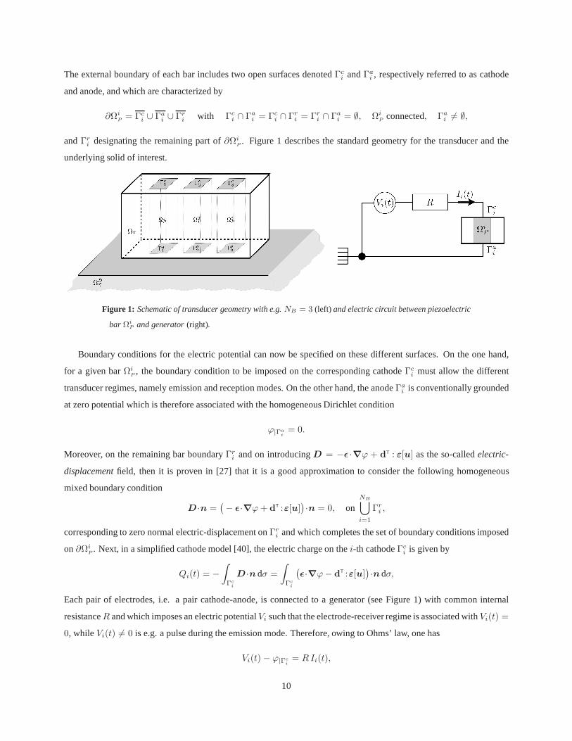
The external boundary of each bar includes two open surfacesdenotedΓci andΓa

i , respectively referred to as cathode

and anode, and which are characterized by

∂ΩiP = Γc

i ∪ Γai ∪ Γr

i with Γci ∩ Γa

i = Γci ∩ Γr

i = Γri ∩ Γa

i = ∅, ΩiP connected, Γa

i 6= ∅,

andΓri designating the remaining part of∂Ωi

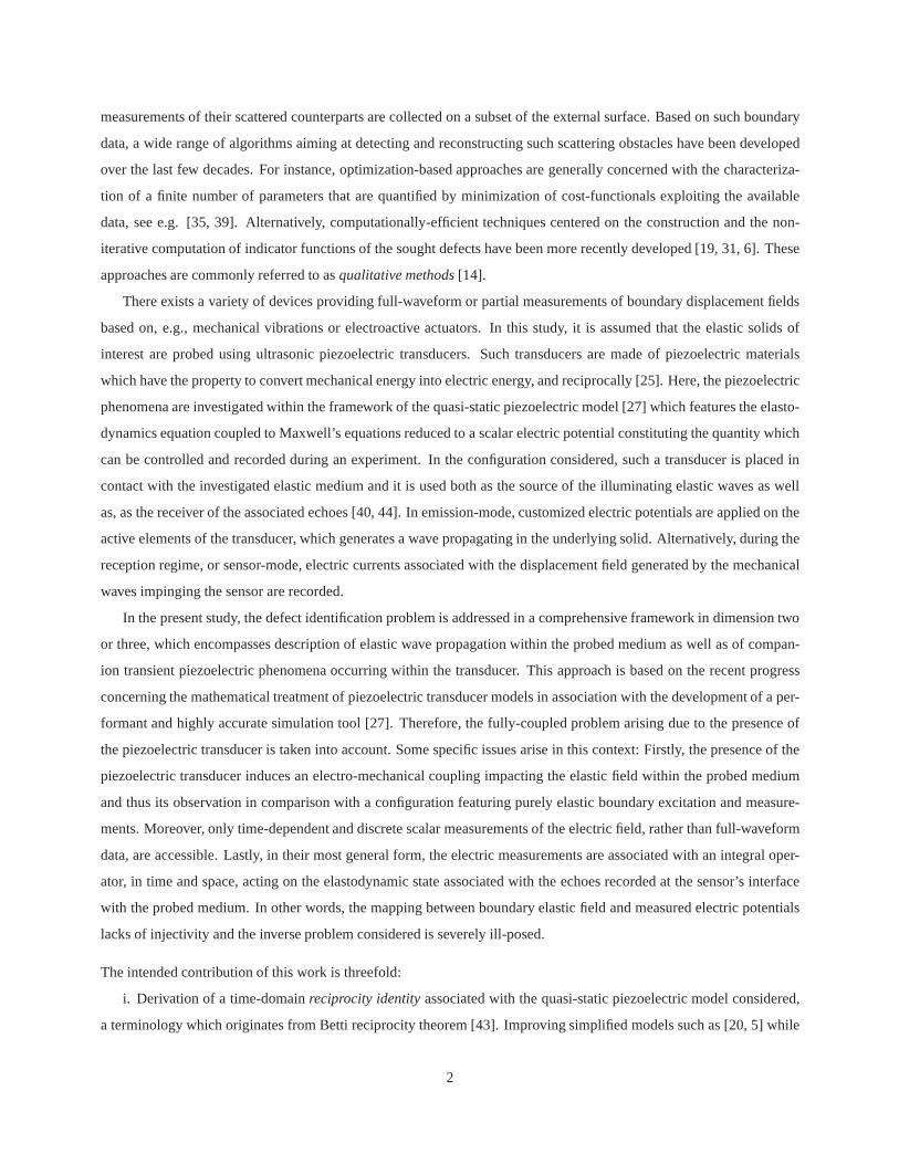
P. Figure 1 describes the standard geometry for the transducer and the

underlying solid of interest.

Figure 1: Schematic of transducer geometry with e.g.NB = 3 (left) and electric circuit between piezoelectric

bar ΩiP and generator(right).

Boundary conditions for the electric potential can now be specified on these different surfaces. On the one hand,

for a given barΩiP

, the boundary condition to be imposed on the corresponding cathodeΓci must allow the different

transducer regimes, namely emission and reception modes. On the other hand, the anodeΓai is conventionally grounded

at zero potential which is therefore associated with the homogeneous Dirichlet condition

ϕ|Γai= 0.

Moreover, on the remaining bar boundaryΓri and on introducingD = −ǫ ·∇ϕ + d

T : ε[u] as the so-calledelectric-

displacementfield, then it is proven in [27] that it is a good approximationto consider the following homogeneous

mixed boundary condition

D ·n =(

− ǫ·∇ϕ+ dT :ε[u]

)

·n = 0, onNB⋃

i=1

Γri ,

corresponding to zero normal electric-displacement onΓri and which completes the set of boundary conditions imposed

on∂ΩiP

. Next, in a simplified cathode model [40], the electric charge on thei-th cathodeΓci is given by

Qi(t) = −

∫

Γci

D ·n dσ =

∫

Γci

(

ǫ·∇ϕ− dT :ε[u]

)

·n dσ,

Each pair of electrodes, i.e. a pair cathode-anode, is connected to a generator (see Figure 1) with common internal

resistanceR and which imposes an electric potentialVi such that the electrode-receiver regime is associated withVi(t) =

0, whileVi(t) 6= 0 is e.g. a pulse during the emission mode. Therefore, owing toOhms’ law, one has

Vi(t)− ϕ|Γci= RIi(t),

10

whereIi(t) is the electric current flowing into the corresponding piezoelectric bar. Since intensity and electric charge

satisfyIi(t) = dQi(t)/dt, then the following mixed boundary condition is finally obtained

ϕ|Γci= Vi(t)−R

d

dt

∫

Γci

(

ǫ·∇ϕ− dT :ε[u]

)

·n dσ.

Then, the coupled electric boundary conditions are synthesized by the following set of equations denoted asBφ:

ϕ = Vi(t)−Rd

dt

∫

Γci

(

ǫ·∇ϕ− dT :ε[u]

)

·n dσ, onΓci , i ∈ 1, . . . , NB, t > 0,

Bφ(Vi) : ϕ = 0, onΓai , i ∈ 1, . . . , NB, t > 0,

(

ǫ·∇ϕ− dT :ε[u]

)

·n = 0, onΓri , i ∈ 1, . . . , NB, t > 0.

(14a)

(14b)

(14c)

For fixed timet, in order to define the electric potentialϕ in the proper functional space, one introduces

W :=

ψ ∈ H1(ΩP ) | ψ = 0 onΓai andψ is constant onΓc

i for i = 1, . . . , NB

.

Therefore, the above space is defined in such way that ifϕ(·, t) ∈ W then the boundary condition (14a) is well defined

whileϕ(·, t) being necessarily constant alongΓci .

Remark 4.1 Consider the complete piezoelectric problem constituted by the field equationsE(Ω), initial conditionsIu

andIφ, as well as boundary conditionsBext, Bu andBφ(Vi) with Vi(t) in L2([0, Tf ])NB . Then this mathematical

problem lies within a classical functional framework whichallows to prove that there exists a unique solution(u, ϕ),

see [27], such that

(u, ϕ) ∈ C1(

[0, Tf ];L2(Ω)d

)

∩ C0(

[0, Tf ];H1(Ω)d

)

× C0(

[0, Tf ];W)

.

4.2 Reciprocity identity involving piezoelectric transducer model

Theorem 3.1 does not specify any particular boundary conditions in terms of displacement or electric potential fields,

therefore identity (9) is satisfied in a generic configurationO ⊃ ΩT when the quasi-static approximation of piezoelec-

tricity holds. The following corollary is a direct application of this theorem when the set (14) of boundary conditions is

introduced. This situation corresponds to the modeling of apiezoelectric transducer in emission and reception modes.

Corollary 4.1 Consider(u, ϕ) and(u, ϕ) inC1(

[0, Tf ];L2(O)d

)

∩C0(

[0, Tf ];H1(O)d

)

× C0(

[0, Tf ];W)

satisfying,

in a weak sense, the field equationsE(O) for t ∈ [0, Tf ], initial conditionsIu andIφ, as well as the electric boundary

conditionsBφ respectively associated with the electric inputsVi(t) andVi(t) in L2([0, Tf ])NB .

Then the following identity holds fort ∈ [0, Tf ]

d

dt

∫

∂O

(

C :ε[u] + d·∇ϕ)

·n ⋆ u−(

C :ε[u] + d·∇ϕ)

·n ⋆ u

dσ =1

R

NB∑

i=1

(

ϕ|Γci⋆ Vi − ϕ|Γc

i⋆ Vi

)

. (15)

11

Proof The starting point to prove this corollary is equation (9). The time derivative of the right hand side of (9) is recast

as

I(t) :=d

dt

∫

∂ΩP

(

ǫ·∇ϕ− dT :ε[u]

)

·n ⋆ ϕ−(

ǫ·∇ϕ− dT :ε[u]

)

·n ⋆ ϕ

dσ

=d

dt

NB∑

i=1

∫

Γci

(

ǫ·∇ϕ− dT :ε[u]

)

·n ⋆ ϕ−(

ǫ·∇ϕ− dT :ε[u]

)

·n ⋆ ϕ

dσ,

where the homogeneous conditions (14b) and (14c) have been used to get rid of the terms respectively integrated over

Γai andΓr

i . On noting that, by definition of the spaceW ,ϕ(·, t) andϕ(·, t) are constant along eachΓci so that they can be

removed from the integral overΓci , and using the property of the convolution product with respect to the differentiation

when homogeneous initial condition such asIφ holds, one finds

I(t) =NB∑

i=1

ϕ ⋆d

dt

∫

Γci

(

ǫ·∇ϕ− dT :ε[u]

)

·ndσ −NB∑

i=1

ϕ ⋆d

dt

∫

Γci

(

ǫ·∇ϕ− dT :ε[u]

)

·n dσ.

This equation is finally simplified using boundary conditions (14a) which finishes the proof.

4.3 Optimally-focusing excitation

To probe the flawed solidΩDS

it is convenient to optimize the illumination generated by the piezoelectric transducer so

that focusing is achieved over a region of interest. The energy of the interrogating elastic wave is thus maximized at a

prescribed location in order to enhance the signal-to-noise ratio associated with this sampling point. Given the geometry

of the transducerΩT considered, then the electric inputsVi(t) applied on the different piezoelectric bars can feature

time-delay parametersτi chosen so as to obtain focusing at the desired location (see,e.g., [26, 27]). Despite its

apparent simplicity, this process relies strongly on the knowledge of the material properties of the transducer and of

the underlying medium. Moreover, the focusing points, withassociated parametersτi, are chosen a priori, which

generally imposes to sample a large region to obtain reliable results. To circumvent these limitations, the proposed

approach aims at optimizing the excitation to achieve focusing on the sought defect(s)D but without having recourse

to any user-chosen parameters. This method finds its roots inthe iterative time reversal approach of acoustic fields and

the decomposition of the so-called time reversal operator which eigenvectors are associated with waves focusing on the

scatterers [36, 38, 37, 24].

Consider the propagation operator for the flawed domain defined as

PD : Vi ∈ L2([0, Tf ])NB −→ ϕ|Γc

i ∈ C0([0, Tf ])

NB

such that(u, ϕ) satisfiesE(ΩD), Iu, Iφ, Bext, Bu andBφ(Vi),

with its defect-free counterpartP associated with the problemE(Ω) in the background domain for which the boundary

conditionBu does not hold. As the solution potentialϕ satisfies the following estimates [27]

NB∑

i=1

‖ϕ|Γci‖2L2([0,Tf ])

≤ T

NB∑

i=1

sup(0,Tf )

(ϕ|Γci)2 ≤ T cp

NB∑

i=1

‖Vi‖2L2([0,Tf ])

. (16)

12

wherecp > 0, thenPD andP are linear and continuous operators. Next, one introduces the smoothing operator

S : ψi ∈ L2([0, Tf ])NB −→ s ⋆ ψi ∈ H1([0, Tf ])

NB ,

where the symbols is a positive causal time-domain function which Fourier transforms satisfies

‖(1 + ω2)1/2s(ω)‖L∞(R) = cs < +∞, (17)

with cs > 0, which implies, based on Fourier transform properties and Parseval’s identity,

NB∑

i=1

‖s ⋆ ψi‖2H1([0,Tf ])

≤ cs

NB∑

i=1

‖ψi‖2L2([0,Tf ])

. (18)

Finally we introduce the time reversal operator

R : ψi(·) ∈ C0([0, Tf ])NB −→ ψi(Tf − ·) ∈ C0([0, Tf ])

NB .

Consequently, we consider the composite operatorH := [RS (PD−P)] which maps electric inputs to the time-reversed

counterpart of the regularized potential residual associated with the perturbation induced by the obstacle D (or the set

thereof). Therefore, it is expected that the eigenfunctions of H that are associated with the eigenvalues of largest

amplitude, if they exist, correspond to excitations generating waves that focus on the sought defect(s). A statement

motived by studies [36, 37, 24]. The operator main property is thus characterized by the following theorem which relies

strongly on Corollary 4.1 and thus on Theorem 3.1.

Theorem 4.1 The linear operatorH = [RS (PD − P)] : Vi ∈ L2([0, Tf ])NB −→ ψi ∈ L2([0, Tf ])

NB xadmits a

countable orthonormal basis of eigenvectors associated with real eigenvalues accumulating at zero.

Proof One has to prove thatH is (i) self-adjoint and (ii) compact. First one proves (i), i.e.H is self-adjoint with respect

to theL2 inner-product in[0, Tf ] that is defined by

(

ψi, Vi)

L2([0,Tf ])NB

=

NB∑

i=1

∫ Tf

0

ψi(t) Vi(t)dt.

On notingPD(Vi) = ϕDi andP(Vi) = ϕi as well asPD(Vi) = ϕDi andP(Vi) = ϕi, then one has

(

H(Vi), Vi)

L2([0,Tf ])NB

=

NB∑

i=1

∫ Tf

0

[s ⋆ (ϕDi − ϕi)](Tf − t) Vi(t)dt

=

[

s ⋆(

NB∑

i=1

(ϕDi − ϕi) ⋆ Vi

)

]

(Tf)

based on the definition of the time reversal operator, the properties of the convolution product and the fact thatϕi are

compactly supported and causal functions. Next, owing to definition of operatorP and Corollary 4.1 with the domain

O coinciding with the background geometry, i.e.O = Ω, one has

NB∑

i=1

ϕi ⋆ Vi =

NB∑

i=1

ϕi ⋆ Vi,

13

using (7). Similarly, definition ofPD together with the piezoelectric reciprocity identity for the configurationO = ΩD

based on (7) and (8) yield

NB∑

i=1

ϕDi ⋆ Vi =

NB∑

i=1

ϕDi ⋆ Vi −Rd

dt

∫

∂D

C :ε[uD]·n ⋆ uD − C :ε[uD]·n ⋆ uD dσ.

whereuD anduD are the displacement field solutions of the complete piezoelectric problem inΩD, respectively associ-

ated with the potentialsϕDi andϕDi on the electrodes. Owing to (8), i.e. the boundary conditionBu imposed on

the defect boundary, then the integral along∂D vanishes in the right-hand side of the previous equation andone finally

obtains(

H(Vi), Vi)

L2([0,Tf ])NB

=

[

s ⋆(

NB∑

i=1

(ϕDi − ϕi) ⋆ Vi

)

]

(Tf)

=

NB∑

i=1

[

Vi ⋆ [s ⋆ (ϕDi − ϕi)]]

(Tf )

=(

Vi,H(Vi))

L2([0,Tf ])NB

,

which proves the self-adjointness of the operatorH.

Then one proves (ii), i.e. thatH is a compact operator. LetVin be a bounded sequence inL2([0, Tf ])NB with

ψin = H(Vin), then as a consequence of estimates (16) and (18) one has

‖ψin‖2H1([0,Tf ])NB

≤ T cp cs‖Vin‖2L2([0,Tf ])NB

, ∀n > 1.

Therefore, the sequenceψin is bounded inH1([0, Tf ])NB so that by Rellich theorem there exists a subsequence that

converges inL2([0, Tf ])NB which, by definition, induces the compactness of the operator H.

The proof is concluded by invoking the spectral theorem.

Construction of optimal excitations. Owing to Theorem 4.1, the operator[RS (PD−P)] admits a countable set of or-

thonormal eigenvectors. Yet, the interpretation of these eigenfunctions are beyond the scope of this study, nonetheless it

is expected that the eigenvalues of largest amplitude are associated with eigenfunctions corresponding to waves radiated

by the different scatterers present within the probed medium [36, 37, 24]. Therefore, one can iteratively define electric

inputs so that the emitted wave will converge to the eigenfunction associated with the eigenvalue of largest amplitude

(in the case where its multiplicity is one), and thus targetsthe strongest scattering obstacleD to be identified.

– LetVi0 ∈ L2([0, Tf ])NB denote the initial input

– ComputeWin = [RS (PD − P)](Vin)

– DefineVin = Win/‖Win‖L∞([0,Tf ])

(19)

Discussion and assessment of this approach capabilities are deferred to Section 7. Note that this power iteration method

can be advantageously superseded by Lanczos iterations [33]. This extension is however left for future work.

14

Remark 4.2 The purpose of introducing the smoothing operatorS is twofold: i) From a theoretical standpoint to en-

force the compactness of the operatorH and thus the convergence of the above algorithm, and ii) froma practical point

of view, to damp the highest frequency phenomena occurring during an experiment or a simulation which could therefore

pollute the proposed iterated procedure. In practice, the smoothing functions(t) is chosen as a causal approximation

of the Dirac delta functionδ(t).

5 Measurements and inverse problem

5.1 Definition

The inverse problem considered consists in detecting the unknown defectD and determining qualitatively its topology

and geometry. To do so, the domainΩDS

is illuminated using a given set of source functionsVi ∈ L2([0, Tf ])NB im-

posed on the piezoelectric transducer’s cathodes. The resultant interrogating electro-mechanical field(uobs, ϕobs), to be

measured, is the solution of the complete piezoelectric problem described byE(ΩD), Iu, Iφ, Bext, Bu(∂D,0) andBφ(Vi),

i.e. equations (4–8) and (14), and one has

(uobs, ϕobs) ∈ C1(

[0, Tf ];L2(ΩD)

d)

∩ C0(

[0, Tf ];H1(ΩD)

d)

× C0(

[0, Tf ];W)

.

To handle the inverse scattering problem considered, it is considered that the only available measurements are the electric

potentials on theNB cathodes of the transducer, therefore the defectD has to be characterized from knowledge of

ϕobs|Γc

i

NB

i=1∈ C0([0, Tf ])

NB . (20)

5.2 Measurements and ill-posedness

Given the nature of measurements (20), a first question concerns the possibility of reconstructing the displacement field

uobs on ∂ΩT ∩ ∂ΩDS . Answering positively this question would ensure the straightforward applicability of existing

inversion strategies, in particular of a class of so-calledqualitative(or sampling) methods using such remote elasto-

dynamic measurements, see e.g. [4, 31, 15, 12] and the references therein. To address this question, the idea is to

establish an explicit relation betweenuobs|∂ΩT∩∂ΩD

Sand the measured potentialϕobs

|Γcℓ

on a given electrodeΓcℓ with

ℓ ∈ 1, . . . , NB.

Let(

Gℓ(x, t),Φℓ(x, t))

denote the fundamental piezoelectric solution associatedwith the electrodeΓcℓ, defined as

the solution of the problemE(ΩT ), i.e.

ρ∂2Gℓ

∂t2+ αρ

∂Gℓ

∂t− div (C :ε[Gℓ]) = div (d·∇Φℓ), in ΩT , t > 0,

div(

ǫ·∇Φℓ

)

= div(

dT :ε[Gℓ]

)

, in ΩP , t > 0,

15

together with electric boundary conditionsBφ(Vi) with sourceVi(t) = δiℓ δ(t)

Φℓ = δiℓ δ(t)−Rd

dt

∫

Γci

(

ǫ·∇Φℓ − dT :ε[Gℓ]

)

·ndσ, onΓci , i ∈ 1, . . . , NB, t > 0,

Φℓ = 0, onΓai , i ∈ 1, . . . , NB, t > 0,

(

ǫ·∇Φℓ − dT :ε[Gℓ]

)

·n = 0, onΓri , i ∈ 1, . . . , NB, t > 0,

which corresponds to the situation where theℓ-th electrode has been excited by an electric Dirac delta function. To

define completely(

Gℓ(x, t),Φℓ(x, t))

the following mixed elastic boundary conditions are added:

(

C :ε[Gℓ] + d·∇Φℓ

)

·n = 0 on∂ΩT \(

∂ΩT ∩ ∂ΩS

)

and Gℓ = 0 on∂ΩT ∩ ∂ΩS,

which are conditions satisfied at the transducer boundary, together with homogeneous initial conditionsIu andIφ. Note

again that in the configuration of interest which involves aninternal defect, one has∂ΩT ∩ ∂ΩDS= ∂ΩT ∩ ∂ΩS.

Remark 5.1 The fundamental piezoelectric solution considered can be interpreted as the limit solution obtained using

parametrized and uniformly bounded source termsVi(t, η) ∈ L1([0, Tf ]) with Vi(t, η) → δiℓ δ(t) whenη → 0.

Existence and uniqueness results can be shown, and one has that the solution(

Gℓ(x, t),Φℓ(x, t))

can be used to

define double-layer potential representations of the piezoelectric solutions. Now, applying, formally, Corollary 4.1 to(

Gℓ(x, t),Φℓ(x, t))

and(uobs, ϕobs) in O = ΩT leads to

ϕobs|Γc

ℓ=

NB∑

i=1

Φℓ|Γci⋆ Vi + R

d

dt

∫

∂ΩT ∩∂ΩS

(

C :ε[Gℓ] + d·∇Φℓ

)

·n ⋆uobsdσ, (21)

which characterizes the measured electric potential at theelectrodeℓ ∈ 1, . . . , NB as a double-layer potential having

the displacement fielduobs on∂ΩT ∩ ∂ΩS as its density.

The measurements (20) considered, consist of a number ofNB time-dependent scalar functionsϕobs onΓcℓ corre-

sponding to a time-dependent spatial average of the three-dimensional vector fielduobs at the interface∂ΩT ∩ ∂ΩDS

between the probed domain and the sensor. Therefore, the displacementuobs|∂ΩT∩∂ΩD

Son the observation surface can-

not be reconstructed uniquely from the knowledge of the electric potentialϕobs on all the electrodes. For example, the

measurements are invariant with respect to the geometricalsymmetries of the sensor considered (classically a cylinder).

More precisely, on using previous representation (21), ascertaining whether or not the mapping between elastic field and

measurements is injective reduces to characterizing the null-space of the integral operatorK defined by

K : u ∈ C0(

[0, Tf ], H1/2(∂ΩT ∩ ∂ΩS)

d)

−→ Ku ∈ C0([0, Tf ])NB

such that(Ku)ℓ =∫

∂ΩT∩∂ΩS

(

C :ε[Gℓ] + d·∇Φℓ

)

·n ⋆u dσ, ℓ ∈ 1, . . . , NB,

whereu is solution of the fully coupled piezoelectric problem.

One can conclude that the measurements (20) at hand in the problem considered are markedly poor in terms of avail-

able informations for the following reasons: i) The use of the piezoelectric transducer induces an electro-mechanical

16

coupling which impacts the observation of the field scattered by the sought obstacleD compared to a configuration em-

ploying purely elastic boundary conditions and excitation. ii) The measurements involve remote boundary observations

on ∂ΩDS

and spatial averaging of the probing elastodynamic stateuobs arising inΩDS⊂ ΩD. iii) Only time-dependent

scalar, rather than vectorial, quantities are available. To circumvent these limitations, the approach proposed in [8] con-

sists in considering the identification problem within the limit geometric configuration of a slender piezoelectric bar, for

which an explicit relation between the measured electric potential and the elastic displacement field at∂ΩT ∩ ∂ΩS can

be established by asymptotic analysis.

6 Topological sensitivity approach

This section concerns the construction of a defect indicator function based on the concept of topological sensitivity and

on an adjoint-field based approach that uses the derived reciprocity identity (15) of Corollary 4.1.

6.1 Presentation

Identification of the defectD is based on the availability of electric potential measurements of the form (20) during

the time interval[0, Tf ] and corresponding to a coupled probing elastodynamic-electric state(uobs, ϕobs) arising in the

flawed solid and the transducer due to electric excitation prescribed on the electrodes. The discrepancy between a

trial configurationΩ∗D

and the unknown domainΩD is evaluated by means of a cost functionalJ in terms of a given

misfit density function. Such a misfit function is chosen so asto evaluate the gap between observationsϕobs|Γc

iand

measurementsϕ∗|Γc

iof the potential solution associated with the trial flawed solid Ω∗

D. Numerical experiments presented

in this work are based on a commonly-used least squares misfitfunction, i.e.

J(ϕ∗;Tf) =1

2

∫ Tf

0

NB∑

i=1

∣

∣ϕ∗|Γc

i− ϕobs

|Γci

∣

∣

2dt, (23)

where the experiment durationTf appears as an adjustable parameter.

The topological sensitivity of the cost functional (23) is here defined as its sensitivity with respect to the creation

of an infinitesimaltraction-free obstacleof characteristic sizea at a given locationz ∈ ΩS and formally defined by

Da,z = z + aD in terms of a characteristic radiusa > 0 and a normalized open surfaceD containing the origin and

specifying a chosen shape (e.g.D is a unit sphere for a nucleating spherical cavity inR3). The corresponding trial open

flawed domain is defined such that

Ω∗D:= Ωa,z = ΩT ∪ (ΩS \Da,z).

In Ωa,z, the prescribed electric excitation gives rise to a coupledstate(ua,z, ϕa,z) that can be conveniently decomposed

by linearity intoua,z = u|Ωa,z+ va,z andϕa,z = ϕ|Ωa,z

+ψa,z, where the free-field solution(u, ϕ) is the response of

the referencedefect-freedomainΩ, i.e.

(u, ϕ) satisfies E(Ω), Iu, Iφ, Bext andBφ(Vi), (24)

17

while (va,z, ψa,z) denotes the perturbation induced by the nucleating infinitesimal obstacle, such that

(va,z, ψa,z) solves E(Ωa,z), Iu, Iφ, Bext, Bφ(0) andBu(∂Da,z,−C :ε[u]·n). (25)

Following earlier works on topological sensitivity, e.g. [45, 21, 12], one seeks the asymptotic behavior ofJ(ϕa,z;Tf)

asa → 0 through an expansion of the cost functional (23) about(ua,z, ϕa,z) = (u|Ωa,z, ϕ|Ωa,z

) to first order w.r.t.

(va,z, ψa,z) = (ua,z − u|Ωa,z, ϕa,z − ϕ|Ωa,z

), i.e.

J(ϕa,z;Tf ) =a→0

J(ϕ;Tf) + [J′(ϕ;Tf )](ψa,z) + o(

‖ψa,z‖)

(26)

wherelima→0 ‖ψa,z‖ = 0 andJ′ is the derivative ofJ in the direction of the field perturbation.

Owing to first-order Taylor expansion of the misfit function,one has

[J′(ϕ ;Tf )](ψa,z) =

∫ Tf

0

NB∑

i=1

(

ϕ− ϕobs)

|Γci

ψa,z |Γci

dt. (27)

Evaluating (27) is done by quantifying the leading asymptotic behavior in asymptotics (26) asa→ 0. One possible way,

along the lines of the so-called direct differentiation approach of parameter or shape sensitivity analysis [23], consists

in seeking the asymptotic behavior ofψa,z onΓci for i ∈ 1, . . . , NB and plugging the result into (27). As previously

discussed on several occasions [10, 6], however, a more compact formulation for actual evaluation of[J′(ϕ|Ωa,z)](ψa,z)

can be set up using an adjoint-field based approach and is adopted here.

6.2 Piezoelectric sensor model

6.2.1 Adjoint-field formulation

The key idea of the adjoint formulation stems from treating the integral in the right-hand side of (27) as one of the terms

arising in the reciprocity identity (15) linking two piezoelectric states, in which one state is the perturbation(va,z, ψa,z)

while the other is chosen as a so-called adjoint solution(u, ϕ) to be defined appropriately.

Consider the electric inputsVi defined by the time-reversed counterpart of the measurements residuals, i.e.

Vi(t) =(

ϕ− ϕobs)

|Γci

(Tf − t) for i ∈ 1, . . . , NB, t ∈ [0, Tf ], (28)

and let(u, ϕ) be a piezoelectric solution in the reference defect-free domainΩ of the following problem

(u, ϕ) solves E(Ω), Iu, Iφ, Bext andBφ(Vi). (29)

Now, on applying Corollary 4.1 to the solutions(u, ϕ) and(va,z, ψa,z) in the subdomainO = Ωa,z and owing to the

corresponding initial conditions and applied excitationsin (25, 29), then equation (15) is recast in

Rd

dt

∫

∂Ωa,z

(

C :ε[u] + d·∇ϕ)

·n ⋆ va,z −(

C :ε[va,z] + d·∇ψa,z

)

·n ⋆ u

dσ =

NB∑

i=1

Vi ⋆ ψa,z |Γci. (30)

18

On using definition (28), then the right-hand sides of the equations (27) and (30) turn out to be equal, therefore, and

owing to hypothesis (3) and the relevant boundary conditions in (25, 29) on the infinitesimal defect boundary∂Da,z as

well as on the exterior surface∂Ωa,z \ ∂Da,z, the derivativeJ′ reduces to

[J′(ϕ ;Tf )](ψa,z) =

NB∑

i=1

Vi ⋆ ψa,z |Γci= R

d

dt

∫

∂Da,z

C :ε[u]·n ⋆ u+ C :ε[u]·n ⋆va,z dσ. (31)

6.2.2 Topological derivative

Next, the so-calledtopological derivativefunctionT can be defined through the identity

[J′(ϕ ;Tf)](ψa,z) =a→0

η(a)T(z ;D, Tf ) + o(η(a)),

where the functionη(a) vanishing in the limita → 0. The coupled piezoelectric state(va,z, ψa,z) exhibits an asymp-

totical behavior, however, as emphasized in the equation (31), one is only interested in the leading contribution ofva,z

on ∂Da,z asa → 0. Since the sampling pointz varies within the elastic domainΩS, i.e. not within the piezoelectric

material domainΩT , then in the limita → 0 the coupled boundary condition at the transducer interface∂ΩT ∩ ∂ΩS

does not enter the asymptotics ofva,z. Consequently, the expressions established by local analysis for purely elastic

configurations in, e.g., [45, 21, 22, 3], remain valid in the present situation and hence, the right-hand side of equation

(31) can now be computed by inserting the appropriate asymptotic behavior ofva,z, see details provided in Section 3 of

[6]. Finally, with the second-order stress tensor defined asσ[v] = C :ε[v] in L(Rd) and the symbol⋆ denoting a time

convolution involving the inner product (2), one obtains

η(a) = ad|D|, (32a)

T(z ;D, Tf) = Rd

dt

(

σ[u] ⋆A(D) :σ[u] + βdu

dt⋆du

dt

)

(z), (32b)

where the so-calledelastic moment tensorA ∈ L2(Rd) depends on the shape of the infinitesimal traction-free obstacle

Da,z that is featured in the asymptotic analysis, while regardless of this cavity shapeβ = ρ (see, e.g., [22]).

The computation of the indicator functionT requires the knowledge of the free-fieldu and the adjoint-fieldu re-

spectively defined by the problems (24) and (29) in the reference defect-free domainΩ. Moreover, the parameterA

entering the definition (32b) can be computed for any arbitrary shapeD by solving canonical elastostatic exterior prob-

lems [22]. However, it can be found in a closed form when the assumed obstacle shapeD in relatively simple, e.g.D

being a sphere inR3. Such a closed form is preferred for the purposes of the present study, and the formula established

in previous studies are listed hereafter for the reader’s convenience.

Consider the case whereΩS is a homogeneous linear elastic and isotropic solid characterized by shear modulusµ

and Poisson’s ratioν, so that the elasticity tensor reduces to

C = 2µ

[

Isym+

ν

1− 2νI ⊗ I

]

19

whereIsym andI denote respectively the symmetric fourth-order and second-order identity tensors. Then, for the

configurations addressed in this study, the material parameters in (32b) reduce to the following expressions depending

on the chosen shapeD: For the case of a spherical (resp. circular) cavity nucleating in the 3D (resp. 2D) elastic body

considered, one has|D| = 4π/3 (3D) or |D| = π (2D) and from [21]

A =3(1− ν)

2µ(7− ν)

[

5Isym−1 + 5ν

2(1 + ν)I ⊗ I

]

(3D) (33a)

A =1− ν

µ

[

2Isym−1

2(1 + ν)I ⊗ I

]

(2D plane strain) (33b)

Remark 6.1 Note that the previous developments are not intrinsically limited to a choice of elastic boundary conditions

such as(8) and the proposed approach can be easily generalized to the case of inhomogeneous elastic scatterers. In

such a case, the parametersA andβ depend additionally on the assumed elastic parameters of the infinitesimal trial

obstacle. In the case of a small nucleating spherical elastic inclusion, closed-form expressions can be found in [16].

Further generalizations of the topological sensitivity approach include the case of traction-free cracks [7]

7 Numerical results

7.1 Implementation

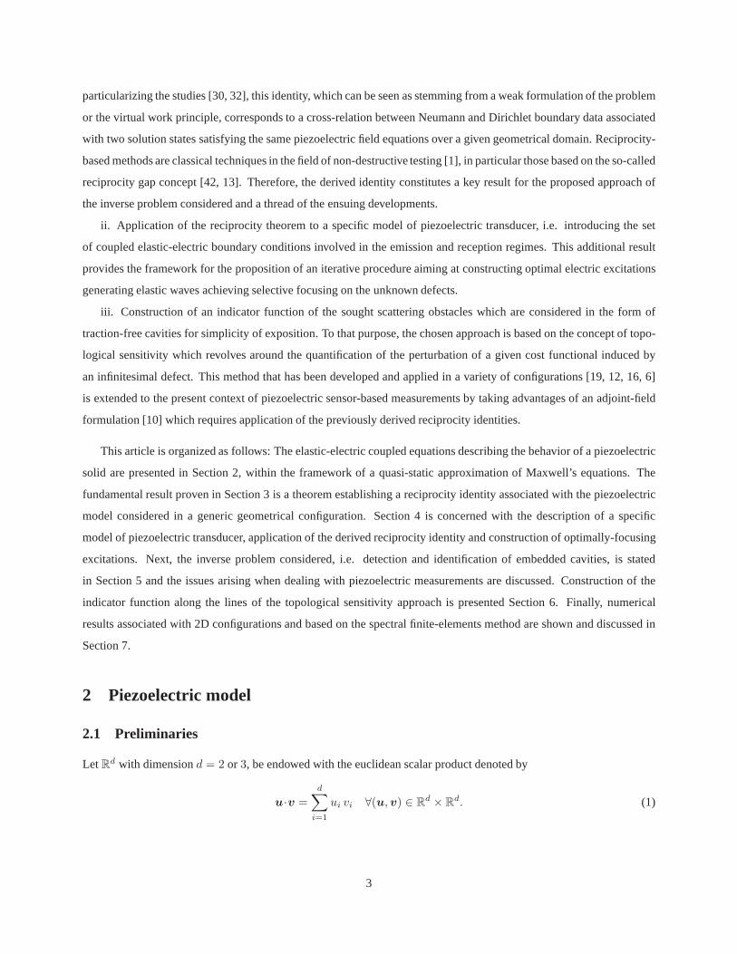
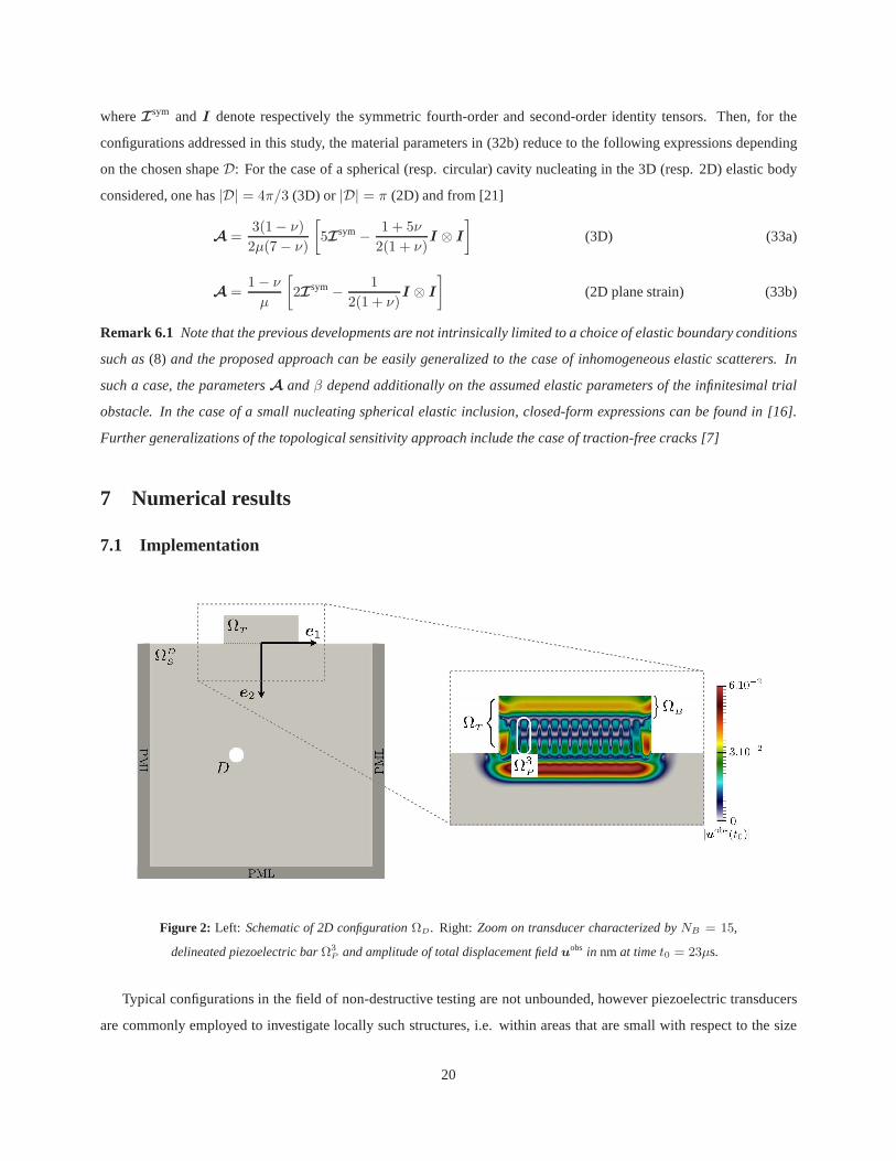
Figure 2: Left: Schematic of 2D configurationΩD. Right: Zoom on transducer characterized byNB = 15,

delineated piezoelectric barΩ3

P and amplitude of total displacement fielduobs in nm at timet0 = 23µs.

Typical configurations in the field of non-destructive testing are not unbounded, however piezoelectric transducers

are commonly employed to investigate locally such structures, i.e. within areas that are small with respect to the size

20

of the overall body which can then be seen as unbounded at the scale considered. Therefore, the numerical experiments

presented hereafter correspond to the probing of a two-dimensional and homogeneous half-spaceΩDS . An example ge-

ometry of a studied configuration is described Figure 2 with width and height corresponding respectively to dimensions

along axese1 ande2: The transducer of widthl = 30mm is composed ofNB equidistributed bars of widthl/2NB and

height6.3mm. A 5mm-height dissipative backing denotedΩB lies atop the domainΩP , so that the dissipation parameter

α in equation (4) is characterized bysuppα = ΩB. Finally, the inter-bar spaceΩT \ (ΩB ∪ΩP ) is considered to be filled

with a soft isotropic elastic matrix. Chosen physical parameters are summarized in Table 1 and correspond to a standard

PZT piezoelectric material [40]. Note also, that common 2D transducer configurations involve a numberNB of active

elements of the order of a dozen [41]. On Fig. 2, the unknown defectD embedded in the isotropic elastic mediumΩS

is a circular cavity, with radiusr = 3mm and centerc = (−10mm, 45mm).

The spatial discretization relies on the spectral finite-elements method (see [17] and [28] for more details), and fea-

tured elements are associated with6-th order polynomial basis functions. The mediumΩDS

is truncated using surround-

ing Perfectly Matched Layers (PML) [18], to obtain a computational domain of size 90mm×90mm which is discretized

using52417 nodes. The discretized transducerΩT and PML domains are respectively associated with10544 and17525

nodes. The different sub-meshes composing the global mesh are coupled by a standard non-conforming/non-overlapping

mortar element technique [9]. As in [27], the time discretization is done via an explicit second-order energy-preserving

finite-difference scheme and the stability of the fully discrete problem is guaranteed through an energy approach under

a standard CFL condition. For the simulations the time step is set to∆t = 0.01µs whileTf = 200µs. Note that in order

to limit the memory requirements then the time convolutionsassociated with the computation of (32b) are discretized

using a time step equals to10∆t.

Figure 3 represents snapshots of incident fieldu, simulated observation fielduobs and corresponding adjoint field

u. In this experiment each piezoelectric bar cathodeΓci is connected to a generator which resistance is set toR = 400

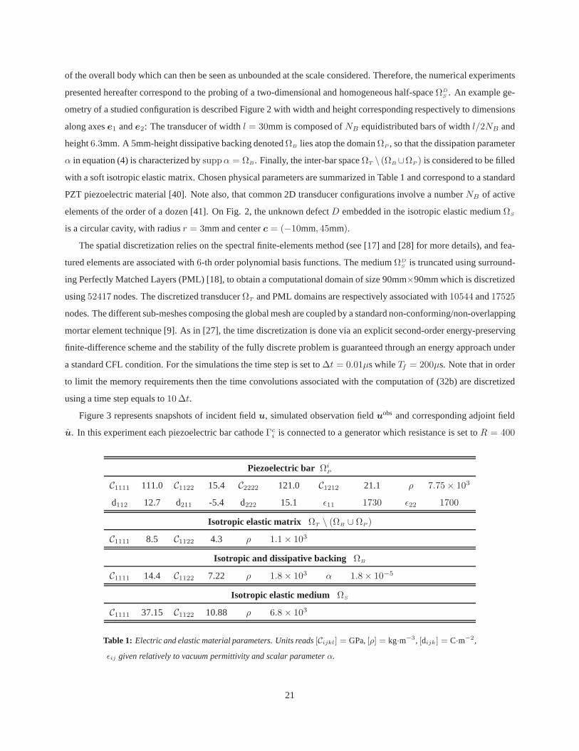
Piezoelectric bar ΩiP

C1111 111.0 C1122 15.4 C2222 121.0 C1212 21.1 ρ 7.75× 103

d112 12.7 d211 -5.4 d222 15.1 ǫ11 1730 ǫ22 1700

Isotropic elastic matrix ΩT \ (ΩB ∪ ΩP )

C1111 8.5 C1122 4.3 ρ 1.1× 103

Isotropic and dissipative backing ΩB

C1111 14.4 C1122 7.22 ρ 1.8× 103 α 1.8× 10−5

Isotropic elastic medium ΩS

C1111 37.15 C1122 10.88 ρ 6.8× 103

Table 1: Electric and elastic material parameters. Units reads[Cijkl] = GPa, [ρ] = kg·m−3, [dijk] = C·m−2,

ǫij given relatively to vacuum permittivity and scalar parameter α.

21

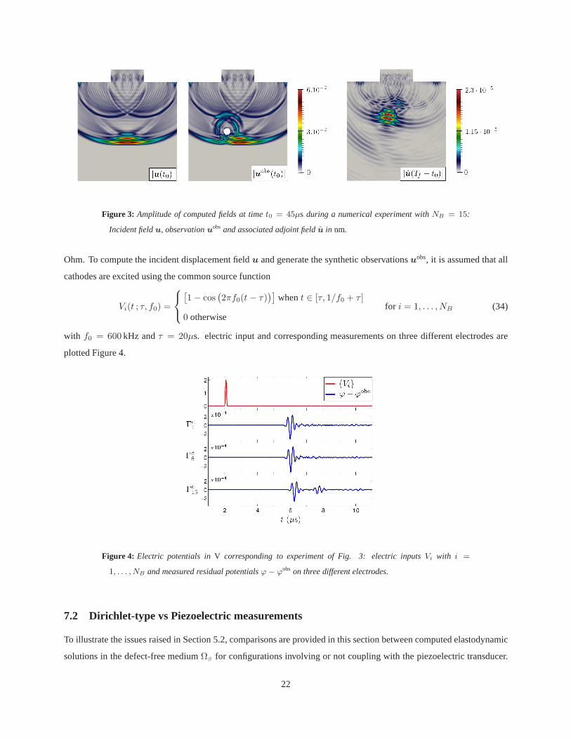
Figure 3: Amplitude of computed fields at timet0 = 45µs during a numerical experiment withNB = 15:

Incident fieldu, observationuobs and associated adjoint fieldu in nm.

Ohm. To compute the incident displacement fieldu and generate the synthetic observationsuobs, it is assumed that all

cathodes are excited using the common source function

Vi(t ; τ, f0) =

[

1− cos(

2πf0(t− τ))]

whent ∈ [τ, 1/f0 + τ ]

0 otherwisefor i = 1, . . . , NB (34)

with f0 = 600 kHz andτ = 20µs. electric input and corresponding measurements on three different electrodes are

plotted Figure 4.

Figure 4: Electric potentials inV corresponding to experiment of Fig. 3: electric inputsVi with i =

1, . . . , NB and measured residual potentialsϕ− ϕobs on three different electrodes.

7.2 Dirichlet-type vs Piezoelectric measurements

To illustrate the issues raised in Section 5.2, comparisonsare provided in this section between computed elastodynamic

solutions in the defect-free mediumΩS for configurations involving or not coupling with the piezoelectric transducer.

22

(a) Free-surface b.c.: Time-reversed incident fieldu(Tf − t) (b) Dirichlet-type measurements: Adjoint fieldu(t)

(c) Piezoelectric b.c.: Time-reversed incident fieldu(Tf − t) (d) Piezoelectric measurements: Adjoint fieldu(t)

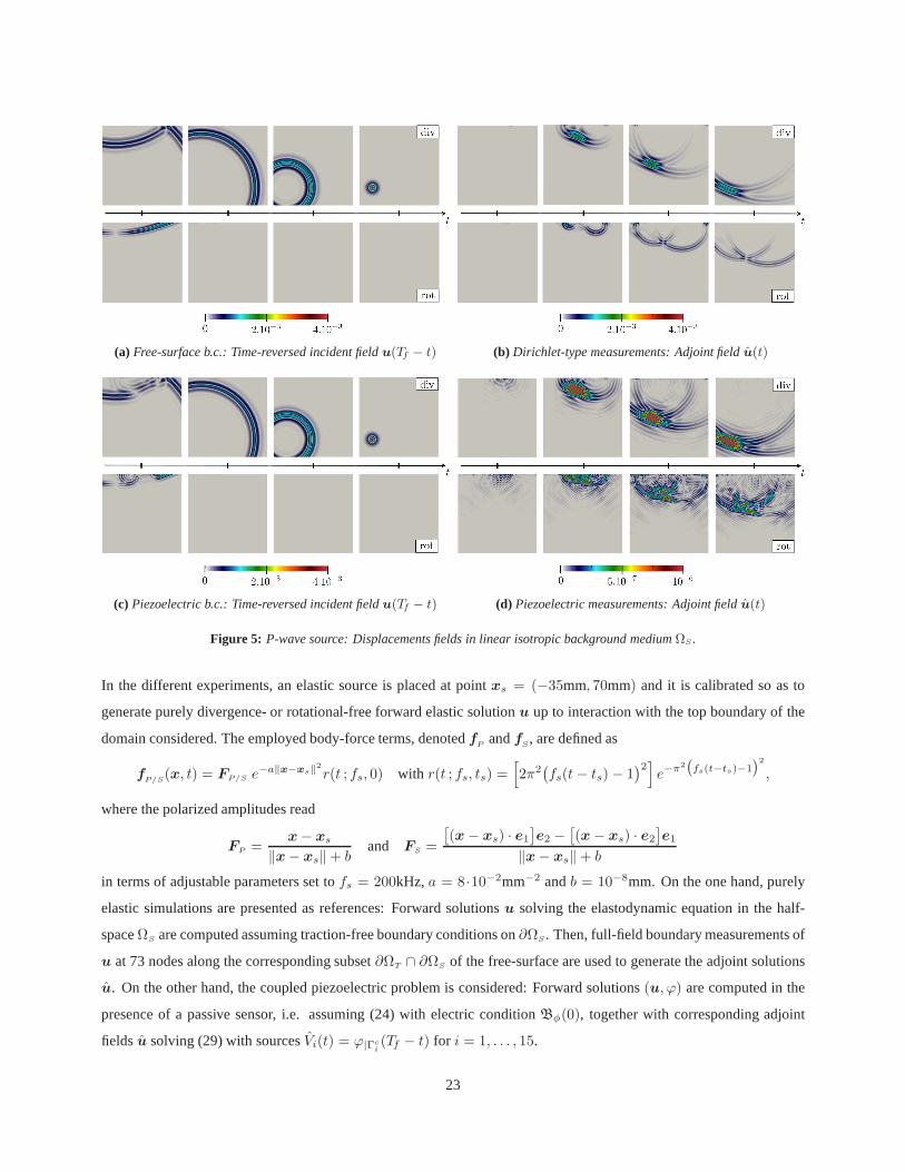
Figure 5: P-wave source: Displacements fields in linear isotropic background mediumΩS .

In the different experiments, an elastic source is placed atpoint xs = (−35mm, 70mm) and it is calibrated so as to

generate purely divergence- or rotational-free forward elastic solutionu up to interaction with the top boundary of the

domain considered. The employed body-force terms, denotedfP andfS, are defined as

fP/S(x, t) = FP/S e−a‖x−xs‖

2

r(t ; fs, 0) with r(t ; fs, ts) =[

2π2(

fs(t− ts)− 1)2]

e−π2

(

fs(t−ts)−1)

2

,

where the polarized amplitudes read

FP =x− xs

‖x− xs‖+ band FS =

[

(x− xs) · e1]

e2 −[

(x− xs) · e2]

e1

‖x− xs‖+ b

in terms of adjustable parameters set tofs = 200kHz, a = 8·10−2mm−2 andb = 10−8mm. On the one hand, purely

elastic simulations are presented as references: Forward solutionsu solving the elastodynamic equation in the half-

spaceΩS are computed assuming traction-free boundary conditions on∂ΩS. Then, full-field boundary measurements of

u at 73 nodes along the corresponding subset∂ΩT ∩ ∂ΩS of the free-surface are used to generate the adjoint solutions

u. On the other hand, the coupled piezoelectric problem is considered: Forward solutions(u, ϕ) are computed in the

presence of a passive sensor, i.e. assuming (24) with electric conditionBφ(0), together with corresponding adjoint

fieldsu solving (29) with sourcesVi(t) = ϕ|Γci(Tf − t) for i = 1, . . . , 15.

23

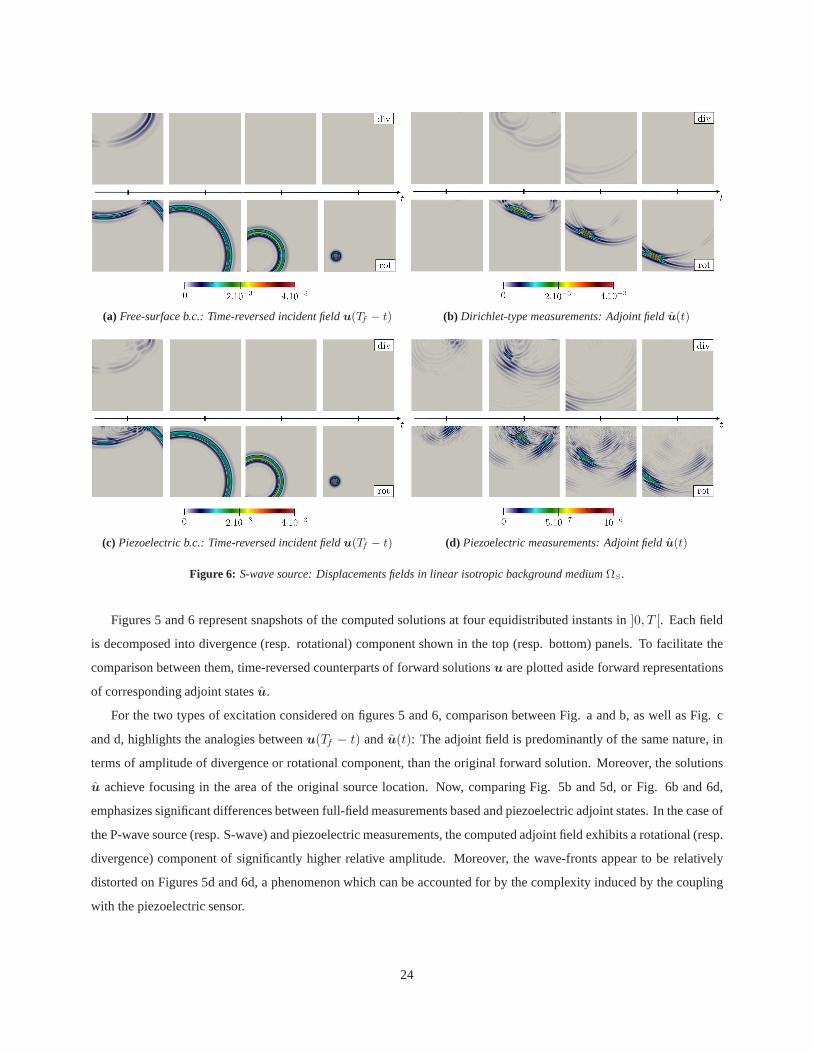
(a) Free-surface b.c.: Time-reversed incident fieldu(Tf − t) (b) Dirichlet-type measurements: Adjoint fieldu(t)

(c) Piezoelectric b.c.: Time-reversed incident fieldu(Tf − t) (d) Piezoelectric measurements: Adjoint fieldu(t)

Figure 6: S-wave source: Displacements fields in linear isotropic background mediumΩS .

Figures 5 and 6 represent snapshots of the computed solutions at four equidistributed instants in]0, T [. Each field

is decomposed into divergence (resp. rotational) component shown in the top (resp. bottom) panels. To facilitate the

comparison between them, time-reversed counterparts of forward solutionsu are plotted aside forward representations

of corresponding adjoint statesu.

For the two types of excitation considered on figures 5 and 6, comparison between Fig. a and b, as well as Fig. c

and d, highlights the analogies betweenu(Tf − t) andu(t): The adjoint field is predominantly of the same nature, in

terms of amplitude of divergence or rotational component, than the original forward solution. Moreover, the solutions

u achieve focusing in the area of the original source location. Now, comparing Fig. 5b and 5d, or Fig. 6b and 6d,

emphasizes significant differences between full-field measurements based and piezoelectric adjoint states. In the case of

the P-wave source (resp. S-wave) and piezoelectric measurements, the computed adjoint field exhibits a rotational (resp.

divergence) component of significantly higher relative amplitude. Moreover, the wave-fronts appear to be relatively

distorted on Figures 5d and 6d, a phenomenon which can be accounted for by the complexity induced by the coupling

with the piezoelectric sensor.

24

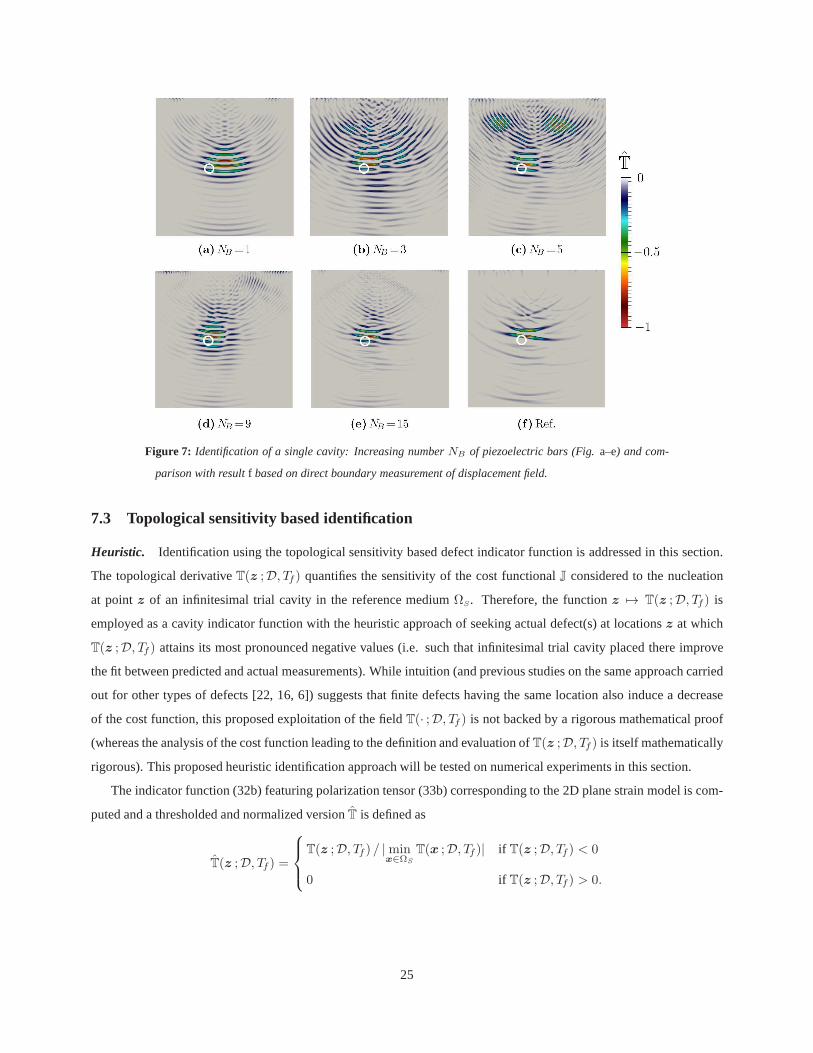
Figure 7: Identification of a single cavity: Increasing numberNB of piezoelectric bars (Fig.a–e) and com-

parison with resultf based on direct boundary measurement of displacement field.

7.3 Topological sensitivity based identification

Heuristic. Identification using the topological sensitivity based defect indicator function is addressed in this section.

The topological derivativeT(z ;D, Tf) quantifies the sensitivity of the cost functionalJ considered to the nucleation

at pointz of an infinitesimal trial cavity in the reference mediumΩS. Therefore, the functionz 7→ T(z ;D, Tf) is

employed as a cavity indicator function with the heuristic approach of seeking actual defect(s) at locationsz at which

T(z ;D, Tf) attains its most pronounced negative values (i.e. such thatinfinitesimal trial cavity placed there improve

the fit between predicted and actual measurements). While intuition (and previous studies on the same approach carried

out for other types of defects [22, 16, 6]) suggests that finite defects having the same location also induce a decrease

of the cost function, this proposed exploitation of the fieldT(· ;D, Tf ) is not backed by a rigorous mathematical proof

(whereas the analysis of the cost function leading to the definition and evaluation ofT(z ;D, Tf) is itself mathematically

rigorous). This proposed heuristic identification approach will be tested on numerical experiments in this section.

The indicator function (32b) featuring polarization tensor (33b) corresponding to the 2D plane strain model is com-

puted and a thresholded and normalized versionT is defined as

T(z ;D, Tf) =

T(z ;D, Tf) / |minx∈ΩS

T(x ;D, Tf)| if T(z ;D, Tf) < 0

0 if T(z ;D, Tf) > 0.

25

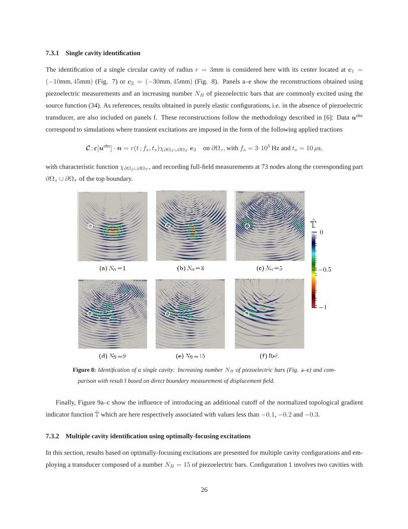
7.3.1 Single cavity identification

The identification of a single circular cavity of radiusr = 3mm is considered here with its center located atc1 =

(−10mm, 45mm) (Fig. 7) orc2 = (−30mm, 45mm) (Fig. 8). Panels a–e show the reconstructions obtained using

piezoelectric measurements and an increasing numberNB of piezoelectric bars that are commonly excited using the

source function (34). As references, results obtained in purely elastic configurations, i.e. in the absence of piezoelectric

transducer, are also included on panels f. These reconstructions follow the methodology described in [6]: Datauobs

correspond to simulations where transient excitations areimposed in the form of the following applied tractions

C :ε[uobs] · n = r(t ; fs, ts)χ∂ΩS∪∂ΩT e2 on∂ΩS,with fs = 3·105 Hz andts = 10µs,

with characteristic functionχ∂ΩS∪∂ΩT , and recording full-field measurements at 73 nodes along thecorresponding part

∂ΩS ∪ ∂ΩT of the top boundary.

Figure 8: Identification of a single cavity: Increasing numberNB of piezoelectric bars (Fig.a–e) and com-

parison with resultf based on direct boundary measurement of displacement field.

Finally, Figure 9a–c show the influence of introducing an additional cutoff of the normalized topological gradient

indicator functionT which are here respectively associated with values less than−0.1, −0.2 and−0.3.

7.3.2 Multiple cavity identification using optimally-focusing excitations

In this section, results based on optimally-focusing excitations are presented for multiple cavity configurations andem-

ploying a transducer composed of a numberNB = 15 of piezoelectric bars. Configuration 1 involves two cavities with

26

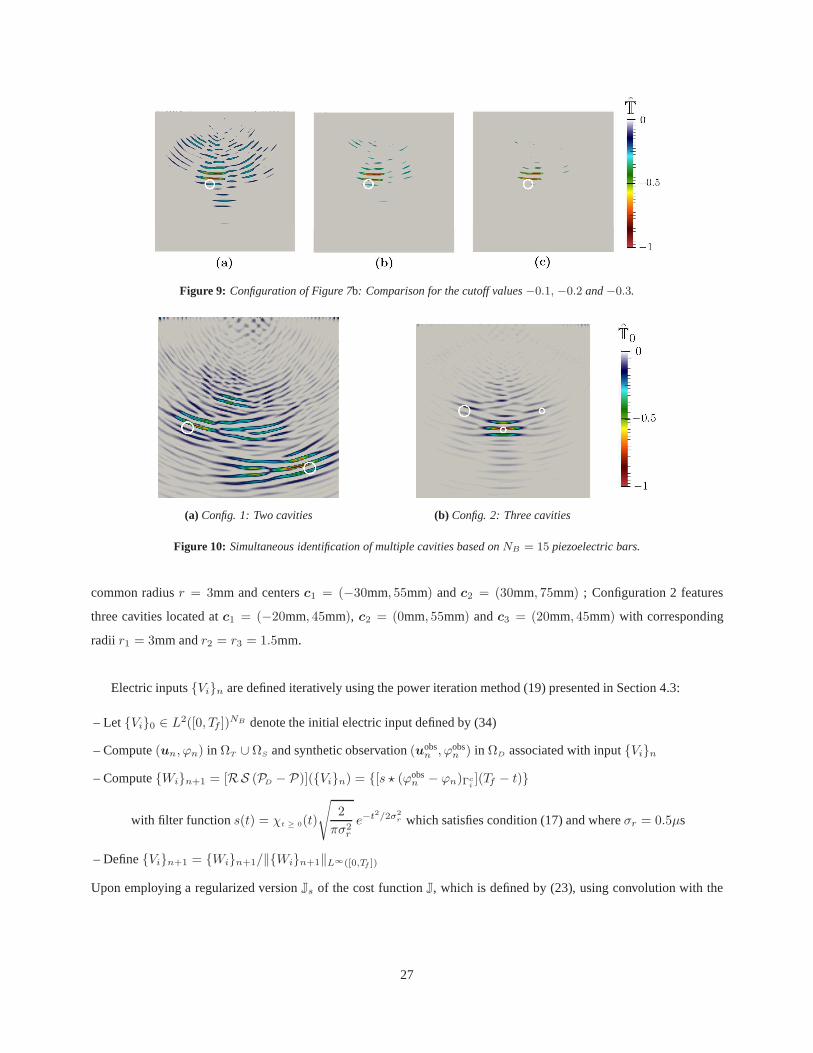
Figure 9: Configuration of Figure 7b: Comparison for the cutoff values−0.1, −0.2 and−0.3.

(a) Config. 1: Two cavities (b) Config. 2: Three cavities

Figure 10: Simultaneous identification of multiple cavities based onNB = 15 piezoelectric bars.

common radiusr = 3mm and centersc1 = (−30mm, 55mm) andc2 = (30mm, 75mm) ; Configuration 2 features

three cavities located atc1 = (−20mm, 45mm), c2 = (0mm, 55mm) andc3 = (20mm, 45mm) with corresponding

radii r1 = 3mm andr2 = r3 = 1.5mm.

Electric inputsVin are defined iteratively using the power iteration method (19) presented in Section 4.3:

– LetVi0 ∈ L2([0, Tf ])NB denote the initial electric input defined by (34)

– Compute(un, ϕn) in ΩT ∪ ΩS and synthetic observation(uobsn , ϕobs

n ) in ΩD associated with inputVin

– ComputeWin+1 = [RS (PD − P)](Vin) = [s ⋆ (ϕobsn − ϕn)Γc

i](Tf − t)

with filter functions(t) = χt ≥ 0(t)

√

2

πσ2r

e−t2/2σ2

r which satisfies condition (17) and whereσr = 0.5µs

– DefineVin+1 = Win+1/‖Win+1‖L∞([0,Tf ])

Upon employing a regularized versionJs of the cost functionJ, which is defined by (23), using convolution with the

27

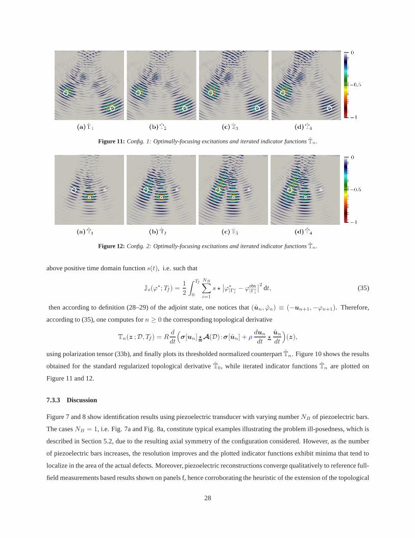
Figure 11: Config. 1: Optimally-focusing excitations and iterated indicator functionsTn.

Figure 12: Config. 2: Optimally-focusing excitations and iterated indicator functionsTn.

above positive time domain functions(t), i.e. such that

Js(ϕ∗;Tf) =

1

2

∫ Tf

0

NB∑

i=1

s ⋆∣

∣ϕ∗|Γc

i− ϕobs

|Γci

∣

∣

2dt, (35)

then according to definition (28–29) of the adjoint state, one notices that(un, ϕn) ≡ (−un+1,−ϕn+1). Therefore,

according to (35), one computes forn ≥ 0 the corresponding topological derivative

Tn(z ;D, Tf) = Rd

dt

(

σ[un] ⋆A(D) :σ[un] + ρdun

dt⋆un

dt

)

(z),

using polarization tensor (33b), and finally plots its thresholded normalized counterpartTn. Figure 10 shows the results

obtained for the standard regularized topological derivative T0, while iterated indicator functionsTn are plotted on

Figure 11 and 12.

7.3.3 Discussion

Figure 7 and 8 show identification results using piezoelectric transducer with varying numberNB of piezoelectric bars.

The casesNB = 1, i.e. Fig. 7a and Fig. 8a, constitute typical examples illustrating the problem ill-posedness, which is

described in Section 5.2, due to the resulting axial symmetry of the configuration considered. However, as the number

of piezoelectric bars increases, the resolution improves and the plotted indicator functions exhibit minima that tendto

localize in the area of the actual defects. Moreover, piezoelectric reconstructions converge qualitatively to reference full-

field measurements based results shown on panels f, hence corroborating the heuristic of the extension of the topological

28

sensitivity approach to piezoelectric-sensor based measurements. The identification of the out-of-axis cavity of Fig. 8

is deteriorated relatively to Fig. 7, a phenomenon which canbe accounted for by the characteristic in-axis transducer

emission of elastic energy which is illustrated Fig. 3. Finally, as shown on Figure 9 the reconstruction legibility can

be enhanced by introducing an additional cutoff parameter which allows to locate precisely the global minimum of the

indicator function.

For the cases of simultaneous identifications of multiple cavity, Figure 10 illustrates the influence of the distance

between obstacles and of their relative scattering strengths, a factor which is correlated to the assumed illumination.

The two well-separated cavities of Fig. 10a are relatively well located by the global minima of the indicator function,

whereas on Fig. 10b the different obstacles are not correctly identified. One may also note the relative spreading of the

indicator function of Fig. 10a ; These artefacts may be associated with the adjoint field features and discrepancy from

its full-field measurements based counterpart that are described in Section 7.2.

When optimally-focusing excitations are used to probe the media considered, as in Fig. 11 and 12, the identification

results are significantly improved. Comparison between indicator functionsT0 andT1 on Fig. 10a and 11a highlights

that a single iteration of the proposed method reduces remarkably the previously observed artefacts. Concerning iterated

illuminations with corresponding indicator functions plotted Fig. 11a–d and 12a–d, then global minima tend to localize

in the area of the strongest scatterers in accordance with the expected properties of the approach that are discussed in

Section 4.3. Note that the geometric spreading of the indicator function increases with iterations, a feature which may

be caused by the expected convergence of the iterated adjoint field towards a harmonic solution, a phenomenon which

is described in [2] in a slightly different context.

8 Conclusions

This study concerns the investigation of an inverse scattering problem revolving around the identification of defects em-

bedded in elastic solids from piezoelectric sensor-based electric measurements. A fundamental piezoelectric reciprocity

identity is proven and applied to a specific transducer model. The characteristic features of such inverse problem associ-

ated with electric data are discussed and a comparison is drawn with commonly used direct displacement field boundary

measurements in full, or partial, waveform. Along the linesof iterative time reversal techniques, a construction pro-

cedure of optimally-focusing electric inputs is presentedand implemented. In the context of traction-free cavities,

extraction of the informations encapsulated in the available measurements is investigated by way of an adjoint-field

based topological sensitivity approach, which uses the derived reciprocity relations, leading to the construction and the

non-iterative computation of a defect indicator function.The proposed approach is deployed within the framework of a

spectral finite-elements computational platform in order to assess its capabilities and performances on 2D examples. For

completeness, the comparison is made with topological sensitivity-based reconstructions featuring full-field boundary

measurements.

Theoretical work remains to be done to provide proper mathematical backing to the interpretation of the indicator

29

function (32b), as well as to characterize the eigensystem of the iterated time reversal operator introduced in Theorem

4.1. Future studies will also encompass practical and computational investigations of the expected straightforward

generalization of this work to other types of defects, and extensions of the proposed approach in association with

topological sensitivity-based indicator functions developed for anisotropic and heterogeneous elastic solids. Finally,

addressing numerically reconstruction problems associated with 3D configurations remains to be done. To do so, the

design of a specific algorithm aiming at limiting the memory cost associated with the time-domain convolutions in

equation (32b) is needed.

References

[1] J. D. Achenbach.Reciprocity in elastodynamics. Cambridge Monographs on Mechanics. Cambridge University

Press, Cambridge, 2003.

[2] C. Ben Amar and C. Hazard. Time reversal and scattering theory for time-dependent acoustic waves in a homoge-

neous medium.IMA J. Appl. Math., 76:938–955, 2011.

[3] H. Ammari and H. Kang.Polarization and moment tensors with applications to inverse problems and effective

medium theory, volume 162 ofApplied Mathematical Sciences. Springer, Berlin, 2007.

[4] T. Arens. Linear sampling methods for 2D inverse elasticwave scattering.Inverse Problems, 17:1445–1464, 2001.

[5] B. A. Auld. General electromechanical reciprocity relations applied to the calculation of elastic wave scattering

coefficients.Wave Motion, 1:3–10, 1979.

[6] C. Bellis and M. Bonnet. A FEM-based topological sensitivity approach for fast qualitative identification of

buried cavities from elastodynamic overdetermined boundary data.International Journal of Solids and Structures,

47(9):1221–1242, 2010.

[7] C. Bellis and M. Bonnet. Qualitative identification of cracks using 3D transient elastodynamic topological deriva-

tive: Formulation and FE implementation.Comput. Methods Appl. Mech. Engrg., 253:89–105, 2013.

[8] C. Bellis and S. Imperiale. Dynamical one-dimensional models of passive piezoelectric sensors.Math. Mech.

Solids, pages 1–26, 2012.

[9] A. Bendali and Y. Boubendir. Non-overlapping domain decomposition method for a nodal finite element method.

Numerische Mathematik, 103(4):515–537, 2006.

[10] M. Bonnet. Topological sensitivity for 3D elastodynamics and acoustic inverse scattering in the time domain.

Comput. Methods Appl. Mech. Engrg., 195:5239–5254, 2006.

[11] M. Bonnet and A. Constantinescu. Inverse problems in elasticity. Inverse Problems, 21:R1–R50, 2005.

30

[12] M. Bonnet and B. B. Guzina. Sounding of finite solid bodies by way of topological derivative.Int. J. Num. Meth.

in Eng., 61:2344–2373, 2004.

[13] H. D. Bui, A. Constantinescu, and H. Maigre. Numerical identification of linear cracks in 2D elastodynamics using

the instantaneous reciprocity gap.Inverse Problems, 20:993–1001, 2004.

[14] F. Cakoni and D. Colton.Qualitative methods in inverse scattering theory. Springer, Berlin, 2006.

[15] A. Charalambopoulos, A. Kirsch, K. A. Anagnostopoulos, D. Gintides, and K. Kiriaki. The factorization method

in inverse elastic scattering from penetrable bodies.Inverse Problems, 23:27–51, 2007.

[16] I. Chikichev and B. B. Guzina. Generalized topologicalderivative for the navier equation and inverse scattering in

the time domain.Comp. Meth. Appl. Mech. Engng., 197:4467–4484, 2008.

[17] G. Cohen.Higher-order numerical methods for transient wave equations. Springer, 2001.

[18] E. Demaldent and S. Imperiale. Perfectly matched transmission problems with absorbing layers: Application to

anisotropic acoustics.Submitted, 2012.

[19] N. Dominguez, V. Gibiat, and Y. Esquerre. Time domain topological gradient and time reversal analogy: an inverse

method for ultrasonic target detection.Wave Motion, 42(1):31–52, 2005.

[20] L. L. Foldy and H. Primakoff. A general theory of passivelinear electroacoustic transducers and the electroacoustic

reciprocity theorem. I.J. Acoust. Soc. Am., 17:109–120, 1945.

[21] S. Garreau, P. Guillaume, and M. Masmoudi. The topological asymptotic for pde systems: the elasticity case.

SIAM J. Control Optim., 39:1756–1778, 2001.

[22] B.B. Guzina and M. Bonnet. Topological derivative for the inverse scattering of elastic waves.Quart. J. Mech.

Appl. Math., 57:161–179, 2004.

[23] E. J. Haug, K. K. Choi, and V. Komkov.Design Sensitivity Analysis of Structural Systems. Academic Press, 1986.

[24] C. Hazard and K. Ramdani. Slective acoustic focusing using time-harmonic reversal mirrors.SIAM J. Appl. Math.,

64:1657–1676, 2004.

[25] T. Ikeda.Fundamentals of piezoelectricity. Oxford University Press, 1990.

[26] S. Imperiale. Etude mathématique et numérique de capteurs piézoélectriques. PhD thesis, Université Paris

Dauphine, France, 2012.

[27] S. Imperiale and P. Joly. Mathematical and numerical modelling of piezoelectric sensors.ESAIM: Mathematical

Modelling and Numerical Analysis, 46:875–909, 2012.

31

[28] D. Komatitsch and J. Tromp. Introduction to the spectral element method for three-dimensional seismic wave

propagation.Geophysical Journal International, 139(3):806–822, 2002.

[29] R. Lerch. Simulation of piezoelectric devices by two-and three-dimensional finite elements.IEEE Trans. Ultra.

Ferr. Freq. Cont., 37:233–247, 2002.

[30] J. Y. Li. Uniqueness and reciprocity theorems for linear thermo-electro-magneto-elasticity.Quart. J. Mech. Appl.

Math., 56:35–43, 2003.

[31] S. Nintcheu Fata and B. B. Guzina. A linear sampling method for near-field inverse problems in elastodynamics.

Inverse Problems, 20:713–736, 2004.

[32] W. Nowacki. A reciprocity theorem for coupled mechanical and thermoelectric fields in piezoelectric crystals. In

Proceedings of Vibration Problems, volume 6, pages 3–11, Warsaw, 1965.

[33] A. A. Oberai, G. R. Feijoo, and P.E. Barbone. Lanczos-iterated time reversal.J. Acoust. Soc. Am. Exp. Let.,

125:70–76, 2009.

[34] R. Pike and P. Sabatier.Scattering: Scattering and Inverse Scattering in Pure and Applied Science. Academic

Press, 2002.

[35] R. E. Plessix, Y. H. De Roeck, and G. Chavent. Waveform inversion of reflection seismic data for kinematic

parameters by local optimization.SIAM J. Sci. Comput., 20:1033–1052, 1999.

[36] C. Prada and M. Fink. Eigenmodes of the time reversal operator: A solution to selective focusing in multiple target

media.Wave Motion, 20:151–163, 1994.

[37] C. Prada, S. Manneville, D. Spoliansky, and M. Fink. Decomposition of the time reversal operator: Application to

detection and selective focusing on two scatterers.J. Acoust. Soc. Am., 99:2067–2076, 1996.

[38] C. Prada, J. L. Thomas, and M. Fink. The iterative time reversal process: Analysis of the convergence.J. Acoust.

Soc. Am., 97:62–71, 1995.

[39] I. T. Rekanos, T. V. Yioultsis, and T. D. Tsiboukis. Inverse scattering using the finite element method and a

nonlinear optimization technique.IEEE Transactions on microwave theory and techniques, 47:336–344, 1999.

[40] D. Royer and E. Dieulesaint.Elastic waves in solids I. Free and guided propagation. Springer, 2000.

[41] D. Royer and E. Dieulesaint.Elastic waves in solids II. Generation, acousto-optic interaction, applications.

Springer, 2000.

[42] Andrieux S., A. Ben Abda, and Bui H. D. Reciprocity principle and crack identification.Inverse Problems,

15:59–65, 1999.

32

[43] J. Salençon.Handbook of continuum mechanics: General concepts, thermoelasticity. Springer, 2001.

[44] L. Schmerr Jr and S. J. Song.Ultrasonic nondestructive evaluation systems. Springer, 2007.

[45] J. Sokolowski and A. Zochowski. On the topological derivative in shape optimization.SIAM J. Control Optim.,

37:1251–1272, 1999.

33