CEE DP 120

The Timing of Parental Income and Child Outcomes:

The Role of Permanent and Transitory Shocks

Emma Tominey

October 2010

ISSN 2045-6557

Published by

Centre for the Economics of Education

London School of Economics

Houghton Street

London WC2A 2AE

© E.P. Tominey, submitted October 2010

All rights reserved. No part of this publication may be reproduced, stored in a retrieval

system or transmitted in any form or by any means without the prior permission in writing of

the publisher nor be issued to the public or circulated in any form other than that in which it

is published.

Requests for permission to reproduce any article or part of the Working Paper should be

sent to the editor at the above address.

The Centre for the Economics of Education is an independent multidisciplinary research

centre. All errors and omissions remain the authors.

The Timing of Parental Income and Child Outcomes:

The Role of Permanent and Transitory Shocks

Emma Tominey

1. Introduction 2

2. The Norwegian Setting 6

3. Data 7

4. Income Process in Norway 9

5. Empirical Strategy 11

Income process 11 Child human capital equation 12 Identification 12

6. Results 14

Income shocks 14 Distribution of income shocks 15 Effects of shocks on adolescent outcomes 16 Paternal income 19 Liquidity constrained sample 20

7. Robustness Checks 22

Assuming MA (2) process for transitory income 22 Are the shocks unexpected? 22 Siblings 24

8. Conclusion 24

Figures 26

Tables 32

Annex 38

References 39

Acknowledgments

Emma Tominey is a Lecturer at the Department of Economics and Related Studies, University

of York, and an Associate of the Centre for the Economics of Education.

1 Introduction

How do shocks to parental income drive adolescent human capital, such as university atten-

dance, IQ and health? Unexpected changes to family income may have a predictable e¤ect

on child adolescent outcomes, by shifting the money parents spend on human capital invest-

ments in their children. The extent to which consumers insure themselves against changes

in income has been well documented in the economics literature,2 however little is known

about how the evolution of household income drives the human capital of their children. This

paper �lls the gap and makes two important innovations by �rstly estimating the e¤ect of

shocks across the life cycle of childhood, from age 1-16 and secondly distinguishing between

income shocks that are permanent and transitory.

Does human capital acquisition respond to income shocks in a similar manner as con-

sumption? Theory posits that income shocks which are persistent have distinct e¤ects on

consumption from shocks that are purely transitory3. According to the Permanent Income

Hypothesis (PIH), an income shock transmits to consumption through its change in lifetime

household wealth. Consider a permanent shock of a promotion, for example. This shock

will raise contemporaneous income but also income in all future periods. This means that

an early permanent income shock will have a larger e¤ect upon parental investment (and

therefore child outcomes) than one realised later in the child�s lifetime. The reason is that

ceteris paribus, a permanent shock realised at birth will drive more future income realisations

than a shock at age 16.

On the other hand, the PIH predicts a di¤erent transmission of transitory income shocks

to child human capital. A transitory shock such as a bonus changes contemporaneous income

and potentially income for a few future periods but is mean reverting. Under incomplete

insurance, unexpected �uctuations in transitory income alter lifetime wealth by the product

of 1/T and the value of the shock.4 These shocks are absorbed through borrowing or saving

and, both consumption and parental investment are smoothed. Consequently, the e¤ect of

transitory income shocks to the eventual stock of child human capital is lower than that

for permanent shocks, but this di¤erence decreases across child age. If human capital accu-

mulation behaves similarly to consumption, I expect to �nd that permanent income shocks

have an e¤ect on adolescent outcomes which declines in the age of the child when shocks are

realised and transitory income shocks have a small but constant e¤ect.

2Deaton (1992) provides a good summary. Blundell & Preston (1998), Attanasio et al (2002), Blundell etal (2008) examine consumption responses to income changes and Adda et al (2009) look at health responsesto income shocks.

3See Friedman (1957).4T denotes the total periods of labour market participation of parents.

2

The PIH thus predicts heterogeneous e¤ects across the child life cycle. Indeed, a recent

literature suggests that the determinant of adolescent college enrolment is not contempora-

neous income, but rather the �ow of parental income across childhood. Cameron & Heckman

(2001), Keane & Wolpin (2001) and Cameron & Taber (2004) argue that it is not the pres-

ence of credit constraints at the point in time when individuals decide to enter college that

drives that decision, but rather a binding lifetime credit constraints which alter human cap-

ital investment throughout childhood. As such this paper analyses the role of income shocks

at every age of childhood, from birth up until age 16.

I explore heterogeneity in the time pro�le of the e¤ect of transitory income shocks upon

outcomes, by focusing on liquidity constrained households. With imperfect access to credit

markets, liquidity constrained agents are unable to borrow or save in order to smooth tran-

sitory income shocks su¢ ciently. Consequently I would expect to �nd a larger e¤ect of

transitory income shock in liquidity constrained households.

The decomposition of the e¤ect of family income shocks upon child outcomes by the

durability of the shock and the age of the child, has not currently been explored by literature.

One potential reason is a lack of adequate data. The data in this paper takes the population

of around 600,000 Norwegian children, born in the 1970s and tracked through to 2006,

which provides in depth information on annual household income plus a range of adolescent

outcomes, including years of schooling, high school dropout, university attendance and IQ

and health test scores from a set of army tests for males.

There are of course contributions from the empirical literature along several relevant

dimensions. A literature suggests that a potential mechanism through which parental income

shocks drive child outcomes is through a shift in parental investments in child human capital.5

The e¤ect of speci�c shocks to the household upon child outcomes has been investigated in

a number of papers6. Akee et al (2010) found that the age of the child when the shock

was realised strongly conditioned the e¤ect of that shock. In particular, the e¤ect of an

exogeneous and permanent government transfer to households had a larger e¤ect on schooling

and crime outcomes for children with six, rather than two years exposure to the higher

income.

Interestingly, the predictions of the e¤ect of timing of income levels di¤ers markedly from

the timing of income shocks. In the absence of credit constraints, a simple model predicts

5Cunha & Heckman (2007, 2008) and Cunha et al (2010) distinguish between �nancial such as books,private tuition and time investments such as reading to children and trips to a museum. A negative incomeshock of unemployment could lead parents to change money or time spent on their children, e.g. cancel aprivate tutor in the one case or help the child with homework in the other. Ginja (2009) �nds that investmentgoods are responsive to an unexpected change in family income.

6There are many examples. One is by Chen et al (2009), who explore the e¤ect of unexpected parentaldeath upon the probability of enrolling in college, in Taiwan.

3

that parental investment in human capital does not respond to the timing of income, given

permanent income. Parents would optimally borrow and save to smooth the e¤ect of the

timing of income.7 However, in this paper the model is extended to allow for income uncer-

tainty. Unexpected changes in income lead to predictable changes in parental investment

(which depend upon the durability of the income shock and child age) and therefore child

adolescent outcomes.

Finally, it is worth noting that a component of the e¤ect of income shocks is parental

insurance. If children are fully insured against the income shock, the data will reveal a zero

e¤ect across child age. A number of papers have established that the human capital of young

adults is partially insured by their parents.8 For example, Kaplan (2007) �nds that youths

faced with labour market risk call upon both �nancial transfers and co-residence as insurance

mechanisms and Rosenzweig & Wolpin (1993) suggest that parental insurance is required in

addition to government insurance, even against anticipated income shocks.

There are important policy implications inherent in this study. Cunha (2005) and Cunha

& Heckman (2007, 2008) posit that parental investment will be more e¤ective early in the

lifetime of a child. Firstly, neurological arguments suggest that early investments into cog-

nitive ability will have a higher return than later investment9. This combined with the

suggestion that there are dynamic complementarities in the return to investment, such that

the return to early (late) investment is increasing in the level of late (early) investment,

points e¤ective policy making towards the early years. Family income is arguably easier to

target by governments than parental investment and as such, this paper estimates the value

of government insurance for households with children, against unexpected changes to income.

As noted above, the largest e¤ect is expected for permanent shocks early in the lifetime of a

child. However, it is transitory shocks which provide the relevant policy experiment, as they

are insurable by government whereas permanent shocks in general, are not.10

The methodology used in this paper follows two stages. Firstly, a structural model of

the parental income process decomposes income shocks into permanent and transitory com-

ponents. Secondly, the reduced form e¤ects of the separate shocks, experienced at di¤erent

ages in the child�s life, on their eventual child capital levels are estimated.11

7Carneiro et al (2010) do indeed �nd evidence of a relatively �at pro�le of the e¤ect of the timing ofincome, although there is some evidence of dynamic complementarity in the return. On the other hand,Jenkins & Schluter (2002) �nd a higher return to late, and Levy & Duncan (2000) �nds a higher return toearly years income.

8See for example Hayashi et al (1996), Martins & Villanueva (2009) and Becker et al (2010).9For example, the cohort-ranking of IQ is set very early, at around age 5.10There are of course exceptions, such as governments tend to guarantee a subsistence level of income and

additionally insurance against loss of income through disability.11Paxson (1992), Shapiro & Slemrod (1995), Parker (1999) and Souleles (1999) adopt an alternative

methodology by exploiting exogeneous variation in income to identify the role of transitory income shocks

4

A necessary �rst step therefore is to gather empirical evidence as to the income process

that is applied to the structural model. I use a panel of around 400,000 parents observed

across a 30 year period to estimate the autocovariances of income growth. Permanent income

is assumed to follow a random walk and the evidence suggests that transitory income is

best described by an MA(1) or MA(2) process. Next, deviations of household income from

the life cycle trend are predicted in each year of child life. Moment conditions from the

income process allow a decomposition into permanent and transitory income shocks from

early childhood to adolescence. These are estimated at the level of the cohort within a

labour market.12 Finally, the e¤ect of both types of shock, realised across the child life cycle,

is estimated in a reduced form equation on the eventual stock of adolescent human capital

outcomes. The model allows for correlation between an initial condition in household income

and a parental �xed e¤ect in child human capital. The identi�cation assumption in the �rst

stage decomposition is that second order moments of the permanent and transitory income

shocks di¤er across child age, cohorts and labour markets, but that the e¤ect of these shocks

varies only across child age. The second stage identi�cation assumption is that estimated

income shocks are exogeneous and unexpected by households. The former is based upon

evidence from 400,000 households across 30 years and the latter is tested in two robustness

checks.

The data indicate a strong and signi�cant correlation between the initial condition and

child outcomes. A rise in initial income levels by 1 standard deviation raises child human cap-

ital by up to 0.4 standard deviations (equivalent, for example, to nearly a year of schooling).

This shows that family background matters - there is signi�cant dispersion in outcomes for

the sample of Norwegian children, determined at the start of their lifetime. For all outcomes

except health, the e¤ect of a household permanent income shock is signi�cant and declines

across child age, as predicted by the PIH. However there is volatility in this relationship,

which may be picking up changes in maternal labour supply. Mothers have less attachment

to the labour market and their labour supply is more sensitive, for example to children start-

ing school. By focusing just on paternal income, noise in the decline is smoothed out for

all outcomes. The di¤erence in the health outcome is likely due to crude measurement in

the data.13 In general, permanent shocks to paternal income have a large e¤ect early in the

lifetime of the child and this e¤ect falls across child age, to zero at age 16.

upon consumption. For this paper, it would be very cumbersome, if not impossible, to �nd strong instrumentsfor both permanent and transitory income shocks throughout the lifetime of children.12The method is a slight adaptation to Mo¢ tt & Gottschalk (1995), Meghir & Pistaferri (2004) and

Blundell et al (2008) and similar to Jappelli & Pistaferri (2008).13In all speci�cations, for both permanent and transitory shocks, there is a noisy and insigni�cant e¤ect

of shocks on health.

5

For all outcomes, transitory income shocks have a small and constant e¤ect across child

age. This suggests that parents are optimising, by smoothing parental investment against

transitory shocks in a similar manner to consumption smoothing.

However interestingly, for a sample of liquidity constrained parents, child human capital

behaves di¤erently to consumption upon receipt of an income shock. It was anticipated

that human capital responses to income shocks would be larger for the liquidity constrained

sample, as without full access to the credit markets, parents are unable to smooth the e¤ect

of the shock. Instead, transitory income shocks have a smaller e¤ect on child human capital

for a group of households with permanent income in the second decile or below, compared to

the total sample.14 I argue that for this group of parents, investment goods such as books,

high quality nursery care or private tuition are not necessities given that children receive

free state education. Rather, liquidity constrained parents raise consumption on goods like

household utilities, child clothing and food when they receive an income shock.

The results are robust to a change in the income process which extends the MA process

of transitory income to second order and also to two tests for the endogeneity of income.

The paper is structured as follows. Section 2 describes the institutional setting in Norway,

section 3 discusses the Norwegian data. In section 4, the income process for the sample of

parents in Norway is estimated to inform the structural model. The empirical strategy is

pursued in section 5, section 6 discusses the results and section 7 the robustness checks.

Finally, section 8 concludes.

2 The Norwegian Setting

The population of children born between 1970-1980 form the dataset for this paper. This

section explains the relevant institutional setting faced by the parents and children.

In 1969, an educational reform extended the compulsory schooling in Norway from 8 to

9 years, raising the school leaving age from 15 to 16. This means that the parents of the

sample children will be composed of those facing the new and the old system. (80% of mums

and 91% of dads faced the compulsory age of 16). On average, mothers and fathers report

10.8 and 11.3 years of schooling respectively for themselves (which translates into a leaving

age of 17.8 and 18.3).

Although Norway is today known for being a very progressive country, they were quite

late in their adoption of family policies. To give an example, prior to 1977 there was a very

low level of maternity leave available. Mothers could take up to 12 weeks of leave, but with

large variation in the remuneration. In 1977, there was a reform, evaluated by Carneiro et al

14Permanent income is de�ned as the sum of income across child age, from 0-18.

6

(2010b), which changed the system to one where mothers were granted up to a year of leave,

with the �rst 18 weeks paid at the full salary. Tying in with this low level of maternity leave,

for the most of the 1970s, there was a very low level of formal child care take up.15 There

was, and still is, no free child care prior to compulsory schooling. The consequence was that

during the early 1970s, the majority of mothers did not go to work but stayed at home to

look after the children. In the data of this paper, only 30% of mothers were working two

years after they had given birth, compared to 60% of mothers in 1980.

Schooling in Norway is now compulsory from age 6 to age 16, although the children of

this study started school in the year they turned 7. There was free access to school age

education and readily available loans to students attending university. The analysis in this

paper considers how income shocks received up to age 16 drive later outcomes and therefore

excludes shocks realised after making the decision to extend schooling after the compulsory

age.

3 Data

The Norwegian Registry data, an administrative dataset provides information for the analy-

sis. Annual information is recorded for the population of Norway on a range of variables,

linking across generations of the same family their records from birth, education, labour

market and marriage market status.16 Table 1 displays the summary statistics for the data,

containing 616,210 children born to 399,603 families. The chosen sample contains the pop-

ulation of children born in Norway between 1970-1980.

It is possible to de�ne a wide range of child human capital outcomes, recorded during

their adolescence. Educational status is measured as late as 2006, meaning that the youngest

children in the sample are aged 26 by this time and likely to have completed their education.

Three education variables are de�ned for the analysis. Firstly, years of completed education

is recorded for the full sample, with a mean value of 12.70 years. Secondly, a focus on

the bottom of the educational distribution records a dummy variable equal to one if the

child dropped out of high school before receiving a certi�cate for vocational or academic

education. Without this certi�cate, students�future paths are restricted and for example,

they will not be able to attend university. 22% of students in the sample are recorded as

dropout students.17 The �nal educational record is attendance at college/university, which

applies to 39% of students. There is clearly polarisation in educational attainment in Norway.

15Only 10% for 3-6 year olds in 1975 but almost none for 1-2 year olds, according to Havnes & Mogstad(2009).16For full details on the data, see Møen et al (2004).17This outcome is referred to as high school dropout, for simplicity.

7

Military service is compulsory in Norway for males, who take tests including a measure

of IQ and health for entry to the army at around age 18. The IQ score is a composite score

from arithmetic, word similarities and Figures tests. The arithmetic and word tests are most

similar to the Wechsler Adult Intelligent Scale (WAIS) and the Figures test to the Raven

Progressive matrix, which are approved by psychologists as measures of IQ.18 The continuous

scores are banded into a 9 point scale, with a mean of 5.21. Also measured in these is an

indicator of physical health. The score is again on a 9 point scale, with 9 indicating perfect

health. As the mean value of the score is 8.44, it is clear that this test in fact records perfect

physical health for the majority of the sample (85%).19 Only 90% of individuals take tests

aged 18, however Black et al (2008) describe a strong and signi�cant relationship between

the year individuals turned 18 and the year they took the tests.

I link the child unique identi�er from the educational datasets to the mother and father

from the birth certi�cate and match income and years of education for each parent from

1967-2006. Income is de�ated to 2000 prices and household income calculated as the sum of

paternal and maternal income if both parents are known, or one parent otherwise. Marital

status information is available for all relevant years of the sample. If families break up, I

continue to measure household income as the sum across biological parents. However, when

I come to estimate income shocks, I control for marital status, in order to remove income

shocks from marriage break-up.

The paternal identi�er is linked to the municipality of residence in each year. If a pa-

ternal identi�er is missing, the maternal identi�er is used instead. There are around 450

municipalities in Norway. However, it is the local labour market identi�er that is used in the

analysis, so as to appropriately group areas by something similar to a travel-to-work-area

(TTWA). Geographers in Norway have de�ned 90 labour markets in Norway. From the

sample of parents contained in the dataset, the labour market size varies between 1,000 and

65,000 households. For a large majority of children in the sample (78%), the labour market

observed when the child is born is identical to that at age 16. I keep only these children in

our sample, so as to be able to de�ne the local labour market of the child as being constant

across the lifetime of the child.20

18For more information, see Sundet et al (2004, 2005).19In an alternative speci�cation, a dummy variable was equal to one if individuals scored 9 and zero

otherwise. The results for this outcome were almost identical to the 9 point scale.20The mean di¤erence in child and parental outcomes for two samples of movers and non-movers is no

more than 30% of a standard deviation.

8

4 Income Process in Norway

In the empirical section below, the e¤ects of transitory and permanent income shocks across

child age are identi�ed for a particular income process. This section aims to infer the

correct income process using very detailed administrative income data for the population of

Norwegian parents, from 1970 to the present. Meghir & Pistaferri (2004) and Blundell et

al (2008) suggest that in the US, a permanent transitory model of income is appropriate,

whereby permanent income is a martingale and transitory income serially uncorrelated or a

�rst order Moving Average process (MA(1)). In the UK, Dickens (2000) estimates a random

walk in age for permanent income and a serially correlated transitory component. Bonhomme

& Robin (2009) model income in France as a (deterministic component plus) a �xed e¤ect

and �rst order Markov process for transitory income. In Norway the income process is as

yet unknown, warranting further investigation before making assumptions in the empirical

model.

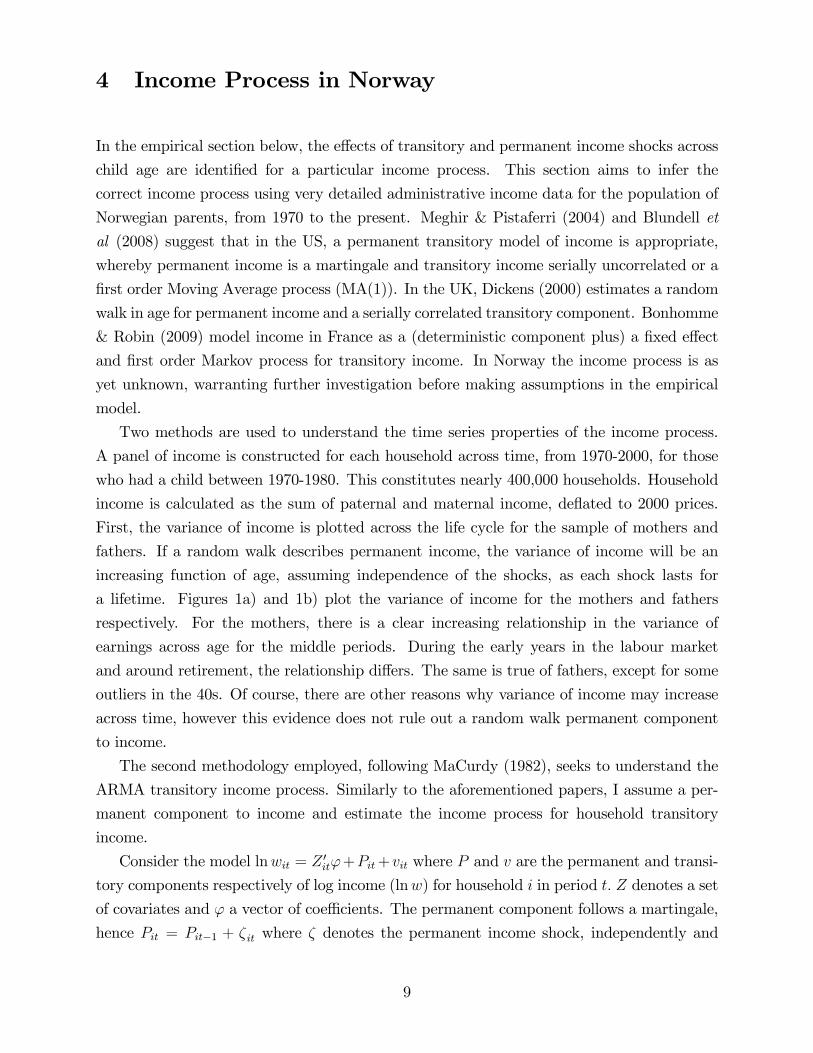
Two methods are used to understand the time series properties of the income process.

A panel of income is constructed for each household across time, from 1970-2000, for those

who had a child between 1970-1980. This constitutes nearly 400,000 households. Household

income is calculated as the sum of paternal and maternal income, de�ated to 2000 prices.

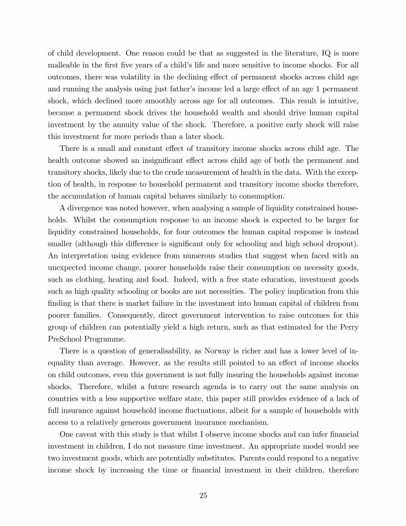
First, the variance of income is plotted across the life cycle for the sample of mothers and

fathers. If a random walk describes permanent income, the variance of income will be an

increasing function of age, assuming independence of the shocks, as each shock lasts for

a lifetime. Figures 1a) and 1b) plot the variance of income for the mothers and fathers

respectively. For the mothers, there is a clear increasing relationship in the variance of

earnings across age for the middle periods. During the early years in the labour market

and around retirement, the relationship di¤ers. The same is true of fathers, except for some

outliers in the 40s. Of course, there are other reasons why variance of income may increase

across time, however this evidence does not rule out a random walk permanent component

to income.

The second methodology employed, following MaCurdy (1982), seeks to understand the

ARMA transitory income process. Similarly to the aforementioned papers, I assume a per-

manent component to income and estimate the income process for household transitory

income.

Consider the model lnwit = Z 0it'+Pit+vit where P and v are the permanent and transi-

tory components respectively of log income (lnw) for household i in period t: Z denotes a set

of covariates and ' a vector of coe¢ cients. The permanent component follows a martingale,

hence Pit = Pit�1 + � it where � denotes the permanent income shock, independently and

9

identically distributed (iid) across i and t. This section estimates the ARMA(p; q) process

for the transitory component of income. In a general model, transitory income is given by

vit = �pXj=1

ajvit�j +

qXj=0

mj"it�j where m0 = 1: at and mt are the lag coe¢ cients and equal

zero if there is no persistence in transitory income. " denotes the transitory income shock

to the level of transitory income (v). The orders p and q of the AR and MA components are

to be established empirically.

To analyse the persistence of the transitory income component separately to the perma-

nent component, I follow MaCurdy (1982), Meghir & Pistaferri (2004) and Blundell et al

(2008) and estimate the residuals from �rst di¤erences in income� lnwit = �Z 0it'+� it+�vit;

where �xt = xt � xt�1: The order of the AR process of the �rst di¤erenced disturbances isthe same as in the levels, however �rst di¤erencing changes the order of the estimated MA

process to (q + 1) :

The �rst stage is to estimate residuals from a system of equations of �rst di¤erence log

wages in period t for household i. The controls (Z) are a quadratic in maternal and paternal

age, maternal and paternal education, marital status and municipality of residence. Results

are in column 1 of Table 2. Income growth is decreasing in the age of mothers and fathers,

at a decreasing rate and increasing in education. There is additionally a negative coe¢ cient

on marital status.

The second stage estimates autocovariances of residuals ( ) at di¤erent lags (k) from

the equation E�vtv

0t�k�= k + !t , where ! is the error in the autocovariance process and

k = f1; ::; 8g: For each lag k, the autocovariances are estimated in a system of equations

across t where the coe¢ cient on the autocovariance is constrained to be constant in each

regression. Two potential di¢ culties with estimating the autocovariances are �rstly that

the residuals are estimated in a �rst stage and secondly that there may be serial correlation

across time for households. However, MaCurdy (1981) notes that using a seemingly unrelated

regression procedure to estimate autocovariances will result in parameters and test statistics

that are asymptotically valid.

The results are reported in Table 3. The estimated autocovariances are initially negative

at one lag but fall close to zero after the �rst lag, although it remains signi�cant. Again,

between lags 2 and 3 there is another sharp drop in the autocovariances and after lag 3, they

are no longer signi�cant. This is suggestive of a low order MA process, of the order of 2 or

3 in di¤erences, or of order 1 or 2 in levels.

In conclusion, permanent income will follow a random walk and transitory income an

MA process where I will estimate the model initially for a �rst order process and test the

robustness of results to a second order process. This is the similar income process found in

10

the studies mentioned above, suggesting a similar income process in Norway as in the UK

and the US.

5 Empirical Strategy

5.1 Income Process

Log wages (lnw) for the observation i in period t are modelled as a linear function of a

permanent and a transitory component (denoted P and v respectively) and a deterministic

component of covariates (Z)

lnwit = Z0it't + Pit + vit (1)

where i = 1; ::; N and t = 1; ::; T: The unit of observation is the household-child pair.

Permanent income follows a martingale (equation 2) and transitory income is a serially

correlated MA(1) process (equation 3), where � and " denote the permanent and transitory

income shocks respectively and � the �rst order MA coe¢ cient. Section 4 provided evidence

that this is a good representation of the true income process for the sample of Norwegian

parents.

Pit = Pit�1 + � it (2)

vit = �"it�1 + "it (3)

Both permanent and transitory shocks are assumed to have a mean of zero and be

uncorrelated with each other, E (� it) = E ("it) = E (� it"it) = 0; t = 1; ::; T; i = 1; ::; N .

Following Meghir & Pistaferri (2004), de�ne y as log income with the e¤ect of the co-

variates removed in a �rst stage, yit = lnwit � Z 0it't = Pit + �"t�1 + "it: Substituting in forthe permanent income component gives

yit = Pi0 +tPs=1

� is + �"it�1 + "it (4)

Income in period t is the sum of P0; the initial level of permanent income at the start of

the child�s lifetime, representing an unobservable endowment or initial condition, past and

contemporaneous permanent income shocks and transitory shocks current and at one lag.

11

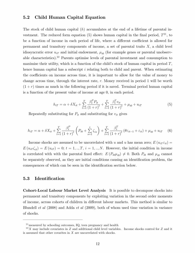
5.2 Child Human Capital Equation

The stock of child human capital (h) accumulates at the end of a lifetime of parental in-

vestment. The reduced form equation (5) shows human capital in the �nal period, T 21, to

be a function of income in each period of life, where a di¤erent coe¢ cient is allowed for

permanent and transitory components of income, a set of parental traits X; a child level

idiosyncratic error uiT and initial endowment, �i0 (for example genes or parental unobserv-

able characteristics).22 Parents optimise levels of parental investment and consumption to

maximise their utility, which is a function of the child�s stock of human capital in period T ,

hence human capital has a subscript i relating both to child and parent. When estimating

the coe¢ cients on income across time, it is important to allow for the value of money to

change across time, through the interest rate, r: Money received in period 1 will be worth

(1 + r) times as much in the following period if it is saved. Terminal period human capital

is a function of the present value of income at age 0, in each period.

hiT = �+ �Xit +TPt=1

�Pt Pit

(1 + r)t+

TPt=1

�Tt vit

(1 + r)t+ �i0 + uiT (5)

Repeatedly substituting for Pit and substituting for vit gives

hiT = �+ �Xit +TPt=1

�Pt(1 + r)t

�Pi0 +

tPs=1

� is

�+

TPt=1

�Tt(1 + r)t

(�"it�1 + "it) + �i0 + uiT (6)

Income shocks are assumed to be uncorrelated with u and u has mean zero; E (uiT "it) =

E (uiT � it) = E (uiT ) = 0; t = 1; ::; T , i = 1; ::; N . However, the initial condition in income

is correlated with with the parental �xed e¤ect: E (Pi0�i0) 6= 0: Both Pi0 and �i0 cannot

be separately observed, as they are initial conditions causing an identi�cation problem, the

consequences of which can be seen in the identi�cation section below.

5.3 Identi�cation

Cohort-Local Labour Market Level Analysis It is possible to decompose shocks into

permanent and transitory components by exploiting variation in the second order moments

of income, across cohorts of children in di¤erent labour markets. This method is similar to

Blundell et al (2008) and Adda et al (2009), both of whom used time variation in variance

of shocks.

21measured by schooling outcomes, IQ, teen pregnancy and health22X may include covariates in Z and additional child level variables. Income shocks control for Z and it

is assumed that other covarites in X are uncorrelated with shocks.

12

Meghir & Pistaferri (2004) identify the moments of the income process using information

on income alone. Given the income process above, the covariance matrix of income at

di¤erent lags is given for a cohort and labour market (c) by

cov (yit;c; yit�s;c)c = �2P0;c +t�sPl=1

�2�l;c + �2�2"t�1;c + �

2"t;c if s = 0

�2P0;c +t�sPl=1

�2�l;c + ��2"t�1 if s = 1

�2P0;c +t�sPl=1

�2�l;c if jsj > 1

(7)

where �2�t and �2"t denote the variance of permanent and transitory shocks in period t,

respectively. It is the aggregation to cohort-labour market which allows identi�cation of all

variance terms, with the exception of �2"T ; �2�T; which are not separately identi�able. For this

reason, an additional year of data is included in the period T + 1.23

The covariance matrix between income in each year of the child�s lifetime and human

capital is given below.

cov (yit;c; hiT )c =

�TPl=1

�Pl

��2P0;c +

tPs=1

�TPl=s

�Pl

��2�s;c + �

2�Tt �2"t�1

+��Tt + ��

Tt+1

��2"t + ��0P0 if t = 1

�TPl=1

�Pl

��2P0;c +

tPs=1

�TPl=s

�Pl

��2�s;c + �

��Tt�1 + ��

Tt

��2"t�1

+��Tt + ��

Tt+1

��2"t + ��0P0 if t = 2; ::; T � 1

�TPl=1

�Pl

��2P0;c +

tPs=1

�TPl=s

�Pl

��2�s;c + �

��Tt�1 + ��

Tt

��2"t�1

+�Tt �2"t + ��0P0 if t = T

(8)

where ��0P0 denotes the correlation between P0 and �0. For notational ease, the discount-

ing by interest rate r has been omitted, and coe¢ cients in equation (8) have been adjusted

to denote present values as at period 0. As noted above, the two initial conditions cannot

be separately identi�ed and consequently, the coe¢ cient on P0 will be interpreted as the

correlation between the parental initial condition and the �xed e¤ect. However, all other

parameters are identi�ed. � is estimated empirically.

Identi�cation comes from variance of shocks across cohorts and labour markets. The

23This means that �2"T+1and �2�T+1

cannot be distinguished.

13

inherent identi�cation assumption for the �rst stage is that second order moments of the

permanent and transitory income process di¤er across cohorts, labour markets and child

age, but that the e¤ect of these shocks upon child outcomes di¤ers only across child age.

Identi�cation of equation (8) relies on the estimated shocks to income being truly unexpected

by households and exogeneous. Endogeneity of income from heterogeneous life cycle pro�les

and the presence of siblings is explored in Sections 7.2 & 7.3.

Measurement error is omitted from the model to date. Meghir & Pistaferri (2004) es-

timate that between a quarter and a third of the transitory income shock variation is due

to measurement error in the Panel Study of Income Dynamics (PSID). However, the bias is

likely to be smaller in the current sample, as income is recorded from administrative data.

The variance of permanent shocks is una¤ected by the presence of measurement error.

6 Results

6.1 Income Shocks

The �rst stage of the analysis is to predict annual household income shocks, from the life

cycle pro�le of income. A regression of log household income is run upon a constant, a

quadratic in age, education, marital status and dummies for municipality of residence and

year. The �rst stage regressions, in column 2 of Table 2, show log income increasing in

parental age, but at a decreasing rate. Additionally, parent�s education and marital status

raise the household wage. The residuals estimated from these regressions indicate income

shocks in the magnitude of 0.3-1% of annual income.

The estimation of household shocks is such that all households experience an income

shock, as the annual deviation from their life cycle pro�le. Hence the incidence of an income

shock will be uncorrelated with parental traits. As the variance of the income shocks is used

for identi�cation, it is worthwhile to explore any correlation between the variance of income

shocks across a lifetime and family traits. A regression at the level of the household, of

the standard deviation of lifetime income shocks upon a quadratic in maternal and paternal

education shows that households with a low level of education have a relatively high variance

of shocks and the slope is increasing across education.24 The same pattern holds when

running the regression at the level of the labour market.

24The coe¢ cients (standard deviations) on maternal and paternal education are -0.03(0.00003) and -0.03(0.0006) and on the quadratic terms 0.001(0.00003) and 0.001(0.00003) respectively.

14

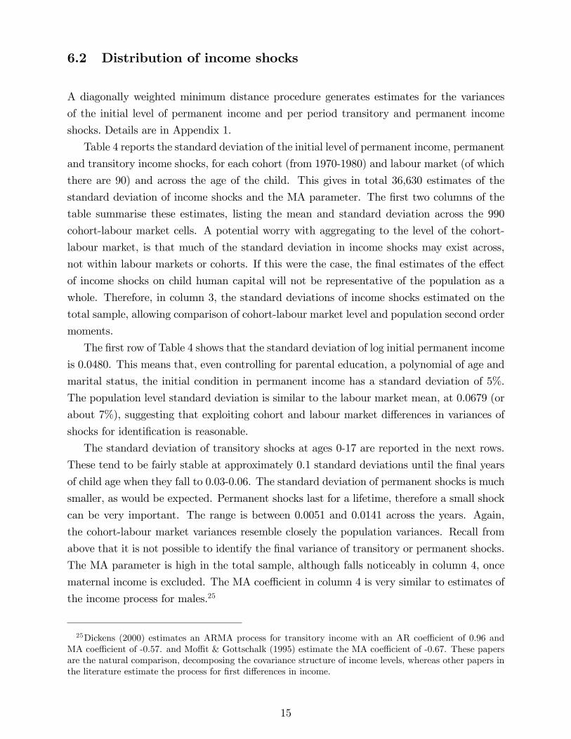
6.2 Distribution of income shocks

A diagonally weighted minimum distance procedure generates estimates for the variances

of the initial level of permanent income and per period transitory and permanent income

shocks. Details are in Appendix 1.

Table 4 reports the standard deviation of the initial level of permanent income, permanent

and transitory income shocks, for each cohort (from 1970-1980) and labour market (of which

there are 90) and across the age of the child. This gives in total 36,630 estimates of the

standard deviation of income shocks and the MA parameter. The �rst two columns of the

table summarise these estimates, listing the mean and standard deviation across the 990

cohort-labour market cells. A potential worry with aggregating to the level of the cohort-

labour market, is that much of the standard deviation in income shocks may exist across,

not within labour markets or cohorts. If this were the case, the �nal estimates of the e¤ect

of income shocks on child human capital will not be representative of the population as a

whole. Therefore, in column 3, the standard deviations of income shocks estimated on the

total sample, allowing comparison of cohort-labour market level and population second order

moments.

The �rst row of Table 4 shows that the standard deviation of log initial permanent income

is 0.0480. This means that, even controlling for parental education, a polynomial of age and

marital status, the initial condition in permanent income has a standard deviation of 5%.

The population level standard deviation is similar to the labour market mean, at 0.0679 (or

about 7%), suggesting that exploiting cohort and labour market di¤erences in variances of

shocks for identi�cation is reasonable.

The standard deviation of transitory shocks at ages 0-17 are reported in the next rows.

These tend to be fairly stable at approximately 0.1 standard deviations until the �nal years

of child age when they fall to 0.03-0.06. The standard deviation of permanent shocks is much

smaller, as would be expected. Permanent shocks last for a lifetime, therefore a small shock

can be very important. The range is between 0.0051 and 0.0141 across the years. Again,

the cohort-labour market variances resemble closely the population variances. Recall from

above that it is not possible to identify the �nal variance of transitory or permanent shocks.

The MA parameter is high in the total sample, although falls noticeably in column 4, once

maternal income is excluded. The MA coe¢ cient in column 4 is very similar to estimates of

the income process for males.25

25Dickens (2000) estimates an ARMA process for transitory income with an AR coe¢ cient of 0.96 andMA coe¢ cient of -0.57. and Mo¢ t & Gottschalk (1995) estimate the MA coe¢ cient of -0.67. These papersare the natural comparison, decomposing the covariance structure of income levels, whereas other papers inthe literature estimate the process for �rst di¤erences in income.

15

6.3 E¤ect of shocks on adolescent outcomes

An innovative aspect of this paper is estimation of the e¤ect of the household permanent

and transitory income shocks upon child outcomes. This section documents the results,

examining whether the realisation of transitory and permanent income shocks will have a

heterogeneous e¤ect upon child outcomes, depending upon the age of the child at realisation.

The variances of transitory and permanent income shocks across child age are applied to

equation (8) to estimate the e¤ect of the income shocks upon child human capital outcomes.

The human capital equation (6) allows the e¤ect of income shocks to vary across child

age. Before estimating this complex model, it is interesting to restrict the coe¢ cients to be

homogeneous across child age, estimating the following function

hiT = �0 + �1Pi0 + �2� it + �3"it + �i0 + uiT ; t = 1; ::; 16:

A panel data is constructed at the cohort - labour market - child age level. Regression

results are reported in Table 5. There are15840 observations (90 labour markets, 11 cohorts,

for ages 1-16).26 Two di¤erent functional forms are estimated. In columns 1, 3, 5, 7 & 9, the

human capital outcomes are estimated as a linear function of the initial level of permanent

income (P0), a transitory income shock and a permanent income shock. Columns 2, 4, 6,

8 & 10 include an interaction term of permanent (transitory) shocks with child age thus

allowing some heterogeneity in the e¤ect of income shocks across child age. The variable

high school dropout has been rede�ned, to indicate completion of high school, to enable ease

of comparison with the other outcomes.

The estimates are standardised so that both the income shocks and the outcomes are

expressed in terms of a standard deviation. Put another way, the coe¢ cient represents the

standard deviation change in the outcome from a standard deviation change in the income

shock.

Starting with the �rst outcome in column 1, a change in P0 by a standard deviation

(5%) is correlated with an increase in completed years of child schooling by 1.177 standard

deviations. Columns 3, 5, 7 & 9 show that there is a strong and signi�cant e¤ect of P0

for all other outcomes, except health. This e¤ect is similar regardless of the speci�cation of

transitory and permanent income shocks. Raising P0 by 5% is correlated with higher values

of years of schooling, probability of completing out of high school, college attendance, IQ

and health by up to 1.193, 0.206, 0.156, 0.763, and 0.171 standard deviations respectively.

This indicates a strong correlate between family background and child outcomes.

The �rst column of data for each outcome shows that transitory income shocks improve

child human capital (columns 1, 3, 5, 7 & 9), however once the interaction between transi-

26It is not possible to distinguish transitory and permanent shocks at age 17.

16

tory shocks and child age is added, the level e¤ect becomes negative or insigni�cant. The

interaction between transitory income shock and child age is positive - initially there is a

negative e¤ect of transitory shocks which is increasing across child age. Permanent shocks

have a larger e¤ect on education, high school dropout and IQ, as would be expected from

the PIH. The interaction between permanent shocks and child age is insigni�cant.

Next, the fully �exible model is estimated from equation (8) and the age speci�c coef-

�cients on the permanent and transitory income shocks and initial permanent income are

reported in Table 6a and 6b. Again, the coe¢ cients report the e¤ect of a standard deviation

change in the speci�c income shock, upon the standard deviation change in human capital.

The results of the e¤ect of permanent and transitory shocks across child age are easier to

see in graphical form hence additionally, Figures 2a-2j plot the coe¢ cients across age, again

in standard deviations of the child outcome.

Initial Condition in Income Examining �rst how the initial condition in income

drives child human capital outcomes, in row 1 from Tables 6a and 6b the log initial level of

permanent income (reported as age 0, permanent) has a strong and signi�cant value. This

picks up the correlation between family background and child achievement. For years of

schooling, the coe¢ cient is 0.3795, meaning that a standard deviation increase in the initial

condition is correlated with higher schooling by 0.38 standard deviations, equivalent to 0.93

years of schooling. For the other outcomes, a standard deviation increase in P0 is correlated

with an increase in the probability of dropping out of high school, college attendance, IQ

and health by 0.2668, 0.3494, 0.2895 and 0.0230 standard deviations respectively (equivalent

to an increase of 11%, 17.1%, 0.52 points and 0.04 points for dropout, college, IQ and health

respectively). The smallest correlate is on the health outcome. As health is measured on a

9 point scale, with a very large majority of participants receiving the top score of 9, it is not

surprising that the measure is not highly correlated with the initial condition. The strong

correlation between the initial condition and the parental �xed e¤ect indicates signi�cant

dispersion in outcomes by family background at birth in Norway.

Permanent Income Shocks Figures 2a, c, e, g & i plot the coe¢ cients on permanent

income shocks realised in every year of the child�s lifetime, upon the range of child outcomes.

These relate to the columns labelled "Permanent" for ages 1-16 in Tables 6a and 6b.

A standard deviation increase in the permanent shock at age 1 raises schooling by 0.0866

standard deviations. This transmission falls initially across child age, albeit nosily, such that

a shock at age 16 has a smaller e¤ect than at age 1, raising schooling by only 0.0019 standard

deviations. The larger e¤ect of the permanent shock realised during early years is intuitive,

17

given that the early permanent shock shifts household wealth forever and therefore drive

income realisations for all future periods.

A very similar pattern between the transmission e¤ect of permanent income shocks re-

alised across child age, upon the probability of completing high school and college completion,

is observed in Figure 2c and 2e respectively. The e¤ect is large at age 1 (a 1 standard devia-

tion increase in the shock raises the probability of completing high school (college attendance)

by 0.0599 (0.0659) standard deviations) and the transmission e¤ect declines across child age

such that a 1 standard deviation shock at age 16 raises the probability of competing high

school (college) by 0.0094 (-0.0077) standard deviations. Again the decline is noisy, with

jumps in the e¤ect around ages 2, 6, 9 and 15.

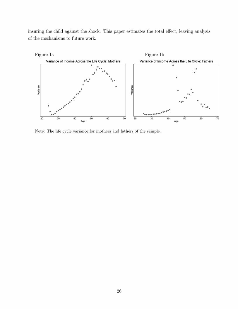
For the outcome IQ in Figure 2g (for males only), the e¤ect of permanent income shocks

between ages 1-8 is relatively �at, with a decreasing slope from age 9-16. A pure permanent

income e¤ect would lead to a declining curve, but for early years the return to income shocks

remains high. One interpretation is that the e¤ect does not fall in early years because as

Cunha & Heckman (2007, 2008) suggest, cognitive ability is more malleable in early years

and therefore more sensitive to parental income shocks.

Figure 2i shows that there is a noisy transmission e¤ect of permanent shocks upon health,

with the coe¢ cients all insigni�cantly di¤erent to zero. It cannot be ruled out that the noisy

pattern is due to the poor measurement of health as 85% of the boys achieved the highest

score of physical health.

A permanent income shock realised when the child is age 1 is realised in all future

income and therefore the declining e¤ect of the shock across child age is intuitive. It changes

household wealth for all future periods and therefore has a larger e¤ect upon child outcomes.

Thus, the transmission e¤ect of permanent shocks to child human capital behave similarly

as the e¤ect of consumption.

However the decline across child age is noisy. There tends to be a jump in the year after

birth, at ages 6, 9 and 15. These jumps may coincide with maternal labour supply. For

example, permanent income would increase if mothers go back to work after having a child.

This raises the question of whether the shocks as estimated in this paper, are truly shocks,

or anticipated by the households themselves. If the shock just picks up an expected change

in labour supply, then the resulting change in child outcomes (through adjusted parental

investment) would not be as the model predicted. One way to overcome this problem would

be to run the analysis solely on paternal income, which �uctuates less around maternity

leave and child schooling. These results are reported in the following section.

18

Transitory Income Shocks Turning now to the transmission between transitory in-

come shocks and child human capital, Figure 2b, d, f, h, & j plot the estimates of the e¤ect

of transitory income shocks for ages 1-16. Again, the coe¢ cients and standard errors have

been adjusted for the standard deviation of the transitory income shocks at each child age.

The columns labelled "Transitory" in Tables 6a and 6b report the coe¢ cients and standard

errors. There is a relatively constant e¤ect of transitory income shocks across child age

and the magnitude of the e¤ect is lower than for permanent shocks. A standard deviation

shock increase at age 1 and age 16 raises schooling by 0.0327 and 0.0378 standard deviations

respectively. Again the e¤ect on health is instatistically di¤erent to zero.

To summarise, there is a large coe¢ cient on the initial level of permanent income, or

parental �xed e¤ect, suggesting signi�cant heterogeneity in child outcomes which is deter-

mined at the birth of the child. This is interesting, as often Norway is considered a very

equal country, with a compressed income distribution. However, the evidence suggests large

variance in outcomes driven by a family initial condition.

Two �ndings, that the transmission of transitory shocks to outcomes is constant across

age, and of a lower magnitude than permanent shocks, are consistent with the PIH. The

annuity value of a permanent income shock at age 1 is greater than for a transitory shock.

Interestingly, the coe¢ cients of the permanent and transitory income shocks converge

towards the �nal period. This is consistent with the idea that a permanent shock in the

�nal period of human capital investment should drive human capital to a similar degree as

a transitory income shock in that period. Moving towards the terminal period of human

capital accumulation, the annuity value of the permanent and transitory shock aligns and

so therefore does the e¤ect of the shocks.

6.4 Paternal Income

The above analysis is repeated using paternal income shocks rather than shocks to the

sum of maternal and paternal income. The e¤ect of a household permanent income shock

declines noisily across child age. These jumps may coincide with a change in maternal labour

supply which shifts permanent income. For example, the age 2 jump could re�ect ending

maternity leave and at age 7 the children started school, freeing up the mothers to enter the

labour market. This section estimates the e¤ect of paternal income shocks, excluding any

contribution from maternal income. This method does not remove the endogeneous decision

of mothers to enter the labour market, as this decision is made jointly with paternal labour

supply. However, paternal labour supply is arguably less sensitive to such changes across the

child life cycle

19

Estimated standard deviations of the shocks are reported in Column 4 of Table 4. The

variances are slightly higher than for the total sample.

Figures 3a-3e plot the e¤ect of permanent shocks to both household and paternal in-

come upon child outcomes, across child age. As the variance of income shocks di¤er across

household income and paternal income, the coe¢ cient represents the e¤ect of a standard

deviation change in household income shock.27 Indeed, the �gures show that when only

paternal income is considered, the e¤ect of permanent income shocks falls more smoothly

from the age of 1 to 16 than was observed for household income. The paternal permanent

income e¤ect lies slightly below the household e¤ect for early years, however the di¤erence

is insigni�cant.28

6.5 Liquidity Constrained Sample

If parents face binding liquidity constraints, they will be unable to borrow and save in order

to smooth transitory income shocks. Consequently, the e¤ect of transitory shocks will be

larger for a liquidity constrained sample. It is interesting to see whether the accumulation of

child human capital of liquidity constrained parents responds similarly to consumption, by

repeating the above analysis on a group of poor parents, most likely to face credit constraints.

To do so, I de�ne a household to be liquidity constrained if their permanent income is in the

second decile or below.29 Permanent income is de�ned as the sum of real income when the

child is aged 0-18.

The standard deviations of shocks for the liquidity constrained sample are reported in

Column 5 of Table 4. The standard deviation in the initial condition is lower, as this is

a more homogeneous group in terms of income. Variances of the shocks are slightly larger

than in the total sample. Again, to compare the e¤ect of transitory income shocks for the

liquidity constrained sample, normalisation is by the total sample variance.

Results are in Figures 4a-4e which plot the coe¢ cients for the total sample and for the

liquidity constrained (or "constrained") sample. What is instantly obvious from the �gures

is that, for four outcomes - years of schooling, high school dropout, college attendance

and IQ - the e¤ect of the transitory income shocks is larger in magnitude than for the

liquidity constrained sample, although this di¤erence is insigni�cant for the latter outcomes.

The higher e¤ect is contrary to expectations and suggests that human capital accumulation

behaves di¤erently to consumption, for liquidity constrained households. To give an example,

27The results are not signi�cantly changed by this normalisation.28There is no statistical di¤erence in the e¤ect of transitory shocks to paternal income compared to

household shocks.29Following Souleles (1999).

20

the e¤ect of a 1 standard deviation increase in transitory income shock at ages 1 and 16 upon

years of schooling, is around 0.0327 and 0.0378 standard deviations for the total sample, but

is 0.0187 and 0.0168 for the liquidity constrained sample. For the health outcome the e¤ect

is again instatistically di¤erent to zero.30

One interpretation is that when faced with an unexpected change in income, poor house-

holds do raise their consumption by a larger proportion than a household in which a liquidity

constraint does not bind. However, the types of goods purchased may be di¤erent. Attana-

sio et al (2005) analyse the expenditure patterns of parents in receipt of a cash transfer,

conditional upon their child�s attendance school, in the Familias en Accion programme in

Colombia. They �nd parents use the additional funds to raise consumption of protein rich

food and child clothing. Surprisingly, similar �ndings emerge from studies in more developed

countries. Gregg et al (2006) found that the result of numerous government policies to raise

household income was to enable poor families to catch up their richer counterparts, in terms

of clothing and housing costs. Indeed, a report by Farrell & O�Connor (2003) interviewed

37 households receiving the UK Working Family Tax Credit and additionally a survey by

Romich & Weisner (2000) on a sample of household receiving the Earned Income Tax Credit

in the US, found that recipients spend the additional money on household food consumption

and heating homes - necessity goods. As described above, a mechanism through which in-

come shocks are transferred into child human capital is through parental investment. Most

developed (and even developing) countries o¤er a free state education. Therefore, in receipt

of an unexpected change in income, the evidence suggests that these poorer household do not

raise investment on books and private tuition for their children, as they are not necessities,

but rather heat the house, buy clothes and food. This would explain why a shock to income

raises schooling outcomes to a lesser extent for poor households than for rich households. Of

course, feeding children can also be seen as investment in children and the income shocks

have statistically similar e¤ects on IQ in the constrained and the non-constrained house-

holds. This interpretation is observationally equivalent to the idea that poorer parents have

lower tastes for education.

This �nding warrants further research, as there are other explanations which include

that the welfare state in Norway insures poor families against income shocks or that poorer

households have higher discount rates. It is however unclear why these mechanisms would

insure all outcomes except for IQ, as for this outcome there was homogeneity in the e¤ect

of both permanent and transitory income shocks for the poor households as for the total

sample.

30Permanent income shocks have a smaller magnitude between ages 0-4 and 12-16 in the liquidity con-strained sample for the outcomes years of schooling, dropout, college and IQ, but no di¤erence for health.

21

The �nding that the stock of adolescent or adult human capital responds less to income

shocks for liquidity constrained parents is consistent with existing literature which �nd high

returns from interventions which raise investments in child human capital. For example,

Heckman et al (2009) �nd returns of 7-10% from the Perry Preschool Programme, which

provided quite intensive treatment for a randomly selected group of disadvantaged African

American families. Such a high return could be interpreted to indicate that this group of

families are not optimally investing in the human capital of their children. An alternative

explanation is that poorer families cannot prioritise investment in child human capital, but

rather choose to consume necessity goods. Hence, they are optimising but subject to binding

constraints and consequently direct intervention to raise the human capital of children can

be very e¤ective.

7 Robustness Checks

A structural model for income generates the results presented above. Section 4 ascertained

the correct income process for the sample of parents in Norway, as an MA(1) or MA(2)

process for transitory income. This was well identi�ed from a panel of around 400,000

families across 30 years. As a robustness check the e¤ect on results from changing to the

income process to an MA(2) in transitory income is analysed in Section 7.1. Sections 7.2

and 7.3 explore the endogeneity of family income, by life cycle pro�les of income and the

presence of siblings.

7.1 Assuming MA(2) Process for Transitory Income

Section 4 estimated a process for transitory income that was described by an MA(1) or an

MA(2). This section tests the sensitivity of the e¤ect of permanent and transitory income

upon child human capital to the order of the MA process, by extending to a second order

process. That is, vit = "it + �1"it�1 + �2"it�2:

For all outcomes, the results are not statistically di¤erent with the two processes for

transitory income. The results of the paper are robust to a substantial change in the assumed

income process used to decompose shocks into permanent and transitory components.

7.2 Are the shocks unexpected?

The methodology assumes that permanent income shocks are not foreseeable by families.

It may be however that �uctuations in income which seem to an econometrician to be a

permanent shock were in fact predictable. If parents expected an increase (decrease) in their

22

permanent income in the future, the families may raise (lower) contemporaneous investment

in child human capital. Consequently the response of human capital to the realised change

in permanent income will be subdued and the estimated e¤ect of the true permanent shock

prone to a downward bias.

It is not possible to directly test whether changes in income which are de�ned as unex-

pected accord with true expectations. However, it is possible to understand under which

conditions the misclassi�cation of income changes would generate the results in the main

paper and subsequently test the sensitivity of these results to a change in these conditions.

Take a family which expects an upwards sloping life cycle pro�le of permanent income

conditional on age, education and marital status.31 The PIH predicts that ceteris paribus,

this family would borrow early in life and save later in life to optimally smooth investment in

child human capital. Interpreting these changes in permanent income as unexpected would

lead human capital to seemingly "over-respond" to early low income and "under-react"

to later high income. This example would generate exactly the downward sloping pro�le

estimated for the e¤ect of permanent income shocks across child age.

Using the panel on household income I am able to categorise parents into di¤erent life

cycle pro�les and analyse the heterogeneity in the e¤ect of permanent income shocks across

groups. If the above results for the e¤ect of permanent income hold for households with non-

increasing life cycle pro�les, it will be indicative that the methodology does not misclassify

foreseeable permanent income �uctuations as unexpected.

Using a randomly selected sample of 40% of households, I run regressions of log household

income on the age of the child and the age squared. From the coe¢ cients, I categorise

the income pro�le of each observation (of a parent-child pair) into an increasing pro�le,

decreasing, inverse u-shaped and u-shaped. Then, I repeat the estimation from the bulk of

the paper, on the sample of households with an increasing life cycle pro�le and all other

households.

The �rst point to note is that only 12.37% of households have an increasing life cycle

pro�le, meaning that these are unlikely to be driving the result that permanent income has

a declining e¤ect across child age. For the other households, 1.23%, 64.16% and 22.23% of

households were categorised as having decreasing, inverse-u and u-shaped pro�les respec-

tively.32

Results, available upon request, show that for households with a non-increasing pro�le,

there is no statistical di¤erence in the relationship between permanent income shocks and

31They may expect a promotion in the following year or know of planned cuts to wage increases.32This does not require the pro�les to be signi�cant. If the restriction is added that the pro�les are

signi�cant, the sample sizes change to 16.23%, 0.52%, 34.70% and 9.15% with the remaining householdshaving a �at pro�le across age.

23

child outcomes as in the total sample. The results are robust to the life cycle pro�le and

therefore to the test of the assumption that shocks are unexpected.

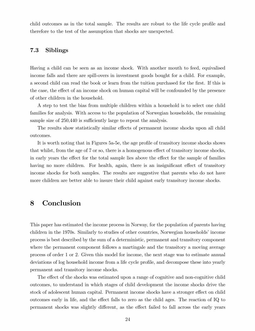
7.3 Siblings

Having a child can be seen as an income shock. With another mouth to feed, equivalised

income falls and there are spill-overs in investment goods bought for a child. For example,

a second child can read the book or learn from the tuition purchased for the �rst. If this is

the case, the e¤ect of an income shock on human capital will be confounded by the presence

of other children in the household.

A step to test the bias from multiple children within a household is to select one child

families for analysis. With access to the population of Norwegian households, the remaining

sample size of 250,440 is su¢ ciently large to repeat the analysis.

The results show statistically similar e¤ects of permanent income shocks upon all child

outcomes.

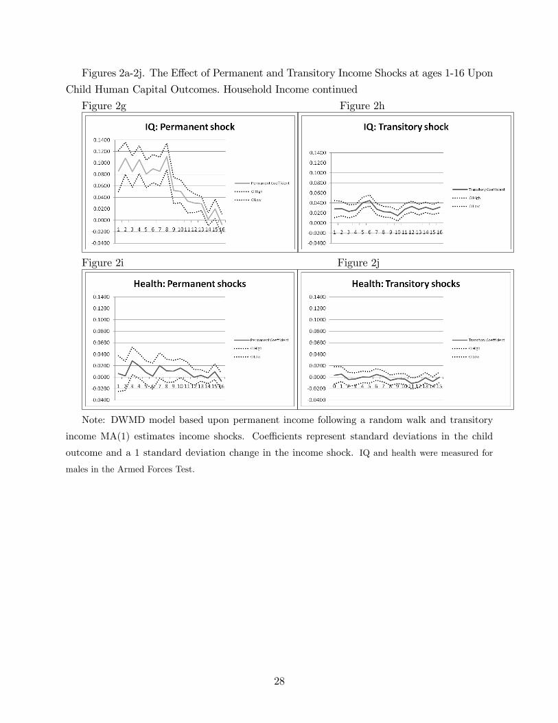
It is worth noting that in Figures 5a-5e, the age pro�le of transitory income shocks shows

that whilst, from the age of 7 or so, there is a homogenous e¤ect of transitory income shocks,

in early years the e¤ect for the total sample lies above the e¤ect for the sample of families

having no more children. For health, again, there is an insigni�cant e¤ect of transitory

income shocks for both samples. The results are suggestive that parents who do not have

more children are better able to insure their child against early transitory income shocks.

8 Conclusion

This paper has estimated the income process in Norway, for the population of parents having

children in the 1970s. Similarly to studies of other countries, Norwegian households�income

process is best described by the sum of a deterministic, permanent and transitory component

where the permanent component follows a martingale and the transitory a moving average

process of order 1 or 2. Given this model for income, the next stage was to estimate annual

deviations of log household income from a life cycle pro�le, and decompose these into yearly

permanent and transitory income shocks.

The e¤ect of the shocks was estimated upon a range of cognitive and non-cognitive child

outcomes, to understand in which stages of child development the income shocks drive the

stock of adolescent human capital. Permanent income shocks have a stronger e¤ect on child

outcomes early in life, and the e¤ect falls to zero as the child ages. The reaction of IQ to

permanent shocks was slightly di¤erent, as the e¤ect failed to fall across the early years

24

of child development. One reason could be that as suggested in the literature, IQ is more

malleable in the �rst �ve years of a child�s life and more sensitive to income shocks. For all

outcomes, there was volatility in the declining e¤ect of permanent shocks across child age

and running the analysis using just father�s income led a large e¤ect of an age 1 permanent

shock, which declined more smoothly across age for all outcomes. This result is intuitive,

because a permanent shock drives the household wealth and should drive human capital

investment by the annuity value of the shock. Therefore, a positive early shock will raise

this investment for more periods than a later shock.

There is a small and constant e¤ect of transitory income shocks across child age. The

health outcome showed an insigni�cant e¤ect across child age of both the permanent and

transitory shocks, likely due to the crude measurement of health in the data. With the excep-

tion of health, in response to household permanent and transitory income shocks therefore,

the accumulation of human capital behaves similarly to consumption.

A divergence was noted however, when analysing a sample of liquidity constrained house-

holds. Whilst the consumption response to an income shock is expected to be larger for

liquidity constrained households, for four outcomes the human capital response is instead

smaller (although this di¤erence is signi�cant only for schooling and high school dropout).

An interpretation using evidence from numerous studies that suggest when faced with an

unexpected income change, poorer households raise their consumption on necessity goods,

such as clothing, heating and food. Indeed, with a free state education, investment goods

such as high quality schooling or books are not necessities. The policy implication from this

�nding is that there is market failure in the investment into human capital of children from

poorer families. Consequently, direct government intervention to raise outcomes for this

group of children can potentially yield a high return, such as that estimated for the Perry

PreSchool Programme.

There is a question of generalisability, as Norway is richer and has a lower level of in-

equality than average. However, as the results still pointed to an e¤ect of income shocks

on child outcomes, even this government is not fully insuring the households against income

shocks. Therefore, whilst a future research agenda is to carry out the same analysis on

countries with a less supportive welfare state, this paper still provides evidence of a lack of

full insurance against household income �uctuations, albeit for a sample of households with

access to a relatively generous government insurance mechanism.

One caveat with this study is that whilst I observe income shocks and can infer �nancial

investment in children, I do not measure time investment. An appropriate model would see

two investment goods, which are potentially substitutes. Parents could respond to a negative

income shock by increasing the time or �nancial investment in their children, therefore

25

insuring the child against the shock. This paper estimates the total e¤ect, leaving analysis

of the mechanisms to future work.

Figure 1a Figure 1b

Note: The life cycle variance for mothers and fathers of the sample.

26

Figures 2a-2j. The E¤ect of Permanent and Transitory Income Shocks at ages 1-16 Upon

Child Human Capital Outcomes. Household Income.

Figure 2a Figure 2b

Figure 2c Figure 2d

Figure 2e Figure 2f

Note: DWMD model based upon permanent income following a random walk and transitory

income MA(1) estimates income shocks. Coe¢ cients represent standard deviations in the child

outcome and a 1 standard deviation change in the income shock. Education denotes years of schooling,

dropout indicates not leaving school at the compulsory age and college attendance at college/university.

27

Figures 2a-2j. The E¤ect of Permanent and Transitory Income Shocks at ages 1-16 Upon

Child Human Capital Outcomes. Household Income continued

Figure 2g Figure 2h

Figure 2i Figure 2j

Note: DWMD model based upon permanent income following a random walk and transitory

income MA(1) estimates income shocks. Coe¢ cients represent standard deviations in the child

outcome and a 1 standard deviation change in the income shock. IQ and health were measured for

males in the Armed Forces Test.

28

Figures 3a-3e. The E¤ect of Permanent Income Shocks at ages 1-16 Upon Child Human

Capital Outcomes. Paternal and Household Income.

Figure 3a Figure 3b

Figure 3c Figure 3d

Figure 3e

Note: DWMD model based upon permanent income following a random walk and transitory

income MA(1) estimates income shocks. Coe¢ cients represent standard deviations in the child

outcome and a 1 standard deviation change in the income shock.

29

Figures 4a-4e. The E¤ect of Transitory Income Shocks at ages 1-16 Upon Child Human

Capital Outcomes. Liquidity Constrained and Total Samples.

Figure 4a Figure 4b

Figure 4c Figure 4d

Figure 4e

Note:DWMD model based upon permanent income following a random walk and transitory

income MA(1) estimates income shocks. Coe¢ cients represent standard deviations in the child

outcome and a 1 standard deviation change in the income shock. Liquidity constrained sample:

permanent income in decile 2 or below.

30

Figures 5a-5e. The E¤ect of Transitory Income Shocks at ages 1-16 Upon Child Human

Capital Outcomes. Total Sample and Single Child Sample

Figure 5a Figure 5b

Figure 5c Figure 5d

Figure 5e

Note: Single children sample includes 250,440 children. DWMD model based upon permanent

income following a random walk and transitory income MA(1) estimates income shocks. Coe¢ cients

represent standard deviations in the child outcome and a 1 standard deviation change in the income

shock.

31

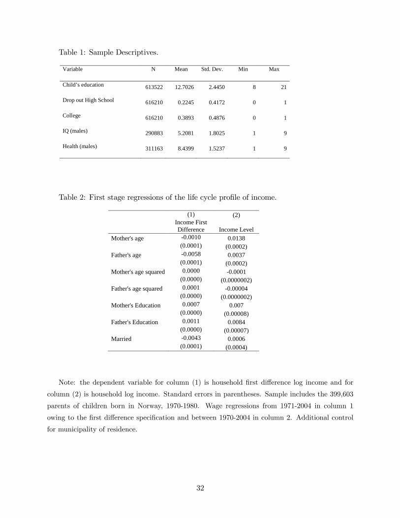
Table 1: Sample Descriptives.

Variable N Mean Std. Dev. Min Max

Child’s education 613522 12.7026 2.4450 8 21

Drop out High School 616210 0.2245 0.4172 0 1

College 616210 0.3893 0.4876 0 1

IQ (males) 290883 5.2081 1.8025 1 9

Health (males) 311163 8.4399 1.5237 1 9

Table 2: First stage regressions of the life cycle pro�le of income.

(1) (2)Income FirstDifference Income Level

Mother's age ­0.0010 0.0138(0.0001) (0.0002)

Father's age ­0.0058 0.0037(0.0001) (0.0002)

Mother's age squared 0.0000 ­0.0001(0.0000) (0.0000002)

Father's age squared 0.0001 ­0.00004(0.0000) (0.0000002)

Mother's Education 0.0007 0.007(0.0000) (0.00008)

Father's Education 0.0011 0.0084(0.0000) (0.00007)

Married ­0.0043 0.0006(0.0001) (0.0004)

Note: the dependent variable for column (1) is household �rst di¤erence log income and for

column (2) is household log income. Standard errors in parentheses. Sample includes the 399,603

parents of children born in Norway, 1970-1980. Wage regressions from 1971-2004 in column 1

owing to the �rst di¤erence speci�cation and between 1970-2004 in column 2. Additional control

for municipality of residence.

32

Ta ble3:Autocovariancesofresidualsfrom

logincomedi¤erences�lnwit��Z0 it�:

Lag

k=0

k=1

k=2

k=3

k=4

k=5

k=6

k=7

k=8

Aut

ocov

aria

nce

0.06

10**

­0.0

145*

*­0

.004

1**

­0.0

028*

*­0

.000

9­0

.001

1­0

.000

1­0

.000

50.

0012

Stan

dard

 err

or(0

.004

4)(0

.001

8)(0

.001

2)(0

.001

0)(0

.001

1)(0

.001

0)(0

.001

0)(0

.001

1)(0

.000

9)

Note:Theresidualsareestimatedfrom

aregressionoflogincomeonpaternalage,education,educationsquared,maritalstatusand

dummyvariablesformunicipalityofresidence.Eachcolumnrepresentsaregressionforeachlag,estimatedinasystem

ofequations

acrosst.Autocovariancesrestrictedtobehomogeneousacrossyears.N=399,603households,between1971-2000.

33

ISSN 2045-6557

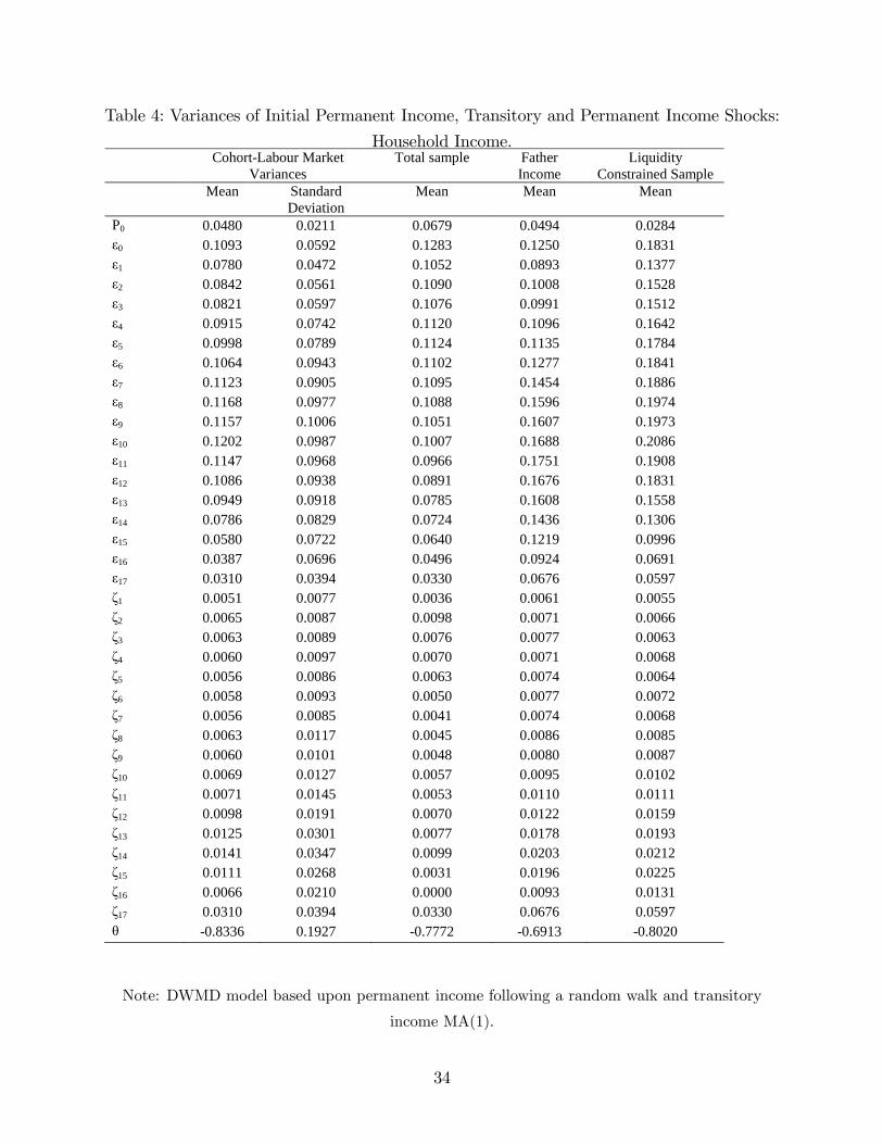
Table 4: Variances of Initial Permanent Income, Transitory and Permanent Income Shocks:

Household Income.Cohort­Labour Market

VariancesTotal sample Father

IncomeLiquidity

Constrained SampleMean Standard

DeviationMean Mean Mean

P0 0.0480 0.0211 0.0679 0.0494 0.0284ε0 0.1093 0.0592 0.1283 0.1250 0.1831ε1 0.0780 0.0472 0.1052 0.0893 0.1377ε2 0.0842 0.0561 0.1090 0.1008 0.1528ε3 0.0821 0.0597 0.1076 0.0991 0.1512ε4 0.0915 0.0742 0.1120 0.1096 0.1642ε5 0.0998 0.0789 0.1124 0.1135 0.1784ε6 0.1064 0.0943 0.1102 0.1277 0.1841ε7 0.1123 0.0905 0.1095 0.1454 0.1886ε8 0.1168 0.0977 0.1088 0.1596 0.1974ε9 0.1157 0.1006 0.1051 0.1607 0.1973ε10 0.1202 0.0987 0.1007 0.1688 0.2086ε11 0.1147 0.0968 0.0966 0.1751 0.1908ε12 0.1086 0.0938 0.0891 0.1676 0.1831ε13 0.0949 0.0918 0.0785 0.1608 0.1558ε14 0.0786 0.0829 0.0724 0.1436 0.1306ε15 0.0580 0.0722 0.0640 0.1219 0.0996ε16 0.0387 0.0696 0.0496 0.0924 0.0691ε17 0.0310 0.0394 0.0330 0.0676 0.0597ζ1 0.0051 0.0077 0.0036 0.0061 0.0055ζ2 0.0065 0.0087 0.0098 0.0071 0.0066ζ3 0.0063 0.0089 0.0076 0.0077 0.0063ζ4 0.0060 0.0097 0.0070 0.0071 0.0068ζ5 0.0056 0.0086 0.0063 0.0074 0.0064ζ6 0.0058 0.0093 0.0050 0.0077 0.0072ζ7 0.0056 0.0085 0.0041 0.0074 0.0068ζ8 0.0063 0.0117 0.0045 0.0086 0.0085ζ9 0.0060 0.0101 0.0048 0.0080 0.0087ζ10 0.0069 0.0127 0.0057 0.0095 0.0102ζ11 0.0071 0.0145 0.0053 0.0110 0.0111ζ12 0.0098 0.0191 0.0070 0.0122 0.0159ζ13 0.0125 0.0301 0.0077 0.0178 0.0193ζ14 0.0141 0.0347 0.0099 0.0203 0.0212ζ15 0.0111 0.0268 0.0031 0.0196 0.0225ζ16 0.0066 0.0210 0.0000 0.0093 0.0131ζ17 0.0310 0.0394 0.0330 0.0676 0.0597θ ­0.8336 0.1927 ­0.7772 ­0.6913 ­0.8020

Note: DWMD model based upon permanent income following a random walk and transitory

income MA(1).

34

Ta ble5:TheE¤ectofTheTimingofHouseholdTransitoryShocks,InitialPermanentIncome(P0)andPermanentShocks

uponChildOutcomes:WithRestrictionsonCoe¢cientsAcrossChildAge.

Educ

atio

nCo

mpl

ete H

igh 

Scho

olU

nive

rsity

/Col

lege

IQH

ealth

(1)

(2)

(3)

(4)

(5)

(6)

(7)

(8)

(9)

(10)

P01.

177*

**1.

193*

**0.

204*

**0.

206*

**0.

153*

**0.

156*

**0.

754*

**0.

763*

**0.

170

0.17

1(0

.152

)(0

.151

)(0

.021

)(0

.021

)(0

.035

)(0

.034

)(0

.145

)(0

.146

)(0

.103

)(0

.103

)Tr

ansit

ory

0.30

4***

­0.1

20**

0.04

8***

­0.0

110.

055*

**­0

.023

***

0.18

1***

­0.0

88**

0.03

0­0

.036

(0.0

28)

(0.0

47)

(0.0

06)

(0.0

11)

(0.0

06)

(0.0

08)

(0.0

25)

(0.0

44)

(0.0

23)

(0.0

27)

Tran

sitor

y*ag

e0.

047*

**0.

007*

**0.

009*

**0.

030*

**0.

007*

**(0

.004

)(0

.001

)(0

.001

)(0

.004

)(0

.002

)Pe

rman

ent

0.40

8***

0.13

20.

068*

**0.

048

0.02

7**

­0.0

340.

240*

**0.

447*

0.02

20.

373*

*(0

.055

)(0

.253

)(0

.013

)(0

.044

)(0

.011

)(0

.048

)(0

.082

)(0

.258

)(0

.056

)(0

.182

)Pe

rman

ent

*age

0.00

8­0

.000

0.00

2­0

.025

­0.0

30**

(0.0

20)

(0.0

04)

(0.0

04)

(0.0

21)

(0.0

13)

N15

,840

15,8

4015

,840

15,8

4015

,840

15,8

4015

,840

15,8

4015

,840

15,8

40

Note:N=90labourmarkets,11cohorts,16yearsofchild

age.Standarderrorsinparentheses.Dependentvariableshavebeen

standardisedsuchthatthecoe¢cientsareexpressedinstandarddeviationsoftheoutcomes.Thecoe¢cientsontransitory(permanent)

incomeshocksarerestrictedtobeconstantacrosschildageinthe�rstspeci�cation,andincludeanadditionalterm

oftheinteraction

betweentheshockandchildageinthesecond.

35

ISSN 2045-6557

Table 6a: The E¤ect of The Timing of Transitory Shocks, Initial Permanent Income (Pe-

riod 0) and Permanent Shocks upon Child Outcomes: Without Restrictions on Coe¢ cients

Across Child Age. Household Income.

Education High School CollegeChild Age Permanent Transitory Permanent Transitory Permanent Transitory

0 0.3795 0.2668 0.3494(0.0085) (0.0080) (0.0086)

1 0.0866 0.0327 0.0599 0.0364 0.0659 0.0234(0.0141) (0.0060) (0.0126) (0.0061) (0.0141) (0.0061)

2 0.1116 0.0320 0.0892 0.0340 0.1056 0.0243(0.0107) (0.0050) (0.0106) (0.0051) (0.0108) (0.0051)

3 0.0712 0.0407 0.0568 0.0328 0.0649 0.0360(0.0097) (0.0047) (0.0099) (0.0048) (0.0099) (0.0047)

4 0.0659 0.0375 0.0517 0.0283 0.0726 0.0353(0.0089) (0.0041) (0.0088) (0.0042) (0.0091) (0.0041)

5 0.0668 0.0494 0.0554 0.0432 0.0715 0.0408(0.0086) (0.0038) (0.0088) (0.0040) (0.0087) (0.0039)

6 0.0980 0.0426 0.0774 0.0320 0.0975 0.0435(0.0089) (0.0039) (0.0091) (0.0040) (0.0090) (0.0039)

7 0.0705 0.0441 0.0629 0.0299 0.0755 0.0408(0.0091) (0.0038) (0.0089) (0.0039) (0.0093) (0.0037)

8 0.0653 0.0567 0.0534 0.0398 0.0591 0.0481(0.0088) (0.0038) (0.0087) (0.0039) (0.0088) (0.0037)

9 0.0879 0.0503 0.0688 0.0323 0.0765 0.0504(0.0085) (0.0038) (0.0085) (0.0039) (0.0084) (0.0038)

10 0.0539 0.0480 0.0419 0.0325 0.0498 0.0469(0.0071) (0.0037) (0.0071) (0.0037) (0.0070) (0.0037)

11 0.0584 0.0582 0.0422 0.0389 0.0469 0.0576(0.0072) (0.0037) (0.0072) (0.0039) (0.0070) (0.0037)

12 0.0651 0.0465 0.0468 0.0316 0.0558 0.0421(0.0063) (0.0040) (0.0062) (0.0040) (0.0061) (0.0038)

13 0.0344 0.0416 0.0231 0.0329 0.0249 0.0368(0.0045) (0.0038) (0.0044) (0.0039) (0.0045) (0.0038)

14 0.0232 0.0398 0.0137 0.0320 0.0250 0.0350(0.0041) (0.0040) (0.0040) (0.0038) (0.0041) (0.0039)

15 0.0281 0.0286 0.0306 0.0254 0.0155 0.0255(0.0063) (0.0038) (0.0062) (0.0037) (0.0060) (0.0037)

16 0.0019 0.0378 0.0094 0.0349 ­0.0077 0.0325(0.0068) (0.0043) (0.0069) (0.0043) (0.0066) (0.0042)

Note: standard errors in parentheses. Coe¢ cients and standard errors represent standard deviations in

dependent variables and a 1 standard deviation change in the income shock. The permanent shock in year 0

represents P0, the initial level of permanent income. Estimates using household income. DWMD estimates

income shocks. Permanent income follows a martingale and transitory income a MA(1) process. Education

denotes years of schooling, dropout indicates not leaving school at the compulsory age and college attendance

at college/university.

36

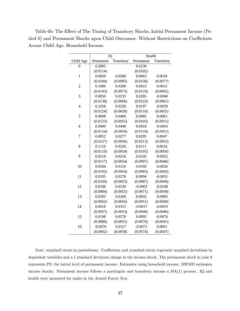
Table 6b: The E¤ect of The Timing of Transitory Shocks, Initial Permanent Income (Pe-

riod 0) and Permanent Shocks upon Child Outcomes: Without Restrictions on Coe¢ cients

Across Child Age. Household Income.

IQ HealthChild Age Permanent Transitory Permanent Transitory

0 0.2895 0.0230(0.0114) (0.0102)

1 0.0859 0.0280 0.0063 0.0034(0.0184) (0.0085) (0.0158) (0.0077)

2 0.1080 0.0288 0.0023 0.0053(0.0143) (0.0073) (0.0129) (0.0065)

3 0.0850 0.0235 0.0285 ­0.0040(0.0138) (0.0066) (0.0123) (0.0061)

4 0.1056 0.0258 0.0197 ­0.0029(0.0124) (0.0058) (0.0110) (0.0055)

5 0.0808 0.0406 0.0085 0.0003(0.0123) (0.0055) (0.0103) (0.0051)

6 0.0900 0.0448 0.0018 ­0.0003(0.0124) (0.0056) (0.0116) (0.0051)

7 0.0852 0.0277 0.0205 0.0047(0.0127) (0.0056) (0.0113) (0.0052)

8 0.1110 0.0226 0.0111 0.0014(0.0119) (0.0054) (0.0105) (0.0050)

9 0.0519 0.0216 0.0105 ­0.0052(0.0117) (0.0054) (0.0097) (0.0046)

10 0.0504 0.0150 0.0160 ­0.0026(0.0102) (0.0054) (0.0085) (0.0045)

11 0.0335 0.0276 0.0094 ­0.0031(0.0104) (0.0053) (0.0087) (0.0046)

12 0.0298 0.0330 ­0.0002 ­0.0108(0.0084) (0.0055) (0.0071) (0.0049)

13 0.0293 0.0269 0.0032 ­0.0085(0.0062) (0.0056) (0.0051) (0.0049)

14 0.0018 0.0313 ­0.0017 ­0.0010(0.0057) (0.0053) (0.0048) (0.0046)

15 0.0198 0.0270 0.0095 ­0.0076(0.0086) (0.0051) (0.0070) (0.0041)

16 ­0.0076 0.0317 ­0.0071 0.0001(0.0092) (0.0058) (0.0074) (0.0047)

Note: standard errors in parentheses. Coe¢ cients and standard errors represent standard deviations in

dependent variables and a 1 standard deviation change in the income shock. The permanent shock in year 0

represents P0, the initial level of permanent income. Estimates using household income. DWMD estimates

income shocks. Permanent income follows a martingale and transitory income a MA(1) process. IQ and

health were measured for males in the Armed Forces Test.

37

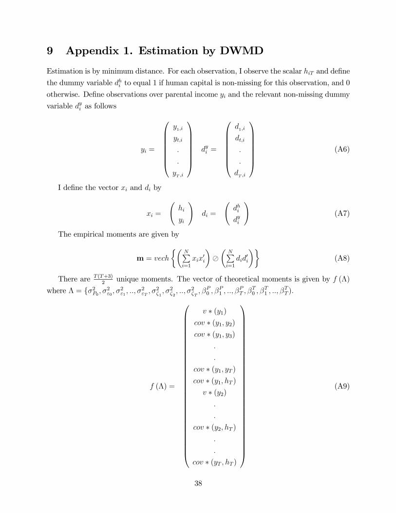
9 Appendix 1. Estimation by DWMD

Estimation is by minimum distance. For each observation, I observe the scalar hiT and de�ne

the dummy variable dhi to equal 1 if human capital is non-missing for this observation, and 0

otherwise. De�ne observations over parental income yi and the relevant non-missing dummy

variable dyi as follows

yi =

0BBBBBB@y1;i

yt;i

:

:

yT ;i

1CCCCCCA dyi =

0BBBBBB@d1;i

dt;i

:

:

dT ;i

1CCCCCCA (A6)

I de�ne the vector xi and di by

xi =

hi

yi

!di =

dhi

dyi

!(A7)

The empirical moments are given by

m = vech

��NPi=1

xix0i

���NPi=1

did0i

��(A8)

There are T (T+3)2

unique moments. The vector of theoretical moments is given by f (�)

where � = f�2P0 ; �2"0; �2"1 ; ::; �

2"T; �2�1 ; �

2�2; ::; �2�T ; �

P0 ; �

P1 ; ::; �

PT ; �

T0 ; �

T1 ; ::; �

TT ):

f (�) =

0BBBBBBBBBBBBBBBBBBBBBBBBBBBBB@

v � (y1)cov � (y1; y2)cov � (y1; y3)

:

:

cov � (y1; yT )cov � (y1; hT )v � (y2):

:

cov � (y2; hT ):

:

cov � (yT ; hT )

1CCCCCCCCCCCCCCCCCCCCCCCCCCCCCA

(A9)

38

Choose parameter values to minimise the di¤erence between the theoretical moments,

given in the identi�cation section above, and the empirical moments contained in m.

min�(m� f (�))0 �A (m� f (�))

The weighting matrix (A) is the diagonal from (V �1) ; where V is the variance-covariance

matrix of m, consequently estimation is diagonally-weighted minimum distance (DWMD).

References

[1] Adda, Jerome, James Banks, and Hans Martin von Gaudecker. 2009. "The impact of

income shocks on health: evidence from cohort data." Journal of the European Economic

Association, 7(6): 1361-1399.

[2] Akee, Randall K. Q., William E. Copeland, Gordon Keeler, Adrian Angold, and Jane

Costello. 2010. "Parents� incomes and children�s outcomes: a quasi-experiment using

transfer payments from casino pro�ts." American Economic Journal: Applied Eco-

nomics, 2(1): 86-115.

[3] Attanasio, Orazio, Erich Battistin, Emla Fitzsimons, Alice Mesnard, and Marcos Vera-

Hernandez. 2005. "How e¤ective are conditional cash transfers? Evidence from Colom-

bia." IFS brie�ng note 54.

[4] Attanasio, Orazio, Gabriella Berlo¤a, Richard Blundell, and Ian Preson. 2002. "From

earnings inequality to consumption inequality." Economic Journal, 112(478): c52-c59.

[5] Becker, Sascha. O, Samuel Bentolila, Ana Fernandes, and Andrea Ichino. 2010. "Youth

emancipation and perceived job insecurity of parents and children." Journal of Popula-

tion Economics, 23(3): 1047-1071.

[6] Black, Sandra, Paul Devereux, and Kjell Salvanes. 2008. �Too young to leave the nest?

The e¤ects of school starting age." IZA Discussion Paper 3452.

[7] Blundell, Richard, Luigi Pistaferri, and Ian Preston. 2008. "Consumption inequality

and partial insurance." American Economic Review, 98(5): 1887-1921.

[8] Blundell, Richard, and Ian Preston. 1998. "Consumption inequality and income uncer-

tainty." Quarterly Journal of Economics, 113(2): 603-640.

[9] Bonhomme, Stéphane, and Jean-Marc Robin. 2009. "Assessing the equalizing force of

mobility using short panels: France, 1990-2000." Review of Economic Studies 76(1):

63�92

39

[10] Cameron, Stephen V., and James J. Heckman. 2001. "The dynamics of educational

attainment for Black, Hispanic, andWhite males." Journal of Political Economy, 109(3):

455-499.

[11] Cameron, Stephen V., and Christopher Taber. 2004. "Estimation of educational bor-

rowing constraints using returns to schooling." Journal of Political Economy, 112(1):

132-181.

[12] Carneiro, Pedro, Kjell Salvanes, and Katrine Løken. 2010b. "A �ying start? Long-

term outcomes of maternal time investments in children during the �rst year of life."

Unpublished.

[13] Carneiro, Pedro, Kjell Salvanes, and Emma Tominey. 2010. "Better late than never?

The timing of income across children lives: A nonparametric approach." Unpublished.

[14] Chen, Stacey H., Yen-Chien Chen, and Jin-Tan Liu. 2009. "The impact of unexpected

maternal death on education: �rst evidence from three national administrative data

links." American Economic Review: Papers and Proceedings, 99(2): 149-153.

[15] Cunha, Flavio. 2005. "The complementarity and self-productivity of investments in

human capital in a stochastic dynamic general equilibrium economy with altruism and

lifetime liquidity constraints." PhD diss. The University of Chicago.

[16] Cunha, Flavio, and James J. Heckman. 2007. "The technology of skill formation."Amer-

ican Economic Review: Papers and Proceedings, 97(2): 31-47.

[17] Cunha, Flavio, and James J. Heckman. 2008. "Formulating, identifying and estimat-

ing the technology of cognitive and noncognitive skill formation." Journal of Human

Resources, 43(4): 738-782.

[18] Cunha, Flavio, James J. Heckman, and Susanne Schennach. 2010. �Estimating the tech-

nology of cognitive and noncognitive skill formation." Econometrica, 78(3): 883-931.

[19] Deaton, Angus. 1992. Understanding consumption. Baltimore: John Hopkins University

Press.

[20] Dickens, Richard. 2000. "The evolution of individual male earnings in Great Britain:

1975-95." Economic Journal, 110(460): 27-49.

[21] Farrell, Christopher, and William O�Connor. 2003. "Low-income families and household

spending." Department for Work and Pensions Research Report 192.

40

[22] Friedman, Milton. 1957. A theory of the consumption function. Princeton: Princeton

University Press.

[23] Ginja, Rita. 2009. "Income shocks and investment in human capital." Unpublished.

[24] Gregg, Paul, Jane Waldfogel, and Elizabeth Washbrook. 2006. "Family expenditures

post-welfare reform in the UK: are low income families starting to catch up?" Labour

Economics, 13(6): 721-746.

[25] Havnes, Tarjei, and Magne Mogstad. 2009. "No child left behind. Universal child care

on children�s long-run outcomes." Statistics Norway Discussion Paper 582.

[26] Hayashi, Fumio, Joseph Altonji, and Laurence J. Kotliko¤. 1996. "Risk-sharing between

and within families." Econometrica, 64(2): 261-294.

[27] Heckman, James J., Seong Hyeok Moon, Rodrigo Pinto, Peter A. Savelyev, and Adam

Yavitz. 2009. "The rate of return to the High/Scope Perry Preschool program." IZA

Discussion Paper 4533.

[28] Jappelli, Tullio, and Luigi Pistaferri. Forthcoming. "Financial integration and consump-

tion smoothing." Economic Journal.

[29] Jenkins, Stephen P., and Christian Schluter. 2002. "The e¤ect of family income during

childhood on later-life attainment: evidence from Germany." IZA Discussion Paper 604.

[30] Kaplan, Greg. 2007. "Moving back home: insurance against labor market risk." Unpub-

lished.

[31] Keane, Michael P., and Kenneth I. Wolpin. 2001. "The e¤ect of parental transfers and

borrowing constraints on educational attainment." International Economic Review, 42

(4): 1051-1103.

[32] Levy, Dan Maurice, and Greg Duncan. 2000. "Using sibling samples to assess the e¤ect

of childhood family income on completed schooling." JCPR Working Paper 168.

[33] MaCurdy, Thomas. 1981. "Asymptotic properties of quasi-maximum likelihood estima-

tors and test statistics." NBER Technical Paper 14.

[34] MaCurdy, Thomas. 1982. "The use of time series processes to model the error structure

of earnings in a longitudinal data analysis." Journal of Econometrics, 18(1): 83-114.

41

[35] Martins, Nuno, and Ernesto Villanueva. 2009. "Does high cost of mortgage debt ex-

plain why young adults live with their parents?" Journal of the European Economic

Association, 7(5): 974-1010.

[36] Meghir, Costas, and Luigi Pistaferri. 2004. "Income variance dynamics and heterogene-

ity." Econometrica, 72(01): 1-32.

[37] Møen, Jarle, Kjell Salvanes, and Erik Ø. Sørensen. 2004. "Documentation of the linked

employer - employee data base at the Norwegian School of Economics." Unpublished.

[38] Mo¢ tt, Robert, and Peter Gottschalk. 1995. "Trends in the covariance structure of earn-

ings in the US: 1969�1987.�University of Wisconsin Institute for Research on Poverty

Discussion Paper 1001�93.

[39] Parker, Jonathon A. 1999. "The reaction of household consumption to predictable

changes in social security taxes." American Economic Review, 89(4): 959-973.

[40] Paxson, Christina H. 1992. "Using weather variability to estimate the response of savings

to transitory income in Thailand." American Economic Review, 82(1): 15-33.

[41] Romich, Jennifer L., and Thomas Weisner. 2000. "How families view and use the EITC:

advance payment versus lump sum delivery." National Tax Journal, 53(4): 1245-1266.

[42] Rosenzweig, Mark R., and Kenneth I. Wolpin. 1993. "Intergenerational support and the

life-cycle income of young men and their parents: human capital investments, cores-

idence and intergenerational �nancial transfers." Journal of Labor Economics, 11(1),

Part 1: Essays in Honor of Jacob Mincer: 84-112.

[43] Shapiro, Matthew D., and Joel Slemrod. 1995. "Consumer response to the timing of

income: evidence from a change in tax withholding." American Economic Review, 85(1):

274-283.

[44] Souleles, Nicholas S. 1999. "The response of household consumption to income tax

refunds." American Economic Review, 89(4): 947-958.

[45] Sundet, Jon M., Dag G. Barlaug, and Tore M. Torjussen. 2004. "The end of the Flynn

e¤ect? A study of secular trends in mean intelligence test scores of Norwegian conscripts

during half a century." Intelligence, 32(4): 349-362.

42

[46] Sundet, Jon M., Kristian Tambs, Jennifer R. Harris, Per Magnus, and Tore M. Tor-

jussen. 2005. "Resolving the genetic and environmental sources of the correlation be-

tween height and intelligence: a study of nearly 2600 Norwegian male twin pairs." Twin

Research and Human Genetics, 8(4): 1-5.

43