Embed Size (px)
Citation preview

1
CELL BIOLOGY SIMULATION USING DEVS
COMBINED WITH SBML
By
Zhijie Wang
________________________
A Thesis Submitted to the Faculty of the
DEPARTMENT OF ELECTRICAL AND COMPUTER ENGINEERING
In Partial Fulfillment of the Requirements For the Degree of
MASTER OF SCIENCE
In the Graduate College
THE UNIVERSITY OF ARIZONA
2009

2
STATEMENT BY AUTHOR
This thesis has been submitted in partial fulfillment of requirements for an advanced degree at the University of Arizona and is deposited in the University Library to be made available to borrowers under rules of the Library.
Brief quotations from this thesis are allowable without special permission, provided that accurate acknowledgment of source is made. Requests for permission for extended quotation from or reproduction of this manuscript in whole or in part may be granted by the copyright holder.
SIGNED: Zhijie Wang
APPROVAL BY THESIS DIRECTOR
This thesis has been approved on the date shown below: Dr. Bernard P. Zeigler Date
Professor of Electrical and Computer Engineering

3
ACKNOWLEDGEMENTS
I would like to express my greatest appreciation to my advisor Dr. Bernard P.
Zeigler and Dr. Doohwan Kim, who introduced me to the fantastic world of discrete event simulation. Their support and encouragement on my research brought me so much insight which guides me to find my way in the world of computer simulation.
I would like to thank Dr. Roman Lysecky and Dr. Janet Wang for serving as my defense committee.
I would like to thank all the members at ACIMS, especially Dr. Saurabh Mittal
and Dr. James Nutaro for the useful discussion on my research. I would like to show special thanks to Ms. Jacky Wang, who helps and supports
me during my graduate study. I would like to express my wholehearted appreciation to my father and mother,
who never stop supporting and encouraging me. Special thank goes to my wife, Qingfen Zhang, for her constant support and
appreciation. I am indebted to her for all the encouragement. Finally, my daughter, Mindy Wang, make me never give up anything in my life.

4
Dedicated to my father and my mother
Jinzhan Wang and Junying Liu
for their selfless love and affection

5
TABLE OF CONTENTS
LIST OF FIGURES ............................................................................................................9
LIST OF TABLES ............................................................................................................12
ABSTRACT.......................................................................................................................13
CHAPTER 1 INTRODUCTION ......................................................................................15
1.1 Introduction ......................................................................................................... 15
1.2 Contributions........................................................................................................ 16
1.3 Organization...........................................................................................................17
CHAPTER 2 CELL BIOLOGY BACKGROUND AND SIGNIFICANCE ................... 19
2.1 Simulation of cellular processes........................................................................... 19
2.1.1 Metabolism.................................................................................................. 20
2.1.2 Signal transduction....................................................................................... 21
2.1.3 Gene expression........................................................................................... 22
2.1.4 Biophysical phenomena............................................................................... 23
2.1.5 Summary...................................................................................................... 23
2.2 Computational cell biology................................................................................... 24
2.2.1 Differences from conventional computational sciences.............................. 24
2.2.2 Computational cell biology research cycle.................................................. 25
2.3 Simulation methods in computational cell biology.............................................. 27
2.3.1 Ordinary differential equation solvers......................................................... 27
2.3.2 Special types of differential system solvers................................................. 41

6
TABLE OF CONTENTS-Continued
2.3.3 Stochastic algorithms for chemical systems................................................ 42
2.3.3.1 Chemical master equation................................................................... 43
2.3.3.2 Exact stochastic simulation algorithms............................................... 45
2.3.4 Other methods.............................................................................................. 50
2.3.5 Multi-algorithm simulation.......................................................................... 52
2.4 Existing software platforms and projects.............................................................. 55
2.4.1 General purpose simulation software........................................................... 55
2.4.2 Specialized simulation software.................................................................. 57
2.4.3 Software platforms and languages............................................................... 57
2.5 Systems Biology Markup Language..................................................................... 58
2.5.1 Structure of Model Definitions in SBML.................................................... 60
2.5.2 CellDesigner: a structured diagram editor................................................... 62
2.5.3 LibSBML..................................................................................................... 63
CHAPTER 3 DEVS AND DEVSJAVA.......................................................................... 65
3.1 DEVS.................................................................................................................... 65
3.1.1 DEVS and DEVS Formalism....................................................................... 65
3.1.2 Basic systems modeling formalisms............................................................ 73
3.1.3 Multi-algorithm framework......................................................................... 74
3.2 Differential Equation Models............................................................................... 77

7
TABLE OF CONTENTS-Continued
3.2.1 Basic Model: The Integrator........................................................................ 78
3.2.2 Continuous system simulation..................................................................... 80
3.3 Differential Equation Models in DEVSJAVA...................................................... 83
3.3.1 DEVSJAVA................................................................................................. 83
3.3.2 DEVS representation of discrete event integrators...................................... 84
3.3.3 Mapping Differential Equation Models into DEVS Integrator Models....... 88
3.3.4 DEVS Representation of Quantized Integrator in DEVSJAVA.................. 89
CHAPTER 4 DEVS COMBINED WITH SBML SYSTEM IN Cell BIOLOGY............91
4.1 Introduction........................................................................................................... 91
4.2 Layered Architecture of Cell Biology with DEVS and SBML............................ 92
4.3 DEVS with SBML Platform................................................................................. 95
4.3.1 DEVS-SBML Platform................................................................................ 95
4.3.2 The design of DEVS-SBML Platform......................................................... 96
4.3.3 The translator from SBML model to DEVS Model..................................... 97
4.3.4 DEVS-SBML GUI framework.....................................................................98
4.3.5 Modular Simulation Framework................................................................ 100
CHAPTER 5 RESULTS AND DISCUSSIONS.............................................................101
5.1 Introduction.........................................................................................................101
5.2 The efficiency analysis of DEVS-SBML Platform............................................ 102
5.2.1 Heat-shock model.......................................................................................102

8
TABLE OF CONTENTS-Continued
5.2.2 Efficiency analysis of the DEVS-SBML platform.................................... 105
5.2.3 ODE Deterministic Algorithm and Gillespie Stochastic Algorithm……..107
5.2.4 Performance analysis in the deterministic and stochastic schemes........... 109
5.3 The simulation procedure of DEVS-SBML Platform........................................ 111
5.3.1 Hypothetical single-gene oscillatory circuit in a eukaryotic cell............... 111
5.3.2 The simulation procedure of DEVS-SBML Platform................................113
5.3.3 Accuracy of DEVS-SBML simulation...................................................... 115
5.3.4 Error analysis in DEVS algorithm............................................................. 118
5.4 Discussions of DEVS algorithm......................................................................... 120
CHAPTER 6 CONCLUSIONS AND FUTURE WORKS............................................. 122
6.1 Conclusions......................................................................................................... 122
6.2 Future works....................................................................................................... 123
REFERENCES............................................................................................................... 126
APPENDIX A: SingleGene.xml......................................................................................137
APPENDIX B: Package singleGene using DEVS model ...............................................143

9
LIST OF FIGURES
Figure 2.1 Research cycle of computational cell biology................................................. 26
Figure 2.2 an SBML Document Structured...................................................................... 60
Figure 2.3 a model according to SBML............................................................................ 60
Figure 2.4 Reactions According to SBML....................................................................... 62
Figure 2.5 the skeleton of a model definition expressed in SBML.................................. 62
Figure 2.6 the user interface of CellDesigner ver.3.5.2.................................................... 63
Figure 3.1 Basic Entities and Relations............................................................................ 67
Figure 3.2 Discrete Event Time Segments....................................................................... 68
Figure 3.3 an Illustration for Classic DEVS Formalism................................................... 70
Figure 3.4 Basic Systems Specification Formalisms........................................................ 74
Figure 3.5 Multi-formalism Approaches.......................................................................... 75
Figure 3.6 DEVS and DESS combined model................................................................. 76
Figure 3.7 state event........................................................................................................ 77
Figure 3.8 Basic Integrator Concepts................................................................................ 78
Figure 3.9 the Integrator................................................................................................... 79
Figure 3.10 Structure of differential equation specified systems..................................... 79
Figure 3.11 Continuous system simulation problems....................................................... 80
Figure 3.12 Computing state values at time ti based on estimated values at time instants
prior and past time ti..................................................................................... 81
Figure 3.13 Mapping Differential Equation Models into DEVS Integrator Models........ 88

10
LIST OF FIGURES-Continued
Figure 3.14 DEVS simulator of a Quantized Integrator................................................... 90
Figure 4.1 Layered Architecture of System Cell Biology processes with DEVS and
SBML.............................................................................................................. 93
Figure 4.2 the Architecture of System Cell Biology processes with DEVS and SBML
......................................................................................................................... 94
Figure 4.3 Overview DEVS with SBML Platform Development…………………….... 96
Figure 4.4 Translator Modular from SBML model to DEVS model…………………….97
Figure 4.5 the GUI of the DEVS-SBML Simulation platform..........................................99
Figure 5.1 the heat-shock demonstration model............................................................. 103
Figure 5.2 Simulation results of the heat-shock model using DEVS ODE solver and the
E-cell system................................................................................................. 105
Figure 5.3 Simulation results of the heat-shock model using the DEVS ODE solver and
Gillespie stochastic algorithm....................................................................... 108
Figure 5.4 Schematic diagram of the single-gene oscillatory circuit model................... 112
Figure 5.5 the process diagram of the single-gene oscillatory circuit model using software
CellDesigner v3.5.2...................................................................................... 113
Figure 5.6 the DEVS viewer for the single-gene oscillatory circuit model.................... 114
Figure 5.7 Simulation results with Quantum Size (D) = 0.001 of all species for the single-
gene oscillatory circuit model....................................................................... 115
11
LIST OF FIGURES-Continued
Figure 5.8 Simulation results of the single-gene oscillatory circuit model for the DEVS
model and the CVODE model...................................................................... 118
Figure 5.9 DEVS simulation results analysis of AA for the single-gene oscillatory circuit
model............................................................................................................. 119
Figure 5.10 Execution time as a function of D for the single-gene oscillatory circuit
model................................................................................................................... 120

12
LIST OF TABLES
Table 2.1 some cellular processes and typical computational approaches ...................... 24
Table 2.2 Rough comparison of typical numbers characterizing various simulation targets
........................................................................................................................... 25
Table 2.3 Table 2.3 Butcher array for Runge-Kutta Fehlberg 2(3)...................................36
Table 3.1 Summary of Integration Method Speed-Accuracy Tradeoffs........................... 83
Table 5.1 Reactions list of heat-shock model................................................................. 103
Table 5.2 List of initial values used in heat-shock model .............................................. 104
Table 5.3 the results from the different tools in the heat-shock response....................... 106
Table 5.4 the results in the deterministic and stochastic schemes.................................. 110
Table 5.5 Reactions in the single-gene oscillatory circuit model................................... 112
Table 5.6 the initial value of Species list in the single-gene oscillatory circuit model....112
Table 5.7 the parameters of the reactions in the single-gene oscillatory circuit model...113

13
ABSTRACT
Computational cell biology is a relatively new branch of computational sciences
which sets computer simulation, as well as molecular biology, biochemistry and
biophysics, at the center of its disciplines.
This thesis first inspects this new field of science, cell biology, especially on its
computational aspects, and identifies some computational techniques in the design of
simulation algorithms and software platforms. One important characteristic of the
computational cell biology is that it is highly heterogeneous in terms of the modeling
formalisms and computational methods. Different simulation techniques are used for
different types of sub-systems in the cell, and these sub-systems are often represented by
different timescales. We found that the scientific necessity to integrate these
computational subcomponents to form the multi-formalism and composite models is
becoming increasingly important.
Secondly, this thesis proposes a novel computational framework based on discrete
event and differential equation combined with System Biology Markup Language
(SBML) to simulate the cell biological processes, which realizes efficient multi-algorithm
simulations. It is demonstrated that this framework can give a significant speed-up to a
real biological simulation model of E. coli heat-shock response by Discrete Event System
Specifications (DEVS) Ordinary Differential Equations (ODEs) solver combined with
SBML. It is also shown that this framework can boost the simulation of the single-gene

14
oscillatory circuit model. Some results of the numerical analysis and discussions for the
heat-shock and single-gene oscillatory circuit model are presented.
Lastly, this thesis describes the layered architecture, design and implementation
issues of DEVS-SBML Platform, a newly developed software environment for modeling,
simulation and analysis in computational cell biology, in which this computational
framework will be implemented as a future work.

15
CHAPTER 1 INTRODUCTION
1.1 Introduction
The advent of molecular biology in the twentieth century has led to exponential
growth in our knowledge about the inner workings of life. Dozens of completed genomes
are now at hand, and equipped with an array of high throughput methods to characterize
the way in which encoded genes and their products operate, we find ourselves asking
exactly how to assemble the various pieces. The question is whether we can predict the
behavior of a living cell given sufficient information about its molecular components. As
with any network of interacting elements, the overall behavior becomes non-intuitive as
soon as their number exceeds three. Computers have proven to be an invaluable tool in
the analysis of these systems, and many biologists are turning to the keyboard. It is worth
noting that the motivation of the biologist here is somewhat different from that of the
biologist who turns to computing for bioinformatics (such as sequence analysis).
Bioinformatics delivers additional information about the biopolymers being studied, and
may provide clues as to their function. What is sought in the analysis of cellular systems
is a reconstruction of experimental phenomena from the known properties of the
individual molecules, and more importantly, the interactions between them. Such a model,
if sufficiently detailed and accurate, serves as a reference, a guide for interpreting
experimental results, and a powerful means of suggesting new hypotheses.

16
Modeling, simulation, and analysis are therefore perfectly positioned for
integration into the experimental cycle of cell biology. In addition to demystifying non-
intuitive phenomena, simulation allows experimentally unfeasible scenarios to be tested,
and has the potential to seriously reduce experimental costs. Although “real” experiments
will always be necessary to advance our understanding of biological processes,
conducting “in silico” experiments using computer models can help to guide the wet lab
process, effectively narrowing the experimental search space.
The process of building in silico models of cells contrasts with the traditional
hypothesis-driven research process in biology. Modeling can be described as a holistic
approach that opposes the reductionism so widespread in biology. Molecular and cellular
biologists have been overwhelmingly successful in identifying, purifying, and
characterizing molecules crucial to specific cellular functions. However, results from
genome projects reveal that most organisms contain a surprisingly small number of genes,
at least relative to the complexity of the phenotype. This provides a striking
demonstration of the nontrivial nature of molecular interactions in the cell - the whole,
quite simply, is much more than the mere sum of its parts.
1.2 Contributions
The main contribution of this thesis is the introduction of a new technique,
Discrete Event System Specification (DEVS) framework combined with Systems
Biology Markup Language (SBML), to simulate biological processes. On this framework,
virtually any, discrete/continuous, stochastic/deterministic, simulation algorithms can be

17
implemented in biological simulations. More efficient method in biological simulation,
DEVS framework, is found.
Secondly, biological models can be shared between DEVS and SBML by DEVS-
SBML Platform, a Simulation Platform for computational cell biology. This simulation
software is under development in a fully object-oriented fashion based on the DEVS
algorithm framework combined with SBML.
As the rationale of development of these new computational frameworks and
software, this thesis also argues that computational cell biology has some major features
those distinguish itself from conventional computational sciences such as computational
physics and biochemical simulations.
1.3 Organization
Chapter 2 discusses a domain analysis of computational cell biology from the
viewpoint of simulation algorithm design and software engineering, and we identify
some ’desirable features’ of cellular simulation software. In Chapter 3, we reviewed the
basic DEVS concept and DEVS formalism. Multi-algorithm framework, the combination
of the DEVS and the Differential Equation System Specifications (DESS) formalism, was
introduced in this Chapter. The implementation of the integrator and Instantaneous
Functions to solve Differential Equations is given in DEVSJAVA Continuous package.
Chapter 4 defines a new computational framework to simulate biological processes,
called DEVS-SBML Platform. The architecture, design and some features of DEVS-
SBML Platform is shown. In chapter 5, we use two demonstration models, an E. coli

18
heat-shock model and a single-gene oscillatory circuit model, and find that the DEVS
algorithm can successfully combine SBML yielding considerable performance
improvements to the biological field. This chapter also has some discussions on DEVS
framework combined with SBML. The DEVS-SBML Platform will continue to be
implemented as a future work, a generic software suite for modeling, simulation and
analysis of cellular systems. Chapter 6 will give some conclusions for this thesis and
future works.

19
CHAPTER 2 CELL BIOLOGY BACKGROUND AND
SIGNIFICANCE
This chapter investigates the cell as a target of simulation, and discusses
computational challenges that it poses. Some simulation methods in the computational
cell biology were reviewed. We identify required features of cell biology simulators.
Multi-algorithm simulation was introduced in the computational cell biology. Existing
software platforms and projects also were reviewed. The definition of SBML was shown.
2.1 Simulation of cellular processes
The cell is a big system in terms of the number and the diversity of physical
phenomena that constitutes its internal dynamics. The small number of genes in most
organisms implies that molecular phenomena in the cell are, to say the least, nontrivial.
Collective knowledge of parts of the system itself does not directly lead to understanding
of the cell as a whole. Necessity and importance of cell simulation as a research method
arises here; putting the data into databases is not enough, only a more constructive
approach with computer modeling and simulation can provide a way to understand the
cell as a system.
In this section, we review such chemical and physical phenomena and discuss
some possible computational approaches to simulate these systems.

20
2.1.1 Metabolism
Energy metabolism is the best characterized part of all cellular behavior, and is
particularly well understood in human red blood cells. Given that an erythrocyte is devoid
of nuclei and other related features, it serves as an ideal model system for studying
metabolism in isolation — this cell is, essentially, “a bag of metabolism”. Biochemists
have succeeded in collecting enough quantitative data to allow kinetic models of the
entire cell to be constructed, and there is a long history of computer simulations dating
back to the 1960s [1]. These metabolic models, and many others, typically comprise a set
of ordinary differential equations (ODE) that describe the rates of enzymatic reactions.
These can be solved by numerical integration, for which several well-established
algorithms exist.
Modern metabolic pathway models typically consist of primary state variables for
molecular species concentrations, one ODE for each enzyme reaction, and a stoichio-
metric matrix. The rate equations of most modern enzyme kinetics models are derived
using the King-Altman method [2], which is a generalized version of the classical
formulation of Michaelis and Menten, the Michaelis-Menten equations [3]. Additional
algebraic equations are commonly employed as constraints on the system. Thus, most
metabolism models are described as differential-algebraic equations (DAE). The origin of
numerical methods for solving ODEs can be traced back to Euler’s work in the eighteenth
century. Variations of the Runge-Kutta method are generally used for simulations.
Implicit variations of the methods, are often used for ’stiff’ systems which involve a wide

21
range of time constants. See the following section for discussions about stiffness of ODEs.
Although there have been certain major advances in the last few decades, the essence of
the numerical algorithms for solving initial value problems of ODE systems was
described by Gear in 1971 [4]. Press et al. also give an introduction to the topic in
Numerical Recipes in C [5]. The theoretical and practical bases of simulating metabolic
pathways are therefore quite well grounded. However, the design and implementation of
simulation software and model construction methods, which this thesis attempts to
highlight, are still under active discussion.
Metabolism, of course, is not the only function of the cell, and we must not forget
that cells have other important roles such as gene expression, signal transduction, motility,
vesicular transport, cell division and differentiation. Although quantitative data on these
processes are still relatively sparse compared to erythrocyte energy metabolism, certain
systems have been modeled with considerable success. Examples include the simulation
of gene expression in phage-λ [6] and the signal transduction pathway controlling
bacterial chemotaxis [7].
2.1.2 Signal transduction
Signal transduction pathways constitute an example of systems with
characteristics that prevent the simple application of ODE-based modeling. These
pathways are ordinarily composed of much fewer numbers of reactant molecules than
metabolic systems, and the underlying stochastic behavior of the molecular interactions
becomes evident. Accordingly, there have been attempts to model signal transduction

22
pathways with stochastic computation [8] [9] instead of deterministic methods (e.g. use
of ODEs).
Recently, it has been revealed that two-dimensional stochastic coupled lattice
model of receptor localization of E. coli chemotaxis signaling better explains the
system’s hyper sensitivity to stimuli that could not be reproduced by conventional
compartmental simulations [10].
2.1.3 Gene expression
Gene expression systems, like signaling pathways, tend to be composed of a small
number of molecular entities, which include transcription factors, polymerases, and genes.
These low copy number molecules orchestrate gene expression in a highly stochastic
fashion. For example, the initial phase of gene expression is remarkable because its
stochastic behavior has binary consequences: binding of a rare transcription factor and a
single gene in a cell can determine whether the gene is turned on or off. It seems that in
many cases, gene expression systems might best be modeled with stochastic equations,
although there are many other ways to model these phenomena, depending on the
modeler’s interests. Examples include ODE models (e.g. linear models and mass action
models), S-System models [11], and binary and multi-reaction models [12].
Another characteristic of gene expression systems is the richness of interaction
with other cellular processes. These systems can control metabolic flux by changing the
concentrations of enzymes, and at the same time being regulated by signaling proteins.
Chromosomal structure is dynamically regulated by DNA binding factors, which are in

23
turn derived from other genes. When a whole cell is modeled, elements in the gene
expression system sometimes need information about elements in other systems, in order
to allow cross-system interactions. Integration of gene expression and other systems at
the whole cell level might best be accommodated by object-oriented data structures, as
previously described in Hashimoto et al. [13].
2.1.4 Biophysical phenomena
All of the above simulation examples treat the properties of protein binding and
enzyme kinetics reactions. However, certain cellular processes such as cytoskeletal
movement and cytoplasmic streaming need to be modeled at the biophysical level.
Cytoplasmic streaming involves diffusion of relatively heavy proteins, whereas the
movement of the cytoskeleton causes structural changes, including cell division and cell
differentiation. Simulations of these phenomena have been carried out since the 1970s
[14]. Studies have become more precise with time, concomitant with the increase in our
depth of understanding at the molecular level [15].
2.1.5 Summary
A few types of cellular processes and typical computational approaches are shown
in Table 2.1. The interested reader is referred to two recent reviews which address some
of the issues raised thus far: Tyson et al. provide an excellent review of computational
cell biology with an emphasis on cell-cycle control [16], while Phair and Misteli review
the application of kinetic modeling methods to biophysical problems [17].

24
Table 2.1 some cellular processes and typical computational approaches Process type Dominant phenomena Typical computation schemes Metabolism Enzymatic reaction DAE, PL, FBA, CA
Signal transduction Molecular binding DAE, stochastic algorithms (StochSim, Gillespie), diffusion-reaction
Gene expression Molecular binding, polymerization, degradation
OOM, PL, DAE, Boolean networks, stochastic algorithms
DNA replication Molecular binding, polymerization
OOM, DAE
Cytoskeletal dynamics Polymerization, mechanical forces
DAE (including mechanical models), particle dynamics, OOM
Cytoplasmic streaming Streaming CA (e.g. lattice Boltzman), PDE Abbreviations: CA, Cellular Automata; DAE, differential-algebraic equations (rate equation-based systems); FBA, flux balance analysis; OOM, object-oriented modeling; PL, power-law, such as S-System and Generalized Mass Action.
2.2 Computational cell biology
2.2.1 Differences from conventional computational sciences
Software development for non-trivial cell simulation projects is a notably
expensive process. For research projects in the traditional computational sciences, where
brute force computation remains operative, it is reasonable to develop new software for
each project, sometimes in a disposable fashion. Most of the traditional computational
science fields like computational physics are characterized by numerous uniform
components and a limited number of simple principles. Cell simulation, in contrast,
involves numerous and various components with different properties, interacting in
diverse, complicated manners. Typical characteristics of several simulation targets are

25
summarized in Table 2.2. The design and implementation of simulation software
inevitably reflects the complexity of the problem.
Table 2.2 Rough comparison of typical numbers characterizing various simulation targets Target Compartments Components Component
types Interaction
modes Prokaryotes
(E. coli) ~101 ~1013−14 molecules
~103−4 species ~101(1) ~101−3(2)
Eukaryotes (H. sapiens)
~103−4 ~1017−18 molecules ~104−5 species
~101(1) ~101−4(2)
LSI (Electronic
circuit)
usually 1 ~106−7 a few 1
CFD (Fluid dynamics)
usually 100−1 ~105−6 1 1
MD (Molecular dynamics)
1 ~102−6 a few a few
Some typical numbers, which determine computational hardware and software requirements, are compared among several simulation targets. Large numbers of compartments, component types and interaction modes characterize cell simulation. Notes: (1) Component types which require different data structures or object classes are counted. For example, a ’membrane’ object needs a different object class from protein molecules. Different molecular species, however, are not counted. (2) This number depends on whether or not different enzyme kinetics equations, which are roughly proportional to the number of enzyme encoding genes, are counted as different interaction modes. Interaction modes other than enzymatic reactions include molecular bindings (complex formations), molecular collisions, DNA replication, cytoplasmic streaming, cytokinesis, and vesicular trafficking.
2.2.2 Computational cell biology research cycle
We envision a research cycle of cell biology that incorporates bio-simulation
technology (Figure 2.1). Every step of the cycle completed outside of the wet lab depends
upon sound methods in software engineering. Consider the storage, processing, and
utilization of massive amounts of biological knowledge: only through integration of an

26
intelligent modeling environment with sophisticated data and knowledge bases can the
challenge of modeling a very large and complex system be accommodated. Although this
thesis mainly considers the first half of the cycle (from ’Qualitative Modeling’ to ’Run’),
a technological stagnancy in any one of the steps may form a bottleneck, and thus
threaten the evolution of computational cell biology.
Figure 2.1 Research cycle of computational cell biology
The wet lab process is extended to include simulation software for a computational cell biology research project. Qualitative models (e.g. pathway maps) are built from in vivo and in vitro data and hypotheses, or a reference model (Qualitative Modeling). Then, quantitative characterization of cellular properties facilitates the transition to a mathematical system model (Quantitative Modeling). The numerical and discrete properties of the quantitative model are translated into a modeling language (Cell Programming), and the systemic behavior is predicted (Run). Results are then analyzed to suggest new hypotheses (Analysis and Interpretation). Any acquired hypothesis is subsequently tested by wet experiments, and the cycle begins a new.

27
2.3 Simulation methods in computational cell biology
As we have seen, simulation of the cell requires heterogeneous approaches
according to the levels of abstraction, scales, and types of information available to
construct simulation models. Here we briefly review some commonly used numerical
simulation techniques.
2.3.1 Ordinary differential equation solvers
Ordinary differential equations (ODEs) are one of the most popular ways of
describing continuous dynamical systems. A distinct strength of this formalism is that,
with its well-established theory in numerical treatments and availability of high-
performance generic solvers described in the following, it can represent virtually any
continuous and deterministic dynamics elegantly.
In computational cell biology, the most popular use of ODE formalism is the
macroscopic representation of chemically reacting systems by a means of kinetic rate
equations. Elementary and some simple reactions are represented in a form of mass-
actions, for example,
X1 + X2 X3, (2.1)
and it can be formulated by using the following differential equation
]][[][][][ 21321 XXkXdt
dX
dt
dX
dt
d , (2.2)
Where Xn is the n-th chemical species ([·] denotes concentration), and k is the rate
constant. Complex enzymatic reactions are often modeled by using Michaelis-Menten

28
and King-Altman types of rate equations. The Michaelis-Menten equation corresponding
to the following simplest enzymatic reaction mechanism
E + S ES → E + P, (2.3)
is
][
][
SK
SEKP
dt
dS
dt
d
m
Tcat
, ET = E + ES, (2.4)
Where S, P, and E are the substrate, product, and enzyme, respectively, and Kcat is the
catalytic constant (the turnover number of the enzyme), and Km is the Michaelis constant.
Unlike some of other specialized formalisms introduced in the following sections,
most differential equation solvers are generic, and can handle a variety of linear and
nonlinear equations employed in cell biology. Some examples of representations of those
phenomena other than rate equations include dynamic changes in environmental factors
such as thermodynamic parameters temperature, pH, and volume
Initial value problems of ODEs
A system of ODE has a general form like this:
00 )(),,( xtXxtfXdt
d (2.5)
Where x is a vector of dependent variables, f is a vector of derivative functions, and t is
an independent variable. In time-driven simulations, the independent variable t is usually
time. The system is autonomous if the system does not explicitly depend on the
independent variable t;

29
)(xfXdt
d (2.6)
Time simulation of ODE systems is equivalently reformulated as solving (2.5) for X(t),
where t R+, 0.
Taylor expansion of X in (2.5) at time t0 gives
000 ),(!
)()( ttttXdt
d
i
ttXtX
i
ii
i
(2.7)
or,
00)1(
)1(
0 ),(!
)()( ttttfdt
d
i
ttXtX
i
ii
i
(2.8)
If analytical differentiation of the system f to arbitrary high order can be derived, this
Taylor expansion immediately gives the solution, or the simulation trajectory, X(t).
Practically, however, ODE representations of biological problems often make use of
nonlinear equations, and it is very hard to construct a general method of solving these
equations analytically. Thus use of iterative numerical methods is the norm. This class of
the problem is called the initial value problem (IVP) of ODEs.
Numerical solution of ODEs has a considerable history, and the oldest and
simplest method was given by Euler in 1768 [63]. From the definition of derivatives,
,lim1
1
0nn
nn
t tt
XXX
dt
d
(2.9)
Where
,1 nn ttt (2.10)
Now for sufficiently small t we can assume that this formula gives an
approximation of the derivatives at the time point tn,

30
nn
nnnnnt tt
XXXtff
dt
dXn
1
1)),((| (2.11)
Comparing this with (2.5),
Xn+1 = Xn + ∆t · f (tn, Xn) (2.12)
We now get the explicit Euler method. It is called explicit because no unknown
appears in the right hand side (RHS) of the equation (2.12).
Consistency and Convergence
Two requisite properties of a numerical method to be useful are consistency and
convergence.
A numerical method is consistent when the local truncation error,
e ≡ |X<tn> (tn+1) – Xn+1|, (2.13)
diminishes to zero as the step size decreases:
,0lim0
et
(2.14)
where e is a vector of the local truncation errors of each variable of the system xi x.
Here x < tn > (tn+1) is the exact solution with the initial condition x(tn) at time tn. Proof of
consistency of the explicit Euler method is trivial. Using (2.10), (2.11), and assuming xn
= x (xtn), the local truncation error of the method is obtained from (2.12) as
|)(| 11eulernn
euler XtXe
|)()()(!
)(|)1(
)1(
nnni
ii
in tftXtf
dt
d
i
ttX
(2.15)
|)(!
|2:
)1(
)1(
iNii
ni
ii
tfdt
d
i
t (2.16)

31
It can be verified that eeuler 0 as t 0, hence the explicit Euler method is
consistent. Third and higher components are ignorable when t is sufficiently small, thus:
|)(2
1|2
neuler tf
dt
dte (2.17)
Consequently, it can be seen the error of the method has an order of t2. Thus, a more
formal formulation of the method comes with the local error term of O(t2):
X(tn+1) = Xn + ∆t · f(tn, Xn) + O(∆t2) (2.18)
In simulation, the global truncation error, which indicates accumulation of the local error
after certain period of time, is of practical importance. The global truncation error of a
method is given by
E ≡ |X(ti) - Xi| (2.19)
For simplicity, assuming the step size t is constant, the simulation requires (t)−1
iterations for a unit of time. Thus, the accumulation of the error can be denoted as
E = (∆t)-1 · e (2.20)
It can be read that generally the global truncation error is of order p with respect to the
step size t, when the local truncation error is O(tp+1). If a method has the global
truncation error of O(tp), then it is said to be consistent with an order of accuracy p. The
explicit Euler method therefore has a consistency of the first order.
One of the most important design goals of numerical methods is to get a good
convergence with as small as possible computation cost. A method is said to be
convergent if
0|)(|lim:0
ii
tXtXi (2.21)

32
Non-convergent methods are of no use because qualities of outcomes of simulations are
not assured.
Higher order methods
Computation cost of numerical methods is proportional to the inverse of the step
size, 1/t. One way of increasing the step size without a directly proportional increase in
the error is use of methods of higher order consistency. Many algorithms of the second,
higher, and variable consistency order have been proposed and being used, and most of
them can be classified into two categories: single- and multiple-step methods. Multi-step
methods make use of the information calculated in some past steps to conduct the current
simulation step. Single-step methods are ’closed’ in this sense; these methods utilizes
only the current state of the system. Although historically the multi-step methods once
had been a standard, and many popular software packages including LSODE and DASSL
are based on this class of methods, recent advancements in single-step methods,
especially variants of the Runge-Kutta method [63], is changing the picture. When the
applications in computational cell biology simulation is under consideration, single-step
methods have some favorable features over the multiple-step methods; it is (1) easier to
implement the real-time user interaction efficiently, and (2) better suited in uses in
conjunction with other algorithms in multi-formalism simulations (see the next section).
Also, it often results in simpler implementation, and unlike multi-step methods, no
special procedure is necessary in simulation start up. For those reasons, here mainly
discusses about the Runge-Kutta methods.

33
The general form of an s-stage, single-step Runge-Kutta method is:
s
jjjnn
s
iiijnjnj
kbtyy
sjkatytctfk
11
1, ...1),,(
(2.22)
Where a, b, and c are called Runge-Kutta coefficients, or collectively Butcher array.
Setting s = 2, a second-order explicit Runge-Kutta method can be derived in this way:
Xn+1 = Xn + ∆t · (b1k1 + b2k2), (2.23)
k1 = f(tn, Xn), k2 = f(tn + c2 ∆t, Xn + ∆t k1 a2,1) (2.24)
where a2,1, b1, b2, and c2 are the Runge-Kutta coefficients to be decided. Now Taylor
series expansion of k2 to the first order gives
nn ttn t
fatk
t
ftcfk || 1,2122
(2.25)
Putting (2.25) into (2.23),
)||()( 1,22222
211 nn tntnnn t
ffab
t
fcbttfbbXX
(2.26)
Now we want to compare this with the Taylor series (2.8), which, curtailing the third and
higher order terms, becomes:
fdt
dttfXX nn 2
22
1 2
(2.27)
)(2
2
x
ff
t
fttfX n
(2.28)
Then we now have three equations for the four coefficients;
b1 + b2 = 1, b2c2 = ½, b2a2,1 = ½ (2.29)

34
These relations are under determined, and there can be infinite number of second-order
explicit Runge-Kutta methods. For example, setting b1 = 0 gives the midpoint method
)2
),(,
2(1
nnnnnn
XtftX
ttftXX
(2.30)
In this way, higher order methods of arbitrary high order can be derived from
comparison between (2.22) and the Taylor series. Use of higher order methods is
preferable. As it can be understood from the equation (2.8) of the Taylor series, the scale
of error term decreases rapidly with regard to the order of the method, and we can take
exponentially large step sizes with the same level of truncation error. This in turn means
that we can complete the simulation with less number of steps, and therefore less
accumulation of round-off error.
It is known, however, the fourth order is a kind of optimum and most frequently
used. Up to the fourth order it just requires the same number of stages of right-hand side
evaluations as the consistency order, while fifth and higher order methods involve more
stages than the order of the method. For example, at minimum 6 stages are necessary for
the fifth order method, s = 7 for sixth order, s = 9 for seventh, and s = 11 for eighth.
Error control
A commonly used error control scheme of numerical methods is based on the
local truncation error as follows:
|)),|||((|:| iirelabsi ftbxasafetyei (2.31)

35
Where ei e is the error of this step of the variable xi, safety is a safety factor (usually ~
110%), σabs and σrel are absolute and relative error tolerances, a and b are scaling factors
for the value and derivative of the variable, respectively. In each step, numerical methods
control the error by means of the step size and other parameters such as the order of the
calculation. If the error of at least one variable violates the criteria (2.31), the solver
rejects the step and redoes the calculation with a shrunken step size. Conversely, if the
error is sufficiently smaller (say, ~ 50%) than the right hand side of (2.31), the step size
can be elongated to reduce the computation cost. There can be many strategies of
deciding step sizes. Two most frequently used methods are step halving/doubling and
variations of the following basic equation
,|| /1 s
n
nnew e
xTolerancett
(2.32)
where Tolerance is the right hand side of (2.31), and n is the index of the variable which
gave the maximum error in the current step. It must be noted that generally it is
impossible to obtain the exact values of the local truncation errors, and an integrator must
somehow numerically estimate the en.
A frequently used strategy to estimate the local error is to have a pair of Runge-
Kutta calculations of orders p and p + 1. The difference between solutions from these
calculations gives a good approximation of the local error, because as the Taylor series
expansion implies, the value of error term diminishes rapidly to the order. A neat trick to
obtain this estimation of the local truncation error efficiently is the embedded Runge-
Kutta method, devised by Fehlberg [18]. The underlying idea is to embed a Runge-Kutta

36
calculation of the order p into that of the order p + 1. Table 2.3 is the Butcher array of a
method called Fehlberg 2(3), which specifies Runge-Kutta coefficients. Calculating the
equation (2.22) using the coefficient in the bi and b*i columns give the second and the
third order solutions, respectively, and it requires only three RHS evaluations.
Table 2.3 Butcher array for Runge-Kutta Fehlberg 2(3)
Stability and stiffness
Some differential systems are stiff. Although stiffness is not defined in a
mathematically rigid way, here we give it a casual definition as follows: when the system
has at least two very different time scales, and the trajectory is dominated by the slow
movement, then it is stiff. To put this in a bit more formally, if the fast mode of the
system has a stable manifold, and the state point of the system is captured by it, the
system is stiff. Thus a system can become stiff and non-stiff according to where the state
point is. For example, when the system is making a transition from one state point to a
distant stable manifold, it is non-stiff, while as long as the trajectory is on the manifold, it
is said to be stiff.
Stiffness can be understood in terms of the Jacobian matrix which is

37
x
fJ
(2.33)
Stiffness is sometimes defined as
1||
Ctx
f (2.34)
where C is a positive constant which represent a typical number of simulation steps (say,
106 or 1012).
When the system is stiff, all the explicit methods explained so far experience
hardship. Consider the exact solution at time tn, x(tn), on the slow manifold. All the
explicit methods primarily uses values of the derivative functions at the current state
point of the numerical solution, xn, to estimate the state of the system after the some
amount of time t. Any numerical computation involves some amount of error ε, and it
puts the numerical solution slightly off the slow manifold, thus, xn = x(tn) + ε. When the
Jacobian is very large, this error ε magnifies the error in the next numerical solution point
xn+1, and the assumption behind (2.20), that is, the global error is a simple accumulation
of the local error, no longer holds. Although the convergence of the computation (2.21)
itself is not necessarily affected, the effectiveness of the error control scheme in (2.31) is
destroyed. Because slow manifolds are often stable, the fast flows toward the center of
that manifold appear in values of Jacobian around there, and in this case the trajectories
disastrously show diverging oscillations. Even if the solver managed to detect the error in
the step, it results in frequent step rejections, and forces the solver to take extremely
small step sizes to converge.

38
A measure of tolerance against stiffness is stability of numerical methods.
Consider a scalar system
)(xfdt
dx (2.35)
If the system is linear,
xdt
dx (2.36)
the stability of a method is defined by the stability function R(·), which is defined as
nn xtRx )(1 (2.37)
In the case of the explicit Euler method it is,
nn xtx )1(1 (2.38)
Setting t · λ = z,
nn xzx )1(1 (2.39)
Thus the stability function of the method is
R(z) = 1 + z (2.40)
Now the stability region of the method is given by
|R(z)| = |1 + z| ≤ 1 (2.41)
and it is shown that the explicit Euler method is stable only in a very narrow range −2 ≤
t · λ ≤ 0. More generally, when it is a linear vector system, the constant λ is an eigen
value of the constant coefficient matrix A in
XAdt
dX (2.42)
and thus a complex number.

39
Use of implicit methods overcomes this stability problem. The implicit Euler
method, in a scalar form, has the following form:
),( 11 nnn xtfxx (2.43)
Putting the linear scalar system (2.36) into this and rearranging to the form of the
stability function (2.37) gives the stability function of this method:
nn xz
x )1
1(1
(2.44)
Therefore this method is stable in the region |1 − z| ≤ 1, or, it is stable in an open region
except for the domain 0 < t · λ < 2 in the case of the scalar system.
If the stability region of a method includes the whole left-half of the complex
plane of z, which is the case of the implicit Euler method, it is called absolutely stable, or
A-stable. That is, when the real part of λ is zero or negative, the method is guaranteed to
be stable. Similarly, if the same condition is satisfied for general non-linear systems, it is
said to be B-stable. The order of the global error of the method for the general non-linear
systems is called B-convergence.
The exact solution of the linear problem (2.36) at the next time point tn+1 is easily
derived as eλt xn. Now recall the definition of the local error (2.13) again, and using
(2.37):
|))((|1 nz
n xzRee (2.45)
A method is called stiffly accurate if
0|))((|lim||
n
z
zxzRe (2.46)
Now check if the implicit Euler method is stiffly accurate:

40
0|1
1|lim
||
zez
z (2.47)
If a method is both A-stable and stiffly accurate, it is said to be L-stable or stiffly
A-stable or strongly A-stable. The point here is that no matter how large the damping
force of the system is (even in the case it is infinite), the numerical solution does not, at
least, diverge. This property is important in very stiff problems and some DAE systems.
It is desirable that all numerical methods used are L-stable, but only a few A-stable
methods are known to be L-stable.
Implicit methods
Implicit Euler method imposes solution of non-linear equations to conduct a step
of computation. Newton’s method [19] is most popularly used for this purpose. A
Newton iteration to get xn+1 of (2.43) using the first order Taylor series expansion is:
)(|),( 111),(
1111 1
11
mn
mnXt
mnnn
mn XX
X
ftXttfXX m
nn (2.48)
or in a programmable form,
1
),(
11),(
1111 )|(]|),([ 1
111
11
mnn
mnn Xt
mnXt
mnnn
mn X
ftIX
X
ftXttfXX (2.49)
where m is the counter of the Newton iteration, and I is an identity matrix. The iteration
is terminated when the difference |x m n+1 − xm−1 n+1| goes below a pre-defined threshold.
In the same way, it is possible to derive implicit variations of higher order methods.
Despite their good stability of implicit methods that is necessary to solve stiff
systems efficiently, a drawback is computation cost. In addition to that of its explicit

41
counterpart, it requires m iterations of (2.49) involving a calculation of the Jacobian
matrix and a matrix inversion. Generally, in non-linear computational cell biology
problems, Jacobian cannot be obtained analytically, and numerical differentiation is
necessary. Although the precision of this calculation of Jacobian does not affect the
accuracy of the simulation itself as long as the Newton iteration converges, the cost of
this computation is not negligible. The computation cost of a matrix inversion is in the
order of O(N 3), where N is the size of the matrix. N becomes proportionally bigger when
higher order methods such as implicit Runge-Kutta are used.
Therefore, a good ODE simulator is supposed to be able to adaptively switch
between explicit and implicit methods automatically detecting stiffness of the system.
The best combination that this thesis suggests is a pair of the fourth order Runge-Kutta
with adaptive step-sizing such as Dormand-Prince [20] or Runge-Kutta Fehlberg [18]
method and Radau IIA [21] methods. Radau IIA is the best implicit Runge-Kutta
equation ever known, and is L-stable, and B-convergent of the order s for the consistency
of 2s − 1. Three-stage (s = 3) version of Radau IIA with the fifth order consistency,
sometimes called Radau 5, is often used.
2.3.2 Special types of differential system solvers
In cellular and biochemical simulations, specialized differential equation solvers
are sometimes used. For example, power-law canonical differential equations are often
used to model various types of cellular phenomena such as gene expression and
metabolic systems. Two of these formalisms are S-System:

42
,,...,1,11
,, Nixxxdt
d n
j
hii
n
j
giii
jiji
(2.50)
where N is the size of the system, and αi, βi, gi,j, hi,j are S-system coefficients, and
Generalized Mass Action (GMA):
,,...,1,1
, Nixxdt
d n
j
fiii
ji
(2.51)
where i and fi,j are GMA coefficients.
A distinct feature of this kind of formalisms is that it does not distinguish the
structure of the system from its dynamics. The whole properties of a system can be
described by a single S-System or GMA matrix. When used in simulation, it provides
good means of estimating the network structure of the system as well as kinetic orders. In
other words, by using S-System and GMA formalisms, the difficult problem of network
structure determination can be converted to a matter of numerical parameter estimation,
which is compatible with well established technique of non-linear optimization with
numerous powerful algorithms such as Genetic Algorithms and the modified Powell
method. A special algorithm called ESSYNS method can be used to solve these power-
law systems efficiently [22].
2.3.3 Stochastic algorithms for chemical systems
All numerical treatments explained above are continuous and deterministic, which
means that those descriptions of chemical processes are macroscopic and approximate.
Chemical systems are, at the bottom, composed of discrete molecules, and the
assumption behind differential formalisms that state variables change continuously and

43
their trajectories are differentiable does not hold, and thus, the differential descriptions
fail to correctly reproduce the stochastic fluctuation in the number of molecules that
becomes evident when copy numbers of involving molecular species of reactions are
small.
Some variations of stochastic simulation algorithms for chemically reacting
systems in some exact consequences of the chemical master equation are introduced here.
Also stochastic simulation methods can be approximate using many possible ways. One
of the best known procedures is given in Gillespie and Petzold [23].
2.3.3.1 Chemical master equation
Consider a finite and fixed volume Ω in which M reaction channels connect N
molecular species. Temperature and other physical parameters that affect the reaction rate
are all constant. In meso-scopic representation of the system, we do not track motion of
each molecule. Then the state of the system is a vector of random variables X(t) NN. It
also assumes that occurrences of non-reactive collisions are so frequent that (1) it stirs the
system between any two reactive collisions, and (2) each occurrence of reaction is a
Markov process. Strictly speaking, in cell biology, most systems are in liquid phase and,
unlike gas phase, once two solute molecules encounter, it is highly probable that these
molecules experience numerous successive collisions because of the existence of solvent,
making reactions non-Markovian. However, here we neglect this in the following
discussions because experiences so far have shown that we can construct precise
simulation methods without taking this non-Markovian argument into account.

44
Now the propensity function
aj(X)dt (2.52)
is defined as the probability that the j-th reaction will occur in Ω in an infinitesimal time
interval [t, t + dt), given X = X(t). The state change vector
νj, (2.53)
whose each element νj,i specifies the number of molecules of the i-th species changed by
an occurrence of the j-th reaction.
If the reaction is elementary, the propensity function has the following form:
aj(X) = cj ηj, (2.54)
where cjdt gives the probability that a pair of reactant molecules will collide and react in
a unit time interval, and ηj is the number of distinct combinations of such reactant
molecules in the state X. If the reaction has the form of (1) X1 → X2 · · ·, ηj = X1, if it is (2)
X1 + X2 → X3 · · ·, then ηj = X1X2, and if (3) 2X1 → · · ·, then ηj = max(X1(X1−1)/2, 0). The
macroscopic rate constant kj of the reaction is related with cj in: (1) kj = cj, (2) kj/Ω = cj,
(3) 2kj/Ω = cj.
Given the propensity function and the state change vector, an exact and complete
description of the chemically reacting system evolving from the initial condition X0 at
time t0 can be derived:
M
kkkkk tXXPXatXXPXatXtXP
t)],|()(),|()([),|,( 000000 (2.55)

45
This is called the chemical master equation (CME). This formalism was initially
proposed as a simple stochastization of macroscopic rate equations [24], but has recently
given a rigid micro-physical ground [25].
By definition of X, (that is NN), CME (2.55) is a system of a huge number of
differential equations, and cannot be solved in any way (analytical or numerical) unless it
represents a very simple system (for example, a single ion channel whose state is either
open or close).
2.3.3.2 Exact stochastic simulation algorithms
Although the CME describes everything about a chemical system, it cannot be
used in simulations directly. What we need is a method of trajectory realization based on
the CME, which does not require evaluation of the whole state space defined in the
system. One way to reduce the computation cost to a point where we can handle with our
digital computers is a kind of lazy evaluation, which is, at each simulation step,
calculating the values of propensity functions at neighboring state points to the current
state point.
Gillespie proposed the next reaction density function [26] [25],
))(exp()(),|,( XaXatXjpM
kkj (2.56)
which defines the probability that the next reaction in the system occurs in the
infinitesimal time interval [t + τ, t + τ + dτ), and the reaction is the j-th reaction.

46
With this next reaction density function, a step of simulation is defined as a
procedure of generating a pair of numbers (τ, μ), that indicates the step size and the state
transition difference function X(t + τ) = X(t) + νj. There can be some possible ways of
generating this real-integer pair of random numbers, and one of the straightforward ways
is called the Direct method. The joint density function (2.56) can be rewritten as a
composition of two simple functions for τ and j, respectively.
),|(),|(),|,( 21 tXptXptXp (2.57)
where p1(τ |X, t) is the probability that the first firing of any of the reaction channels
occurs at time t + τ, and p1(μ | X, t) is the probability that μ is the reaction that fired.
These two functions are defined as:
,))(exp()(),|( M
k
M
kkk XaXatXP (2.58)
,)(/)(),|Pr( M
kk XaXatX (2.59)
In numerical computer simulations, a type of random numbers that is available in
the most efficient way is the uniform, unit-interval random distribution U(0, 1). To
generate τ according to (2.58) from a sample of the uniform distribution, u1, the following
Monte Carlo inversion function of (2.58) is used:
),1
ln())((1
1
uXa
M
kk (2.60)
Determining μ is then a simple task. Using another number u2 taken from the uniform
random number generator,

47
)X()X(:min 2 l
l
n
kk auaNnn (2.61)
Main portion of the computation cost of the Direct method comes from two random
number generations and calculation of M propensity functions per a simulation step.
Here is a procedural definition of the Gillespie’s Direct method:
1. Initialize: set initial number of molecules, and reset t (t ← 0).
2. Calculate the values of the propensities (ai) for all the reactions.
3. Choose τ according to (2.60).
4. Determine the next reaction μ according to (2.61).
5. Change the number of molecules: X ← X + νμ.
6. t ← t + τ.
7. Go to (2).
Another approach to the generation of the (τ, μ) pair is the First Reaction method,
also devised by Gillespie [26]. It generates tentative τ s for all reaction channels,
),1
ln()X(
1
uall (2.62)
where u is a unit-interval uniform random number. Adopt the smallest τl as τ:
ll min (2.63)
μ is then the reaction which got the smallest τl:
μ = l s.t. τl = τ (2.64)
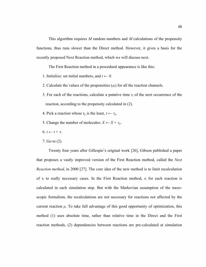
48
This algorithm requires M random numbers and M calculations of the propensity
functions, thus runs slower than the Direct method. However, it gives a basis for the
recently proposed Next Reaction method, which we will discuss next.
The First Reaction method in a procedural appearance is like this:
1. Initialize: set initial numbers, and t ← 0.
2. Calculate the values of the propensities (ai) for all the reaction channels.
3. For each of the reactions, calculate a putative time τi of the next occurrence of the
reaction, according to the propensity calculated in (2).
4. Pick a reaction whose τμ is the least, τ ← τμ.
5. Change the number of molecules: X ← X + τμ.
6. t ← t + τ.
7. Go to (2).
Twenty four years after Gillespie’s original work [26], Gibson published a paper
that proposes a vastly improved version of the First Reaction method, called the Next
Reaction method, in 2000 [27]. The core idea of the new method is to limit recalculation
of τl to really necessary cases. In the First Reaction method, τl for each reaction is
calculated in each simulation step. But with the Markovian assumption of the meso-
scopic formalism, the recalculations are not necessary for reactions not affected by the
current reaction μ. To take full advantage of this good opportunity of optimization, this
method (1) uses absolute time, rather than relative time in the Direct and the First
reaction methods, (2) dependencies between reactions are pre-calculated at simulation

49
start-up, and (3) the absolute putative time τl of each reaction is stored in a dynamic
priority queue data structure to speed up the operation of changing the value of τl.
The cost of this algorithm is just one random number generation and evaluations
of the propensity functions affected by the current reaction. This is supposed to be near or
perhaps on the theoretical limit as long as the simulation precisely tracks each occurrence
of reaction events. This method has to, however, maintain the priority queue, of which
cost is typically O(log2(M)) integer operations. Because the numbers of other operations
such as the random number generation and propensity function evaluations grows
proportionally to the density of the stoichiometry matrix, this logarithmic term can form a
bottleneck in computation speed for large Ms. The point of equilibrium between costs of
the priority queue and other operations is implementation and platform dependent. It is
worth noting, however, that recent advancements in pseudo random number generation
methods such as the Mersenne Twister algorithm [28] and integration of multiple high-
performance floating-point operation units into CPU chips have been lowering the
equilibrium point of M. Vasudeva and Bhalla [29] has some practical performance
comparisons of these methods.
Below are the step-by-step instructions for the Next Reaction method:
1. Initialize: set initial numbers, t ← 0, and for each reaction i, calculate a putative
time τi.
2. Pick the reaction with the least putative time τμ.
3. Change the number of molecules: X ← X + τμ.
4. t ← τμ.

50
5. for each affected reaction α,
(a) Calculate new aα, new.
(b) If α = μ, calculate new τα.
(c) If α ≠ μ,
tta
aa
new
olda )(
,
,
6. Go to 2.
The scaling operation in step 5(c) is an optimization to avoid using extra random
numbers, which is effectively equivalent as reusing the random numbers generated in the
previous step. Legitimacy of this random number reusing is discussed in detail in Gibson
and Bruck [27]. Of course, generating a new random number here and doing the same as
5(b) yields the same result.
To summarize, as long as the number of reactions is sufficiently large, and the
computation needs to be exact (each occurrence of a reaction must be counted), Gibson’s
Next Reaction method is the best known way of realizing simulation trajectories
according to CME.
Stochastic simulation methods also can be approximate using many possible ways.
Gillespie in 2001 [30] defined a simulation procedure called as tau-leaping method.
Continuously one of the best known approximate procedures is given in Gillespie and
Petzold [23] later.
2.3.4 Other methods

51
We reviewed some simulation methods in computational cell biology, and there
are several more schemes those are already in popular use or still under development.
Cellular automata (CA) is an important structure. The origin of CA traces back to
John von Neuman’s work [31] in theoretical computer science. Subsequently, it became a
major way of investigating qualitative simulations of complex phenomena in diffusion-
reaction systems, such as for excitable media and Turing patterns. Recently it is
becoming popular as a means of quantitative modeling and simulation of physical
phenomena such as fluid dynamics and diffusion-reaction [32]. Related to computational
cell biology is a type of CA for enzymatic reaction networks with spatial extent
represented by molecular diffusion proposed in Weimar [33]. Patel et al. [34] has an
application of CA to the model of tumor growth. Ermentrout and Edelstein-Keshet [35]
has some more references.
Another instance of a recent development is a hybrid dynamic/static pathway
simulation method that combines conventional ODE-based rate equations with static,
flux-based subcomponents [36]. The static part is based on a time-less metabolic flux
analysis (MFA), and its (re-)calculation is triggered by simulation steps of the dynamic,
ODE sub-components. Some more examples are Monte-Carlo Brownian dynamics
method originally developed for simulation of micro-scopic simulation of synaptic
transmission [37], boolean network, coupled map lattice, and difference equations.
This diversity in computational approaches is a natural consequence of the
heterogeneity and multiple scales of the cell as a dynamical system, and therefore is an

52
obvious reason of the need for the multi-formalism modeling and multi-algorithm
simulation discussed in the next section.
2.3.5 Multi-algorithm simulation
In the cell, as we have seen in the previous sections, various components with
different properties interact in diverse manners. All cellular subsystems are highly non-
linear, and couplings of the subsystems are often non-linear as well. The nonlinearity
indicates that the whole system is not equivalent to the sum of the subsystems. Although
a subsystem in isolation can be investigated to some extent by assuming steady and
simplified boundary conditions, the real behavior and role of the subsystem cannot be
elucidated unless it is considered as part of the whole.
Cell simulators must therefore allow simulation of cell subsystems in both
isolated and coupled forms. Simulation of coupled subsystems requires performing
computations on mutually interacting subsystems with different computational properties
on a single platform. There is, however, no universal algorithm which can efficiently
conduct simulation of all the subsystems at once, and so simulators must allow multiple
computation algorithms to coexist in a single model.
In order to support multi-algorithm computation, the scheme of the computing
must therefore provide a single abstract programming interface, which allows
indiscriminate interaction among the modules, and gives the front-end programs a
standard means of visualizing and manipulating these modules. This also means that the

53
implementations of the algorithm modules must be isolated from the system-provided
common interface.
Related to this necessity of the multi-algorithm simulator are the representation
schemes of the target physical entity (the cell) in the computer. The primary state
variables of a cell model are the quantities of species, and these can be modeled using
two different approaches. In the first, each state variable is a positive real number, and the
fractional parts are not discarded; this number format is suitable for working with the
empirical rate equations of biochemistry. The second approach keeps molecular
quantities as natural numbers, and a variety of methods may be used to maintain the
semantics of the fractional part, and these can be either stochastic or deterministic. In
addition, realistic cell models usually require a mixture of continuous state variables like
temperature, electric potential, and free energy, and discrete variables like the state flags
of multi-state molecules (e.g. transiently modified proteins). Therefore, the simulator
needs to handle types of positive, non-zero molecular quantities, real negative or positive
numbers, and discrete states of molecules.
As discussed design options, there are two design schemes of multi-formalism
simulation frameworks: embedding and combining approach.
A major source of strengths of the embedding approach is that it enforces
modularity, or context-independent design, on implemented modules. Each simulation
algorithm module and thus sub-model is required to have a well-defined interface of
time-scheduling and communications with other modules. Good outcomes of the
modularity of the embedding algorithm are:

54
• Once an algorithm is implemented in a modular way, it can be used in
combination with any other algorithm modules.
• Implementations of algorithm modules are often simpler and more maintainable
than combined forms of the same set of algorithms.
In fact, the embedding framework supports combining by allowing algorithms in
combined forms to be implemented as algorithm modules. Also the embedding
framework itself could be extended to support adaptive switching between algorithms by
providing a mechanism of ’Process migration’, which allows Process objects to migrate
among multiple Steppers of different algorithms during a simulation. This is one of our
future works.
On the other hand, one drawback in this modular design is that, because of the
inherent ’interface barriers’ between sub-models, dynamic switching between algorithms
implemented in different modules is still a future work, and currently not available. This
is immediately an advantage of the combined approach. For example, Gillespie’s tau-
leaping method can be viewed as a combination of an exact method and the approximate
tau-leaping scheme, and it switches to the exact method when the approximation
becomes inappropriate. These methods connect smoothly to each other in a natural way
as the scales of concentration and propensity changes.
Let’s take a closer look at this problem. A combination of two completely
different simulation algorithms treats different formalisms. An example is a combination
of a stochastic elementary reaction sub-model, for which Gillespie algorithm is often
used, and an ODE sub-model of Michaelis-Menten-type enzymatic complex reactions. In

55
a biochemical sense, these two sub-models require different types of kinetic parameters
and modeling approaches, and these are not inter-convertible. Another example is when
we have a model of metabolism as diffusion-reaction cellular automata, and want to co-
simulate this with a boolean-network model of gene expression. This case calls the
multiple modeling formalisms combined different simulation algorithms. Generally, this
approach only occasionally results in a good simulator design, as it requires a new
simulation algorithm to be developed for each distinct combination of modeling
formalisms, unless there is an existing algorithm generic enough to run these formalisms
simultaneously. Zeigler’s DEV&DESS [61] is an exceptionally useful example here,
because it combines two very general formalisms: discrete event and differential equation.
In this thesis we will introduce DEVS framework to solve system biological processes. In
the next chapter we will review some basic DEVS concepts, formalisms and the
implementation of the quantized integrator to Differential Equation models in
DEVSJAVA.
2.4 Existing software platforms and projects
Cell simulation is a relatively new area of computational science, but attempts to
numerically simulate biochemical pathways has a considerable history. This section
briefly reviews available software related to this work.
2.4.1 General purpose simulation software

56
One of the oldest publicly available software packages specialized for rate
equation based numerical simulation of cellular processes is KINSIM [38]. It is a DOS
application which is still actively used by biochemists for kinetic analysis of enzyme
reaction systems. GEPASI [39] is also a rate equation based simulator with an integrated
and easy to use interactive Windows GUI, and is widely used by biochemists for both
research and education. GEPASI’s successor, COPASI, is being developed with a focus
on large scalability and distributed parallel computing. DBSolve [40] is another ODE-
based simulator. ProMoT [41] is a Lisp based object-oriented modeling environment that
uses the DIVA numeric’s solver as a simulation backend. A commercial tool for block-
oriented generic simulation of complex systems, SCoP [42] is used to run differential and
difference equation based cell models. A-Cell [43] is a GUI-based piece of software used
to construct biochemical reactions and electro-physiological models of neurons and other
types of cell. Bio/Spice [44] was initially intended for genetic circuit simulation, and is
now being developed as a generic modeling and simulation environment linked to object-
relational databases. Jarnac, or SCAMP II, is a successor of the SCAMP simulator [45],
and equipped with a powerful and flexible scripting language that enables users to
program a dynamic object-oriented cell model. Virtual Cell [46] provides an intuitive
WWW Java applet based modeling environment which allows modelers to construct
spatial and biochemical models in both biological and mathematical semantic planes, and
has support for empirical 3D data from microscopy. PLAS [47] is a simple yet powerful
tool for modeling, simulation, and analysis of S-Systems. And still many groups use a

57
generic modeling package such as Mathematica or MatLab, although these tools are not
customized to support bio-simulation per se.
2.4.2 Specialized simulation software
StochSim [48] is a stochastic biochemical simulator in which individual
molecules and molecular complexes are represented as individual software objects. Its
unique algorithm makes for effective simulation of biochemical systems like the bacterial
chemotaxis signaling pathway, where only a small number of molecules are involved and
some of them are multi-state. MCell [37] is another simulator in which individual
molecules are treated not statistically, but individually, with a Monte-Carlo type random-
walk algorithm for Brownian dynamics. MCell is designed for the simulation of
interactions between ligands and binding sites on receptors, enzymes, and transporters
(amongst other molecules). Both simulators, StochSim and MCell, are somewhat
infrequently used for simulation of sub-cellular dynamics because of high computational
costs, yet the algorithms employed are likely to become indispensable if given
appropriate roles in a multi-algorithm whole cell model.
2.4.3 Software platforms and languages
The Caltech ERATO Kitano Systems Biology Project is developing an XML-
based Systems Biology Markup Language (SBML) as a means of interchanging bio-
simulation models [49]. The group has set out to encompass all the features of Bio/Spice,
DBSolve, E-Cell, Gepasi, Jarnac, StochSim, and Virtual Cell. A similar modeling

58
language being developed by the University of Auckland and Physiome Sciences is
CellML [50]. The Systems Biology Workbench (SBW) is also being developed by the
Caltech ERATO team [51]. SBW is a distributed object computing environment for
biological modeling and simulation. It provides an infrastructure that unifies various
software components like model editors, simulators and data analyzers/visualizers. Using
SBML as its language, it may well become the standard platform of model exchange,
data exchange, and inter-operation.
2.5 Systems Biology Markup Language
Systems biology is characterized by synergistic integration of theory,
computational modeling, and experiment [52]. Many contemporary research initiatives
demonstrate the growing popularity of this kind of multidisciplinary work (e.g. Abbott,
1999 [53]). There now exists a variety of computational tools for the budding systems
biologist (see below); however, the diversity of software has been accompanied by a
variety of incompatibilities, and this has lead to numerous problems. For example:
Users often need to work with complementary resources from multiple
simulation/analysis tools in the course of a project. Currently this involves
manually re-encoding the model in each tool, a time-consuming and error-prone
process.
When simulators are no longer supported, models developed in the old systems
can become stranded and unusable. This has already happened on a number of
occasions, with the resulting loss of usable models to the community. Continued

59
innovation and development of new software tools will only aggravate this
problem unless the issue is addressed.
Models published in peer-reviewed journals are often accompanied by
instructions for obtaining the model definitions. However, because each author
may use a different modeling environment (and model representation language),
such model definitions are often not straightforward to examine, test and reuse.
The current inability to exchange models between different simulation and
analysis tools has its roots in the lack of a common format for describing models. To
address this, a Software Platforms for Systems Biology forum under the auspices of the
ERATO Kitano Systems Biology Project was formed. The forum initially included
representatives from the teams developing the biological software packages.
The forum decided at the first meeting in April 2000 to develop a simple, XML-
based language for representing and exchanging models between simulation/analysis
tools: the Systems Biology Markup Language (SBML). They chose XML, the eXtensible
Markup Language [54], because of its portability and increasingly widespread acceptance
as a standard data language for bioinformatics [55]. SBML is formally defined using
UML, the Unified Modeling Language (Object Management Group, 2002), and this in
turn is used to define a representation in XML. The base definition, SBML Level 1[56], is
the result of analyzing common features in representation languages used by several
ODE-, DAE- and stochastic-based simulators, and encompasses the minimal information
required to support non-spatial biochemical models. Subsequent releases of SBML
(termed levels) will add additional structures and facilities to Level 1 based on features

60
requested and prioritized by the SBML community. By freezing sets of features in SBML
definitions at incremental levels, they hope to provide software authors with stable
standards and allow the simulation community to gain experience with the language
definitions before introducing new elements.
2.5.1 Structure of Model Definitions in SBML
A chemical reaction can be broken down into a number of conceptual elements:
reactant species, product species, reactions, stoichiometries, rate laws, and parameters in
the rate laws. To analyze or simulate a network of reactions, additional components must
be made explicit, including compartments for the species, and units on the various
quantities. A definition of a model in SBML simply consists of lists of one or more of
these various components (Figure 2.2, Figure 2.3):
Figure 2.2 an SBML Document Structured
Figure 2.3 a model according to SBML

61
Compartment: A container of finite volume for well-stirred substances where reactions
take place.
Species: A chemical substance or entity that takes part in a reaction. Some example
species are ions such as calcium ions and molecules such as ATP.
Reaction: A statement describing some transformation, transport or binding process that
can change one or more species. Reactions have associated rate laws describing
the manner in which they take place (Figure 2.4).
Parameter: A quantity that has a symbolic name. SBML provides the ability to define
parameters that are global to a model, as well as parameters that are local to a
single reaction.
Unit definition: A name for a unit used in the expression of quantities in a model. This is
a facility for both setting default units and for allowing combinations of units to
be given abbreviated names.
Rule: A mathematical expression that is added to the model equations constructed from
the set of reactions. Rules can be used to set parameter values, establish
constraints between quantities, etc.
Function: A named mathematical function that may be used throughout the rest of a
model.
Event: A statement describing an instantaneous, discontinuous change in a set of
variables of any type (species quantity, compartment size or parameter value)
when a triggering condition is satisfied.
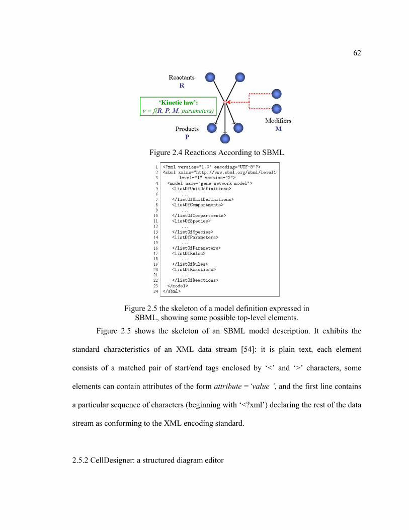
62
Figure 2.4 Reactions According to SBML
Figure 2.5 the skeleton of a model definition expressed in SBML, showing some possible top-level elements.
Figure 2.5 shows the skeleton of an SBML model description. It exhibits the
standard characteristics of an XML data stream [54]: it is plain text, each element
consists of a matched pair of start/end tags enclosed by ‘<’ and ‘>’ characters, some
elements can contain attributes of the form attribute =‘value ’, and the first line contains
a particular sequence of characters (beginning with ‘<?xml’) declaring the rest of the data
stream as conforming to the XML encoding standard.
2.5.2 CellDesigner: a structured diagram editor

63
CellDesigner [57] is a structured diagram editor for drawing gene-regulatory and
biochemical networks. Networks are drawn based on the process diagram, with graphical
notation system proposed by Kitano [52], and are stored using SBML, a standard for
representing models of biochemical and gene-regulatory networks.
Figure 2.6 the user interface of CellDesigner ver.3.5.2
2.5.3 LibSBML
LibSBML [58] is a library designed to help you read, write, manipulate, translate,
and validate SBML files and data streams. It is not an application itself (though it does
come with many example programs), but rather a library you can embed in your own
applications.
LibSBML is written in ISO C and C++ but as a library it may be used from all the
programming languages C++, C, Java, Python, Perl, Lisp, Matlab, and Octave. In fact,
they strive to adhere to the natural idioms of each particular language to make the

64
libSBML programming experience seamless. For example, SBML <listOf> elements
behave like lists and sequences in Python, but vectors in Matlab. Also, the C and C++
interfaces are completely distinct (it's possible to program in pure C), but in C++ the C
APIs may be called without sacrificing type safety.
The LibSBML code is very portable and is supported on Linux, Windows (native),
and Mac OS X.

65
CHAPTER 3 DEVS AND DEVSJAVA
In this chapter, firstly we review some basic DEVS concepts, formalisms and
algorithms. Secondly Multi-algorithm framework and Differential Equation models were
introduced. And lastly the implementation of the Quantized integrator to Differential
Equations was given in DEVSJAVA.
3.1 DEVS
3.1.1 DEVS and DEVS Formalism
Discrete Event System Specification (DEVS) is a mathematical formalism to
describe real-world system behavior in an abstract and rigorous manner. Compared with
traditional methodology for modeling and simulation, DEVS formalism describes and
specifies a modeled system as a mathematical object, and such object based
representation of the targeted system can then be implemented using different simulation
languages, especially modern object-oriented ones. In general, a system has a set of key
parameters when being modeled in a modeling framework, which include time base,
inputs, states, outputs, and functions for determining state transitions. Discrete event
systems in general encapsulate these parameters as object entities, and then use modern
object oriented simulation languages to describe the relationship among the specified
entities. As a pioneering formal modeling and simulation methodology, DEVS provides a

66
concrete simulation theoretical foundation, which promotes fully object-oriented
modeling and simulation techniques for solving today’s simulation problems required by
other science and engineering discipline. The insight provided by the DEVS formalism is
in the simple way that it characterizes how discrete event simulation languages specify
discrete event system parameters [59]. Having such an abstraction, it is possible to design
new simulation languages with sound semantics that are easier to understand than
traditional ones. Figure 3.1 presents a DEVS concept framework to show the basic
objects and their relationships in a DEVS modeling and simulation world. These basic
objects include [60]:
• The real system, in existence or proposed, which is regarded as fundamentally a
source of data
• model, which is a set of instructions for generating data comparable to that
observable in the real system. The structure of the model is its set of instructions. The
behavior of the model is the set of all possible data that can be generated by faithfully
executing the model instructions.
• simulator, which exercises the model's instructions to actually generate its behavior.
• experimental frame, which captures how the modeler’s objectives impact on model
construction, experimentation and validation. As implemented in DEVSJAVA, such
experimental frames are formulated as model objects in the same manner as the
models of primary interest. In this way, model/experimental frame pair’s form
coupled model objects with the same properties as other objects of this kind. It will

67
become evident later, that this uniform treatment yields immediate benefits in terms
of modularity and system entity structure representation.
These basic objects are then related by two relations [60]:
• modeling relation: linking real system and model, defines how well the model
represents the system or entity being modeled. In general terms a model can be
considered valid if the data generated by the model agrees with the data produced by
the real system in an experimental frame of interest.
• simulation relation, linking model and simulator, represents how faithfully the
simulator is able to carry out the instructions of the model.
Figure 3.1 Basic Entities and Relations [60]
In the view from DEVS, the basic items of data produced by a system or model
are time segments. These time segments are mappings from intervals defined over a
specified time base to values in the ranges of one or more variables [60]. These variables
can either be observed or measured. An example of a data segment is shown in Figure 3.2,
where X is inputs, S is states, e is time elapsed, and Y is outputs.

68
In fact, DEVS formalism provides a formal definition to describe the data
segment depicted above in Figure 3.2, and the history of DEVS can be traced back to
decades ago.
Figure 3.2 Discrete Event Time Segments [61]
A standard and classic DEVS formalism is defined as a structure [61]:
DEVS = (X, Y, S, ext, int, , ta)
Where
X is the set of inputs;
Y is the set of outputs;
S is the set of sequential states;
ext: Q X S is the external state transition function;
int: S S is the internal state transition function;
: S Y is the output function;
ta: S is the time advance function;
With Q = (s, e) | s S, 0≤ e ≤ ta(s) is the set of total states.

69
Figure 3.3 illustrates the key concept of above classic DEVS formalism. Assuming
the system is in state S after a previous state transition, it will stay in state S for a duration
determined by ta(s). When this resting time of ta() expires (or say the elapsed time
e=ta(s)), the system gives output (s) and changes its state from s to s’. This state
transition is exactly determined by the internal transition function int as mentioned in
the formalism. However, if an external event occurs through the input X before the
duration specified by ta(s) (or say, the system is in total state (s, e) with e = ta(s), the
system will change to a state determined by ext (s, e, x). After the system changes its
state to a new state, the same rules in the formalism are applied to govern how the system
responses to discrete events. DEVS makes an explicit difference between internal and
external state transitions, where the internal transition function determines the system’s
new state when no events have occurred since the last transition, while the external
transition function determines the system’s new state when an external event occurs
between 0 and ta(s). It is worth to note that ta(s) is a real number including 0 and, where
“0” means that the system is a so-called “transitory” state that no external events can
intervene, and “” means that the system is in a so-called “passive” state that is
unchanged forever until an external event wakes it up.

70
Figure 3.3 an Illustration for Classic DEVS Formalism [61]
The above classic DEVS formalism does not take into account of concurrent
events, and therefore, has relatively limited usage for real-world application. With the
consideration of concurrent events and parallel processing on a discrete event system,
parallel DEVS system specification is developed from classic DEVS. The key
capabilities of Parallel DEVS beyond the classical DEVS are [61]:
Ports are represented explicitly – there can be any of input and output ports on
which values can be received and sent.
Instead of receiving a single input or sending a single output, basic parallel DEVS
models can handle bags of inputs and outputs. It should be noted here that a bag
can contain many elements with possibly multiple occurrences of its elements.
A transition function, called confluent, is added, which decides the next state in
cases of collision between external and internal events.
Such parallel DEVS formalism consists of two parts: basic and coupled models. A
basic model of a standard parallel DEVS is a structure [61]:
DEVS = (X, Y, S, ext, int, con, ta)
With X is the set of input events;

71
S is the set of sequential states;
Y is the set of output events;
int: S S is the internal transition function;
ext: Q x Xb S is the external transition function,
Where Xb is a set of bags over elements in X,
con: S x Xb S is the confluent transition function,
Subject to con(s, ) = int(s)
: S Yb is the output function;
ta: S is the time advance function,
Where Q = (s, e) s S, 0 < e < ta(s), and e is the elapsed time since
last state transition.
Such basic model as defined in parallel DEVS captures the following information
from a discrete event system:
the set of input ports through which external events are received
the set of output ports through which external events are sent
the set of state variables and parameters
the time advance function which controls the timing of internal transitions
the internal transition function which specifies to which next state
the system will transit after the time given by the time advance function has
elapsed

72
the external transition function which specifies how the system changes state when
an input is received. The next state is computed on the basis of the present state,
the input port and value of the external event, and the time that has elapsed in the
current state
the confluent transition function which decides the next state in cases of collision
between internal and external events
the output function which generates an external output just before an internal
transition takes place
Basic model is a building block for a more complex coupled model, which defines
a new model constructed by connecting basic model components. Two major activities
involved in coupled models are specifying its component models and defining the
couplings which create the desired communication networks. A coupled model is defined
as follows [61]:
DN = <X, Y, D, Mi, Ii, Zi,j>
Where X is a set of external input events;
Y is a set of outputs;
D is a set of components names;
for each i in D,
Mi is a component model
Ii is the set of influences for i
for each j in Ii,
Zi,j is the i-to-j output translation function

73
A coupled model template captures the following information:
the set of components
for each component, its influences
the set of input ports through which external events are received
the set of output ports through which external events are sent
the coupling specification consisting of:
the external input coupling (EIC) connects the input ports of the coupled to
one or more of the input ports of the components
the external output coupling (EOC) connects the output ports of the
components to one or more of the output ports of the coupled model
internal coupling (IC) connects output ports of components to input ports of
other components
As we have seen in this section, DEVS formalisms are strictly defined and it
evolves continuously to satisfy the requirement of today’s large and complex system
modeling and simulation. It has been extended by a lot of researcher around world;
however, its core concept is unchanged as we can see from the classic and parallel
formalisms. In the next section, we will discuss DEVS modeling framework.
3.1.2 Basic systems modeling formalisms
The basic systems modeling formalisms can be classified into three categories:
Differential Equation System Specifications (DESS), Discrete Time System
Specifications (DTSS), and Discrete Event System Specifications (DEVS) (Figure 3.4)

74
[61]. However, many real world phenomenons cannot be fit into the Procrustean bed of
one formalism at a time. More generally, the ambitious systems now being designed,
such as an automated highway traffic control system, cannot be modeled by a pure
discrete or continuous paradigm. Instead, they require a combined discrete/continuous
modeling and simulation methodology that supports a multi-formalism modeling
approach and the simulation environments to support it.
Figure 3.4 Basic Systems Specification Formalisms
3.1.3 Multi-algorithm framework
Skipping many years of accumulating developments, the next major advance in
systems formalisms was the combination of discrete event and differential equation
formalisms into one, the DEV&DESS. This formalism subsumes both the DESS and the
DEVS and thus supports the development of coupled systems whose components are
expressed in any of the basic formalisms. Such multi-formalism modeling capability is
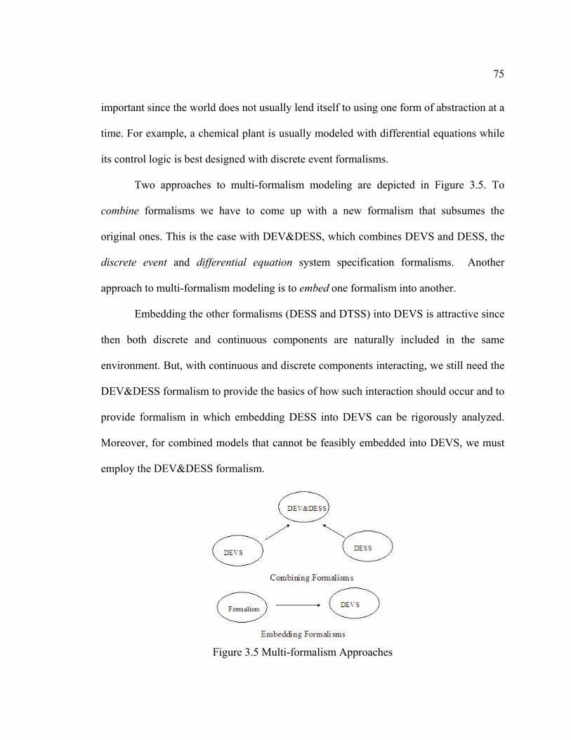
75
important since the world does not usually lend itself to using one form of abstraction at a
time. For example, a chemical plant is usually modeled with differential equations while
its control logic is best designed with discrete event formalisms.
Two approaches to multi-formalism modeling are depicted in Figure 3.5. To
combine formalisms we have to come up with a new formalism that subsumes the
original ones. This is the case with DEV&DESS, which combines DEVS and DESS, the
discrete event and differential equation system specification formalisms. Another
approach to multi-formalism modeling is to embed one formalism into another.
Embedding the other formalisms (DESS and DTSS) into DEVS is attractive since
then both discrete and continuous components are naturally included in the same
environment. But, with continuous and discrete components interacting, we still need the
DEV&DESS formalism to provide the basics of how such interaction should occur and to
provide formalism in which embedding DESS into DEVS can be rigorously analyzed.
Moreover, for combined models that cannot be feasibly embedded into DEVS, we must
employ the DEV&DESS formalism.
Figure 3.5 Multi-formalism Approaches
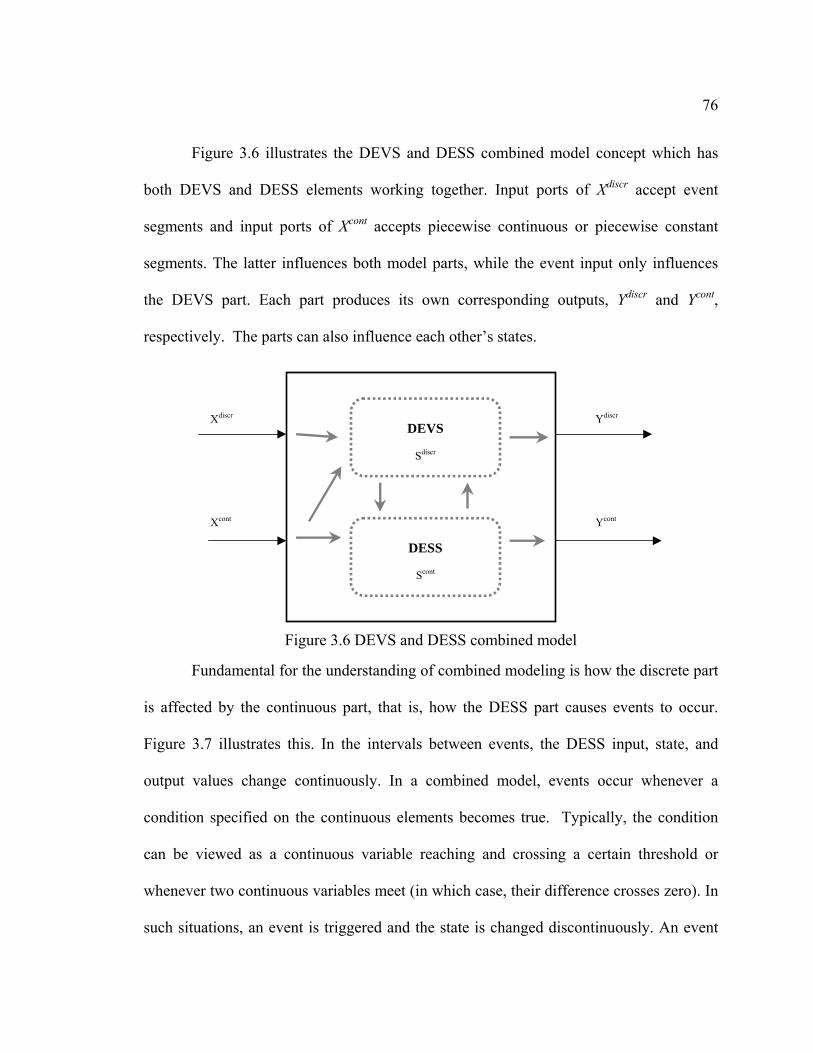
76
Figure 3.6 illustrates the DEVS and DESS combined model concept which has
both DEVS and DESS elements working together. Input ports of Xdiscr accept event
segments and input ports of Xcont accepts piecewise continuous or piecewise constant
segments. The latter influences both model parts, while the event input only influences
the DEVS part. Each part produces its own corresponding outputs, Ydiscr and Ycont,
respectively. The parts can also influence each other’s states.
DEVS
Sdiscr
DESS
Scont
Xdiscr
Xcont Ycont
Ydiscr
Figure 3.6 DEVS and DESS combined model
Fundamental for the understanding of combined modeling is how the discrete part
is affected by the continuous part, that is, how the DESS part causes events to occur.
Figure 3.7 illustrates this. In the intervals between events, the DESS input, state, and
output values change continuously. In a combined model, events occur whenever a
condition specified on the continuous elements becomes true. Typically, the condition
can be viewed as a continuous variable reaching and crossing a certain threshold or
whenever two continuous variables meet (in which case, their difference crosses zero). In
such situations, an event is triggered and the state is changed discontinuously. An event

77
which is caused by the changes of continuous variables is called a state event (in
distinction to internal events of pure DEVS which are scheduled in time and are called
time events).
state event
scont
threshold
t T
threshold reached
discrete change
Figure 3.7 state event
In the subsequent section, DEVSJAVA, a known implementation of parallel
DEVS formalism, is reviewed with the focus on how to solve the Differential Equation
using DEVS view.
3.2 Differential Equation Models
Recall that in discrete time modeling there is a state transition function which
computes the state at the next time instant given the current state and input. In the
classical modeling approach of differential equations, the state transition relation is quite
different. For differential equation models we do not specify a next state directly but
instead, use a derivative function to specify the rate of change of the state variables. At
any particular time instant on the time axis, given a state and an input value, we only
know the rate of change of the state. The state at any point in the future must compute
from this information.

78
3.2.1 Basic Model: The Integrator
To see how this form of modeling works, let us consider the most elementary
continuous system – the simple integrator (Figure 3.8). The integrator has one input
variable x and one output variable y. One can imagine it as a reservoir with infinite
capacity. Whatever is put into the reservoir is accumulated – with a negative input value
meaning outflow. The state of the reservoir is its current contents. When we want to
express this in equation form we need a variable to represent the current contents. This is
our state variable q. The current input x represents the rate of current change of the
contents which we express by equation
dq(t) / dt = x(t)
and the output y is equal to the current state
y(t) = q(t)
x
x(t)
y
t
x(t)y(t)
input
contents = input dt
Figure 3.8 Basic Integrator Concepts
Usually continuous systems are expressed by using several state variables.
Derivatives are then functions of some, or all, the state variables. Let q1, q2, ..., qn be the

79
state variables and x1, x2, ..., xm be the input variables, and then a continuous model is
formed by a set of first-order differential equations
d q1(t)/dt = f1(q1(t), q2(t), ..., qn(t), x1(t), x2(t), ..., xm(t))
d q2(t)/dt = f2(q1(t), q2(t), ..., qn(t), x1(t), x2(t), ..., xm(t))
...
d qn(t)/dt = fn(q1(t), q2(t), ..., qn(t), x1(t), x2(t),..., xm(t))
Figure 3.9 the Integrator
Note that the derivatives of the state variables qi are computed respectively, by
functions fi which have the state and input vectors as arguments. Representing the
integrator in diagrammatic form as in Figure 3.10, we can represent a set of first order
differential equations in the coupled model form of Figure 3.10. The state and input
vector are input to the rate of change functions fi. Those provide as output the derivatives
dqi/dt of the state variables qi which are forwarded to integrator blocks. The outputs of
the integrator blocks are the state variables qi.
d q1/dt q1f1x
d q2/dt q2f2
d qn/dt qnfn
qx
qx
qx
...
Figure 3.10 Structure of differential equation specified systems

80
3.2.2 Continuous system simulation
The diagram above reveals the fundamental problem that occurs when a
continuous system is simulated on a digital computer. In the diagram we see that given a
state vector q and an input vector x for a particular time instant ti we only obtain the
derivatives dqi/dt. But how do we obtain the dynamic behavior of the system over time?
In other words, how do we obtain the state values after this time? This problem is
depicted in Figure 3.11. In digital simulation, there is necessarily a next computation
instant ti+1 and a nonzero interval [ti, ti+1]. The model is supposed to be operating in
continuous time over this interval, and the input, state and output variables change
continuously during this period. The computer program has available only the values at ti
and from those it must estimate the values at ti+1 without knowledge of what is happening
in the gaps between ti and ti+1. This means it must do the calculation without having
computed the input, state, and output trajectories associated with the interval (ti, ti+1).
1
f(s(ti),x(ti))
x(ti)
q
x
q(ti)
Figure 3.11 Continuous system simulation problems
Schemes for solving this problem are generally known as numerical integration
methods. A whole literature deals with design and analysis of such methods [62] [63].

81
The basic idea of numerical integration is easily stated an integration method
employs estimated past and/or future values of states, inputs and derivatives in an effort
to better estimate a value for the present time ( 0) (Figure 3.12). Thus to compute a state
value q(ti) for a present time instance ti, may involve computed values of states, inputs
and derivatives at prior computation times ti-1, ti-2, ... and/or predicted values for the
current time ti and subsequent time instants ti+1, ti+2, ...
Notice that the values of the states and the derivatives are mutually interdependent
– the integrator itself causes a dependence of the states on the derivatives and through the
derivative functions fi the derivatives are dependent on the states. This situation sets up an
inherent difficulty which must be faced by every approximation method - the propagation
of errors.
q
x
q(ti)
titi-1ti-2 ti+1 ti+2
Figure 3.12 Computing state values at time ti based on estimated values at time instants prior and past time ti
We consider the simplest integration method, generally known as the Euler or
rectangular method. The idea underlying the Euler method is that for a perfect integrator
h
tqhtq
dt
tdqh
)()(lim
)(0
thus for small enough h, we should be able to use the approximation

82
dt
tdqhtqhtq
)()()(
Now the input to an integrator, as in Figure 3.9, is the derivative x(t) = dq/dt. So we have
q(t+h) = q(t) + h x(t)
With h fixed, we can iterate to compute successive states at time instants 0, h, 2h, 3h, …
given the initial state at time 0 and the input values x(0), x(h), … Although
straightforward to apply, Euler integration has some drawbacks. On one hand, to obtain
accurate results the step size h has to be sufficiently small. But the smaller the step size
the more iterations are needed and hence the greater the computation time for a given
length of run. On the other hand the step size also cannot be decreased indefinitely, since
the finite word size of digital computers introduces round-off and truncation errors.
Therefore, a host of different integration method have been developed which often show
much better speed/accuracy tradeoffs than the simple Euler method. However, these
methods introduce stability problems as we discuss in a moment.
We now describe briefly the principles of some frequently employed integration
methods. We can distinguish methods according to whether or not they use estimated
future values of variables to compute the present values. We call a method causal if it
only employs values at prior computation instants. A method is called non-causal if in
addition to prior values it also employs estimated values at time instants at and after the
present time. The order of a method is the number of pairs of derivative/state values it
employs to compute the value of the state at time ti. For example, a method employing

83
the values of q and its derivative at times ti-2, ti-1, ti, and ti+1 are of order 4. Table 3.1
summarizes the pros and cons of integration methods.
Table 3.1 Summary of Integration Method Speed-Accuracy Tradeoffs
Integration Method
Efficiency Start-up Problems Stability Problems Robustness
Euler low none not for sufficiently small step sizes
high
Causal methods high yes yes low Non-Causal methods
high no, if only future values used
yes low
3.3 Differential Equation Models in DEVSJAVA
3.3.1 DEVSJAVA
DEVSJAVA [64] is an implementation in Java of DEVS framework that has been
used for solving real-world simulation problem as well as serving as an openly available
teaching tool. It is a fully object orient implementation of standard parallel DEVS
formalism, and therefore, provides a very dynamic and flexible modeling and simulation
framework. DEVSJAVA has relatively complex class hierarchical structure. The base
classes of the DEVS sub-hierarchy are Atomic and Coupled as the main derived classes of
it [64]. Class digraph is a main subclass of class coupled to define coupled model as
described in previous subsection. For DEVS model developers, the user-defined model
classes should derive from these basic classes and such model classes then become new
components in DEVS for later reuse. The implementation of DEVSJAVA supports the
fundamental concept of DEVS hierarchical construction and makes it easier to build
complex model.

84
3.3.2 DEVS representation of discrete event integrators
It is useful to have a compact representation of the integration scheme that is
readily implemented on a computer, can be extended to produce new schemes, and
provides an immediate support for parallel computing. DEVS satisfies this need. A
detailed treatment of DEVS can be found in [61]. Several simulation environments for
DEVS are readily available online (e.g. PowerDEVS [65], adevs [66], DEVSJAVA [67],
CD++ [68], and JDEVS [69] to name just a few).
DEVS uses two types of structures to describe a discrete event system. Atomic
models describe the behavior of elementary components. Here, an atomic model will be
used to represent individual integrators and differential functions. Coupled models
describe collections of interacting components, where components can be atomic and
coupled models. In this application, a coupled model describes a system of equations as
interacting integrators and function blocks.
An atomic model is described by a set of inputs, set of outputs, and set of states, a
state transition function decomposed into three parts, an output function, and a time
advance function. Formally, the structure sees the basic model of a standard parallel
DEVS in section 3.1.1. The external transition function describes how the system
changes state in response to input. When input is applied to the system, it is said that an
external event has occurred. The internal transition function describes the autonomous
behavior of the system. When the system changes state autonomously, an internal event
is said to have occurred. The confluent transition function determines the next state of the

85
system when an internal event and external event coincide. The output function generates
output values at times that coincide with internal events. The output values are
determined by the state of the system just prior to the internal event. The time advance
function determines the amount of time that must elapse before the next internal event
will occur, assuming that no input arrives in the interim.
Coupled models are described by a set of components and a set of component
output to input mappings. For our purpose, we can restrict the coupled model description
to a flat structure (i.e., a structure composed entirely of atomic models) without external
input or output coupling (i.e., the component models can not be affected by elements
outside of the network). With these restrictions, a coupled model is described by the
structure
N =< Mk, zij >
Where
Mk is a set of atomic models, and
zij is a set of output to input maps zij: Yi Xj Φ
Where the i and j indices correspond to Mi and Mj in Mk and Φ is the non-event:
The output to input maps describe which atomic models can affect one another.
The output to input map is, in this application, somewhat over generalized and could be
replaced with more conventional descriptions of computational stencils and block
diagrams. The non-event is used, in this instance, to represent components that are not
connected. That is, if component i does not influence component j, then zij (xi) = Φ, where
xi Xi.

86
These structures describe what a model can do. A canonical simulation algorithm
is used to generate dynamic behavior from the description. The algorithm is given in the
following DEVS algorithm. Algorithm assumes a coupled model N, with a component set
M1, M2,…, Mn, and a suitable set of output to input maps. For every component model
Mi, there is a time of last event and time of next event variable tLi and tNi, respectively.
There are also state, input, and output variables si, xi, and yi, in addition to the basic
structural elements (i.e., state transition functions, output function, and time advance
function). The variables xi and yi are bags, with elements taken from the input and output
sets Xi and Yi, respectively. The simulation time is kept in variable t.
Each of the x variables is associated with an atomic model called an integrator.
The input to the integrator is the value of the differential function, and the output of the
integrator is the appropriate y variable. The integrator has four state variables
ql, the last output value of the integrator,
q, the current value of the integral,
dq/dt, the last known value of the derivative, and
σ, the time until the next output event.
The integrator's input and output events are real numbers. The value of an input
event is the derivative at the time of the event. An output event gives the value of the
integral at the time of the output.
DEVS simulation algorithm
t ← 0 Initialize the models

87
for all i [1, n] do
tLi ← 0
set si to the initial state of Mi
end for
while terminating condition not met do
for all i [1, n] do
tNi ← tLi + ta(si)
Empty the bags xi and yi
end for
t ← mintNi
for all i [1, n] do
if tNi = t then
yi ←i(si)
for all j [1, n] & j ≠ i & zij (yi) ≠ do
Add zij (yi) to the bag xj
end for
end if
end for
for all i [1, n] do
if tNi = t & xi is empty then
si ← int,i(si)
tLi ← t

88
else if tNi = t & xi is not empty then
si ← con,i(si, xi)
tLi ← t
else if tNi ≠ t & xi is not empty then
si ← ext,i(si,t – tLi,xi)
tLi ← t
end if
end for
end while
3.3.3 Mapping Differential Equation Models into DEVS Integrator Models
Figure 3.13 shows the mapping Differential Equation Systems to DEVS
Simulators in DEVSJAVA Simulation of Continuous Systems.
Figure 3.13 Mapping Differential Equation Models into DEVS Integrator Models

89
3.3.4 DEVS Representation of Quantized Integrator in DEVSJAVA
The DEVS realization of the quantized integrator has the simple definition:
M = (X, Y, S, ext, extint, , ta).
Where X = Y = R, S = R R I and
ext((q, x, n), e, x’) = (q + x*e, x’, n)
int(q, x, n) = (n + D*sign(x), x, n + sign(x) )
con((q, x, n), x’) = (n + D*sign(x), x’, n + sign(x))
(q, x) = (n + sign(x))*D
ta(q, x, n) = | ((n+1)D - q)/x | if x > 0 and (n+1)D - q > 0
= | (q - nD)/x | if x < 0 and if |q-nD| > 0
= | D/x | if x 0 and none of the above
= otherwise (i.e., x = 0)
Here we keep track of the boundary below (or at) the current state q, i.e, the
integer floor (q/D). Recall that even if we start on a boundary, the state may eventually
be inside a block (hence not a multiple of D) as a result of an external transition. If, as in
Figure 3.14(a), we are on a boundary, the time advance computation merely divides D by
the current input x (which is the derivative, or slope, after all). If we reach the upper
boundary (n+1) or lower boundary (n–1), we output and update the state accordingly.
Note that so long as the input remains the same, the time to cross successive boundaries
will be the same. Figure 3.14 (b) shows that when a new input is received, we update the

90
state using the old input and the elapsed time. From this new state, q, the new time to
reach either the upper or lower boundary is computed.
The Quantized DEVS integrator greatly reduces the number of transitions and
output messages needed to simulate an integrator. It also reduces the message size from
double to integer. Actually since the only possible transitions are to the upper or lower
boundaries, only one bit to represent the binary valued set +1, -1 need be sent.
Figure 3.14 DEVS simulator of a Quantized Integrator
The implementation of the Quantized Integrator and Instantaneous Functions is
given in DEVSJAVA Continuous package [70].

91
CHAPTER 4 DEVS COMBINED WITH SBML SYSTEM IN
CELL BIOLOGY
In the previous chapters, an implication of the ’ontological complexity’ of the cell
that leads to need for a sophisticated software platform has been discussed. Unlike some
of conventional approaches to physical and biochemical systems, such complicated
nature of the cell as a target system is inevitably reflected by the design and
implementation of the software.
In this chapter, we introduce a new technique DEVS to solve the Cell Biology
Processes. We will discuss design and implementation of DEVS-SBML Platform, a new
simulation platform based on DEVS and SBML to enable sharing of biological models.
This platform will be compatible DEVS model with SBML model to solve Biology
Processes using DEVS ODE solver. We put an emphasis on architecture and
implementation of DEVS-SBML Simulation Platform, a part of the DEVS-SBML
Platform of which core is an object-oriented simulation engine that implements the cell
simulation using DEVS algorithm discussed in the previous chapter.
4.1 Introduction
Computational cell biology is a rapidly growing simulation-oriented research field
that has been greatly stimulated by the array of high throughput methods developed in
recent years. In a previous chapter, we have argued that cell simulation poses many
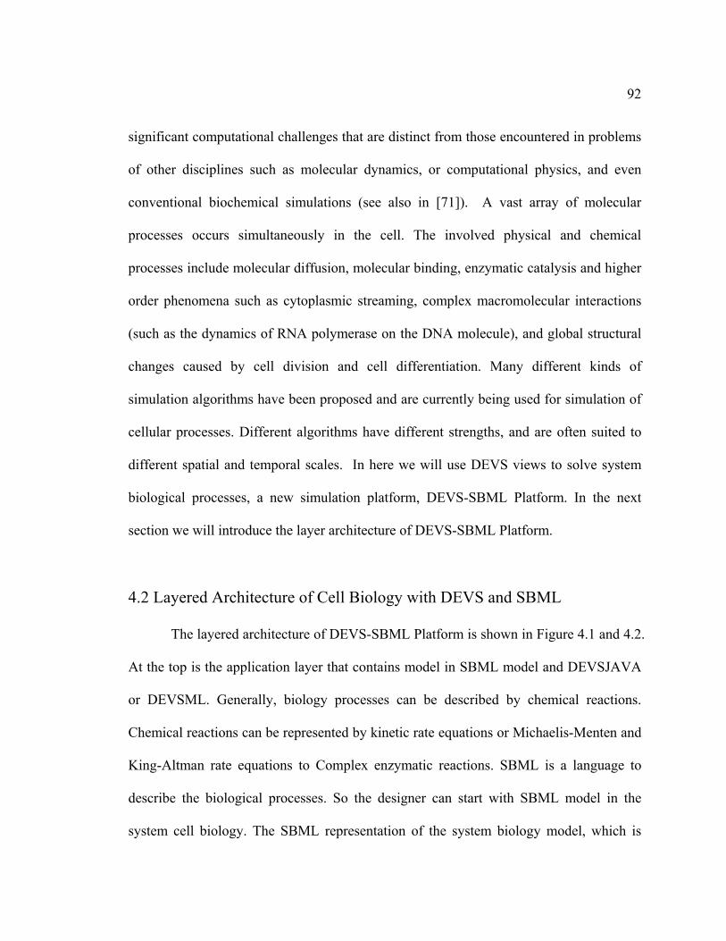
92
significant computational challenges that are distinct from those encountered in problems
of other disciplines such as molecular dynamics, or computational physics, and even
conventional biochemical simulations (see also in [71]). A vast array of molecular
processes occurs simultaneously in the cell. The involved physical and chemical
processes include molecular diffusion, molecular binding, enzymatic catalysis and higher
order phenomena such as cytoplasmic streaming, complex macromolecular interactions
(such as the dynamics of RNA polymerase on the DNA molecule), and global structural
changes caused by cell division and cell differentiation. Many different kinds of
simulation algorithms have been proposed and are currently being used for simulation of
cellular processes. Different algorithms have different strengths, and are often suited to
different spatial and temporal scales. In here we will use DEVS views to solve system
biological processes, a new simulation platform, DEVS-SBML Platform. In the next
section we will introduce the layer architecture of DEVS-SBML Platform.
4.2 Layered Architecture of Cell Biology with DEVS and SBML
The layered architecture of DEVS-SBML Platform is shown in Figure 4.1 and 4.2.
At the top is the application layer that contains model in SBML model and DEVSJAVA
or DEVSML. Generally, biology processes can be described by chemical reactions.
Chemical reactions can be represented by kinetic rate equations or Michaelis-Menten and
King-Altman rate equations to Complex enzymatic reactions. SBML is a language to
describe the biological processes. So the designer can start with SBML model in the
system cell biology. The SBML representation of the system biology model, which is
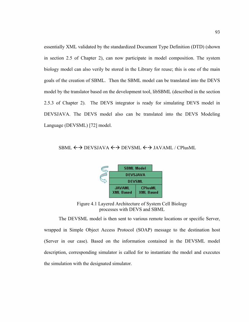
93
essentially XML validated by the standardized Document Type Definition (DTD) (shown
in section 2.5 of Chapter 2), can now participate in model composition. The system
biology model can also verily be stored in the Library for reuse; this is one of the main
goals of the creation of SBML. Then the SBML model can be translated into the DEVS
model by the translator based on the development tool, libSBML (described in the section
2.5.3 of Chapter 2). The DEVS integrator is ready for simulating DEVS model in
DEVSJAVA. The DEVS model also can be translated into the DEVS Modeling
Language (DEVSML) [72] model.
SBML DEVSJAVA DEVSML JAVAML / CPlusML
Figure 4.1 Layered Architecture of System Cell Biology
processes with DEVS and SBML
The DEVSML model is then sent to various remote locations or specific Server,
wrapped in Simple Object Access Protocol (SOAP) message to the destination host
(Server in our case). Based on the information contained in the DEVSML model
description, corresponding simulator is called for to instantiate the model and executes
the simulation with the designated simulator.

94
Figure 4.2 the Architecture of System Cell Biology processes with DEVS and SBML
DEVSML
The second layer is the DEVSML layer itself that provides seamless integration,
composition and dynamic scenario construction resulting in portable models in DEVSML
that are complete in every respect. These DEVSML models can be ported to any remote
location using the net-centric infrastructure and be executed at any remote location.
Another major advantage of such capability is total simulator ‘transparency’. The
simulation engine is totally transparent to model execution over the net-centric
infrastructure. The DEVSML model description files in XML contains meta-data
information about its compliance with various simulation ‘builds’ or versions to provide
true interoperability between various simulator engine implementations. This has been
achieved for at least two independent simulation engines as they have an underlying
DEVS protocol to adhere to. This has been made possible with the implementation of a

95
single atomic DTD and a single coupled DTD that validates the DEVSML descriptions
generated from these two implementations. Such run-time interoperability provides great
advantage when models from different repositories are used to compose bigger coupled
models using DEVSML seamless integration capabilities.
JavaML / CPlusML
JavaML [73] is an XML-Based source code representation for Java programs. The
JAVAML DTD specifies various elements of a valid JavaML document. It is well-suited
to be used as canonical representation of Java source code for tools. It comes with an
XSLT-based back-converter that translates a JavaML document back into java source
code. More details about JavaML can be found at [73]. CPlusML also is an XML-Based
source code representation for C++ programs. CPlusML is still under development.
4.3 DEVS with SBML Platform
We want to develop a platform for the DEVS with SBML (DEVS-SBML) to
model and simulate biological processes. Through this modeling and simulation platform,
we hope to increase the productivity of biologists.
4.3.1 DEVS-SBML Platform
DEVS-SBML Platform is a chemical kinetics simulation software platform
implemented in Java. It provides a model definition environment and various simulation
engines for evolving a dynamical model from specified initial data. A model consists of a
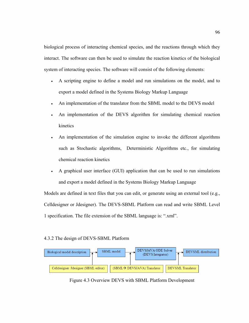
96
biological process of interacting chemical species, and the reactions through which they
interact. The software can then be used to simulate the reaction kinetics of the biological
system of interacting species. The software will consist of the following elements:
A scripting engine to define a model and run simulations on the model, and to
export a model defined in the Systems Biology Markup Language
An implementation of the translator from the SBML model to the DEVS model
An implementation of the DEVS algorithm for simulating chemical reaction
kinetics
An implementation of the simulation engine to invoke the different algorithms
such as Stochastic algorithms, Deterministic Algorithms etc., for simulating
chemical reaction kinetics
A graphical user interface (GUI) application that can be used to run simulations
and export a model defined in the Systems Biology Markup Language
Models are defined in text files that you can edit, or generate using an external tool (e.g.,
Celldesigner or Jdesigner). The DEVS-SBML Platform can read and write SBML Level
1 specification. The file extension of the SBML language is: “.xml”.
4.3.2 The design of DEVS-SBML Platform
Figure 4.3 Overview DEVS with SBML Platform Development

97
This DEVS-SBML platform will be described by Figure 4.3. First part, SBML
editor will be described by Celldesigner or Jdesigner free software (shown in section
2.5.2 of Chapter 2), a structured diagram editor. We also already implemented a text-
based editor of the SBML model. Second part, the translator of SBML model to DEVS
model reads all of information such as the species (reactants and products of the chemical
reactions), the parameters and the whole chemical reactions, from the SBML model files,
then translates the chemical reactions into the differential equations based on the kinetic
law by the translator based on libSBML. We can calculate these differential equations by
using the DEVS ODE solver. Third part, the DEVSML translator will be performed from
the DEVS model to DEVSML model, then DEVSML model will be distributed by the
web service. The DEVSML translator will be implemented by Saurab [72].
4.3.3 The translator from SBML model to DEVS Model
The translator modular is described in Figure 4.4. Model Builder (depicting the
Figure 4.4 Translator Modular from SBML model to DEVS model
SBML Files
Models Compartments
Reactions Species
Parameters
ODEDEVS Model Files
DEVS Simulator
DEVS Views
Kinetics Law Class Files:
TranslatorSbmlToDEVS.java
Model Builder Class Files:
ModelBuilderMarkupLangu
age.java
Write DEVS Model Files Class Files:
TranslatorSbmlToDEVS.java
Based on buildDESS.java
Running Simulation Class Files:
simview.java
Quantized DEVS
Integrator

98
classes related to ModelBuilderMarkupLanguage.java) builds a model from SBML input
(SBML files). The SBML must be valid SBML level 1 (version 1 or 2).
ModelBuilderMarkupLanguage.java class uses the SBMLValidate.SBMLReader class
(based on the development tool, libSBML) to parse and query an SBML document
contained in a String. This String includes all biological process information such as
models, compartments, reactions, species, parameters etc. TranslatorSbmlToDEVS.java
class will manipulate this string and translate this information into Ordinary Differential
Equations (ODEs) by chemical reaction kinetics law. Then based on buildDESS classes,
TranslatorSbmlToDEVS.java class writes a DEVS model file of biological process. And
then DEVS simulator can run the DEVS model using Quantized DEVS Integrator. DEVS
simview.java class can display this biological process.
The translator modular can process the SBML model to DEVS model file, and
display the biological process using DEVS view.
4.3.4 DEVS-SBML GUI framework
The notable software features of DEVS-SBML are: portability across many
computer architectures, integration with external software programs, and a graphical user
interface (GUI). In this section, these software features are described.
DEVS-SBML is implemented in the Java programming language, which enables
DEVS-SBML to execute on any computer platform for which a Java 2 Runtime
Environment of version 1.4.1 or newer, is available. DEVS-SBML has been optimized
for efficient numerical computation in the Java Runtime Environment.

99
DEVS-SBML is capable of simulating models expressed in the Systems Biology
Markup Language (SBML) Level 1 [49], [56]. DEVS-SBML can also export a model
into SBML.
Several simulation algorithms within DEVS-SBML may be invoked, such as the
DEVS ODE, Runge-Kutta ODE, Gibson-Bruck, and Gillespie Direct simulators etc.
DEVS-SBML employs a modular design in which each simulator is a software unit that
conforms to a simple, well-defined interface specification. This feature will be described
in next section.
DEVS-SBML provides a menu-driven graphical user interface. This user interface
includes screens for simulation control, model editing, and plotting simulation results.
Also we can output the results of the simulation by plotting, a tabular format or the stored
files. A screen capture of the DEVS-SBML graphical user interface is implemented to
solve the biology processes in Figure 4.5.
Figure 4.5 the GUI of the DEVS-SBML Simulation platform

100
4.3.5 Modular Simulation Framework
DEVS-SBML has a modular design in which a simulator is a plug-in that
conforms to a well-defined software interface. Each simulator is implemented as a self-
contained unit that creates all of the internal data structures it needs to function. This
allows for a variety of simulation techniques to be applied to a single model description,
and for the clean separation of the simulation method from the model description. The
model definition is focused on the biochemical semantics of defining chemical species
and reactions. The technique and parameters for simulating the model are specified in the
simulation controller, and do not require changes to the model.
DEVS-SBML will include both stochastic and deterministic simulators. The
stochastic simulators will use discrete-event or multiple-event Monte Carlo algorithms.
The deterministic simulators model the dynamics as a set of ODEs which are solved
numerically.
One benefit of this modular design is that one may use a deterministic ODE-based
solver for optimization and parameter fitting, and switch to a stochastic simulation
technique for exploring the stochastic dynamics, once the model parameters have been
established. This modularity also simplifies the task of implementing a new simulator and
integrating it into the system. The simulators described in this section will be available in
our software system.

101
CHAPTER 5 RESULTS AND DISCUSSIONS
In the last chapter, we have been described a new simulation platform based on
DEVS and SBML, also called DEVS-SBML Platform. Some features of DEVS-SBML
Platform were reviewed.
In this chapter we will analyze the efficiency and performance of DEVS-SBML
Platform by comparing the different simulation algorithms to biological processes. And
we also show the simulation procedure of DEVS-SBML Platform, and how to work using
the translator from SBML model to DEVS model. Two simple biological processes
examples were given using DEVS-SBML Platform.
5.1 Introduction
Two relatively simple models have been constructed. The first is a heat-shock
response to examine the performance and efficiency using DEVS solver with SBML by
comparing the different deterministic algorithms, Deterministic and Stochastic algorithm
respectively. The second example is a Hypothetical single-gene oscillatory circuit in a
eukaryotic cell to show how to work using DEVS framework with SBML and how to
translate SBML model to DEVS model in programming level. The accuracy and error
analysis of DEVS-SBML Platform also were discussed in the single-gene oscillatory
circuit model.

102
All the timings and results given in this work have been taken on a PC running
RedHat Linux 9 operating system with a dual Hyper-Threading-enabled Intel Xeon
2.8GHz CPU and 2 GB of RAM. This implementation is a single-thread application.
5.2 The efficiency analysis of DEVS-SBML Platform
5.2.1 Heat-shock model
When cells are exposed to high temperature, the synthesis of a small number of
proteins known as heat-shock proteins becomes selective and rapid [74]. This process is
called the heat-shock response. σ32, a variation of the σ subunit of RNA polymerase, has
been implicated as the global regulator for this system [75]. DnaJ is a molecular chaperon
that plays an important role in regulating the activity and stability of σ32 [76]. Many
molecular species involved in this process are present in small numbers, most of which
relate to gene expression processes, and require stochastic simulation. In contrast, protein
folding involves large quantities of molecules, making stochastic simulation
computationally challenging.
To evaluate the performance of a DEVS simulation scheme, we set up an ODE
model and a stochastic model based on the E. coli heat-shock model [77]. Protein
folding/unfolding processes have been added to the model, and modeled as differential
equations in the ODE and using the Gillespie algorithm in the stochastic model (Figure
5.1). The list of reactions and initial values of this model are shown in Table 5.1 and 5.2,
respectively. The difference between Srivastava’s original model and the model used in

103
this work is also described in the legend for Figure 5.1. All parameter settings in the two
variations of the model are identical.
Figure 5.1 the heat-shock demonstration model
Model scheme for the heat-shock model. S32 means σ32; E_S32 means the RNAP core enzyme with σ32; Protein means folded protein and UnProtein means unfolded protein. Dashed lines in the upper-right corner represent reaction modeled using Gillespie in the stochastic model. Rate constants for σ32 transcription and translation are 1.4×10⁻³ and 7×10⁻², respectively, which are the only different parameters from the Srivastava’s model. k_unfold = k_binding = 0.2, and k_refold = 9.73 ×10⁶.
Table 5.1 Reactions list of heat-shock model
Except the parameters for σ32 transcription, translation, and the last three reactions, all the parameters are from Srivastava’s model. The partitioning of this heat-shock model for the composite run was based on the propensities of the reactions. When reactants are in small numbers, the

104
propensity of the reaction is smaller and the fluctuation or noise is bigger, which make stochastic method essential. Reactions with asterisks (*), which consume protein molecules, have at least two order higher numbers of reactant molecules than most of the other reactions. All the reactions were modeled using ODE method in the deterministic model and Gillespie in the stochastic model.
Table 5.2 List of initial values used in heat-shock model
We ran the heat-shock model for 100 seconds and traced the quantities of σ32 and
DnaJ to benchmark the performance. These two species were selected because σ32 is
biologically important, as it controls the expression level of heat-shock proteins, and
DnaJ is on the boundary of the algorithms in the DEVS composite model. The total
number of protein molecules in this example model is of order 106 – 107. Figure 5.2 (a)
and (b) are the simulation results of the heat-shock model of (a) σ32 and (b) DnaJ time
courses using the DEVS ODE solver and E-cell system. It can be seen that the results of
the DEVS ODE solver and the E-cell system models almost match both in σ32 and DnaJ
cases. This is shown that DEVS method also is a correct way to simulate the biological
process.

105
Figure 5.2 Simulation results of the heat-shock model using DEVS ODE solver (fine curve) and the E-cell system (dot curve). Comparisons of (a) DnaJ and (b) σ32 time courses of the first 65 seconds of the simulation for the DEVS ODE solver and the E-cell system.
5.2.2 Efficiency analysis of the DEVS-SBML platform
Table 5.3 shows some results using different software tools, E-cell [78], CVODE
[79] and DEVSJAVA in the deterministic model. We can see DEVS integrator is faster
and more efficient than other tools to calculate the biological process, the heat-shock
response.

106
Table 5.3 the results from the different tools in the heat-shock response
Tools Running Time(sec.) σ32 Level DnaJ Level
E-cell System[78] 3.703 0.21 15.01 464.4
CVODE 2.952 0.037 15.23 464.97
DEVSJAVA 2.673 0.051 14.89 463.95
These models were run for 100 seconds. Each timing is an average of five runs. The results do not include times for program invocation and parsing of the XML model file.
In this heat-shock response model, DEVS integrator is more efficient method to
simulate the heat-shock response process. This is immediately an advantage of the
combined DEV&DESS approach. This method connect smoothly to DEVS and DESS
each other in a natural way as the scales of concentration and propensity changes of
chemical species, such as reactants or products of chemical reactions. In many instances,
the discrete event approximation enjoys a computational advantage as well [80] [81].
The reason for the performance advantage can be understood intuitively in two
related ways. The first is to observe that the time advance function determines the
frequency with which state updates are calculated at a cell. The time advance at each cell
is inversely proportional to the magnitude of the derivative, and so cells that are changing
slowly will have large time advances relative to cells that are changing quickly. This
causes the simulation algorithm to focus effort on the changing portion of the solution,
with significantly less work being devoted to portions that are changing slowly. A second
explanation can be had by observing that the number of quantum crossings required for
the solution at a grid point to move from its initial to final state is, approximately, equal
to the distance between those two states divided by the quantum size. This gives a lower
bound on the number of state transitions that are required to move from one state to

107
another. It can be shown that, in many instances, the number of state transitions required
by the DEVS model will closely approximate this ideal number [80].
5.2.3 ODE Deterministic Algorithm and Gillespie Stochastic Algorithm
In the limit of large numbers of reactant molecules, stochastic and deterministic
simulations are equivalent [82]. In contrast, if the system has low copy numbers of
species, the deterministic law of mass action breaks down because the steady-state
fluctuations in the number of molecules (which is proportional to the square root of the
number of molecules) becomes a significant factor in the behavior of the system [83].
ODE models isolate the biochemical system into a group of deterministic and continuous
reactions, and tacitly ignore fluctuations in the pathway [84]. With identical parameter
settings, the stochastic and deterministic models can produce different results, and
stochastic models are generally believed to be more accurate [85] [86]. Figure 5.3 shows
the simulation results of the heat-shock model of (a) σ32 and (b) DnaJ using the DEVS
ODE solver and Gillespie stochastic algorithm. The mean levels of DnaJ and σ32 were
calculated over the simulation results, and trapezoid method was used for the mean
calculation in the stochastic run. It can be seen that means of the DEVS ODE solver and
the stochastic models agree well both in σ32 and DnaJ cases. The mean levels of σ32 and
DnaJ were calculated: 15.02 0.421 and 464.23 0.452 in the stochastic run.

108
Figure 5.3 Simulation results of the heat-shock model using the DEVS ODE solver (fine curve) and Gillespie stochastic algorithm (dot curve). Comparisons of (a) DnaJ and (b) σ32 time courses of the first 65 seconds of the simulation for the DEVS model and the stochastic model. Each timing is an average of five runs.
Despite its advantages, however, Gillespie’s scheme of exact stochastic
simulation has limited utility due to its computational cost which is proportional to the
number of molecules. Maybe the composition of the different simulation methods is a
good way [78]. We can combine DEVS ODE model with the stochastic model together
to form multi-formalism simulation frameworks to improve the performance of the

109
original purely stochastic model. A logical extension to this “static” combination of the
deterministic and stochastic schemes would be “dynamic” switching between these
different simulation methods. This will be further explored in future work.
5.2.4 Performance analysis in the deterministic and stochastic schemes
The DEVS ODE heat-shock model runs faster than the Gillespie’s stochastic
model. The following crude approximation of computational costs of the ODE models
withstands some discussion.
OODE [∂f /∂x] N (5.1)
OGillespie [ a] logN (5.2)
Where [∂f /∂x] is a measure of the degree of stiffness, N is the number of reactions, [ a]
denote the total propensity, and is a constant parameter to relate [∂f/∂x] and [ a].
Computational cost of explicit ODE solvers is largely determined by the degree of
stiffness, which is dominated by [∂f/∂x] (where x is a dependent variable, and f is the
derivative function for x). The large performance difference between the ODE and
Gillespie implies the following:
[∂f /∂x] N << [ a] logN (5.3)
In fact, the step size of the ODE Stepper was about 10−3, while the step size of the
Gillespie-Gibson Stepper was typically in the range of 10−6 – 10−9.
The performance of the deterministic and stochastic simulation algorithms
described above has been benchmarked using a variant of the heat-shock response model
for Escherichia coli proposed by Srivastava et al. [77] and adapted by Takahashi et al.

110
for benchmarking the performance of the E-Cell simulator [78]. This model includes a
large separation of dynamical time scales, which is typical of complex biochemical
networks described in section 5.2.1. The benchmark results for the heat-shock model are
summarized in Table 5.4. The results show large performance difference between the
deterministic and stochastic algorithms, the same as what we discussed above in section
5.2.2. The results also show in the stochastic schemes, the efficiency of the Gibson-Bruck
algorithm relative to the Gillespie Direct algorithm, and the significant speed
improvement of Tau-Leap algorithms over the Gibson-Bruck and Gillespie algorithms.
Table 5.4 the results in the deterministic and stochastic schemes
Algorithm Running Time(sec.) Deterministic method DEVS ODE 2.673 0.051 Stochastic method
Gillespie Direct 514.6 28.2 Gibson-Bruck 404.9 10.7
Tau-Leap Simple 35.53 0.43 Tau-Leap Complex 9.55 0.15
Benchmark results for solving the dynamics of the E. coli heat-shock model out to 100 seconds. The heat-shock model was solved for 100 seconds of simulation time, using five algorithms: DEVS ODE, Gillespie, Gibson-Bruck, Tau-Leap Complex, and Tau-Leap Simple. The ensemble size for the stochastic simulators was one. For each of the five simulators, the simulation was repeated five times, in order to obtain an average. The error tolerance for the Tau-Leap algorithms was 0.01. Both the relative and absolute error tolerances for the ODE solver were 10-4.
It should be emphasized that no modifications of the model definition file were
necessary in order to switch between the various simulation algorithms shown above.
This is made possible because our model definition language is simulation algorithm-
agnostic. Furthermore, the Tau-Leap method does not require an ad hoc partitioning of
the model into stochastic and deterministic reaction channels. This is a potential

111
advantage in analyzing a complex model for which the “fast” and “slow” degrees of
freedom are not known a priori. This will be one of future research topics.
5.3 The simulation procedure of DEVS-SBML Platform
5.3.1 Hypothetical single-gene oscillatory circuit in a eukaryotic cell
Our example is a two-compartment model of a hypothetical single-gene
oscillatory circuit in a eukaryotic cell [49]. The model is shown diagrammatically in
Figure 5.4 and the list of chemical reactions for the model is given in Table 5.5. In this
highly simplified model, the nucleus of the cell is represented as one compartment and
the surrounding cell cytoplasm as another compartment. Let us suppose that there is a
gene G which encodes its own repressor and is transcriptionally activated at a constant
rate, Vi, by a ubiquitous transcription factor U. Transcriptional activation involves several
enzymatic reactions summarized here as the production of active RNAP (from source
material, src) and its degradation (to waste). The transcribed mRNA is then transported
out of the nucleus and into the cytoplasm, where it is translated into the product (P) of the
gene G from constituent amino acids (AA) and where it is also subject to degradation. P
travels from the cytoplasm back into the nucleus to repress further transcription of G, but
is itself also subject to degradation. Eventually, the concentration of P becomes so low
that G can be reactivated by U, and the cycle repeats itself. To simulate the model, Table
5.6 also shows the initial value of all species.
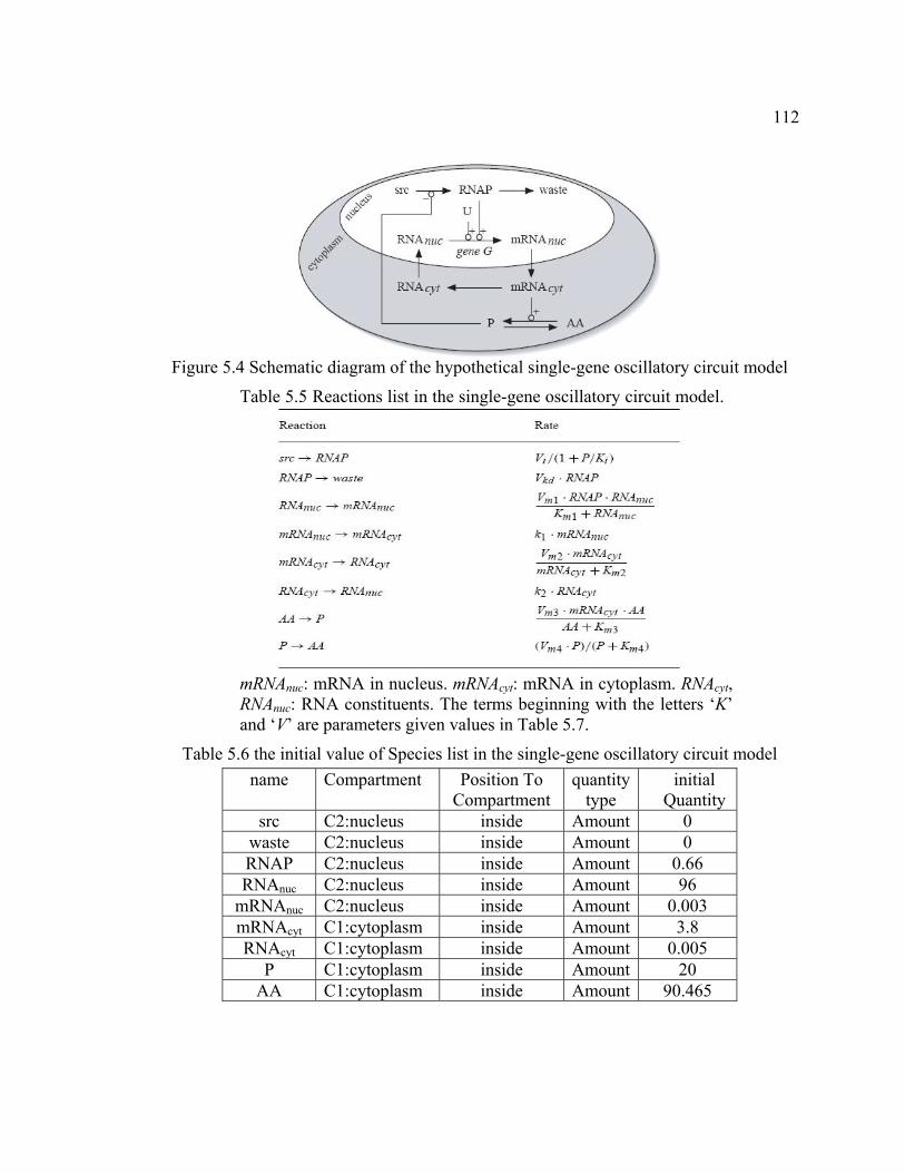
112
Figure 5.4 Schematic diagram of the hypothetical single-gene oscillatory circuit model
Table 5.5 Reactions list in the single-gene oscillatory circuit model.
mRNAnuc: mRNA in nucleus. mRNAcyt: mRNA in cytoplasm. RNAcyt, RNAnuc: RNA constituents. The terms beginning with the letters ‘K’ and ‘V’ are parameters given values in Table 5.7.
Table 5.6 the initial value of Species list in the single-gene oscillatory circuit model
name Compartment Position To Compartment
quantity type
initial Quantity
src C2:nucleus inside Amount 0 waste C2:nucleus inside Amount 0 RNAP C2:nucleus inside Amount 0.66 RNAnuc C2:nucleus inside Amount 96
mRNAnuc C2:nucleus inside Amount 0.003 mRNAcyt C1:cytoplasm inside Amount 3.8 RNAcyt C1:cytoplasm inside Amount 0.005
P C1:cytoplasm inside Amount 20 AA C1:cytoplasm inside Amount 90.465

113
Table 5.7 the parameters of the reactions in the single-gene oscillatory circuit model
name Vi Ki Vkd Vm1 Km1 Vm2 Km2 Vm3 Km3 Vm4 Km4 k1 k2 value 10 0.6 1 50 1 50 0.5 50 80 50 1 100 100
5.3.2 The simulation procedure of DEVS-SBML Platform
Base on the above of the hypothetical single-gene oscillatory circuit model’s
description and section 4.3 in last chapter, First step we can use the SBML specification
[56] to describe the model, in detail refer to Appendix A: singleGene.xml (SBML model
description file). Also we can use a structured diagram editor: CellDesignerTm [57] to
draw this model diagram to get the SBML model description file. Figure 5.5 is the
process diagram using software tool CellDesigner v3.5.2. The process diagram is a state
transition diagram that represents transition of the state of each molecule using arrows
that indicate transition and circle-headed arrows and bar-headed arrows to specify
promotion and inhibition of such transitions. We can use this tool to edit or change the
model, include initial value of the species, the parameters of reactions etc.
Figure 5.5 the process diagram of the single-gene oscillatory circuit model using software CellDesigner v3.5.2.

114
The following step we will translate SBML model into DEVSJAVA model, called
translator based on the development tool of SBML, libSBML [58]. LibSBML can read,
write, manipulate, and validate SBML files and data streams. So the translator reads all of
information of the single-gene oscillatory circuit model from the SBML file,
singGene.xml, to a string contained all of biological model information such as the
species, chemical reactions etc. And all chemically reacting information can be
represented by a means of kinetic rate equations or Michaelis-Menten and King-Altman
types of rate equations (see section 2.3.1). Then by the translator class, we construct
DEVS model files, package singleGene (refer to Appendix B). Then DEVSJAVA can
solve these differential equations by DEVS quantization integrator. The Figure 5.6 is the
viewer of DEVSJAVA ODE solver for the single-gene oscillatory circuit model.
Figure 5.6 the DEVS viewer for the single-gene oscillatory circuit model
To evaluate the performance of a DEVS simulation, we set up a DEVS ODE
model of the single-gene oscillatory circuit with the initial value of species in Table 5.6

115
and the parameters of the reactions in Table 5.7 respectively. We ran the single-gene
oscillatory circuit model for the first 20 seconds to trace the quantities of all species,
which is given in Figure 5.7.
Figure 5.7 Simulation results with Quantum Size (D) = 0.001 of all species for the single-gene oscillatory circuit model
5.3.3 Accuracy of DEVS-SBML simulation
The specie amino acids (AA) were selected to analyze the single-gene oscillatory
circuit model, because AA is biologically important, as it controls the expression level of
the proteins directly.
For the discussing the accuracy of DEVS-SBML Platform, we like to introduce
the result of CVODE as a benchmark. So the estimation and control of errors of CVODE
is very important. In CVODE, local truncation errors in the computed values of y are
estimated and the solver will control the vector e of estimated local errors in accordance

116
with a combination of input relative and absolute tolerances. Specifically the vector e is
made to satisfy an inequality of the form [87]
eWRMS, ewt ≤ 1 (5.4)
where the weighted root-mean-square norm eWRMS, w with weight vector w is defined
as
(5.5)
The CVODE error weight vector ewt has components
(5.6)
where the non-negative relative and absolute tolerances RTOL and ATOL are specified by
the user. Here RTOL is a scalar, but ATOL can be either a scalar or a vector.
The CVODE integrator computes an estimate ei of the local error at each time
step and strives to satisfy the inequality (5.4). eWRMS, w is the weighted root-mean-
square norm defined in terms of the user-defined relative and absolute tolerances (see
(5.5) and (5.6)). Since these tolerances define the allowed error per step, they should be
chosen conservatively. Experience indicates that a conservative choice yields a more
economical solution than error tolerances that are too large. The error control mechanism
in CVODE varies the step-size and order in an attempt to take minimum number of steps
while satisfying the local error test (5.4). Therefore it is important to pick all the tolerance
values conservatively, because they control the error committed on each individual time
N
wee
N
iii
wWRMS
1
2
,
)(
iii ATOLyRTOL
ewt
1

117
step. The final (global) errors are some sort of accumulation of those per-step errors. A
good rule of thumb is to reduce the tolerances by a factor of .01 from the actual desired
limits on errors. So if you want .01% accuracy (globally), a good choice is RTOL = 10-6.
But in any case, it is a good idea to do a few experiments with the tolerances to see how
the computed solution values vary as tolerances are reduced. In the following calculation
using CVODE solver, we setup RTOL = 10-6 and ATOL = 10-5, because the calculation
results of single-gene oscillatory circuit model using CVODE method are no big change
as RTOL is reduced from 10-6. So the final (global) errors of running single-gene model
using CVODE method are controlled to .01%.
The single-gene oscillatory circuit model was run using the DEVS (fine curve)
and CVODE (dot curve) methods, the simulation results for the first 10 time courses is
shown in Figure 5.8. We can see the trajectory of AA in the DEVS model almost matches
that of the CVODE method. No difference is by observing the simulation results between
the DEVS and CVODE in the first and second moments of the time course. An analysis
of higher moments showed a slight difference (Figure 5.8). However, as the overall
behavior of AA exemplifies, it can be seen that the simulation results of the DEVS and
the CVODE models agree well. It has been verified DEVS-SBML Platform is a right and
accurate software tool to the simulation of the biological process.

118
Figure 5.8 Simulation results of AA of the single-gene oscillatory circuit model for the DEVS model and the CVODE model. Comparison of AA time courses of the first 10 seconds of the simulation.
5.3.4 Error analysis in DEVS algorithm
Figure 5.9 (a) shows the simulation result with different values of Quantum Size
D. Even with large values of D, it can be seen that the simulation result remains bounded.
Figure 5.9 (b) shows the error in the simulation result for the more reasonable choices of
D. From the figure, the correspondence between a reduction in D and a reduction in the
computational error is readily apparent.

119
Figure 5.9 DEVS simulation results analysis of AA for the single-gene oscillatory circuit model (a) with different values of D. (b) absolute error of AA as a function of D.
Figure 5.10 demonstrates the execution time with Quantum Size D in DEVS
framework for the single-gene oscillatory circuit model. It can be seen that as the
quantum size D becomes bigger, the execution time becomes smaller. The execution time
reduction highly depends on the quantum size D. In Figure 5.9 (b) we already see that as
quantum size grows, the absolute error also grows. However, the model having bigger
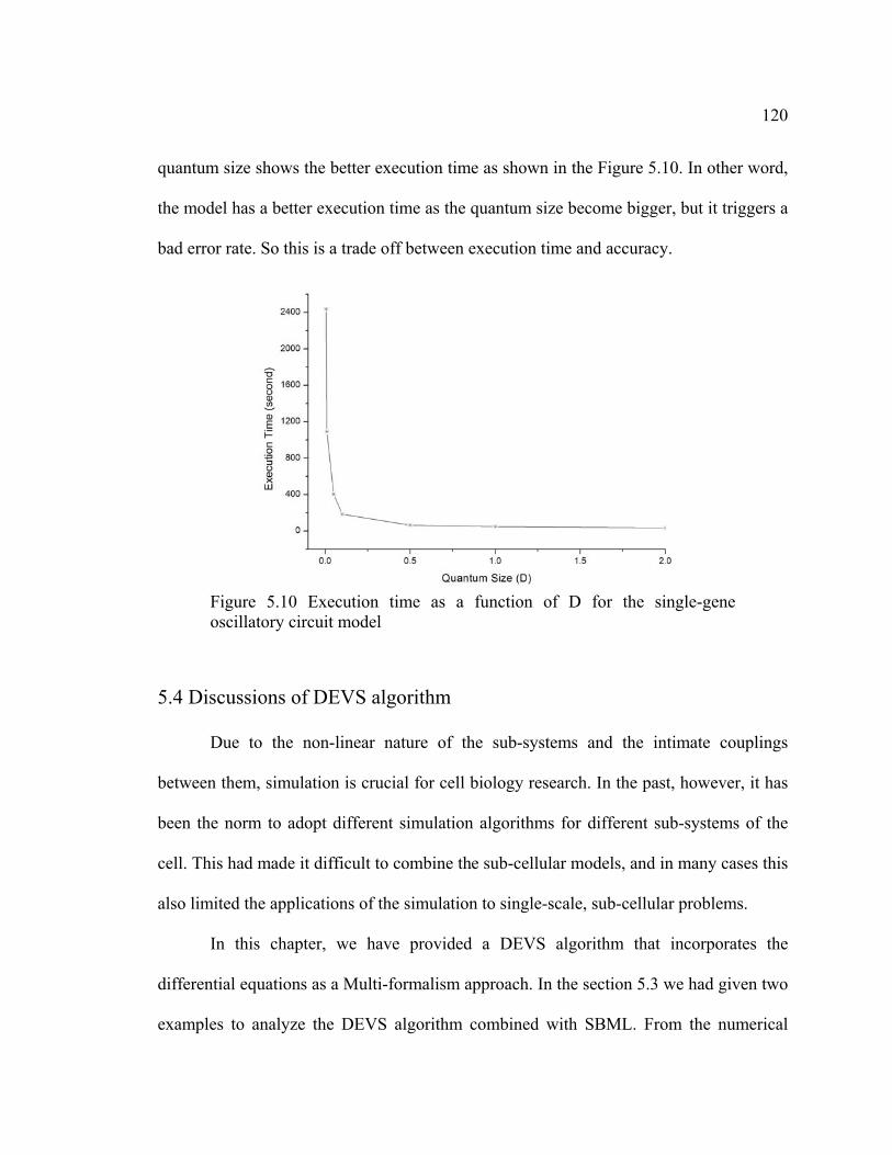
120
quantum size shows the better execution time as shown in the Figure 5.10. In other word,
the model has a better execution time as the quantum size become bigger, but it triggers a
bad error rate. So this is a trade off between execution time and accuracy.
Figure 5.10 Execution time as a function of D for the single-gene oscillatory circuit model
5.4 Discussions of DEVS algorithm
Due to the non-linear nature of the sub-systems and the intimate couplings
between them, simulation is crucial for cell biology research. In the past, however, it has
been the norm to adopt different simulation algorithms for different sub-systems of the
cell. This had made it difficult to combine the sub-cellular models, and in many cases this
also limited the applications of the simulation to single-scale, sub-cellular problems.
In this chapter, we have provided a DEVS algorithm that incorporates the
differential equations as a Multi-formalism approach. In the section 5.3 we had given two
examples to analyze the DEVS algorithm combined with SBML. From the numerical

121
experiments performed before, they were shown that this DEVS algorithm combined
with SBML can efficiently drive simulation models. We already analyzed the error and
execution time of DEVS combined with SBML which is shown that as quantum size D
grows, the absolute error also grows, but it triggers a bad execution time. The effects also
show that means of the DEVS ODE model and the stochastic Gillespie’s model agree
well. We also calculated the simulation result using the CVODE model and DEVS
model; it can be shown the results almost match.
The best algorithm for a specific model is determined by the nature of the target
system. Our DEVS algorithm combined with SBML provides a solution for situations in
which it is necessary to simulate processes concurrently across multiple scales of time,
space or concentration [84].

122
CHAPTER 6 CONCLUSIONS AND FUTURE WORKS
6.1 Conclusions
In a summary, this thesis discussed numerical simulations in more details in
computational cell biology in three parts.
First we overviewed the area of research, cell biology, from the viewpoint of
simulation studies, and commonly used modeling schemes and numerical methods have
been reviewed. We performed an analysis of some computational techniques in the
design of simulation algorithms and software platforms in this field of research.
Secondly, we reviewed the basic DEVS concept and DEVS formalism. We also
have inspected three basic system modeling formalisms: DEVS, DTSS and DESS. Multi-
algorithm framework, the combination of the DEVS and the DESS formalism, was
reviews in this thesis. The implementation of the integrator and Instantaneous Functions
to differential equations is given in DEVSJAVA Continuous package.
Lastly, a novel computational framework for cell biology simulation that can
drive different simulation models with DEVS combined with SBML, DEVS-SBML
Platform, has been introduced. This object-oriented framework based on DEVS defines
discrete and continuous ’transition functions’, and can incorporate virtually any discrete
and continuous simulation algorithms. By comparing the different deterministic
algorithms, Deterministic and Stochastic algorithm respectively, it is shown that DEVS-

123
SBML Platform can efficiently handle the biological models. Also one example is given
to show how to work using DEVS framework with SBML and how to translate SBML
model to DEVS model. Two relatively simple models, (1) the E. coli heat-shock response
model and (2) the single-gene oscillatory circuit model, are constructed. It was suggested
that this framework will likely be scaled up to more realistic, complex and large-scale
computational cell biology problems.
In a conclusion, we already have introduced new techniques to solve Biology
Processes using DEVS algorithm in this thesis. We can share biological models described
by DEVS-SBML Platform, which will be developed a new simulation platform. It was
shown that it enable biological simulations more efficient and faster using DEVS than
other methods, such as CVODE, the E-cell system etc. The performance measurement
shows how the quantum size of DEVS integrator affects execution time and error rate.
The numerical experimental result shows the followings clearly: the bigger quantum size
the biological models have, the higher error rate and the better execution time they have.
DEVS-SBML Platform, a generic software environment for computational cell biology,
is being under development. We also show the simulation procedure of DEVS-SBML
Platform, and how to work using the translator from SBML model to DEVS model. It has
been verified that, owing to its object-oriented design, DEVS-SBML Platform will be
implemented on a real software platform using Java language in an intuitive and efficient
way.
6.2 Future works

124
We achieve both evaluating the efficiency of the simulation results of biological
processes and performing the changes of the simulation results with Quantum Size D
over system cell biology. In addition, we also accomplish some comparisons DEVS ODE
models with stochastic models. However, there are further research works: developing
more realistic, complex and large-scale computational cell biology problems such as
metabolism, signal transduction pathways and gene expression systems etc., and further
investigating how to use the stochastic algorithm in the DEVS framework, due to the
stochastic models are generally believed to be more accurate to the real biological
processes. For the future work, it will be implemented the combination of the
deterministic and stochastic schemes into the DEVS framework to simulate the biological
models.
Another future work need to be continuously developed and implemented DEVS-
SBML Platform, a generic software environment. Design and implementation of a
generic computational framework and scientific software demand a way of thinking that
is completely different from ordinary virtues in many other scientific disciplines. Well
defined and concrete problems often characterize good problem-driven scientific projects,
whilst abstraction and generalization of the problems are the driving forces for the
algorithm and software developers. Although at the time of writing this it is somewhat
unclear that what extent of application domains are to be given to the algorithmic,
computational and software frameworks developed in this work successfully, we strongly
believe that, at least, necessity of the novel approach, DEVS combined with SBML, to
the computational problems those characterize the new field of computational cell

125
biology, including multi-formalism and multi-scale simulations, poses genuine challenges.
We hope that the ideas described in this thesis stimulate further discussions and
developments.

126
REFERENCES
[1] Zajicek, G., “A computer model simulating the behavior of adult red blood cells
in red cell model”, J. Theor. Biol. 19(1), 51–66, 1968
[2] King, E. L. and Altman, C., “A schematic method of deriving the rate laws for
enzyme-catalyzed reactions”, J. Phys. Chem. 60, 1375–1378, 1956
[3] Michaelis, L. and Menten, M. L., “Die kinetik der invertinwirkung”, Biochem. Z
49, 333–369, 1913
[4] Gear, C. W., “Numerical initial value problems in ordinary differential equations
Prentice-hall series in automatic computation”, Englewood Cliffs, N.J.: Prentice-
Hall, 1971
[5] Press, W. H., Teukolsky, S. A., Vetterling, W. T. and Flannery, B. P., “Numerical
recipes in C++: The art of scientific computing (2nd version)”, Cambridge; New
York: Cambridge University Press, 2002
[6] McAdams, H. H. and Shapiro, L., “Circuit simulation of genetic networks”,
Science 269(5224), 650–656, 1995
[7] Bray, D., Bourret, R. B. and Simon, M. I., “Computer simulation of the
phosphorylation cascade controlling bacterial chemotaxis”, Mol. Biol. Cell. 4(5),
469–482, 1993
127
[8] Morton-Firth, C. J. and Bray, D., “Predicting temporal fluctuations in an
intracellular signaling pathway”, J. Theor. Biol. 192(1), 117–128, 1998
[9] Morton-Firth, C. J., Shimizu, T. S. and Bray, D., “A free-energy-based stochastic
simulation of the tar receptor complex”, J. Mol. Biol. 286(4), 1059–1074, 1999
[10] Shimizu, T. S., Aksenov, S. V. and Bray, D., “A spatially extended stochastic
model of the bacterial chemotaxis signaling pathway”, J. Mol. Biol. 329(2), 291–
309, 2003
[11] Savageau, M. A., “Biochemical systems analysis: A study of function and design
in molecular biology”, Reading, Mass.: Addison-Wesley Pub. Co. Advanced
Book Program, 1976
[12] Hasty, J., McMillen, D., Isaacs, F. and Collins, J. J., “Computational studies of
gene regulatory networks: In numero molecular biology”, Nat. Rev. Genet. 2(4),
268-279, 2001
[13] Hashimoto, K., Miyoshi, F., Seno, A. and Tomita, M., “Generic gene expression
system for modeling complex gene regulation network using E-Cell system”, In
Genome Informatics, Tokyo, pp. 356–357. Universal Academy Press Inc, 1999
[14] Novitski, C. E. and Bajer, A. S., “Interaction of microtubules and the mechanism
of chromosome movement (zipper hypothesis). 3 theoretical analysis of energy
requirements and computer simulation of chromosome movement”, Cytobios
18(71-72), 173–182, 1978
[15] Gibbons, F., Chauwin, J. F., Desposito, M. and Jose, J. V., “A dynamical model
of kinesin-microtubule motility assays”, Biophys. J. 80(6), 2515–2526, 2001

128
[16] Tyson, J. J., Chen, K. and Novak, B., “Network dynamics and cell physiology”,
Nat. Rev. Mol. Cell. Biol. 2(12), 908–916, 2001
[17] Phair, R. D. and Misteli, T., “Kinetic modeling approaches to in vivo imaging”,
Nat. Rev. Mol. Cell. Biol. 2(12), 898–907, 2001
[18] Fehlberg, E., “Low-order classical runge-kutta formulas with step-size control and
their application to some heat transfer problems”, Technical Report NASA-TR-R-
315, NASA, 1969
[19] Hoffman J.D., “Numerical Methods for Engineers and Scientists”, (second
edition), Newton’s method, Page. 356, 2001
[20] Dormand, J. R. and Prince, P. J., “A family of embedded runge-kutta formulae”, J.
Comp. Appl. Math. 6, 19–26, 1980
[21] Hairer, E. and Wanner, G., “Solving Ordinary Differential Equations II: Stiff and
Differential-Algebraic Problems (2nd ed.)”, Volume 14 of Comput. Math. Berlin:
Springer, 1996
[22] Irvine, D. H. and Savageau, M. A., “Efficient solution of nonlinear ordinary
differential-equations expressed in s-system canonical form”, SIAM J. Num. Anal.
27(3), 704–735, 1990
[23] Gillespie, D. T. and Petzold, L. R., “Improved leap-size selection for accelerated
stochastic simulation”, J. Chem. Phys. 119(16), 8229, 2003
[24] McQuarrie, D. A., “Stochastic approach to chemical kinetics”, J. Appl. Prob. 4,
413–478, 1967

129
[25] Gillespie, D. T., “A rigorous derivation of the chemical master equation”, Physica
A 188, 404–425, 1992
[26] Gillespie, D. T., “A general method for numerically simulating the stochastic time
evolution of coupled chemical reactions”, J. Comp. Phys. 22, 403–434, 1976
[27] Gibson, M. A. and Bruck, J., “Efficient exact stochastic simulation of chemical
systems with many species and many channels”, J. Phys. Chem. A 104(9), 1876–
1889, 2000
[28] Matsumoto, M. and Nishimura, T., “Mersenne twister: A 623-dimensionally
equidistributed uniform pseudorandom number generator”, ACM Trans. Mod.
Comput. Sim. 8, 3–30, 1998
[29] Vasudeva, K. and Bhalla, U. S., “Adaptive stochastic-deterministic chemical
kinetic simulations”, Bioinformatics 20(1), 78–84, 2004
[30] Gillespie, D. T., “Approximate accelerated stochastic simulation of chemically
reacting systems”, J. Chem. Phys. 115(4), 1716–1733, 2001
[31] Bochner, Salomon, "John von Neumann", Biographical Memoirs, Vol. 32,
National Academy of Sciences, pp. 456-451, 1958
[32] Dawson, S. P., Chen, S. and Doolen, G. D., “Lattice boltzmann computations for
reaction-diffusion equations”, J. Chem. Phys. 98(2), 1514–1523, 1993
[33] Weimar, J. R., “Cellular automata approaches to enzymatic reaction networks”, In
S. Bandini, B. Chopard, and M. Tomassini (Eds.), 5th International Conference
on Cellular Automata for Research and Industry ACRI, Lecture Notes in
Computer Science, Switzerland, pp. 294–303. Springer, 2002

130
[34] Patel, A. A., Gawlinski, E. T., Lemieux, S. K. and Gatenby, R. A., “A cellular
automaton model of early tumor growth and invasion”, J. Theor. Biol. 213(3),
315–331, 2001
[35] Ermentrout, G. B. and Edelstein-Keshet, L., “Cellular automata approaches to
Biological modeling”, J. Theor. Biol. 160(1), 97–133, 1993
[36] Yugi, K., Nakayama, Y. and Tomita, M., “A hybrid static/dynamic simulation
algorithm: Towards large-scale pathway simulation”, In E. Aurell, J. Elf, and J.
Jeppsson (Eds.), the 3rd. International Conference on Systems Biology, pp. 235,
2002
[37] Bartol, T. M. J., Stiles, J. R., Salpeter, M. M., Salpeter, E. E. and Sejnowski, T. J.,
“Mcell: generalized monte-carlo computer simulation of synaptic transmission
and chemical signaling”, Soc. Neurosci. Abstr. 22, 1742, 1996
[38] Barshop, B. A. Wrenn, R. F. and Frieden, C., “Analysis of numerical methods for
computer simulation of kinetic processes: Development of kinsim–a flexible,
portable system”, Anal. Biochem. 130(1), 134–145, 1983
[39] Mendes, P., “Gepasi: A software package for modeling the dynamics, steady
states and control of biochemical and other systems”, Comput. Appl. Biosci. 9(5),
563–571, 1993
[40] Goryanin, I., Hodgman, T. C. and Selkov, E., “Mathematical simulation and
analysis of cellular metabolism and regulation”, Bioinformatics 15(9), 749–758,
1999
131
[41] Ginkel, M., Kremling, A., Nutsch, T., Rehner, R. and Gilles, E. D., “Modular
modeling of cellular systems with ProMoT/Diva”, Bioinformatics 19(9), 1169–76,
2003
[42] Kootsey, J. M., Kohn, M. C., Feezor, M. D., Mitchell, G. R. and Fletcher, P. R.,
“Scop: An interactive simulation control program for micro- and minicomputers”,
Bull. Math. Biol. 48(3-4), 427–441, 1986
[43] Ichikawa, K., “A-cell: Graphical user interface for the construction of
biochemical reaction models”, Bioinformatics 17(5), 483–484, 2001
[44] McAdams, H. H. and Arkin, A., “Simulation of prokaryotic genetic circuits”,
Annu. Rev. Biophys. Biomol. Struct. 27, 199–224, 1998
[45] Sauro, H. M., “Scamp: A general-purpose simulator and metabolic control
analysis program”, Comput. Appl. Biosci. 9(4), 441–450, 1993
[46] Loew, L. M. and Schaff, J. C., “The virtual cell: A software environment for
computational cell biology”, Trends Biotechnol. 19(10), 401–406, 2001
[47] Ferreira A, “PLAS: Power Law Analysis and Simulation”, 2005
http://www.dqb.fc.ul.pt/docentes/aferreira/plas.html
[48] Le Novere, N. and Shimizu, T. S., “StochSim: Modeling of stochastic bimolecular
processes”, Bioinformatics 17(6), 575–576, 2001
[49] Hucka, M., Finney, A., Sauro, H. M., Bolouri, H., Doyle, J. C., Kitano, H. Arkin,
A. P., Bornstein, B. J., Bray, D., Cornish-Bowden, A., Cuellar, A. A., Dronov, S.,
Gilles, E. D., Ginkel, M., Gor, V., Goryanin, I. I., Hedley, W. J., Hodgman, T. C.,
Hofmeyr, J., Hunter, P. J., Juty, N. S., Kasberger, J. L., Kremling, A., Kummer,

132
U., Le Novere, N., Loew, L. M., Lucio, D., Mendes, P., Minch, E., Mjolsness, E.
D., Nakayama, Y., Nelson, M. R., Nielsen, P. F., Sakurada, T., Schaff, J. C.,
Shapiro, B. E., Shimizu, T. S., Spence, H. D., Stelling, J., Takahashi, K., Tomita,
M., Wagner, J. and Wang, J., “The systems biology markup language (sbml): a
medium for representation and exchange of biochemical network models”,
Bioinformatics 19(4), 524–531, 2003
[50] Hedley, W. J., Nelson, M. R., Bullivant, D. P. and Nielson, P. F., “A short
introduction to CellML”, Phil. Trans. Roy. Soc. London A, 359, 1073–1089, 2001
[51] Hucka, M., Finney, A., Sauro, H. M., Bolouri, H., Doyle, J. and Kitano, H., “The
Erato systems biology workbench: Enabling interaction and exchange between
software tools for computational biology”, In Pacific Symposium on Bio-
computing, Volume 7, pp. 450–461, 2002
[52] Kitano, H., “Systems biology: a brief overview”, Science, 295, 1662–1664, 2002
[53] Abbott, A., “Alliance of US labs plans to build map of cell signaling pathways”,
Nature, 402, 219–220, 1999
[54] Bray, T., Paoli, J. and Sperberg-McQueen, C. M., “Extensible markup language
(XML) 1.0”, http://www.w3.org/TR/1998/REC-xml-19980210, 1998
[55] Achard, F., Vaysseix, G. and Barillot, E., “XML, bioinformatics and data
integration”, Bioinformatics, 17, 115–125.
[56] SBML Level Document: http://www.sbml.org/documents/
[57] Celldesigner: http://www. celldesigner.org/
[58] LibSBML: http://www.sbml.org/downloads/

133
[59] Bernard P. Zeigler, Hessam S. Sarjoughian, “DEVS Component-Based M&S
Framework: An Introduction”, AIS 2002
[60] X. Hu, “A Simulation-based Software Development Methodology for Distributed
Real-time Systems”, Ph. D. Dissertation, Fall 2003, Electrical and Computer
Engineering Dept., University of Arizona
[61] Bernard P. Zeigler, Tag Gon Kim and Herbert Praehofer, “Theory of Modeling
and Simulation”, Academic Press, 2000
[62] William H. Press, Saul A. Teukolsky, William T. Vetterling, Brian P. Flannery,
“Numerical Recipes in C”, Second Edition. Cambridge University Press, 1992
[63] Richard L. Burden, J. Douglas Faires, “Numerical Analysis”, Fourth Edition,
PWS-KENT Publishing Company, 1989
[64] B.P. Zeigler and Hessam S. Sarjoughian, “Introduction to DEVS Modeling &
Simulation with JAVA”, ACIMS publication, Arizona Center for Integrative
Modeling and Simulation, Tucson, Arizona
http://www.acims.arizona.edu/SOFTWARE/devsjava_licensed/CBMSManuscript
.zip
[65] E. Kofman, M. Lapadula, and E. Pagliero, “Powerdevs: A devs-based
environment for hybrid system modeling and simulation”, Technical Report
LSD0306, School of Electronic Engineering, Universidad Nacional de Rosario,
Rosario, Argentina, 2003

134
[66] A. Muzy and J. Nutaro, “Algorithms for efficient implementations of the devs &
dsdevs abstract simulators”, In 1st Open International Conference on Modeling &
Simulation, pages 401-407, ISIMA/Blaise Pascal University, France, June 2005
[67] Bernard P. Zeigler and Hessam S. Sarjoughian, “Introduction to devs modeling
and simulation with java: Developing component-based simulation models”,
Unpublished manuscript, 2005
[68] Gabriel Wainer, “Cd++: a toolkit to develop devs models”, Software: Practice
and Experience, 32(13):1261-1306, 2002
[69] Jean-Baptiste Filippi and Paul Bisgambiglia, “Jdevs: an implementation of a devs
based formal framework for environmental modeling”, Environmental Modeling
& Software, 19(3):261-274, March 2004
[70] DEVSJAVA Continuous package: http://www.acims.arizona.edu
[71] Takahashi, K., Yugi, K., Hashimoto, K., Yamada, Y., Pickett, C. J. F. and Tomita,
M., “Computational challenges in cell simulation: A software engineering
approach”, IEEE Intell. Syst., 17(5), 64–71, 2002
[72] http://www.u.arizona.edu/~saurabh/devsml/devsml.html
[73] Badros, G., “JavaML: a Markup Language for Java Source Code”, Proceedings of
the 9th International World Wide Web Conference on Computer Networks: the
international journal of computer and telecommunication networking, pages 159-
177

135
[74] Gross, C. A., “Function and regulation of the heat shock proteins”, In F. C.
Neidhardt and R. Curtiss (Eds.), Escherichia coli and Salmonella: Cellular and
molecular biology (2nd ed.), pp. 1382–1399. Washington, D.C.: ASM Press, 1996
[75] Grossman, A. D., Straus, D. B., Walter, W. A. and Gross, C. A., “Sigma 32
synthesis can regulate the synthesis of heat shock proteins in Escherichia coli.
Genes Dev”, 1(2), 179–184, 1987
[76] Gamer, J., Multhaup, G., Tomoyasu, T., McCarty, J. S., Rudiger, S., Schonfeld, H.
J., Schirra, C., Bujard, H. and Bukau, B., “A cycle of binding and release of the
dnak, dnaj and grpe chaperones regulates activity of the Escherichia coli heat
shock transcription factor sigma32”, EMBO J. 15(3), 607–617
[77] Srivastava, R., Peterson, M. S. and Bentley, W. E., “Stochastic kinetic analysis of
the Escherichia coli stress circuit using sigma (32)-targeted antisense”, Biotechnol.
Bioeng, 75(1), 120–129.
[78] Kouichi Takahashi, Kazunari Kaizu, Bin Hu, and Masaru Tomita, “A Multi-
algorithm, Multi-timescale Method for Cell Simulation”, Bioinformatics, 20: 538-
546, 2004
[79] S. D. Cohen and A. C. Hindmarsh, “CVODE, A Stiff/Non-stiff ODE Solver in C”,
Computers in Physics, 10(2), pp. 138-143, 1996
https://computation.llnl.gov/casc/sundials/documentation/documentation.html
[80] R. Jammalamadaka, “Activity characterization of spatial models: Application to
the discrete event solution of partial differential equations”, Master's thesis,
University of Arizona, Tucson, Arizona, USA, 2003

136
[81] Alexandre Muzy, Paul-Antoine Santoni, Bernard P. Zeigler, James J. Nutaro, and
Rajanikanth Jammalamadaka, “Discrete event simulation of large-scale spatial
continuous systems”, In Simulation Multi-conference, 2005
[82] Gillespie, D. T., “Concerning the validity of the stochastic approach of chemical
kinetics”, J. Stat. Phys. 16, 311–319, 1977
[83] Singer, K., “Application of the theory of stochastic processes to the study of
irreproducible chemical reactions and nucleation processes”, J. R. Stat. Soc. B 15,
92–106, 1953
[84] Rao, C. V., Wolf, D. M. and Arkin, A. P., “Control, exploitation and tolerance of
intracellular noise”, Nature 420(6912), 231–237, 2002
[85] Marion, G., Renshaw, E. and Gibson, G., “Stochastic effects in a model of
nematode infection in ruminants”, IMA J. Math. Appl. Med. Biol. 15(2), 97–116,
1998
[86] Srivastava, R., You, L., Summers, J. and Yin, J., “Stochastic vs. deterministic
modeling of intracellular viral kinetics”, J. Theor. Biol. 218(3), 309–321, 2002
[87] User Documentation for CVODE v2.6.0
https://computation.llnl.gov/casc/sundials/documentation/cv_guide.pdf
Example Programs for CVODE v2.6.0
https://computation.llnl.gov/casc/sundials/documentation/cv_examples.pdf

137
APPENDIX A: SingleGene.xml
<?xml version="1.0" encoding="UTF-8"?> <sbml xmlns="http://www.sbml.org/sbml/level2" level="2" version="1"> <model id="Single_Gene"> <listOfCompartments> <compartment id="default" size="1"/> <compartment id="c1" name="Cytoplasm" size="1" outside="default"/> <compartment id="c2" name="nucleus" size="1" outside="c1"/> </listOfCompartments> <listOfSpecies> <species id="s1" name="src" compartment="c2" initialAmount="0" boundaryCondition="true" charge="0"/> <species id="s2" name="waste" compartment="c2" initialAmount="0" boundaryCondition="true" charge="0"/> <species id="s3" name="RNAP" compartment="c2" initialAmount="0.66" charge="0"/> <species id="s4" name="RNAnuc" compartment="c2" initialAmount="96" charge="0"/> <species id="s5" name="mRNAnuc" compartment="c2" initialAmount="0.003" charge="0"/> <species id="s6" name="mRNAcyt" compartment="c1" initialAmount="3.8" charge="0"/> <species id="s7" name="RNAcyt" compartment="c1" initialAmount="0.005" charge="0"/> <species id="s8" name="P" compartment="c1" initialAmount="20" charge="0"/> <species id="s9" name="AA" compartment="c1" initialAmount="90.465" charge="0"/> </listOfSpecies> <listOfReactions> <reaction id="re1" reversible="false" fast="false"> <listOfReactants> <speciesReference species="s1"/> </listOfReactants> <listOfProducts> <speciesReference species="s3"/> </listOfProducts> <listOfModifiers> <modifierSpeciesReference species="s8"/> </listOfModifiers> <kineticLaw> <math xmlns="http://www.w3.org/1998/Math/MathML"> <apply>

138
<divide/> <ci> Vi </ci> <apply> <plus/> <cn type="integer"> 1 </cn> <apply> <divide/> <ci> s8 </ci> <ci> Ki </ci> </apply> </apply> </apply> </math> <listOfParameters> <parameter id="Vi" value="10"/> <parameter id="Ki" value="0.6"/> </listOfParameters> </kineticLaw> </reaction> <reaction id="re2" reversible="false" fast="false"> <listOfReactants> <speciesReference species="s3"/> </listOfReactants> <listOfProducts> <speciesReference species="s2"/> </listOfProducts> <kineticLaw> <math xmlns="http://www.w3.org/1998/Math/MathML"> <apply> <times/> <ci> Vkd </ci> <ci> s3 </ci> </apply> </math> <listOfParameters> <parameter id="Vkd" value="1"/> </listOfParameters> </kineticLaw> </reaction> <reaction id="re3" reversible="false" fast="false"> <listOfReactants> <speciesReference species="s4"/>

139
</listOfReactants> <listOfProducts> <speciesReference species="s5"/> </listOfProducts> <listOfModifiers> <modifierSpeciesReference species="s3"/> </listOfModifiers> <kineticLaw> <math xmlns="http://www.w3.org/1998/Math/MathML"> <apply> <divide/> <apply> <times/> <ci> Vm1 </ci> <ci> s3 </ci> <ci> s4 </ci> </apply> <apply> <plus/> <ci> s4 </ci> <ci> Km1 </ci> </apply> </apply> </math> <listOfParameters> <parameter id="Vm1" value="50"/> <parameter id="Km1" value="1"/> </listOfParameters> </kineticLaw> </reaction> <reaction id="re6" reversible="false" fast="false"> <listOfReactants> <speciesReference species="s6"/> </listOfReactants> <listOfProducts> <speciesReference species="s7"/> </listOfProducts> <kineticLaw> <math xmlns="http://www.w3.org/1998/Math/MathML"> <apply> <divide/> <apply> <times/>

140
<ci> Vm2 </ci> <ci> s6 </ci> </apply> <apply> <plus/> <ci> s6 </ci> <ci> Km2 </ci> </apply> </apply> </math> <listOfParameters> <parameter id="Vm2" value="50"/> <parameter id="Km2" value="0.5"/> </listOfParameters> </kineticLaw> </reaction> <reaction id="re7" reversible="false" fast="false"> <listOfReactants> <speciesReference species="s9"/> </listOfReactants> <listOfProducts> <speciesReference species="s8"/> </listOfProducts> <listOfModifiers> <modifierSpeciesReference species="s6"/> </listOfModifiers> <kineticLaw> <math xmlns="http://www.w3.org/1998/Math/MathML"> <apply> <divide/> <apply> <times/> <ci> Vm3 </ci> <ci> s6 </ci> <ci> s9 </ci> </apply> <apply> <plus/> <ci> s9 </ci> <ci> Km3 </ci> </apply> </apply> </math>

141
<listOfParameters> <parameter id="Vm3" value="50"/> <parameter id="Km3" value="80"/> </listOfParameters> </kineticLaw> </reaction> <reaction id="re8" reversible="false" fast="false"> <listOfReactants> <speciesReference species="s8"/> </listOfReactants> <listOfProducts> <speciesReference species="s9"/> </listOfProducts> <kineticLaw> <math xmlns="http://www.w3.org/1998/Math/MathML"> <apply> <divide/> <apply> <times/> <ci> Vm4 </ci> <ci> s8 </ci> </apply> <apply> <plus/> <ci> s8 </ci> <ci> Km4 </ci> </apply> </apply> </math> <listOfParameters> <parameter id="Vm4" value="50"/> <parameter id="Km4" value="1"/> </listOfParameters> </kineticLaw> </reaction> <reaction id="re9" reversible="false" fast="false"> <listOfReactants> <speciesReference species="s5"/> </listOfReactants> <listOfProducts> <speciesReference species="s6"/> </listOfProducts>
142
<kineticLaw> <math xmlns="http://www.w3.org/1998/Math/MathML"> <apply> <times/> <ci> k1 </ci> <ci> s5 </ci> </apply> </math> <listOfParameters> <parameter id="k1" value="100"/> </listOfParameters> </kineticLaw> </reaction> <reaction id="re10" reversible="false" fast="false"> <listOfReactants> <speciesReference species="s7"/> </listOfReactants> <listOfProducts> <speciesReference species="s4"/> </listOfProducts> <kineticLaw> <math xmlns="http://www.w3.org/1998/Math/MathML"> <apply> <times/> <ci> k2 </ci> <ci> s7 </ci> </apply> </math> <listOfParameters> <parameter id="k2" value="100"/> </listOfParameters> </kineticLaw> </reaction> </listOfReactions> </model> </sbml>

143
APPENDIX B: Package singleGene using DEVS model
Package singleGene describe the hypothetical single-gene oscillatory circuit
model in DEVS framework using Java language. Package singleGene is generated
automatically by the translator from the SBML model to the DEVS model. Package
singleGene include several Java source code files:
singleGene.java: display chemical reactions of the single-gene model using DEVS
Integrators
x_AARate.java: the kinetic Law rate of the specie AA
x_mRNAcytRate.java: the kinetic Law rate of the specie mRNAcyt
x_mRNAnucRate.java: the kinetic Law rate of the specie mRNAnuc
x_PRate.java: the kinetic Law rate of the specie P
x_RNAcytRate.java: the kinetic Law rate of the specie RNAcyt
x_RNAnucRate.java: the kinetic Law rate of the specie RNAnuc
x_RNAPRate.java: the kinetic Law rate of the specie RNAP
x_srcRate.java: the kinetic Law rate of the specie src
x_wasteRate.java: the kinetic Law rate of the specie waste