cellular network analysis - University of Wisconsin–Madison

Comparative Network Analysis

BMI/CS 776www.biostat.wisc.edu/bmi776/

Spring 2012Colin Dewey

[email protected]

Protein-protein Interaction Networks

104 | FEBRUARY 2004 | VOLUME 5 www.nature.com/reviews/genetics

R E V I EW S

mathematical properties of random networks14. Theirmuch-investigated random network model assumes thata fixed number of nodes are connected randomly to eachother (BOX 2). The most remarkable property of the modelis its ‘democratic’or uniform character, characterizing thedegree, or connectivity (k ; BOX 1), of the individual nodes.Because, in the model, the links are placed randomlyamong the nodes, it is expected that some nodes collectonly a few links whereas others collect many more. In arandom network, the nodes degrees follow a Poissondistribution, which indicates that most nodes haveroughly the same number of links, approximately equalto the network’s average degree, <k> (where <> denotesthe average); nodes that have significantly more or lesslinks than <k> are absent or very rare (BOX 2).

Despite its elegance, a series of recent findings indi-cate that the random network model cannot explainthe topological properties of real networks. The deviations from the random model have several keysignatures, the most striking being the finding that, incontrast to the Poisson degree distribution, for manysocial and technological networks the number of nodeswith a given degree follows a power law. That is, theprobability that a chosen node has exactly k links follows P(k) ~ k –γ, where γ is the degree exponent, withits value for most networks being between 2 and 3 (REF. 15). Networks that are characterized by a power-lawdegree distribution are highly non-uniform, most ofthe nodes have only a few links. A few nodes with a verylarge number of links, which are often called hubs, holdthese nodes together. Networks with a power degreedistribution are called scale-free15, a name that is rootedin statistical physics literature. It indicates the absenceof a typical node in the network (one that could beused to characterize the rest of the nodes). This is instrong contrast to random networks, for which thedegree of all nodes is in the vicinity of the averagedegree, which could be considered typical. However,scale-free networks could easily be called scale-rich aswell, as their main feature is the coexistence of nodes ofwidely different degrees (scales), from nodes with oneor two links to major hubs.

Cellular networks are scale-free. An important develop-ment in our understanding of the cellular networkarchitecture was the finding that most networks withinthe cell approximate a scale-free topology. The first evi-dence came from the analysis of metabolism, in whichthe nodes are metabolites and the links representenzyme-catalysed biochemical reactions (FIG. 1).As manyof the reactions are irreversible, metabolic networks aredirected. So, for each metabolite an ‘in’ and an ‘out’degree (BOX 1) can be assigned that denotes the numberof reactions that produce or consume it, respectively.The analysis of the metabolic networks of 43 differentorganisms from all three domains of life (eukaryotes,bacteria, and archaea) indicates that the cellular metabo-lism has a scale-free topology, in which most metabolicsubstrates participate in only one or two reactions, but afew, such as pyruvate or coenzyme A, participate indozens and function as metabolic hubs16,17.

Depending on the nature of the interactions, net-works can be directed or undirected. In directednetworks, the interaction between any two nodes has awell-defined direction, which represents, for example,the direction of material flow from a substrate to aproduct in a metabolic reaction, or the direction ofinformation flow from a transcription factor to the genethat it regulates. In undirected networks, the links donot have an assigned direction. For example, in proteininteraction networks (FIG. 2) a link represents a mutualbinding relationship: if protein A binds to protein B,then protein B also binds to protein A.

Architectural features of cellular networksFrom random to scale-free networks. Probably the mostimportant discovery of network theory was the realiza-tion that despite the remarkable diversity of networksin nature, their architecture is governed by a few simpleprinciples that are common to most networks of majorscientific and technological interest9,10. For decadesgraph theory — the field of mathematics that dealswith the mathematical foundations of networks —modelled complex networks either as regular objects,such as a square or a diamond lattice, or as completelyrandom network13. This approach was rooted in theinfluential work of two mathematicians, Paul Erdös,and Alfréd Rényi, who in 1960 initiated the study of the

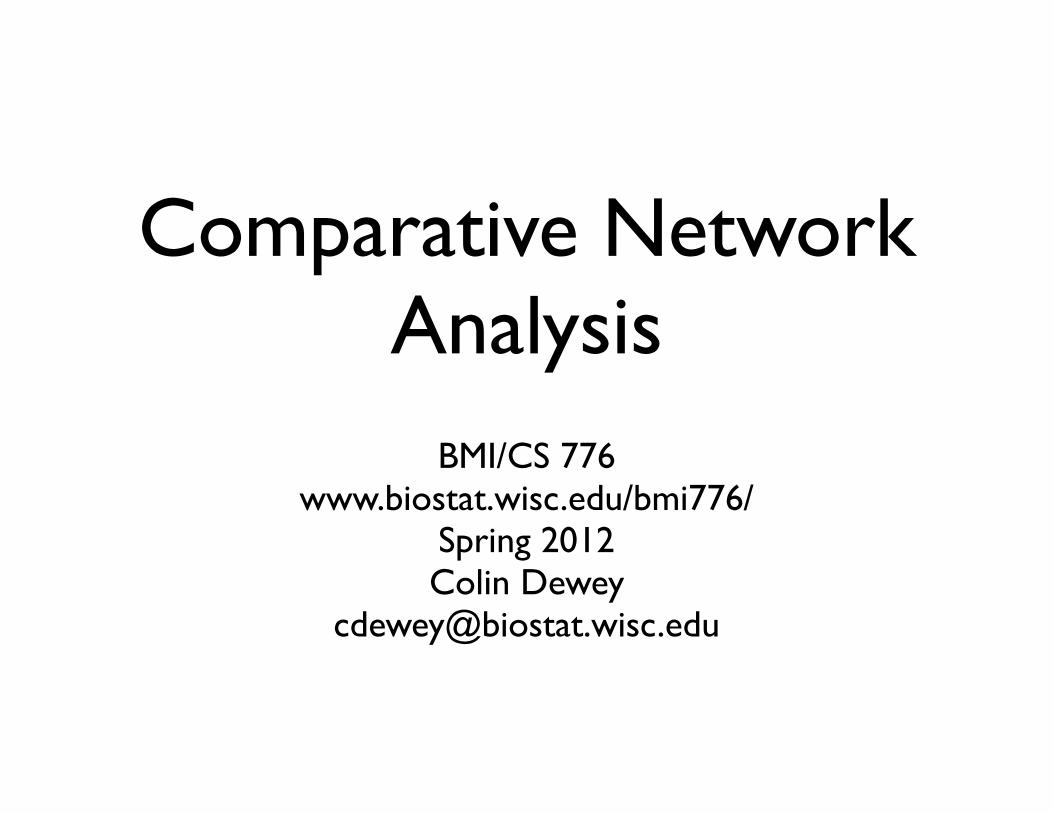
Figure 2 | Yeast protein interaction network. A map of protein–protein interactions18 inSaccharomyces cerevisiae, which is based on early yeast two-hybrid measurements23, illustratesthat a few highly connected nodes (which are also known as hubs) hold the network together.The largest cluster, which contains ~78% of all proteins, is shown. The colour of a node indicatesthe phenotypic effect of removing the corresponding protein (red = lethal, green = non-lethal,orange = slow growth, yellow = unknown). Reproduced with permission from REF. 18 ©Macmillan Magazines Ltd.

• Yeast protein interactions from yeast two-hybrid experiments

• Largest cluster in network contains 78% of proteins

lethalnon-lethalslow growthunknown

Knock-out phenotype

(Jeong et al., 2001, Nature)

Overview

• Experimental techniques for determining networks

• Properties of biological networks

• Comparative network tasks

Experimental techniques

• Yeast two-hybrid system

• Protein-protein interactions

• Microarrays

• Expression patterns of mRNAs

• Similar patterns imply involvement in same regulatory or signaling network

• Knock-out studies

• Identify genes required for synthesis of certain molecules

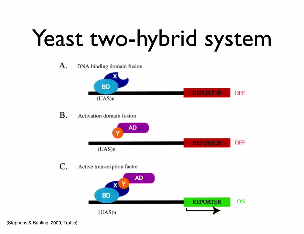
Yeast two-hybrid system

(Stephens & Banting, 2000, Traffic)

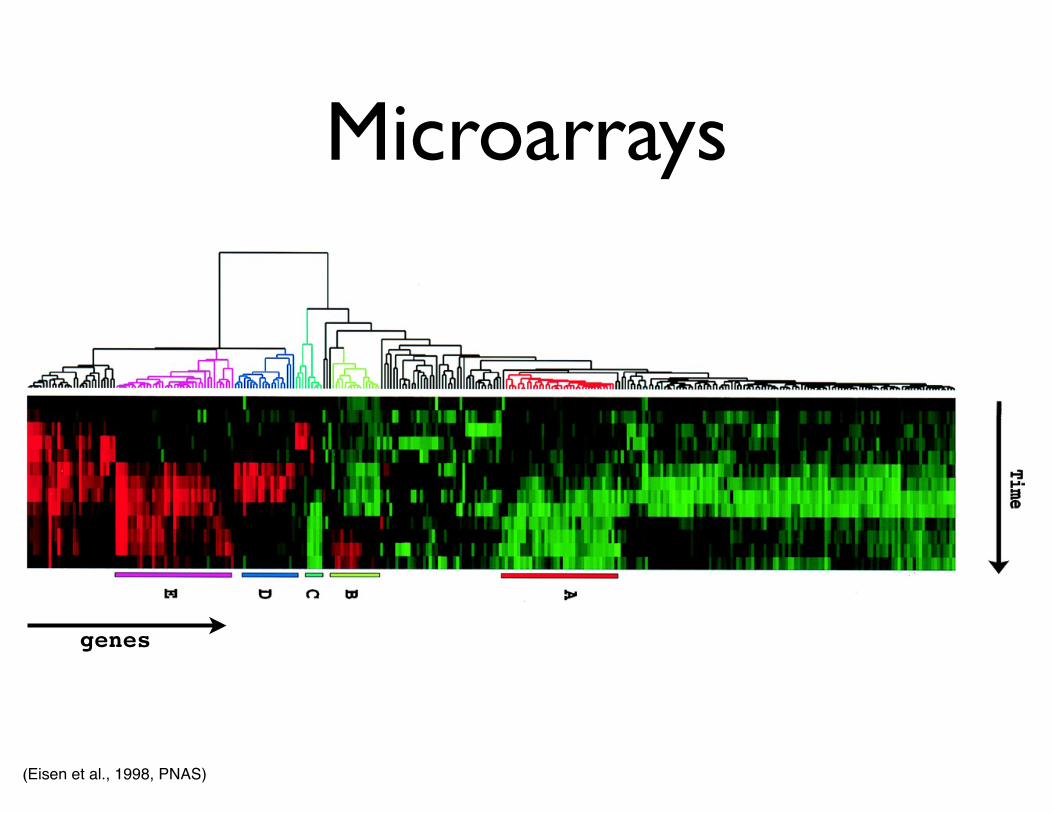
Microarrays

(Eisen et al., 1998, PNAS)

genes

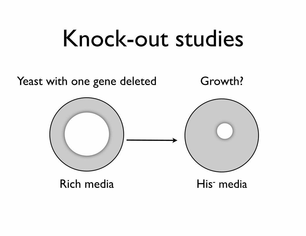
Knock-out studies

Rich media His- media

Growth?Yeast with one gene deleted

Topological properties of networks

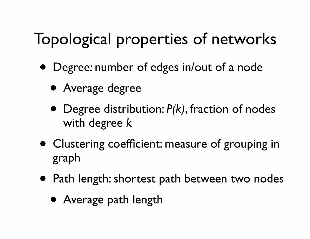
• Degree: number of edges in/out of a node

• Average degree

• Degree distribution: P(k), fraction of nodes with degree k

• Clustering coefficient: measure of grouping in graph

• Path length: shortest path between two nodes

• Average path length

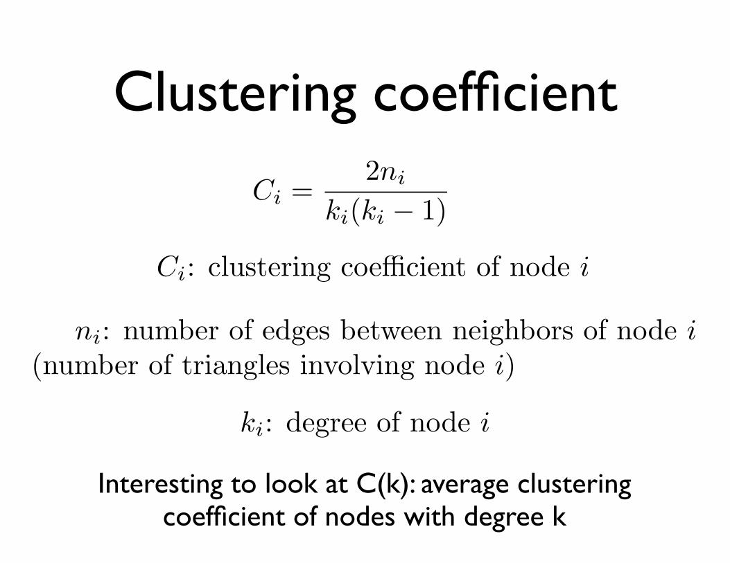
Clustering coefficient

Ci: clustering coe�cient of node i

ni: number of edges between neighbors of node i(number of triangles involving node i)

Ci =2ni

ki(ki � 1)

ki: degree of node i

Interesting to look at C(k): average clustering coefficient of nodes with degree k

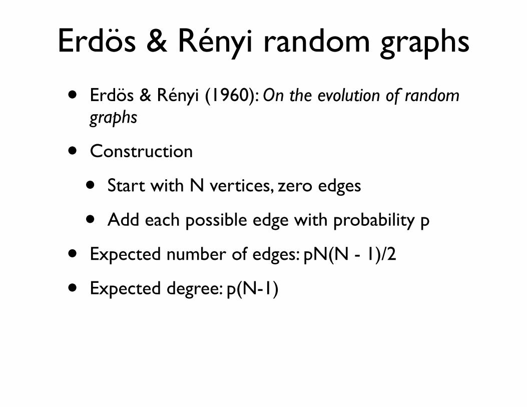
Erdös & Rényi random graphs

• Erdös & Rényi (1960): On the evolution of random graphs

• Construction

• Start with N vertices, zero edges

• Add each possible edge with probability p

• Expected number of edges: pN(N - 1)/2

• Expected degree: p(N-1)

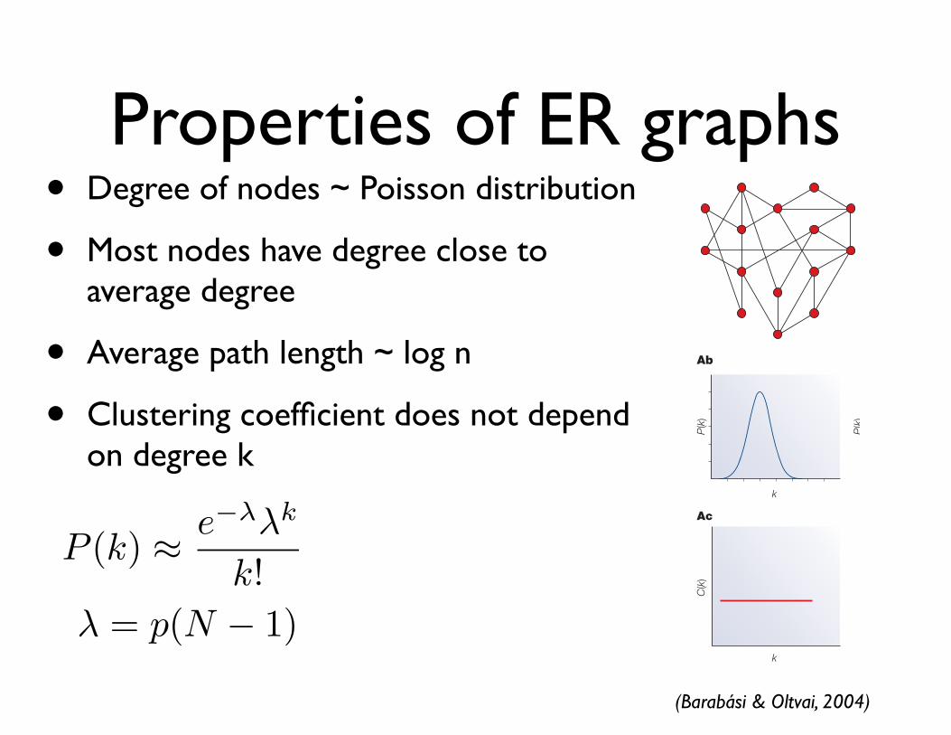
Properties of ER graphs• Degree of nodes ~ Poisson distribution

• Most nodes have degree close to average degree

• Average path length ~ log n

• Clustering coefficient does not depend on degree k

NATURE REVIEWS | GENETICS VOLUME 5 | FEBRUARY 2004 | 105

R E V I EW S

Box 2 | Network models

Network models are crucial for shaping our understanding of complex networks and help to explain the origin of observed networkcharacteristics. There are three models that had a direct impact on our understanding of biological networks.

Random networks The Erdös–Rényi (ER) model of a random network14 (see figure, part A) starts with N nodes and connects each pair of nodes with probability p,which creates a graph with approximately pN(N–1)/2 randomly placed links (see figure, part Aa). The node degrees follow a Poisson distribution(see figure, part Ab), which indicates that most nodes have approximately the same number of links (close to the average degree <k>). The tail(high k region) of the degree distribution P(k) decreases exponentially, which indicates that nodes that significantly deviate from the average areextremely rare. The clustering coefficient is independent of a node’s degree, so C(k) appears as a horizontal line if plotted as a function of k (seefigure, part Ac). The mean path length is proportional to the logarithm of the network size, l ~ log N, which indicates that it is characterized by thesmall-world property.

Scale-free networksScale-free networks (see figure, part B) are characterized by a power-law degree distribution; the probability that a node has k links follows P(k) ~ k –γ, where γ is the degree exponent. The probability that a node is highly connected is statistically more significant than in a random graph,the network’s properties often being determined by a relatively small number of highly connected nodes that are known as hubs (see figure, partBa; blue nodes). In the Barabási–Albert model of a scale-free network15, at each time point a node with M links is added to the network, whichconnects to an already existing node I with probability ΠI = kI/ΣJkJ, where kI is the degree of node I (FIG. 3) and J is the index denoting the sum overnetwork nodes. The network that is generated by this growth process has a power-law degree distribution that is characterized by the degreeexponent γ = 3. Such distributions are seen as a straight line on a log–log plot (see figure, part Bb). The network that is created by theBarabási–Albert model does not have an inherent modularity, so C(k) is independent of k (see figure, part Bc). Scale-free networks with degreeexponents 2<γ<3, a range that is observed in most biological and non-biological networks, are ultra-small34,35, with the average path lengthfollowing ! ~ log log N, which is significantly shorter than log N that characterizes random small-world networks.

Hierarchical networksTo account for the coexistence of modularity, local clustering and scale-free topology in many real systems it has to be assumed that clusterscombine in an iterative manner, generating a hierarchical network47,53 (see figure, part C). The starting point of this construction is a small clusterof four densely linked nodes (see the four central nodes in figure, part Ca). Next, three replicas of this module are generated and the three externalnodes of the replicated clustersconnected to the central node ofthe old cluster, which produces alarge 16-node module. Threereplicas of this 16-node moduleare then generated and the 16peripheral nodes connected tothe central node of the oldmodule, which produces a newmodule of 64 nodes. Thehierarchical network modelseamlessly integrates a scale-freetopology with an inherentmodular structure by generatinga network that has a power-lawdegree distribution with degreeexponent γ = 1 + !n4/!n3 = 2.26(see figure, part Cb) and a large,system-size independent averageclustering coefficient <C> ~ 0.6.The most important signature ofhierarchical modularity is thescaling of the clusteringcoefficient, which follows C(k) ~ k –1 a straight line of slope–1 on a log–log plot (see figure,part Cc). A hierarchicalarchitecture implies that sparselyconnected nodes are part ofhighly clustered areas, withcommunication between thedifferent highly clusteredneighbourhoods beingmaintained by a few hubs (see figure, part Ca).

A Random network

Ab

Ac

Aa

Bb

Bc

Ba

Cb

Cc

Ca

B Scale-free network C Hierarchical network

1

0.1

0.01

0.001

0.0001

1 10 100 1,000

P(k

)C

(k)

k k

kk k

P(k

)

P(k

)

100

10

10–1

10–2

10–3

10–4

10–5

10–6

10–7

10–8

100 1,000 10,000

C(k

)

log

C(k

)

log k

� = p(N � 1)

P (k) � e��k

k!

(Barabási & Oltvai, 2004)

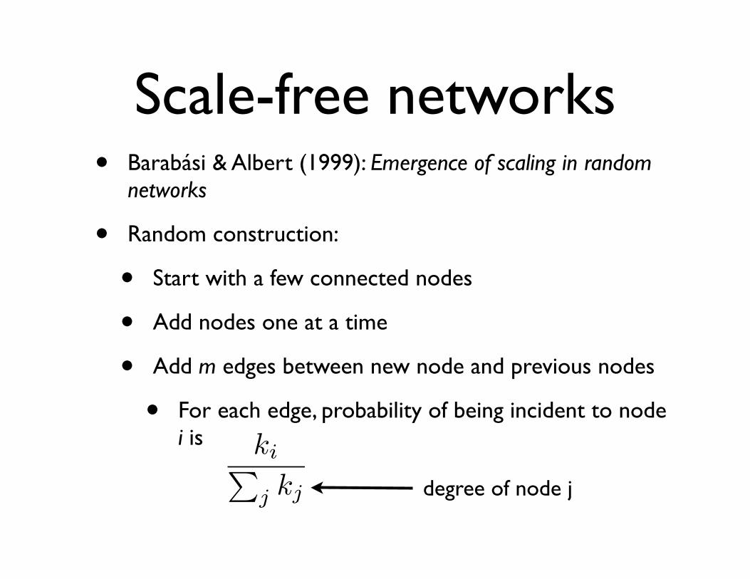
Scale-free networks• Barabási & Albert (1999): Emergence of scaling in random

networks

• Random construction:

• Start with a few connected nodes

• Add nodes one at a time

• Add m edges between new node and previous nodes

• For each edge, probability of being incident to node i is ki�

j kj degree of node j

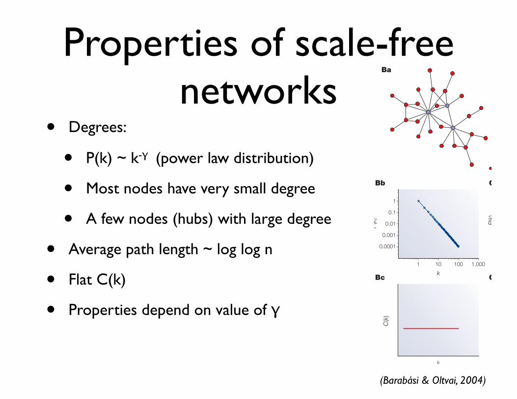
Properties of scale-free networks

• Degrees:

• P(k) ~ k-γ (power law distribution)

• Most nodes have very small degree

• A few nodes (hubs) with large degree

• Average path length ~ log log n

• Flat C(k)

• Properties depend on value of γ


R E V I EW S






A Random network

Ab

Ac

Aa

Bb

Bc

Ba

Cb

Cc

Ca


1

0.1

0.01

0.001

0.0001

1 10 100 1,000

P(k

)C

(k)

k k

kk k

P(k

)

P(k

)

100

10

10–1

10–2

10–3

10–4

10–5

10–6

10–7

10–8

100 1,000 10,000

C(k

)

log

C(k

)

log k


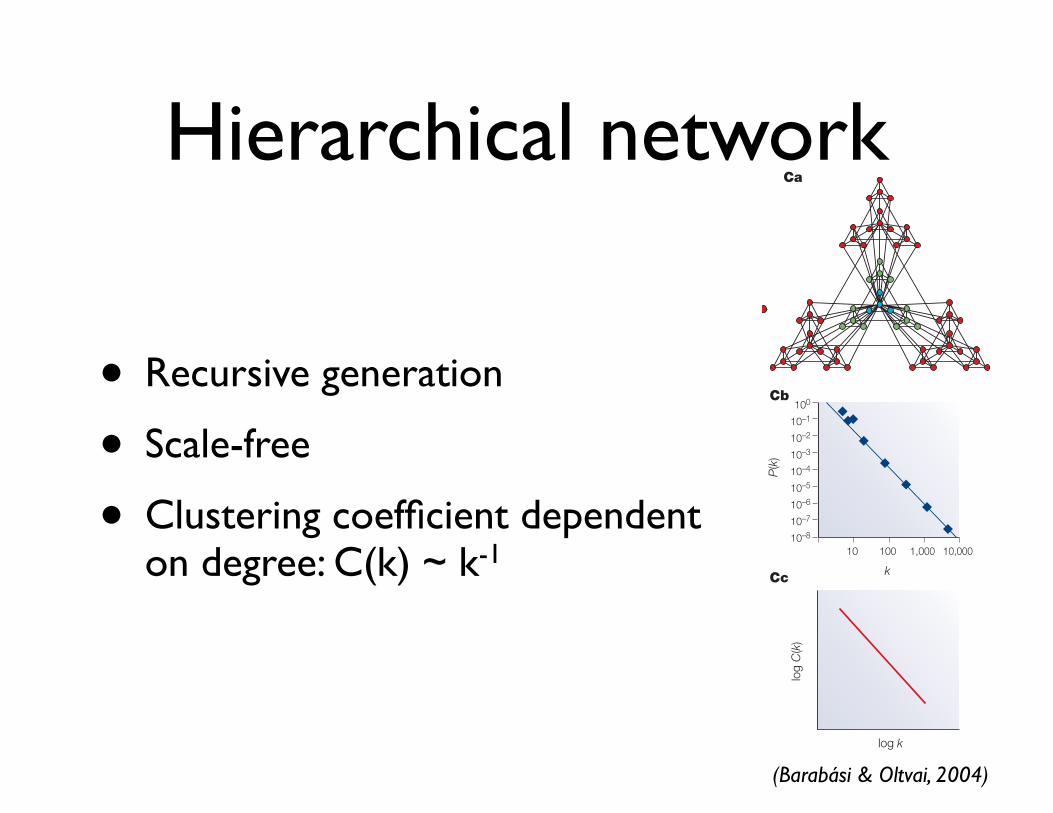
Hierarchical network

• Recursive generation

• Scale-free

• Clustering coefficient dependent on degree: C(k) ~ k-1


R E V I EW S






A Random network

Ab

Ac

Aa

Bb

Bc

Ba

Cb

Cc

Ca


1

0.1

0.01

0.001

0.0001

1 10 100 1,000

P(k

)C

(k)

k k

kk k

P(k

)

P(k

)

100

10

10–1

10–2

10–3

10–4

10–5

10–6

10–7

10–8

100 1,000 10,000

C(k

)

log

C(k

)

log k


Classifying networks

• Metabolic networks

• scale-free

• PPI networks

• scale-free

• Regulatory networks

• mixed

• out-degree of transcription factors is scale-free

• in-degree of regulated genes is exponential

Paths in biological networks

• Path length between two vertices is often very small

• random graph gives expected path length as log N

• scale-free graph has log log N expected path length

• However, hubs not often connected to each other: disassortative

Small-world networks

• Small-world networks are graphs with small average path length

• ER graphs are small-world: log n average path length

• Scale-free graphs often very small: log log n (for some values of ϒ)

• However, biological networks are both small-world and disassortative: hubs are not often connected to each other

Evolving networks• Growth

• Early nodes have more links

• Preferential attachment

• As new nodes added, more likely to be connected to already highly-connected nodes

• Leads to scale-free networks

• Gene duplication

• Major force in protein network evolution

• Highly-connected nodes more likely to have neighbors duplicate and add more edges

Network problems• Network inference

• Given raw experimental data

• Infer network structure

• Motif finding

• Identify common subgraph topologies

• Module detection

• Identify subgraphs that perform same function

• Conserved modules

• Identify modules that are shared in networks of multiple species

Network motifs

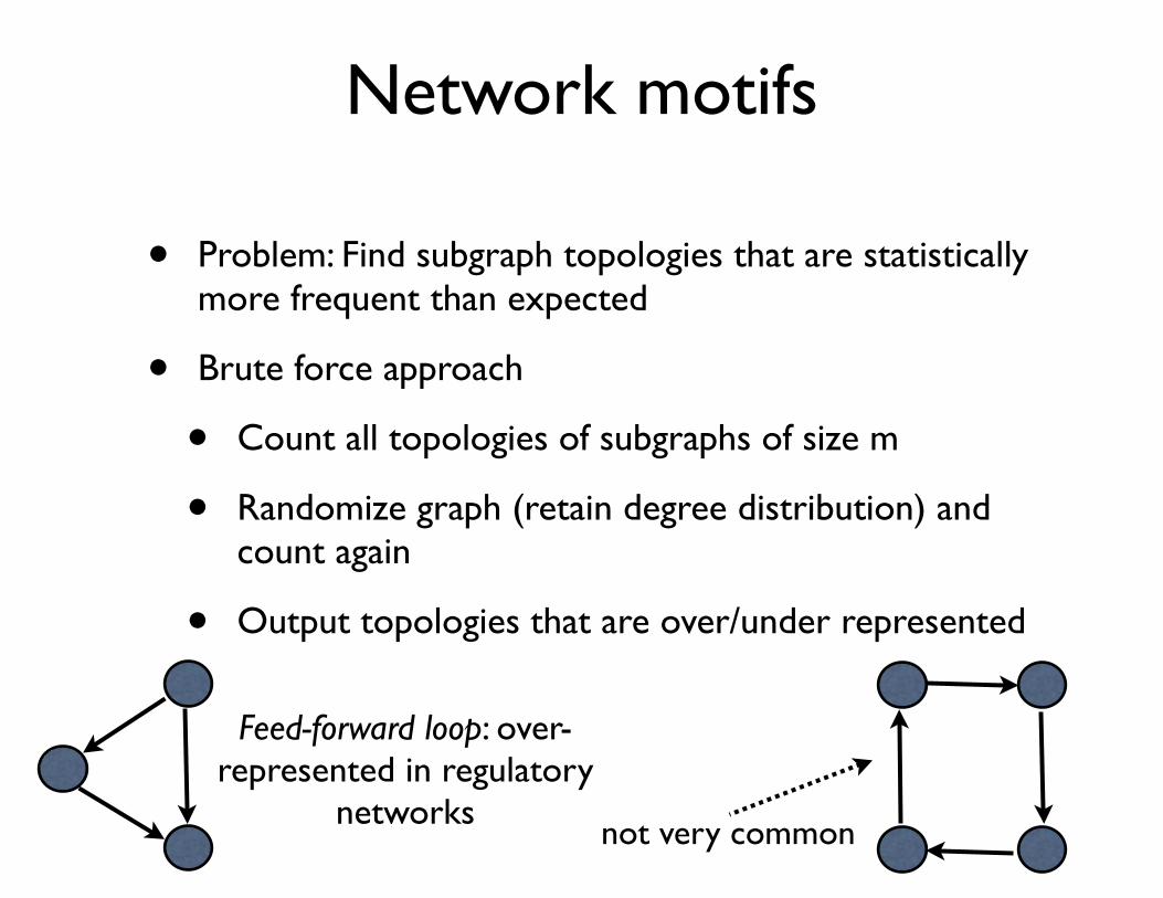
• Problem: Find subgraph topologies that are statistically more frequent than expected

• Brute force approach

• Count all topologies of subgraphs of size m

• Randomize graph (retain degree distribution) and count again

• Output topologies that are over/under represented

Feed-forward loop: over-represented in regulatory

networksnot very common

Network modules

• Modules: dense (highly-connected) subgraphs (e.g., large cliques or partially incomplete cliques)

• Problem: Identify the component modules of a network

• Difficulty: definition of module is not precise

• Hierarchical networks have modules at multiple scales

• At what scale to define modules?

Conserved modules

• Identify modules in multiple species that have “conserved” topology

• Typical approach:

• Use sequence alignment to identify homologous proteins and establish correspondence between networks

• Using correspondence, output subsets of nodes with similar topology

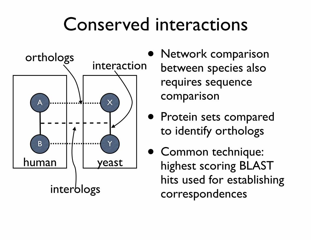
Conserved interactions

• Network comparison between species also requires sequence comparison

• Protein sets compared to identify orthologs

• Common technique: highest scoring BLAST hits used for establishing correspondences

Y

X

B

A

human yeast

orthologs

interologs

interaction

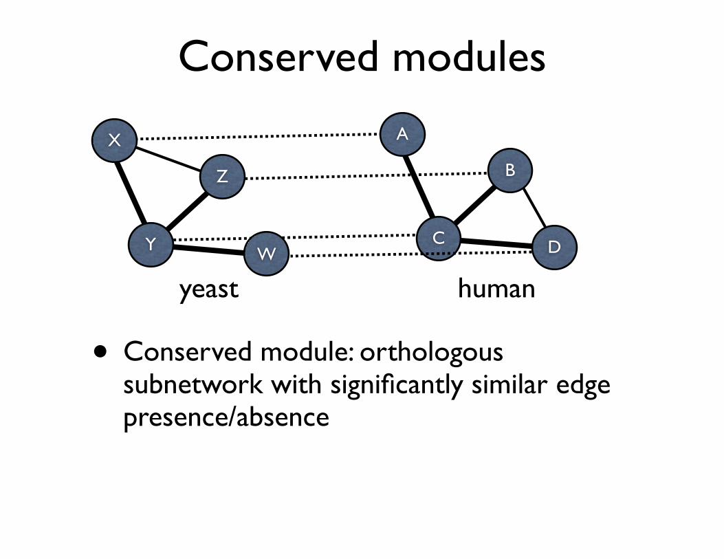
Conserved modules

• Conserved module: orthologous subnetwork with significantly similar edge presence/absence

Y

X

Z

WC

A

B

D

humanyeast

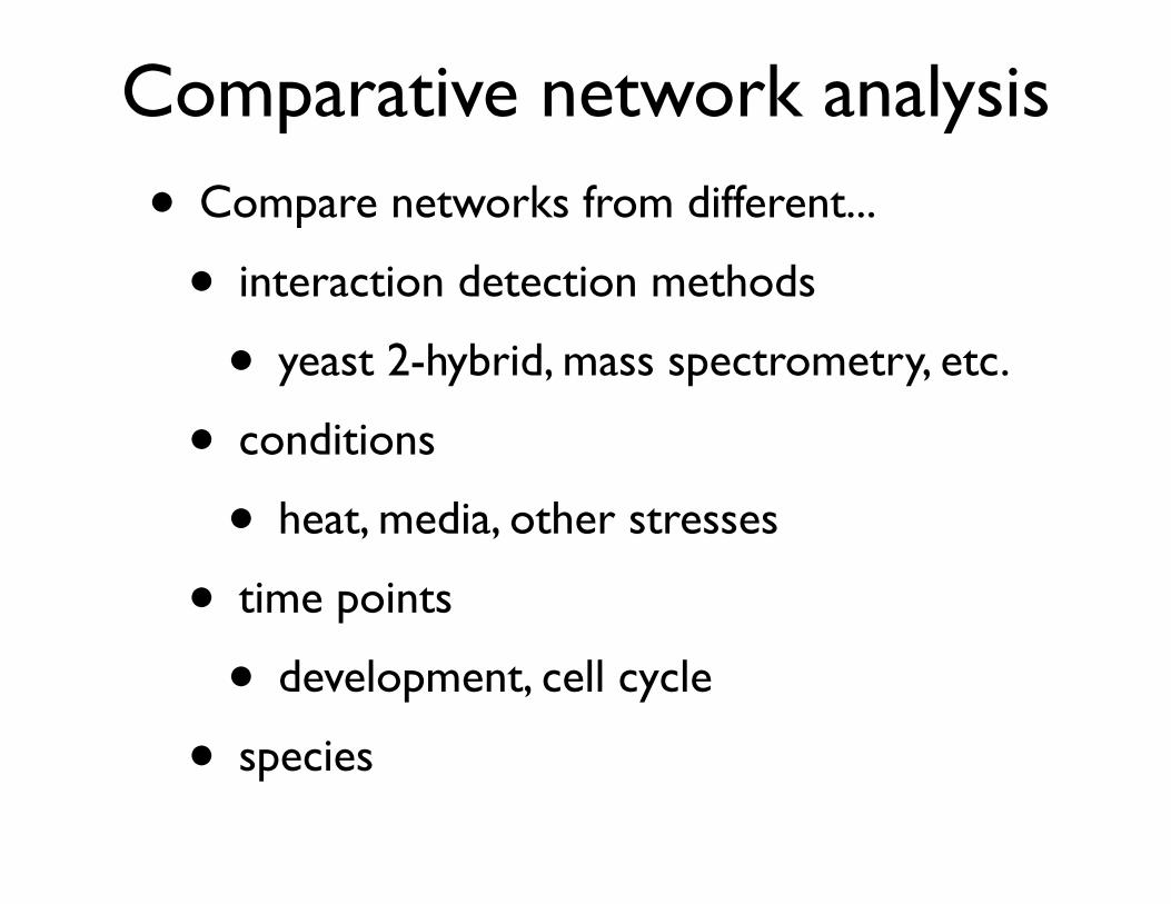
Comparative network analysis

• Compare networks from different...

• interaction detection methods

• yeast 2-hybrid, mass spectrometry, etc.

• conditions

• heat, media, other stresses

• time points

• development, cell cycle

• species

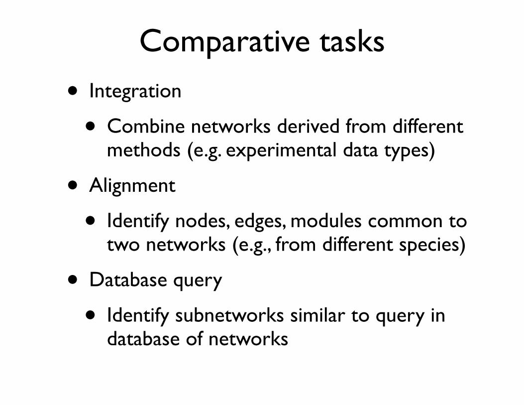
Comparative tasks

• Integration

• Combine networks derived from different methods (e.g. experimental data types)

• Alignment

• Identify nodes, edges, modules common to two networks (e.g., from different species)

• Database query

• Identify subnetworks similar to query in database of networks

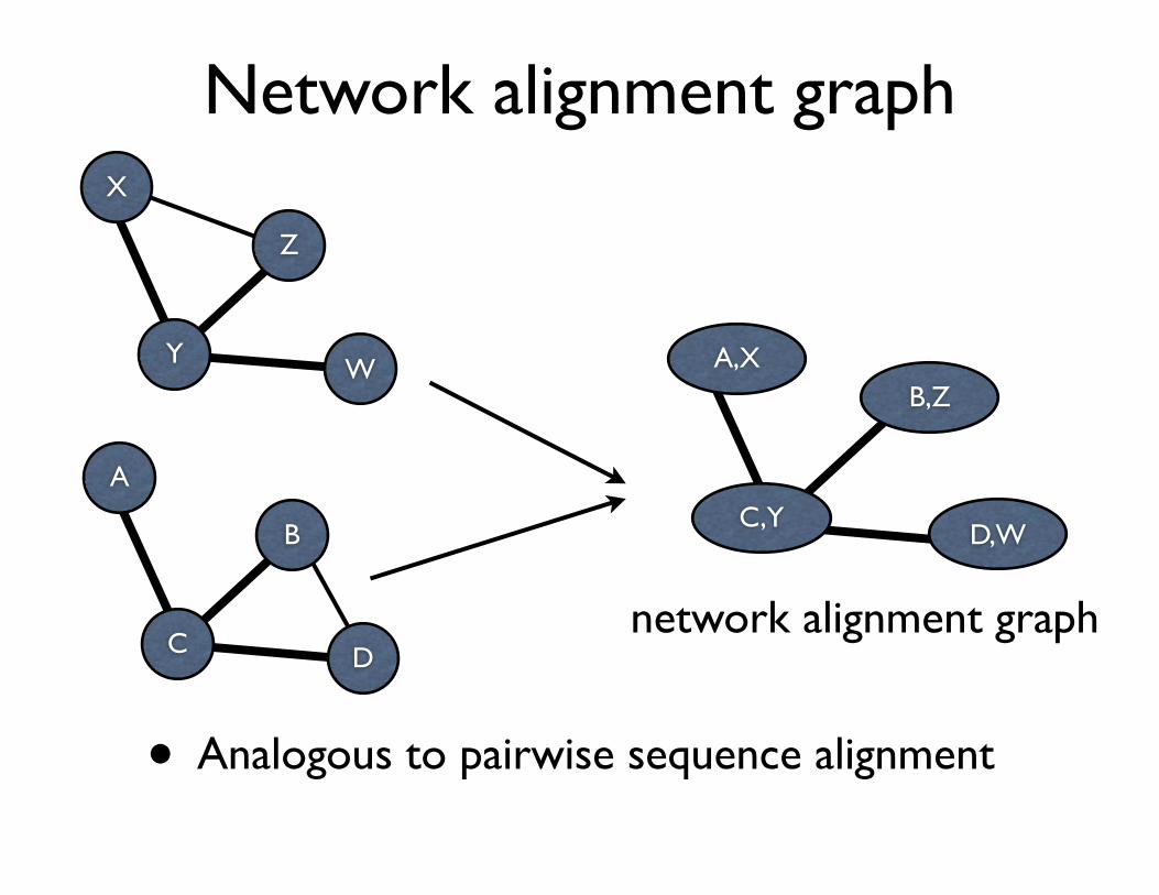
Network alignment graph

• Analogous to pairwise sequence alignment

Y

X

Z

W

C

A

B

D

A,XB,Z

D,WC,Y

network alignment graph

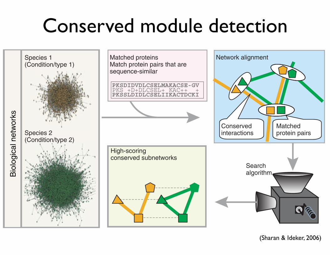
Conserved module detection

428 VOLUME 24 NUMBER 4 APRIL 2006 NATURE BIOTECHNOLOGY

involving either two genes or two proteins in one species and their best sequence matches in another species. Beyond alignment of single inter-actions, it is possible to envisage a whole array of network structures that might be conserved between two protein networks. For instance, conserved linear paths may correspond to signaling pathways, and con-served clusters of interactions may be indicative of protein complexes. In certain cases, for example, when the two networks being compared represent linear chains of interactions24, the network alignment problem admits efficient algorithmic solutions. In general, the problem is com-putationally hard (generalizing subgraph isomorphism under certain formulations), but heuristic approaches have been devised for it (e.g., Berg & Lassig25).

One heuristic approach creates a merged representation of the two networks being compared, called a network alignment graph, and then applies a greedy algorithm for identifying the conserved subnetworks embedded in the merged representation. In a network alignment graph, the nodes represent sets of molecules, one from each network, and the links represent conserved molecular interactions across the different net-works (Fig. 1). The alignment is particularly simple when there exists a one-to-one correspondence between molecules across the two networks, but in general there may be a complex many-to-many correspondence.

A network alignment graph facilitates the search for conserved network regions, as these will appear as subnetworks with specific

structure. For instance, conserved protein complexes might appear as clusters of densely interacting nodes. This technique was first used by Ogata et al.26, who searched for correspondences between the reactions of specific metabolic pathways and the genomic locations of the genes encoding the enzymes catalyzing those reactions. Their network align-ment graph combined the genome ordering information, represented as a network of genes arranged in a linear (or circular) path, with a network of successive enzymes in metabolic pathways. Single-linkage clustering was applied to this graph to identify pathways for which the enzymes clustered along the genome (Fig. 2a).

Kelley et al.18 applied the concept of network alignment to the study of protein interaction networks. They translated the problem of find-ing conserved pathways to that of finding high-scoring paths in the alignment graph. Their algorithm, PathBLAST, identified five regions that were conserved across the protein networks of Saccharomyces cerevisiae and Helicobacter pylori. This comparison was later extended to detect conserved protein clusters rather than paths27, employing a likelihood-based scoring scheme that weighs the denseness of a given subnetwork versus the chance of observing such topology at random (Box 1). The latter approach was recently used by Suthram et al.28 to show that the protein-protein interaction network of Plasmodium fal-ciparum differs substantially from those of other eukaryotes. Finally, Koyuturk et al.29 developed an evolution-based scoring scheme to

detect conserved protein clusters, which takes into account interaction insertion/deletion and protein duplication events (Box 1). Their MaWish algorithm was applied to detect human-mouse conserved subnetworks.

The methodology of network align-ment can also be applied to predict vari-ous properties of genes and proteins on a global scale. First and foremost, a conserved subnetwork that contains many proteins of the same known function suggests that the remaining proteins also have that function. We have recently used this concept to pre-dict thousands of new protein functions for yeast, worm (Caenorhabditis elegans) and fly (Drosophila melanogaster), with an estimated success rate of 58–63% (ref. 13). More com-plex relationships, such as protein interac-tions, functional orthology and links between cellular processes, can also be inferred from the network alignment13,30,31.

Multiple network alignmentThe generalization of the network alignment process to more than two networks entails devising an appropriate scoring scheme and

Table 1 Modes of network comparisonMode Common application Main goals Some current limitations

Alignment At least two networks of the same type across species

Identification of functional (conserved) protein modules; study of network evolution; interaction prediction

Limited to few (five or fewer) species; nonevolu-tion-based scores

Integration At least two networks of different types for the same species

Identification of modules (supported by several networks); study of interrelations between data types; interaction prediction

No agreed-upon way to combine scores over dif-ferent networks

Querying Subnetwork module versus a network Identification of duplicated/conserved instances of the module; knowledge transfer

Query is limited to a tree topology; nonevolution-based scores

Conservedinteractions

Matchedprotein pairs

High-scoringconserved subnetworks

Searchalgorithm

Matched proteinsMatch protein pairs that aresequence-similar

Species 1(Condition/type 1)

Species 2(Condition/type 2)

Network alignment

PKSDIDVDLCSELMAKACSE-GVPKS +D+DLCSEL+ KAC++ +PKSSLDIDLCSELIIKACTDCKI

Bio

logi

cal n

etw

orks

Figure 1 Network alignment. Network alignment combines protein interaction data that are available for each of at least two species with orthology information based on the corresponding protein sequences. A detailed probabilistic model is used to identify protein subnetworks within the aligned network that are conserved across the species. Each node in this aligned network represents a set of sequence-similar proteins (one from each species) and each link represents a conserved interaction. Other than species, the networks being compared can also be sampled across different biological conditions or interaction types.

REV IEW

©2

006 N

atu

re P

ub

lis

hin

g G

rou

p

htt

p:/

/ww

w.n

atu

re.c

om

/natu

reb

iote

ch

no

log

y

(Sharan & Ideker, 2006)

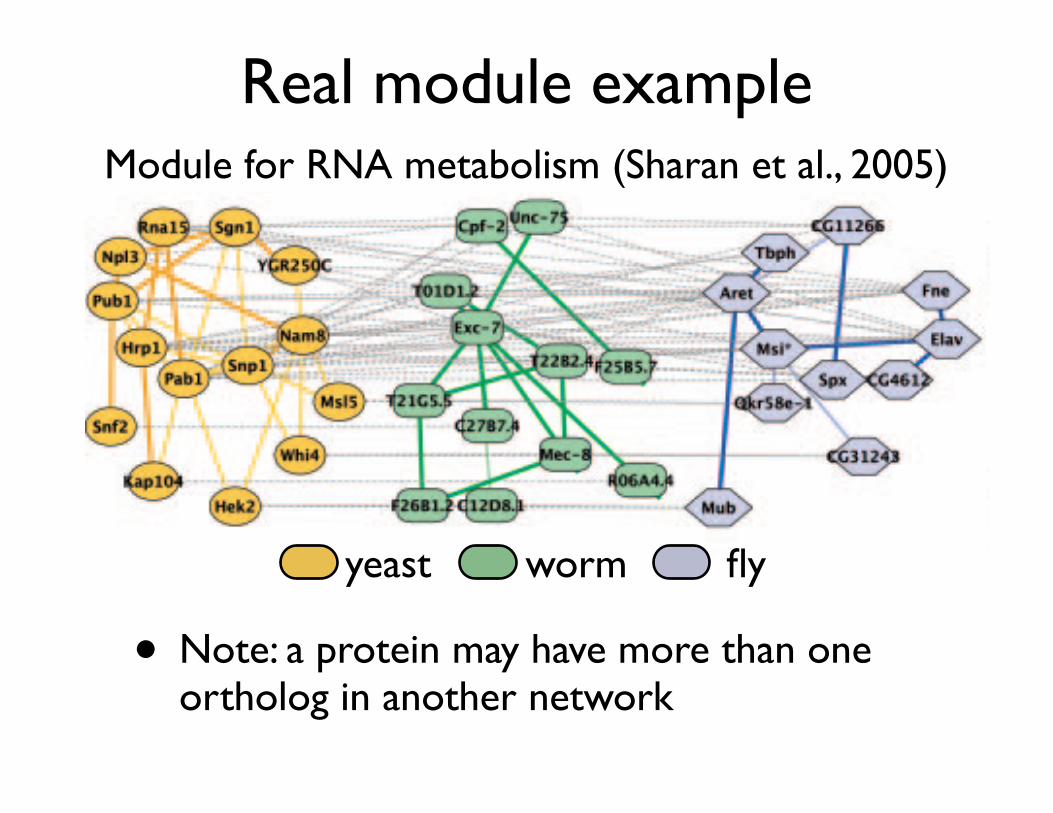
Real module example

• Note: a protein may have more than one ortholog in another network

Prediction of Protein Interactions. We also used the multiple networkalignment to predict protein–protein physical interactions. Wepredicted an interaction between a pair of proteins based on (i)

evidence that proteins with similar sequences interact within otherspecies (directly or by a common network neighbor) and, optionally,(ii) cooccurrence of these proteins in the same conserved cluster or

Fig. 2. Representative conserved network regions. Shown are conserved clusters (a–k) and paths (l and m) identified within the networks of yeast, worm, andfly. Each region contains one or more overlapping clusters or paths (see Fig. 3). Proteins from yeast (orange ovals), worm (green rectangles), or fly (blue hexagons)are connected by direct (thick line) or indirect (connection via a common network neighbor; thin line) protein interactions. Horizontal dotted gray links indicatecross-species sequence similarity between proteins (similar proteins are typically placed on the same row of the alignment). Automated layout of networkalignments was performed by using a specialized plug-in to the CYTOSCAPE software (34) as described in Supporting Text.

1976 ! www.pnas.org"cgi"doi"10.1073"pnas.0409522102 Sharan et al.

yeast worm fly

Module for RNA metabolism (Sharan et al., 2005)

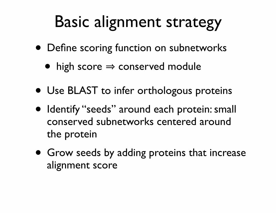
Basic alignment strategy

• Define scoring function on subnetworks

• high score ⇒ conserved module

• Use BLAST to infer orthologous proteins

• Identify “seeds” around each protein: small conserved subnetworks centered around the protein

• Grow seeds by adding proteins that increase alignment score

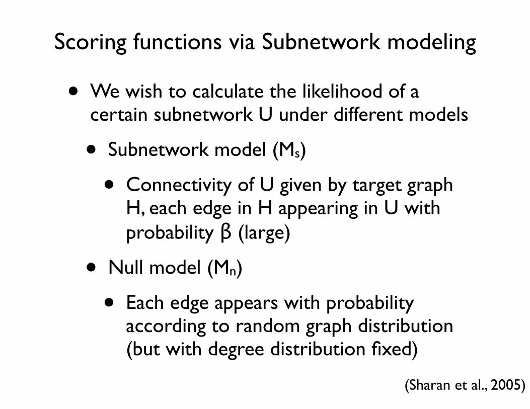
Scoring functions via Subnetwork modeling

• We wish to calculate the likelihood of a certain subnetwork U under different models

• Subnetwork model (Ms)

• Connectivity of U given by target graph H, each edge in H appearing in U with probability β (large)

• Null model (Mn)

• Each edge appears with probability according to random graph distribution (but with degree distribution fixed)

(Sharan et al., 2005)

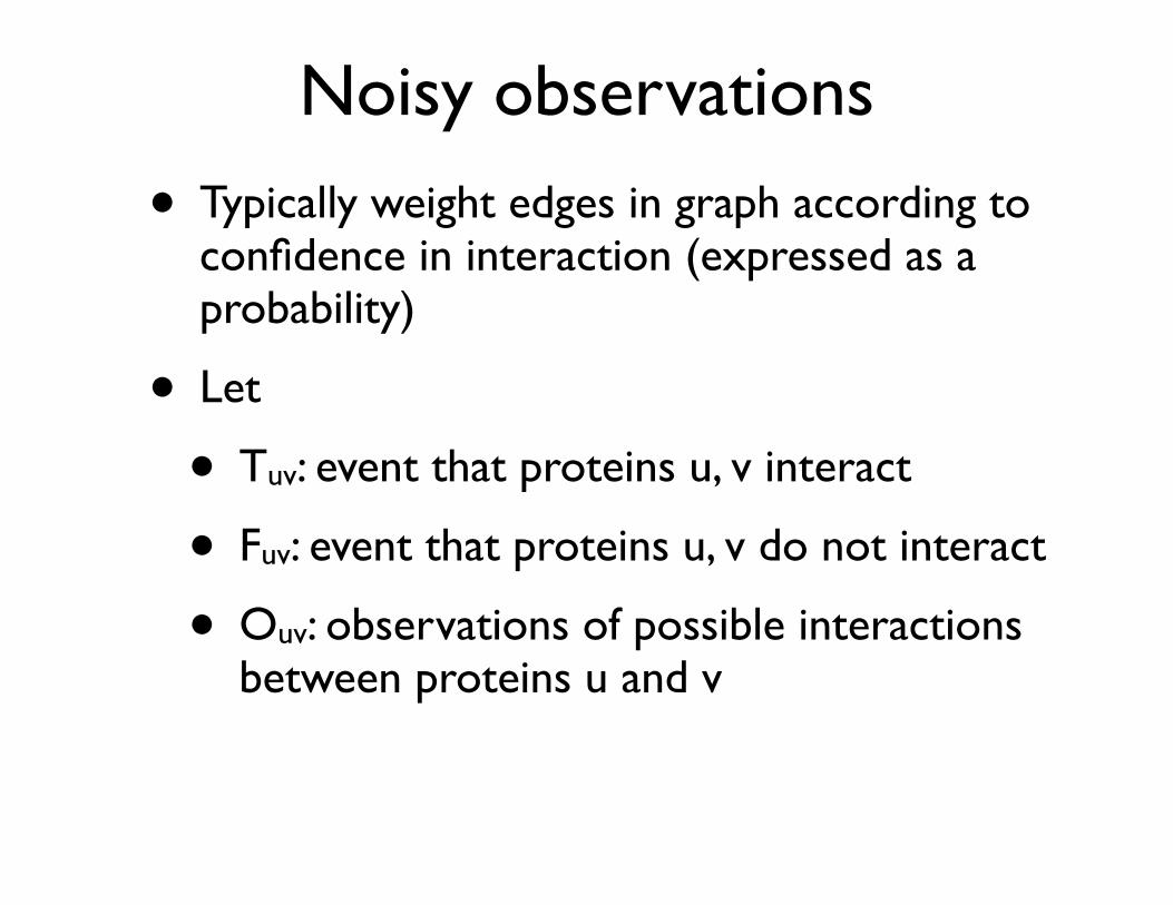
Noisy observations

• Typically weight edges in graph according to confidence in interaction (expressed as a probability)

• Let

• Tuv: event that proteins u, v interact

• Fuv: event that proteins u, v do not interact

• Ouv: observations of possible interactions between proteins u and v

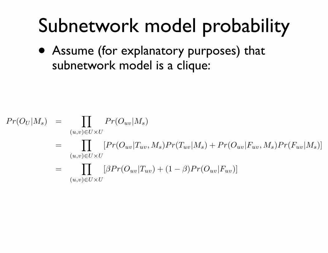
Subnetwork model probability• Assume (for explanatory purposes) that

subnetwork model is a clique:

Pr(OU |Ms) =�

(u,v)⇥U�U

Pr(Ouv|Ms)

=�

(u,v)⇥U�U

[Pr(Ouv|Tuv,Ms)Pr(Tuv|Ms) + Pr(Ouv|Fuv,Ms)Pr(Fuv|Ms)]

=�

(u,v)⇥U�U

[�Pr(Ouv|Tuv) + (1� �)Pr(Ouv|Fuv)]

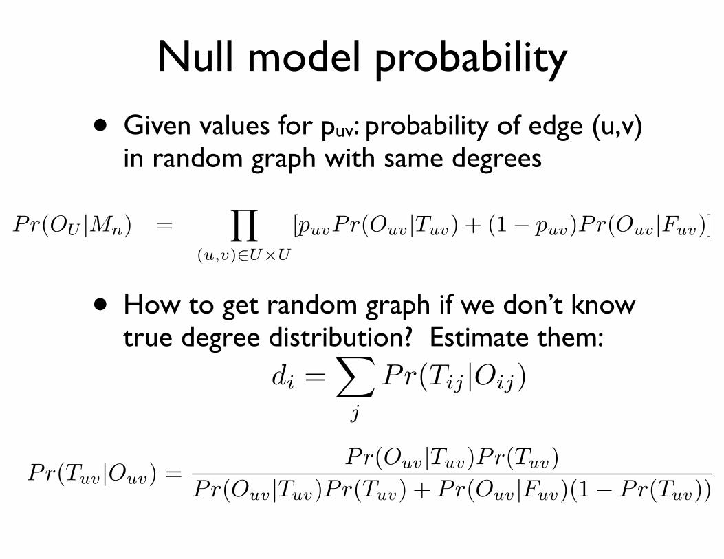
Null model probability

• Given values for puv: probability of edge (u,v) in random graph with same degrees

• How to get random graph if we don’t know true degree distribution? Estimate them:

Pr(OU |Mn) =�

(u,v)⇥U�U

[puvPr(Ouv|Tuv) + (1� puv)Pr(Ouv|Fuv)]

di =�

j

Pr(Tij |Oij)

Pr(Tuv|Ouv) =Pr(Ouv|Tuv)Pr(Tuv)

Pr(Ouv|Tuv)Pr(Tuv) + Pr(Ouv|Fuv)(1� Pr(Tuv))

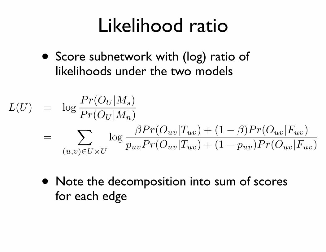
Likelihood ratio

• Score subnetwork with (log) ratio of likelihoods under the two models

• Note the decomposition into sum of scores for each edge

L(U) = logPr(OU |Ms)Pr(OU |Mn)

=�

(u,v)⇥U�U

log�Pr(Ouv|Tuv) + (1� �)Pr(Ouv|Fuv)

puvPr(Ouv|Tuv) + (1� puv)Pr(Ouv|Fuv)

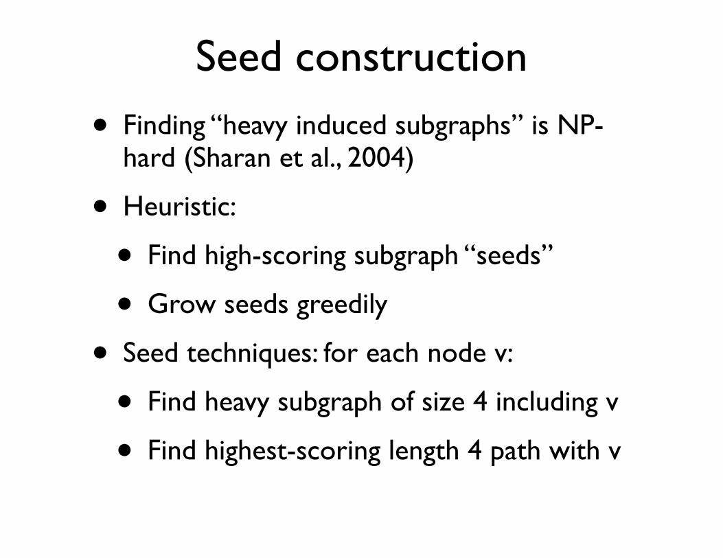
Seed construction

• Finding “heavy induced subgraphs” is NP-hard (Sharan et al., 2004)

• Heuristic:

• Find high-scoring subgraph “seeds”

• Grow seeds greedily

• Seed techniques: for each node v:

• Find heavy subgraph of size 4 including v

• Find highest-scoring length 4 path with v

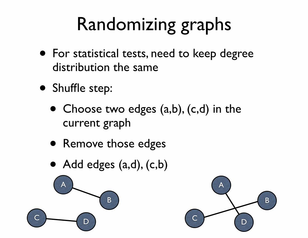
Randomizing graphs

• For statistical tests, need to keep degree distribution the same

• Shuffle step:

• Choose two edges (a,b), (c,d) in the current graph

• Remove those edges

• Add edges (a,d), (c,b)

C

A

B

D C

A

B

D

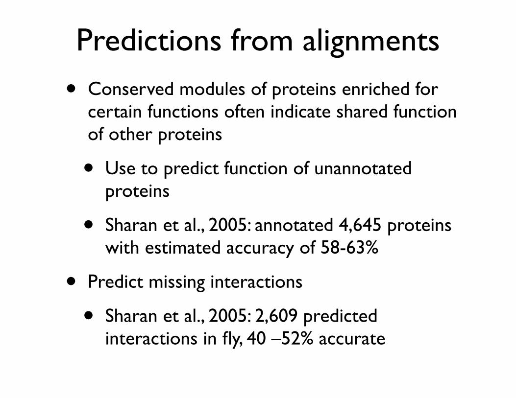
Predictions from alignments

• Conserved modules of proteins enriched for certain functions often indicate shared function of other proteins

• Use to predict function of unannotated proteins

• Sharan et al., 2005: annotated 4,645 proteins with estimated accuracy of 58-63%

• Predict missing interactions

• Sharan et al., 2005: 2,609 predicted interactions in fly, 40 –52% accurate

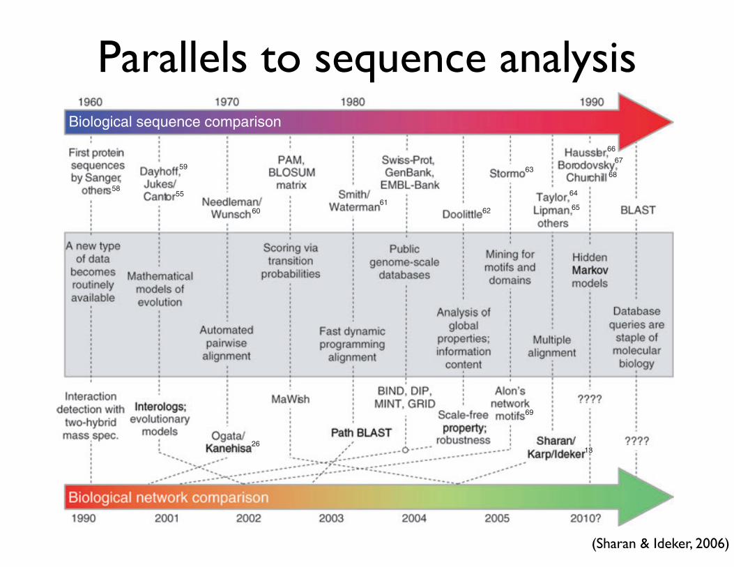
Parallels to sequence analysis

NATURE BIOTECHNOLOGY VOLUME 24 NUMBER 4 APRIL 2006 431

Network queryingNetwork alignment and integration are focused on de novo discovery of biologically significant regions embedded in a network, based on the assumption that regions supported by multiple networks are functional. In contrast, a super-vised approach to the module detection problem relies on a query subnetwork that is previously known to be functional. The goal is to identify subnetworks in a given network that are similar to the query. Kelley et al.18 approached the query problem in the context of the PathBLAST net-work alignment algorithm, by designating one of the networks as the query. When PathBLAST is applied in this setting, it identifies all matches to the query in the network under study. As in the comparison case, the treatment here is only in queries that take the form of a linear path of interacting proteins.

Recently, Pinter et al.44 devised an algorithm for querying metabolic networks. Their algo-rithm allows querying metabolic pathways that take the form of a tree within a collection of such pathways. Figure 2d shows an example of their approach: here, a query of a core pathway revealed an allantoin degradation pathway in E. coli and a ureide degradation pathway in yeast.

Network querying tools are still at an early stage and are currently limited to sparse topolo-gies, such as paths and trees. Approaches to handle more general queries could benefit from the rich literature on graph mining techniques in the data mining community31,45.

Network evolutionUnderstanding how networks evolve is a fundamental issue, which affects each of the above analysis modes as well as the study of networks in gen-eral. Two kinds of processes have been invoked to explain network evolu-tion. The first consists of sequence mutations in a gene, which result in modifications of the interface between interacting proteins46 (Fig. 3a). Consequently, the corresponding protein may gain new connections (attachment) or lose (detachment) some of the existing connections to other proteins. The second type of evolutionary process consists of gene duplication, followed by either silencing of one of the duplicated genes or by functional divergence of the duplicates (Fig. 3b). In terms of the network, a gene duplication corresponds to the addition of a node with links identical to the original node, followed by the divergence of some of the redundant links between the two duplicate nodes.

Berg et al.47 referred to link attachment and detachment processes collectively as link dynamics. They estimated the empirical rates of link dynamics and gene duplication in the yeast protein network, finding the former to be at least one order of magnitude higher than the latter. Based on this observation, they proposed a model for the evolution of pro-tein networks in which link dynamics are the major evolutionary forces shaping the topology of the network, whereas slower gene duplication processes mainly affect its size. Rzhetsky & Gomez48 formulated a model that uses these two evolutionary processes, but whose underlying basic elements are domains rather than whole proteins. Barabasi & Albert49 suggested gene duplication as the major mechanism for generating the scale-free topology of protein interaction networks. Their network growth model predicts that molecules that appeared early in the network are the most connected ones. Several lines of empirical evidence sup-

port this hypothesis: metabolites of some of the most ancient pathways, such as glycolysis and the tricarboxylic acid cycle, are among the most connected substrates in metabolic networks50; for protein interaction networks, one observes a positive correlation between the evolutionary age of a protein and its degree of connectivity51.

Network comparison: the next ten years?Notwithstanding the recent advances, the field of network comparison is still very young. However, by exploiting the close analogy to sequence comparison, one can envision some of the key milestones on the road ahead (Fig. 4). Methods for sequence comparison have been the main focus of bioinformatics for most of its history, starting in 1970 with the publication of the first comparison algorithm by Needleman & Wunsch52. Since that initial work, major advances have included bet-ter alignment score functions to more accurately reflect evolutionary distance, methods for multiple sequence alignment and numerous opti-mizations to the search algorithm (Fig. 4). In recent years, the develop-ment of sequence analysis tools has been largely driven by the immense amounts of data emerging from the human genome53,54 and other sequencing projects.

Unlike the more mature field of sequence alignment, network alignment has a conceptual framework and several proof-of-prin-ciple studies, but relatively little in terms of advanced computational methodology. Nevertheless, it is exciting that virtually all of the major advances that occurred for sequence alignment can be envisioned for network alignment. For instance, a clear parallel goal is to prog-ress from pairwise to multiple alignment of networks. At present, a method for three-species network alignment has been described (see above discussion of Sharan et al.13), but this algorithm scales poorly with the number of networks/species and may reach a practi-cal limit at four or five. As yet another example, save perhaps a single study29, the score functions for assessing network similarity are not

Biological sequence comparison

58

59

55

6061

62

63

64

65

66

67

68

69

2613

Figure 4 Parallels between sequence and network comparison on a timeline. The recent and possibly future developments in methods for network comparison are shown in the context of the analogous developments as they occurred in the field of sequence comparison. General milestones for both fields are shown in the middle (gray box), with the specific instances for sequence versus network comparison appearing directly above or below, respectively.

REV IEW

©2006 N

atu

re P

ub

lish

ing

Gro

up

h

ttp

://w

ww

.natu

re.c

om

/natu

reb

iote

ch

no

log

y

(Sharan & Ideker, 2006)

Documents

cellular network analysis - University of Wisconsin–Madison