Embed Size (px)
Citation preview
1
Journal of ICT, 18, No. 1 (January) 2019, pp: 1–18
How to cite this paper:
Tran, Q. T., Li, H., & Trinh, Q. K. (2019). Cellular network traffic prediction using exponential smoothing Methods. Journal of Information and Communication Technology, 18 (1), 1-18.
CELLULAR NETWORK TRAFFIC PREDICTION USING EXPONENTIAL SMOOTHING METHODS 1,2Quang Thanh Tran, 1Li Hao & 2Quang Khai Trinh
1Key Lab of Information Coding and Transmission, Southwest Jiaotong University, China
2Faculty of Electrical-Electronic Engineering, University of Transport and Communications, Vietnam
[email protected]; [email protected]; [email protected]
ABSTRACT
Wireless traffic prediction plays an important role in network planning and management, especially for real-time decision making and short-term prediction. Systems require high accuracy, low cost, and low computational complexity prediction methods. Although exponential smoothing is an effective method, there is a lack of use with cellular networks and research on data traffic. The accuracy and suitability of this method need to be evaluated using several types of traffic. Thus, this study introduces the application of exponential smoothing as a method of adaptive forecasting of cellular network traffic for cases of voice (in Erlang) and data (in megabytes or gigabytes). Simple and Error, Trend, Seasonal (ETS) methods are used for exponential smoothing. By investigating the effect of their smoothing factors in describing cellular network traffic, the accuracy of forecast using each method is evaluated. This research comprises a comprehensive analysis approach using multiple case study comparisons to determine the best fit model. Different exponential smoothing models are evaluated for various traffic types in different time scales. The experiments are implemented on real data from a commercial cellular network, which is divided into a training data part for modeling and test data part for forecasting comparison.
Received: 30 January 2018 Accepted: 15 October 2018 Published: 11 December 2018

Journal of ICT, 18, No. 1 (January) 2019, pp: 1–18
2
This study found that ETS framework is not suitable for hourly voice traffic, but it provides nearly the same results with Holt–Winter’s multiplicative seasonal (HWMS) in both cases of daily voice and data traffic. HWMS is presumably encompassed by ETC framework and shows good results in all cases of traffic. Therefore, HWMS is recommended for cellular network traffic prediction due to its simplicity and high accuracy.
Keywords: Cellular network traffic, exponential smoothing, Holt–Winter’s multiplicative seasonal, wireless traffic prediction.
INTRODUCTION
Wireless traffic prediction is a key component of network planning, development, and management. Accurate prediction will become even more necessary with the development of 5th generation wireless systems (5G) that contain many new service capabilities (5G PPP, 2015). The 5G system has a higher capacity and higher density of mobile broadband users than the current 4G system. It also supports device-to-device communications and massive machine-type communications (NGMN Alliance, 2015). Consequently, people are living in the age of social networks (Tyagi & Kumar, 2017) and the Internet-of-Things (Matta, Pant, & Arora, 2017). Life becomes more convenient and intelligent when everything can be connected via heterogeneous wireless networks (Qiang, Li, & Altman, 2017). Along with these advanced technologies, Yusuf-Asaju, Dahalin, and Ta’a (2018) also figured out the issues of mobile network performance and proposed a framework for modeling mobile network quality of experience using the big data analytics approach. And in fact, better network operation and management are required to ensure a robust infrastructure that includes the underlying network and supporting technologies, for example.
Analysis of wireless network traffic shows that the traffic series normally contains seasonal components and can be modeled and forecasted by time series analysis models (Tran, Ma, Li, Hao, & Trinh, 2015). Authors in these papers proposed combining statistical procedures for modeling and forecasting cellular network traffic, such as the autoregressive integrated moving average (ARIMA) and generalized autoregressive conditional heteroskedasticity (GARCH). They took advantage of the ARIMA model for capturing the conditional mean of the traffic series and the GARCH model for dealing with the conditional heteroskedasticity existing inside the traffic. They achieved better forecast results compared with the individual models, but at the cost of computational complexity. The results can be used for capacity planning and overload warning issues that are important parts of network planning.
Exponential smoothing is a simple method of adaptive forecasting in which the forecasts adjust based on past errors, unlike forecasts from regression models that use fixed coefficients. Exponential smoothing

3
Journal of ICT, 18, No. 1 (January) 2019, pp: 1–18
methods have been applied in several areas, such as palm oil real production forecasting (Siregar, Butar-Butar, Rahmat, Andayani, & Fahmi, 2017), power (Usaratniwart, Sirisukprasert, Hatti, & Hagiwara, 2017), revenue forecasting (Rahman, Salma, Hossain, & Khan, 2016), and solar irradiance prediction (Margaret & Jose, 2015), to name a few. These researchers all achieved good results with this low-complexity and low-cost method. In terms of wireless traffic prediction, Tikunov and Nishimura (2007) proposed the application of Holt–Winter’s exponential smoothing, which is simple, low cost, does not require a without highly skilled analyst, and operates nearly automatically for GSM/GPRS network Erlang traffic prediction. The recorded data were classified into three types, namely high, medium, and low intensity traffic cells. The authors focused on cells with high and medium traffic intensity for the purposes of overload warning and capacity planning. Although good results were achieved, only voice traffic was considered. In the era of data, there is a necessity for more comprehensive studies about using exponential smoothing in cellular network traffic that includes not only voice (Erlang) but also data (megabytes or gigabytes).
Base on the mentioned requirement, more exponential smoothing methods were investigated that included not only the specific Holt–Winter’s multiplicative seasonal method (HWMS), but also different types of exponential smoothing methods. They were then applied to forecast cellular network traffic that consists of not only voice (in Erlang) but also data (in megabytes or gigabytes). In this study, the simple exponential smoothing methods include single, double, Holt–Winter’s no seasonal, Holt–Winter’s additive seasonal, and HWMS. The methods are introduced together with an Error, Trend, Seasonal (ETS) framework. The exponential smoothing methods are considered in three cases of hourly voice, daily voice, and daily data traffic types.
SIMPLE EXPONENTIAL SMOOTHING
Simple exponential smoothing methods include:
Single smoothing: one parameter -
Double smoothing: one parameter -
Holt-Winters – No seasonal: two parameters -
Holt-Winters – Additive seasonal: three parameters and-
Holt-Winters – Multiplicative seasonal: three parameters -
where α, β, and γ are the damping, or smoothing, factors.
3
Base on the mentioned requirement, more exponential smoothing methods were investigated that included not
only the specific Holt–Winter’s multiplicative seasonal method (HWMS), but also different types of
exponential smoothing methods. They were then applied to forecast cellular network traffic that consists of not
only voice (in Erlang) but also data (in megabytes or gigabytes). In this study, the simple exponential
smoothing methods include single, double, Holt–Winter’s no seasonal, Holt–Winter’s additive seasonal, and
HWMS. The methods are introduced together with an Error, Trend, Seasonal (ETS) framework. The
exponential smoothing methods are considered in three cases of hourly voice, daily voice, and daily data traffic
types.
SIMPLE EXPONENTIAL SMOOTHING
Simple exponential smoothing methods include:
- Single smoothing: one parameter 0 < 𝛼 ≤ 1,
- Double smoothing: one parameter 0 < 𝛼 ≤ 1,
- Holt-Winters – No seasonal: two parameters 0 < 𝛼,𝛽 < 1,
- Holt-Winters – Additive seasonal: three parameters 0 < 𝛼,𝛽, 𝛾 < 1, and
- Holt-Winters – Multiplicative seasonal: three parameters 0 < 𝛼,𝛽, 𝛾 < 1
where α, β, and γ are the damping, or smoothing, factors.
The analysis of cellular network traffic is appropriate for the HWMS method (Valakevicius &
Brazenas, 2015), which is suitable for a series with a linear time trend and multiplicative seasonal
variation. If xt is the input traffic series, then the smoothed series, 𝑥�𝑡, is given by
𝑥�𝑡+𝑖 = (𝑎 + 𝑏𝑖)𝑐𝑡+𝑖 (1)
where a is the permanent component (intercept), b is the trend, and ct is the multiplicative seasonal
factor. These three coefficients are defined by the following recursions:
𝑎(𝑡) = 𝛼 𝑥𝑡𝑐𝑡(𝑡−𝑠) + (1 − 𝛼)�𝑎(𝑡 − 1)� + 𝑏(𝑡 − 1) (2)
𝑏(𝑡) = 𝛽�𝑎(𝑡) − 𝑎(𝑡 − 1)� + (1 − 𝛽)𝑏(𝑡 − 1) (3)
𝑐𝑡(𝑡) = 𝛾 𝑥𝑡𝑎(𝑡) + (1 − 𝛾)𝑐𝑡(𝑡 − 𝑠) (4)
where0 < 𝛼,𝛽, and 𝛾 < 1 are the damping factors and s is the seasonal frequency.
3
Base on the mentioned requirement, more exponential smoothing methods were investigated that included not
only the specific Holt–Winter’s multiplicative seasonal method (HWMS), but also different types of
exponential smoothing methods. They were then applied to forecast cellular network traffic that consists of not
only voice (in Erlang) but also data (in megabytes or gigabytes). In this study, the simple exponential
smoothing methods include single, double, Holt–Winter’s no seasonal, Holt–Winter’s additive seasonal, and
HWMS. The methods are introduced together with an Error, Trend, Seasonal (ETS) framework. The
exponential smoothing methods are considered in three cases of hourly voice, daily voice, and daily data traffic
types.
SIMPLE EXPONENTIAL SMOOTHING
Simple exponential smoothing methods include:
- Single smoothing: one parameter 0 < 𝛼 ≤ 1,
- Double smoothing: one parameter 0 < 𝛼 ≤ 1,
- Holt-Winters – No seasonal: two parameters 0 < 𝛼,𝛽 < 1,
- Holt-Winters – Additive seasonal: three parameters 0 < 𝛼,𝛽, 𝛾 < 1, and
- Holt-Winters – Multiplicative seasonal: three parameters 0 < 𝛼,𝛽, 𝛾 < 1
where α, β, and γ are the damping, or smoothing, factors.
The analysis of cellular network traffic is appropriate for the HWMS method (Valakevicius &
Brazenas, 2015), which is suitable for a series with a linear time trend and multiplicative seasonal
variation. If xt is the input traffic series, then the smoothed series, 𝑥�𝑡, is given by
𝑥�𝑡+𝑖 = (𝑎 + 𝑏𝑖)𝑐𝑡+𝑖 (1)
where a is the permanent component (intercept), b is the trend, and ct is the multiplicative seasonal
factor. These three coefficients are defined by the following recursions:
𝑎(𝑡) = 𝛼 𝑥𝑡𝑐𝑡(𝑡−𝑠) + (1 − 𝛼)�𝑎(𝑡 − 1)� + 𝑏(𝑡 − 1) (2)
𝑏(𝑡) = 𝛽�𝑎(𝑡) − 𝑎(𝑡 − 1)� + (1 − 𝛽)𝑏(𝑡 − 1) (3)
𝑐𝑡(𝑡) = 𝛾 𝑥𝑡𝑎(𝑡) + (1 − 𝛾)𝑐𝑡(𝑡 − 𝑠) (4)
where0 < 𝛼,𝛽, and 𝛾 < 1 are the damping factors and s is the seasonal frequency. 3
Base on the mentioned requirement, more exponential smoothing methods were investigated that included not
only the specific Holt–Winter’s multiplicative seasonal method (HWMS), but also different types of
exponential smoothing methods. They were then applied to forecast cellular network traffic that consists of not
only voice (in Erlang) but also data (in megabytes or gigabytes). In this study, the simple exponential
smoothing methods include single, double, Holt–Winter’s no seasonal, Holt–Winter’s additive seasonal, and
HWMS. The methods are introduced together with an Error, Trend, Seasonal (ETS) framework. The
exponential smoothing methods are considered in three cases of hourly voice, daily voice, and daily data traffic
types.
SIMPLE EXPONENTIAL SMOOTHING
Simple exponential smoothing methods include:
- Single smoothing: one parameter 0 < 𝛼 ≤ 1,
- Double smoothing: one parameter 0 < 𝛼 ≤ 1,
- Holt-Winters – No seasonal: two parameters 0 < 𝛼,𝛽 < 1,
- Holt-Winters – Additive seasonal: three parameters 0 < 𝛼,𝛽, 𝛾 < 1, and
- Holt-Winters – Multiplicative seasonal: three parameters 0 < 𝛼,𝛽, 𝛾 < 1
where α, β, and γ are the damping, or smoothing, factors.
The analysis of cellular network traffic is appropriate for the HWMS method (Valakevicius &
Brazenas, 2015), which is suitable for a series with a linear time trend and multiplicative seasonal
variation. If xt is the input traffic series, then the smoothed series, 𝑥�𝑡, is given by
𝑥�𝑡+𝑖 = (𝑎 + 𝑏𝑖)𝑐𝑡+𝑖 (1)
where a is the permanent component (intercept), b is the trend, and ct is the multiplicative seasonal
factor. These three coefficients are defined by the following recursions:
𝑎(𝑡) = 𝛼 𝑥𝑡𝑐𝑡(𝑡−𝑠) + (1 − 𝛼)�𝑎(𝑡 − 1)� + 𝑏(𝑡 − 1) (2)
𝑏(𝑡) = 𝛽�𝑎(𝑡) − 𝑎(𝑡 − 1)� + (1 − 𝛽)𝑏(𝑡 − 1) (3)
𝑐𝑡(𝑡) = 𝛾 𝑥𝑡𝑎(𝑡) + (1 − 𝛾)𝑐𝑡(𝑡 − 𝑠) (4)
where0 < 𝛼,𝛽, and 𝛾 < 1 are the damping factors and s is the seasonal frequency.
Journal of ICT, 18, No. 1 (January) 2019, pp: 1–18
4
The analysis of cellular network traffic is appropriate for the HWMS method (Valakevicius & Brazenas, 2015), which is suitable for a series with a linear time trend and multiplicative seasonal variation. If xt is the input traffic series, then the smoothed series, is given by
(1)
where a is the permanent component (intercept), b is the trend, and ct is the multiplicative seasonal factor. These three coefficients are defined by the following recursions:
(2)
(3)
(4)
where are the damping factors and s is the seasonal frequency.
The forecasts are computed by:
(5)
where the seasonal factors are used from the last s estimates.
ERROR TREND SEASONAL EXPONENTIAL SMOOTHING
This framework defines an extended class of exponential smoothing methods and offers a theoretical foundation for analysis of these models using state-space based likelihood calculations. Support for model selection and calculation of forecast standard errors are also included. The standard exponential smoothing models discussed in the previous section, such as HWMS, are encompassed by this ETS framework.
In the ETS exponential smoothing method, the time series may be decomposed into three components, namely the error (E) that is the irregular unpredictable component of the series, the trend (T) that characterizes the long-term movement of the time series, and the season (S) that corresponds to a pattern with known periodicity.
3
Base on the mentioned requirement, more exponential smoothing methods were investigated that included not
only the specific Holt–Winter’s multiplicative seasonal method (HWMS), but also different types of
exponential smoothing methods. They were then applied to forecast cellular network traffic that consists of not
only voice (in Erlang) but also data (in megabytes or gigabytes). In this study, the simple exponential
smoothing methods include single, double, Holt–Winter’s no seasonal, Holt–Winter’s additive seasonal, and
HWMS. The methods are introduced together with an Error, Trend, Seasonal (ETS) framework. The
exponential smoothing methods are considered in three cases of hourly voice, daily voice, and daily data traffic
types.
SIMPLE EXPONENTIAL SMOOTHING
Simple exponential smoothing methods include:
- Single smoothing: one parameter 0 < 𝛼 ≤ 1,
- Double smoothing: one parameter 0 < 𝛼 ≤ 1,
- Holt-Winters – No seasonal: two parameters 0 < 𝛼,𝛽 < 1,
- Holt-Winters – Additive seasonal: three parameters 0 < 𝛼,𝛽, 𝛾 < 1, and
- Holt-Winters – Multiplicative seasonal: three parameters 0 < 𝛼,𝛽, 𝛾 < 1
where α, β, and γ are the damping, or smoothing, factors.
The analysis of cellular network traffic is appropriate for the HWMS method (Valakevicius &
Brazenas, 2015), which is suitable for a series with a linear time trend and multiplicative seasonal
variation. If xt is the input traffic series, then the smoothed series, 𝑥�𝑡, is given by
𝑥�𝑡+𝑖 = (𝑎 + 𝑏𝑖)𝑐𝑡+𝑖 (1)
where a is the permanent component (intercept), b is the trend, and ct is the multiplicative seasonal
factor. These three coefficients are defined by the following recursions:
𝑎(𝑡) = 𝛼 𝑥𝑡𝑐𝑡(𝑡−𝑠) + (1 − 𝛼)�𝑎(𝑡 − 1)� + 𝑏(𝑡 − 1) (2)
𝑏(𝑡) = 𝛽�𝑎(𝑡) − 𝑎(𝑡 − 1)� + (1 − 𝛽)𝑏(𝑡 − 1) (3)
𝑐𝑡(𝑡) = 𝛾 𝑥𝑡𝑎(𝑡) + (1 − 𝛾)𝑐𝑡(𝑡 − 𝑠) (4)
where0 < 𝛼,𝛽, and 𝛾 < 1 are the damping factors and s is the seasonal frequency.
4
The forecasts are computed by:
𝑥�𝑡+𝑖 = (𝑎(𝑇) + 𝑏(𝑇)𝑖)𝑐𝑇+𝑖−𝑠 (5)
where the seasonal factors are used from the last s estimates.
ETS EXPONENTIAL SMOOTHING
This framework defines an extended class of exponential smoothing methods and offers a theoretical
foundation for analysis of these models using state-space based likelihood calculations. Support for
model selection and calculation of forecast standard errors are also included. The standard exponential
smoothing models discussed in the previous section, such as HWMS, are encompassed by this ETS
framework.
In the ETS exponential smoothing method, the time series may be decomposed into three
components, namely the error (E) that is the irregular unpredictable component of the series, the trend
(T) that characterizes the long-term movement of the time series, and the season (S) that corresponds
to a pattern with known periodicity.
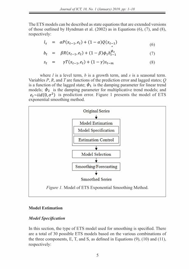
The ETS models can be described as state equations that are extended versions of those outlined by
Hyndman et al. (2002) as in Equations (6), (7), and (8), respectively:
𝑙𝑠 = 𝛼𝑃(𝑥𝑡−1, 𝑒𝑡) + (1 − 𝛼)𝑄(𝑥𝑡−1)𝑏𝑡 = 𝛽𝑅(𝑥𝑡−1, 𝑒𝑡) + (1 − 𝛽)𝜙1𝑏𝑡−1
𝜙2
𝑠𝑡 = 𝛾𝑇(𝑥𝑡−1, 𝑒𝑡) + (1 − 𝛾)𝑠𝑡−�
(6) (7) (8)
where l is a level term, b is a growth term, and s is a seasonal term. Variables P, R, and T are
functions of the prediction error and lagged states; Q is a function of the lagged state; 𝜙1 is the
damping parameter for linear trend models; 𝜙2 is the damping parameter for multiplicative trend
models; and 𝑒𝑡~𝑖𝑖𝑑(0,𝜎2) is prediction error. Figure 1 presents the model of ETS exponential
smoothing method.
5
Journal of ICT, 18, No. 1 (January) 2019, pp: 1–18
The ETS models can be described as state equations that are extended versions of those outlined by Hyndman et al. (2002) as in Equations (6), (7), and (8), respectively:
(6)
(7)
(8)
where l is a level term, b is a growth term, and s is a seasonal term. Variables P, R, and T are functions of the prediction error and lagged states; Q is a function of the lagged state; is the damping parameter for linear trend models; is the damping parameter for multiplicative trend models; and is prediction error. Figure 1 presents the model of ETS exponential smoothing method.
Figure 1. Model of ETS Exponential Smoothing Method.
Model Estimation
Model Specification
In this section, the type of ETS model used for smoothing is specified. There are a total of 30 possible ETS models based on the various combinations of the three components, E, T, and S, as defined in Equations (9), (10) and (11), respectively:
4
The forecasts are computed by:
𝑥�𝑡+𝑖 = (𝑎(𝑇) + 𝑏(𝑇)𝑖)𝑐𝑇+𝑖−𝑠 (5)
where the seasonal factors are used from the last s estimates.
ETS EXPONENTIAL SMOOTHING
This framework defines an extended class of exponential smoothing methods and offers a theoretical
foundation for analysis of these models using state-space based likelihood calculations. Support for
model selection and calculation of forecast standard errors are also included. The standard exponential
smoothing models discussed in the previous section, such as HWMS, are encompassed by this ETS
framework.
In the ETS exponential smoothing method, the time series may be decomposed into three
components, namely the error (E) that is the irregular unpredictable component of the series, the trend
(T) that characterizes the long-term movement of the time series, and the season (S) that corresponds
to a pattern with known periodicity.
The ETS models can be described as state equations that are extended versions of those outlined by
Hyndman et al. (2002) as in Equations (6), (7), and (8), respectively:
𝑙𝑠 = 𝛼𝑃(𝑥𝑡−1, 𝑒𝑡) + (1 − 𝛼)𝑄(𝑥𝑡−1)𝑏𝑡 = 𝛽𝑅(𝑥𝑡−1, 𝑒𝑡) + (1 − 𝛽)𝜙1𝑏𝑡−1
𝜙2
𝑠𝑡 = 𝛾𝑇(𝑥𝑡−1, 𝑒𝑡) + (1 − 𝛾)𝑠𝑡−�
(6) (7) (8)
where l is a level term, b is a growth term, and s is a seasonal term. Variables P, R, and T are
functions of the prediction error and lagged states; Q is a function of the lagged state; 𝜙1 is the
damping parameter for linear trend models; 𝜙2 is the damping parameter for multiplicative trend
models; and 𝑒𝑡~𝑖𝑖𝑑(0,𝜎2) is prediction error. Figure 1 presents the model of ETS exponential
smoothing method.
Journal of ICT, 18, No. 1 (January) 2019, pp: 1–18
6
E {A, M} (9)
T {N, A, M, AD, MD} (10)
S {N, A, M} (11)
where N = none, A = additive, M = multiplicative, AD = additive dampened, and MD = multiplicative dampened.
Estimation Control
According to the chosen ETS model specification, the corresponding unknown parameters and the initial states x0 may be estimated using either the maximum likelihood or average mean square error minimization (AMSE) methods.
The Gaussian log likelihood for ETS specifications can be written in terms of the prediction errors, as in Equation (12):
(12)
The parameters and initial states are achieved by maximizing the likelihood in Equation (12) with respect to and using the Broyden, Fletcher, Goldfarb, and Shanno (BFGS) algorithm (Fletcher, 1987).
The average mean square error (AMSE) of the h-step forecasts is expressed as in Equation (13):
(13)
The parameters and initial states that minimize the AMSE using BFGS are then achieved.
Model Selection
In this step, the model can be selected based on either the comparison of a likelihood-based information criterion across the models to decide which one more closely fits the data or the forecast error, i.e., an out-of-sample AMSE to decide which one has a more accurate forecast result.
The likelihood-based information criteria include Akaike information criterion (AIC), Schwarz information criterion (BIC), or the Hannan-Quinn criterion (HQ), as expressed in Equations (14), (15), and (16), respectively:
5
Figure 1. Model of ETS Exponential Smoothing Method.
(1) Model Estimation
Model Specification
In this section, the type of ETS model used for smoothing is specified. There are a total of 30 possible
ETS models based on the various combinations of the three components, E, T, and S, as defined in
Equations (9), (10) and (11), respectively:
E {A, M} (9)
T {N, A, M, AD, MD} (10)
S {N, A, M} (11)
where N = none, A = additive, M = multiplicative, AD = additive dampened, and MD = multiplicative
dampened.
Estimation Control
According to the chosen ETS model specification, the corresponding unknown parameters 𝜃 =(𝛼,𝛽, 𝛾,𝜙), and the initial states x0 may be estimated using either the maximum likelihood or average
mean square error minimization (AMSE) methods.
Original Series
Model Estimation Model Specification
Estimation Control
Model Selection
Smoothing/Forecasting
Smoothed Series
6
The Gaussian log likelihood for ETS specifications can be written in terms of the prediction errors, as
in Equation (12):
𝑙𝑜𝑔 𝐿(𝜃, 𝑥0,𝜎2|𝑦) = − 2𝑇 𝑙𝑜𝑔(2𝜋𝜎2) − 1
2∑𝑒𝑡2𝜎2
�𝑡−1 . (12)
The parameters and initial states are achieved by maximizing the likelihood in Equation (12) with
respect to 𝜃, 𝑥0, and 𝜎2 using the Broyden, Fletcher, Goldfarb, and Shanno (BFGS) algorithm
(Fletcher, 1987).
The average mean square error (AMSE) of the h-step forecasts is expressed as in Equation (13):
𝐴𝑀𝑆𝐸 = 1𝑇 ∑ �1ℎ ∑ 𝑒𝑡+�|𝑡
2ℎ�=1 �ℎ
�=1 . (13)
The parameters and initial states that minimize the AMSE using BFGS are then achieved.
(2) Model Selection
In this step, the model can be selected based on either the comparison of a likelihood-based
information criterion across the models to decide which one more closely fits the data or the forecast
error, i.e., an out-of-sample AMSE to decide which one has a more accurate forecast result.
The likelihood-based information criteria include Akaike information criterion (AIC), Schwarz
information criterion (BIC), or the Hannan-Quinn criterion (HQ), as expressed in Equations (14),
(15), and (16), respectively:
𝐴𝐼𝐶 = −2 𝑙𝑜𝑔 𝐿�𝜃�, 𝑥�0� + 2𝑝𝐵𝐼𝐶 = −2 𝑙𝑜𝑔 𝐿�𝜃�,𝑥�0� + 𝑙𝑜𝑔(𝑇)𝑝𝐻𝑄 = −2 𝑙𝑜𝑔 𝐿�𝜃�, 𝑥�0� + 2 𝑙𝑜𝑔(𝑙𝑜𝑔 𝑇)𝑝
(14)
(15)
(16)
where �𝜃�,𝑥�0� are the maximized values and p is the number of parameters in 𝜃� plus the number of the
estimated initial states in 𝑥�0. The chosen model is the one with the minimum value of AIC (BIC, or
HQ).
The out-of-sample AMSE is given in Equation (17):
𝐴𝑀𝑆𝐸 = 1𝑇∗ ∑ �1ℎ ∑ 𝑒𝑡+�|𝑡
2ℎ�=1 �𝑇+𝑇∗
𝑡=𝑇+1 . (17)
(3) Smoothing/Forecasting
Using the chosen ETS model with estimated parameters, the in-sample smoothed series can be
achieved by the one-step-ahead forecast function, ℎ(𝑥𝑡−1,𝜃). Based on the smoothing model and the 6
The Gaussian log likelihood for ETS specifications can be written in terms of the prediction errors, as
in Equation (12):
𝑙𝑜𝑔 𝐿(𝜃, 𝑥0,𝜎2|𝑦) = − 2𝑇 𝑙𝑜𝑔(2𝜋𝜎2) − 1
2∑𝑒𝑡2𝜎2
�𝑡−1 . (12)
The parameters and initial states are achieved by maximizing the likelihood in Equation (12) with
respect to 𝜃, 𝑥0, and 𝜎2 using the Broyden, Fletcher, Goldfarb, and Shanno (BFGS) algorithm
(Fletcher, 1987).
The average mean square error (AMSE) of the h-step forecasts is expressed as in Equation (13):
𝐴𝑀𝑆𝐸 = 1𝑇 ∑ �1ℎ ∑ 𝑒𝑡+�|𝑡
2ℎ�=1 �ℎ
�=1 . (13)
The parameters and initial states that minimize the AMSE using BFGS are then achieved.
(2) Model Selection
In this step, the model can be selected based on either the comparison of a likelihood-based
information criterion across the models to decide which one more closely fits the data or the forecast
error, i.e., an out-of-sample AMSE to decide which one has a more accurate forecast result.
The likelihood-based information criteria include Akaike information criterion (AIC), Schwarz
information criterion (BIC), or the Hannan-Quinn criterion (HQ), as expressed in Equations (14),
(15), and (16), respectively:
𝐴𝐼𝐶 = −2 𝑙𝑜𝑔 𝐿�𝜃�, 𝑥�0� + 2𝑝𝐵𝐼𝐶 = −2 𝑙𝑜𝑔 𝐿�𝜃�,𝑥�0� + 𝑙𝑜𝑔(𝑇)𝑝𝐻𝑄 = −2 𝑙𝑜𝑔 𝐿�𝜃�, 𝑥�0� + 2 𝑙𝑜𝑔(𝑙𝑜𝑔 𝑇)𝑝
(14)
(15)
(16)
where �𝜃�,𝑥�0� are the maximized values and p is the number of parameters in 𝜃� plus the number of the
estimated initial states in 𝑥�0. The chosen model is the one with the minimum value of AIC (BIC, or
HQ).
The out-of-sample AMSE is given in Equation (17):
𝐴𝑀𝑆𝐸 = 1𝑇∗ ∑ �1ℎ ∑ 𝑒𝑡+�|𝑡
2ℎ�=1 �𝑇+𝑇∗
𝑡=𝑇+1 . (17)
(3) Smoothing/Forecasting
Using the chosen ETS model with estimated parameters, the in-sample smoothed series can be
achieved by the one-step-ahead forecast function, ℎ(𝑥𝑡−1,𝜃). Based on the smoothing model and the
7
Journal of ICT, 18, No. 1 (January) 2019, pp: 1–18
(14)
(15)
(16)
where are the maximized values and p is the number of parameters in plus the number of the estimated initial states in . The chosen model is the one with the minimum value of AIC (BIC, or HQ).
The out-of-sample AMSE is given in Equation (17):
(17)
Smoothing/Forecasting
Using the chosen ETS model with estimated parameters, the in-sample smoothed series can be achieved by the one-step-ahead forecast function, Based on the smoothing model and the estimated parameters, as well as the in-sample data, the out-of-sample forecasted values can be obtained by implementing the dynamic forecast of the series.
EXPERIMENTAL METHODOLOGY AND RESULT
The real traffic from commercial cellular networks was collected and included voice in Erlang and data in Mbps. The first trace is 31-day hourly voice traffic collected during the New Year period from MSCID of MSC_Hanoi1. The traffic data ranged from 00:00 December 9th, 2015 until 23:00 January 8th, 2016 and included 744 observations. The second trace is the daily voice traffic and included 236 3G traffic values that ranged from March 9th until October 30th, 2014, collected from 110 siteBs in the CauGiay district area in Hanoi. The third trace is the 3G data collected from 600 cells located within the HoanKiem district in Hanoi. The 443-value daily data traffic series ranged from September 12th, 2014 to November 28th, 2015. Exponential smoothing methods were applied to forecast these three traces that are distinguished from each other by traffic type, namely voice vs. data and hourly vs. daily. The simple exponential smoothing methods included single, double, and Holt-Winters and were used to implement the forecasts for the three traffic traces. Then, the achieved models that gave the best results were chosen to make comparisons with the best choices by the
6
The Gaussian log likelihood for ETS specifications can be written in terms of the prediction errors, as
in Equation (12):
𝑙𝑜𝑔 𝐿(𝜃, 𝑥0,𝜎2|𝑦) = − 2𝑇 𝑙𝑜𝑔(2𝜋𝜎2) − 1
2∑𝑒𝑡2𝜎2
�𝑡−1 . (12)
The parameters and initial states are achieved by maximizing the likelihood in Equation (12) with
respect to 𝜃, 𝑥0, and 𝜎2 using the Broyden, Fletcher, Goldfarb, and Shanno (BFGS) algorithm
(Fletcher, 1987).
The average mean square error (AMSE) of the h-step forecasts is expressed as in Equation (13):
𝐴𝑀𝑆𝐸 = 1𝑇 ∑ �1ℎ ∑ 𝑒𝑡+�|𝑡
2ℎ�=1 �ℎ
�=1 . (13)
The parameters and initial states that minimize the AMSE using BFGS are then achieved.
(2) Model Selection
In this step, the model can be selected based on either the comparison of a likelihood-based
information criterion across the models to decide which one more closely fits the data or the forecast
error, i.e., an out-of-sample AMSE to decide which one has a more accurate forecast result.
The likelihood-based information criteria include Akaike information criterion (AIC), Schwarz
information criterion (BIC), or the Hannan-Quinn criterion (HQ), as expressed in Equations (14),
(15), and (16), respectively:
𝐴𝐼𝐶 = −2 𝑙𝑜𝑔 𝐿�𝜃�, 𝑥�0� + 2𝑝𝐵𝐼𝐶 = −2 𝑙𝑜𝑔 𝐿�𝜃�,𝑥�0� + 𝑙𝑜𝑔(𝑇)𝑝𝐻𝑄 = −2 𝑙𝑜𝑔 𝐿�𝜃�, 𝑥�0� + 2 𝑙𝑜𝑔(𝑙𝑜𝑔 𝑇)𝑝
(14)
(15)
(16)
where �𝜃�,𝑥�0� are the maximized values and p is the number of parameters in 𝜃� plus the number of the
estimated initial states in 𝑥�0. The chosen model is the one with the minimum value of AIC (BIC, or
HQ).
The out-of-sample AMSE is given in Equation (17):
𝐴𝑀𝑆𝐸 = 1𝑇∗ ∑ �1ℎ ∑ 𝑒𝑡+�|𝑡
2ℎ�=1 �𝑇+𝑇∗
𝑡=𝑇+1 . (17)
(3) Smoothing/Forecasting
Using the chosen ETS model with estimated parameters, the in-sample smoothed series can be
achieved by the one-step-ahead forecast function, ℎ(𝑥𝑡−1,𝜃). Based on the smoothing model and the
6
The Gaussian log likelihood for ETS specifications can be written in terms of the prediction errors, as
in Equation (12):
𝑙𝑜𝑔 𝐿(𝜃, 𝑥0,𝜎2|𝑦) = − 2𝑇 𝑙𝑜𝑔(2𝜋𝜎2) − 1
2∑𝑒𝑡2𝜎2
�𝑡−1 . (12)
The parameters and initial states are achieved by maximizing the likelihood in Equation (12) with
respect to 𝜃, 𝑥0, and 𝜎2 using the Broyden, Fletcher, Goldfarb, and Shanno (BFGS) algorithm
(Fletcher, 1987).
The average mean square error (AMSE) of the h-step forecasts is expressed as in Equation (13):
𝐴𝑀𝑆𝐸 = 1𝑇 ∑ �1ℎ ∑ 𝑒𝑡+�|𝑡
2ℎ�=1 �ℎ
�=1 . (13)
The parameters and initial states that minimize the AMSE using BFGS are then achieved.
(2) Model Selection
In this step, the model can be selected based on either the comparison of a likelihood-based
information criterion across the models to decide which one more closely fits the data or the forecast
error, i.e., an out-of-sample AMSE to decide which one has a more accurate forecast result.
The likelihood-based information criteria include Akaike information criterion (AIC), Schwarz
information criterion (BIC), or the Hannan-Quinn criterion (HQ), as expressed in Equations (14),
(15), and (16), respectively:
𝐴𝐼𝐶 = −2 𝑙𝑜𝑔 𝐿�𝜃�, 𝑥�0� + 2𝑝𝐵𝐼𝐶 = −2 𝑙𝑜𝑔 𝐿�𝜃�,𝑥�0� + 𝑙𝑜𝑔(𝑇)𝑝𝐻𝑄 = −2 𝑙𝑜𝑔 𝐿�𝜃�, 𝑥�0� + 2 𝑙𝑜𝑔(𝑙𝑜𝑔 𝑇)𝑝
(14)
(15)
(16)
where �𝜃�,𝑥�0� are the maximized values and p is the number of parameters in 𝜃� plus the number of the
estimated initial states in 𝑥�0. The chosen model is the one with the minimum value of AIC (BIC, or
HQ).
The out-of-sample AMSE is given in Equation (17):
𝐴𝑀𝑆𝐸 = 1𝑇∗ ∑ �1ℎ ∑ 𝑒𝑡+�|𝑡
2ℎ�=1 �𝑇+𝑇∗
𝑡=𝑇+1 . (17)
(3) Smoothing/Forecasting
Using the chosen ETS model with estimated parameters, the in-sample smoothed series can be
achieved by the one-step-ahead forecast function, ℎ(𝑥𝑡−1,𝜃). Based on the smoothing model and the 6
The Gaussian log likelihood for ETS specifications can be written in terms of the prediction errors, as
in Equation (12):
𝑙𝑜𝑔 𝐿(𝜃, 𝑥0,𝜎2|𝑦) = − 2𝑇 𝑙𝑜𝑔(2𝜋𝜎2) − 1
2∑𝑒𝑡2𝜎2
�𝑡−1 . (12)
The parameters and initial states are achieved by maximizing the likelihood in Equation (12) with
respect to 𝜃, 𝑥0, and 𝜎2 using the Broyden, Fletcher, Goldfarb, and Shanno (BFGS) algorithm
(Fletcher, 1987).
The average mean square error (AMSE) of the h-step forecasts is expressed as in Equation (13):
𝐴𝑀𝑆𝐸 = 1𝑇 ∑ �1ℎ ∑ 𝑒𝑡+�|𝑡
2ℎ�=1 �ℎ
�=1 . (13)
The parameters and initial states that minimize the AMSE using BFGS are then achieved.
(2) Model Selection
In this step, the model can be selected based on either the comparison of a likelihood-based
information criterion across the models to decide which one more closely fits the data or the forecast
error, i.e., an out-of-sample AMSE to decide which one has a more accurate forecast result.
The likelihood-based information criteria include Akaike information criterion (AIC), Schwarz
information criterion (BIC), or the Hannan-Quinn criterion (HQ), as expressed in Equations (14),
(15), and (16), respectively:
𝐴𝐼𝐶 = −2 𝑙𝑜𝑔 𝐿�𝜃�, 𝑥�0� + 2𝑝𝐵𝐼𝐶 = −2 𝑙𝑜𝑔 𝐿�𝜃�,𝑥�0� + 𝑙𝑜𝑔(𝑇)𝑝𝐻𝑄 = −2 𝑙𝑜𝑔 𝐿�𝜃�, 𝑥�0� + 2 𝑙𝑜𝑔(𝑙𝑜𝑔 𝑇)𝑝
(14)
(15)
(16)
where �𝜃�,𝑥�0� are the maximized values and p is the number of parameters in 𝜃� plus the number of the
estimated initial states in 𝑥�0. The chosen model is the one with the minimum value of AIC (BIC, or
HQ).
The out-of-sample AMSE is given in Equation (17):
𝐴𝑀𝑆𝐸 = 1𝑇∗ ∑ �1ℎ ∑ 𝑒𝑡+�|𝑡
2ℎ�=1 �𝑇+𝑇∗
𝑡=𝑇+1 . (17)
(3) Smoothing/Forecasting
Using the chosen ETS model with estimated parameters, the in-sample smoothed series can be
achieved by the one-step-ahead forecast function, ℎ(𝑥𝑡−1,𝜃). Based on the smoothing model and the
6
The Gaussian log likelihood for ETS specifications can be written in terms of the prediction errors, as
in Equation (12):
𝑙𝑜𝑔 𝐿(𝜃, 𝑥0,𝜎2|𝑦) = − 2𝑇 𝑙𝑜𝑔(2𝜋𝜎2) − 1
2∑𝑒𝑡2𝜎2
�𝑡−1 . (12)
The parameters and initial states are achieved by maximizing the likelihood in Equation (12) with
respect to 𝜃, 𝑥0, and 𝜎2 using the Broyden, Fletcher, Goldfarb, and Shanno (BFGS) algorithm
(Fletcher, 1987).
The average mean square error (AMSE) of the h-step forecasts is expressed as in Equation (13):
𝐴𝑀𝑆𝐸 = 1𝑇 ∑ �1ℎ ∑ 𝑒𝑡+�|𝑡
2ℎ�=1 �ℎ
�=1 . (13)
The parameters and initial states that minimize the AMSE using BFGS are then achieved.
(2) Model Selection
In this step, the model can be selected based on either the comparison of a likelihood-based
information criterion across the models to decide which one more closely fits the data or the forecast
error, i.e., an out-of-sample AMSE to decide which one has a more accurate forecast result.
The likelihood-based information criteria include Akaike information criterion (AIC), Schwarz
information criterion (BIC), or the Hannan-Quinn criterion (HQ), as expressed in Equations (14),
(15), and (16), respectively:
𝐴𝐼𝐶 = −2 𝑙𝑜𝑔 𝐿�𝜃�, 𝑥�0� + 2𝑝𝐵𝐼𝐶 = −2 𝑙𝑜𝑔 𝐿�𝜃�,𝑥�0� + 𝑙𝑜𝑔(𝑇)𝑝𝐻𝑄 = −2 𝑙𝑜𝑔 𝐿�𝜃�, 𝑥�0� + 2 𝑙𝑜𝑔(𝑙𝑜𝑔 𝑇)𝑝
(14)
(15)
(16)
where �𝜃�,𝑥�0� are the maximized values and p is the number of parameters in 𝜃� plus the number of the
estimated initial states in 𝑥�0. The chosen model is the one with the minimum value of AIC (BIC, or
HQ).
The out-of-sample AMSE is given in Equation (17):
𝐴𝑀𝑆𝐸 = 1𝑇∗ ∑ �1ℎ ∑ 𝑒𝑡+�|𝑡
2ℎ�=1 �𝑇+𝑇∗
𝑡=𝑇+1 . (17)
(3) Smoothing/Forecasting
Using the chosen ETS model with estimated parameters, the in-sample smoothed series can be
achieved by the one-step-ahead forecast function, ℎ(𝑥𝑡−1,𝜃). Based on the smoothing model and the
6
The likelihood-based information criteria include Akaike information criterion (AIC), Schwarz
information criterion (BIC), or the Hannan-Quinn criterion (HQ), as expressed in Equations (14),
(15), and (16), respectively:
𝐴𝐼𝐶 = −2 𝑙𝑜𝑔𝐿�𝜃�,𝑥�0�+ 2𝑝𝐵𝐼𝐶 = −2 𝑙𝑜𝑔𝐿�𝜃�, 𝑥�0�+ 𝑙𝑜𝑔(𝑇)𝑝𝐻𝑄 = −2 𝑙𝑜𝑔 𝐿�𝜃�,𝑥�0�+ 2 𝑙𝑜𝑔(𝑙𝑜𝑔𝑇)𝑝
(14)
(15)
(16)
where �𝜃�,𝑥�0� are the maximized values and p is the number of parameters in 𝜃� plus the number of the
estimated initial states in 𝑥�0. The chosen model is the one with the minimum value of AIC (BIC, or
HQ).
The out-of-sample AMSE is given in Equation (17):
𝐴𝑀𝑆𝐸= 1𝑇∗∑ �1
ℎ∑ 𝑒𝑡+𝑘|𝑡
2ℎ𝑘=1 �𝑇+𝑇∗
𝑡=𝑇+1 . (17)
(3) Smoothing/Forecasting
Using the chosen ETS model with estimated parameters, the in-sample smoothed series can be
achieved by the one-step-ahead forecast function, ℎ(𝑥𝑡−1,𝜃). Based on the smoothing model and the
estimated parameters, as well as the in-sample data, the out-of-sample forecasted values can be
obtained by implementing the dynamic forecast of the series.
EXPERIMENTAL METHODOLOGY AND RESULTS
The real traffic from commercial cellular networks was collected and included voice in Erlang and
data in Mbps. The first trace is 31-day hourly voice traffic collected during the New Year period from
MSCID of MSC_Hanoi1. The traffic data ranged from 00:00 December 9th, 2015 until 23:00 January
8th, 2016 and included 744 observations. The second trace is the daily voice traffic and included 236
3G traffic values that ranged from March 9th until October 30th, 2014, collected from 110 siteBs in
the CauGiay district area in Hanoi. The third trace is the 3G data collected from 600 cells located
within the HoanKiem district in Hanoi. The 443-value daily data traffic series ranged from September
12th, 2014 to November 28th, 2015.
Exponential smoothing methods were applied to forecast these three traces that are distinguished from
each other by traffic type, namely voice vs. data and hourly vs. daily. The simple exponential
smoothing methods included single, double , and Holt-Winters and were used to implement the
forecasts for the three traffic traces. Then, the achieved models that gave the best results were chosen
to make comparisons with the best choices by the ETS exponential smoothing framework in terms of
estimation information, in-sample forecast, and out-of-sample forecast.
6
The likelihood-based information criteria include Akaike information criterion (AIC), Schwarz
information criterion (BIC), or the Hannan-Quinn criterion (HQ), as expressed in Equations (14),
(15), and (16), respectively:
𝐴𝐼𝐶 = −2 𝑙𝑜𝑔𝐿�𝜃�,𝑥�0�+ 2𝑝𝐵𝐼𝐶 = −2 𝑙𝑜𝑔𝐿�𝜃�, 𝑥�0�+ 𝑙𝑜𝑔(𝑇)𝑝𝐻𝑄 = −2 𝑙𝑜𝑔 𝐿�𝜃�,𝑥�0�+ 2 𝑙𝑜𝑔(𝑙𝑜𝑔𝑇)𝑝
(14)
(15)
(16)
where �𝜃�,𝑥�0� are the maximized values and p is the number of parameters in 𝜃� plus the number of the
estimated initial states in 𝑥�0. The chosen model is the one with the minimum value of AIC (BIC, or
HQ).
The out-of-sample AMSE is given in Equation (17):
𝐴𝑀𝑆𝐸= 1𝑇∗∑ �1
ℎ∑ 𝑒𝑡+𝑘|𝑡
2ℎ𝑘=1 �𝑇+𝑇∗
𝑡=𝑇+1 . (17)
(3) Smoothing/Forecasting
Using the chosen ETS model with estimated parameters, the in-sample smoothed series can be
achieved by the one-step-ahead forecast function, ℎ(𝑥𝑡−1,𝜃). Based on the smoothing model and the
estimated parameters, as well as the in-sample data, the out-of-sample forecasted values can be
obtained by implementing the dynamic forecast of the series.
EXPERIMENTAL METHODOLOGY AND RESULTS
The real traffic from commercial cellular networks was collected and included voice in Erlang and
data in Mbps. The first trace is 31-day hourly voice traffic collected during the New Year period from
MSCID of MSC_Hanoi1. The traffic data ranged from 00:00 December 9th, 2015 until 23:00 January
8th, 2016 and included 744 observations. The second trace is the daily voice traffic and included 236
3G traffic values that ranged from March 9th until October 30th, 2014, collected from 110 siteBs in
the CauGiay district area in Hanoi. The third trace is the 3G data collected from 600 cells located
within the HoanKiem district in Hanoi. The 443-value daily data traffic series ranged from September
12th, 2014 to November 28th, 2015.
Exponential smoothing methods were applied to forecast these three traces that are distinguished from
each other by traffic type, namely voice vs. data and hourly vs. daily. The simple exponential
smoothing methods included single, double , and Holt-Winters and were used to implement the
forecasts for the three traffic traces. Then, the achieved models that gave the best results were chosen
to make comparisons with the best choices by the ETS exponential smoothing framework in terms of
estimation information, in-sample forecast, and out-of-sample forecast. 6
The likelihood-based information criteria include Akaike information criterion (AIC), Schwarz
information criterion (BIC), or the Hannan-Quinn criterion (HQ), as expressed in Equations (14),
(15), and (16), respectively:
𝐴𝐼𝐶 = −2 𝑙𝑜𝑔𝐿�𝜃�,𝑥�0�+ 2𝑝𝐵𝐼𝐶 = −2 𝑙𝑜𝑔𝐿�𝜃�, 𝑥�0�+ 𝑙𝑜𝑔(𝑇)𝑝𝐻𝑄 = −2 𝑙𝑜𝑔 𝐿�𝜃�,𝑥�0�+ 2 𝑙𝑜𝑔(𝑙𝑜𝑔𝑇)𝑝
(14)
(15)
(16)
where �𝜃�,𝑥�0� are the maximized values and p is the number of parameters in 𝜃� plus the number of the
estimated initial states in 𝑥�0. The chosen model is the one with the minimum value of AIC (BIC, or
HQ).
The out-of-sample AMSE is given in Equation (17):
𝐴𝑀𝑆𝐸= 1𝑇∗∑ �1
ℎ∑ 𝑒𝑡+𝑘|𝑡
2ℎ𝑘=1 �𝑇+𝑇∗
𝑡=𝑇+1 . (17)
(3) Smoothing/Forecasting
Using the chosen ETS model with estimated parameters, the in-sample smoothed series can be
achieved by the one-step-ahead forecast function, ℎ(𝑥𝑡−1,𝜃). Based on the smoothing model and the
estimated parameters, as well as the in-sample data, the out-of-sample forecasted values can be
obtained by implementing the dynamic forecast of the series.
EXPERIMENTAL METHODOLOGY AND RESULTS
The real traffic from commercial cellular networks was collected and included voice in Erlang and
data in Mbps. The first trace is 31-day hourly voice traffic collected during the New Year period from
MSCID of MSC_Hanoi1. The traffic data ranged from 00:00 December 9th, 2015 until 23:00 January
8th, 2016 and included 744 observations. The second trace is the daily voice traffic and included 236
3G traffic values that ranged from March 9th until October 30th, 2014, collected from 110 siteBs in
the CauGiay district area in Hanoi. The third trace is the 3G data collected from 600 cells located
within the HoanKiem district in Hanoi. The 443-value daily data traffic series ranged from September
12th, 2014 to November 28th, 2015.
Exponential smoothing methods were applied to forecast these three traces that are distinguished from
each other by traffic type, namely voice vs. data and hourly vs. daily. The simple exponential
smoothing methods included single, double , and Holt-Winters and were used to implement the
forecasts for the three traffic traces. Then, the achieved models that gave the best results were chosen
to make comparisons with the best choices by the ETS exponential smoothing framework in terms of
estimation information, in-sample forecast, and out-of-sample forecast.
Journal of ICT, 18, No. 1 (January) 2019, pp: 1–18
8
ETS exponential smoothing framework in terms of estimation information, in-sample forecast, and out-of-sample forecast.
Hourly Voice Traffic
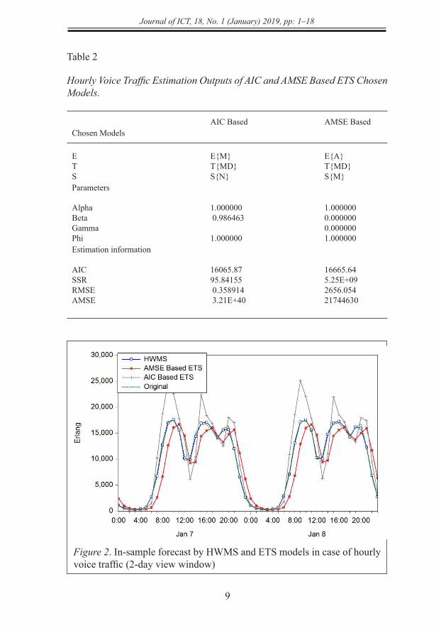
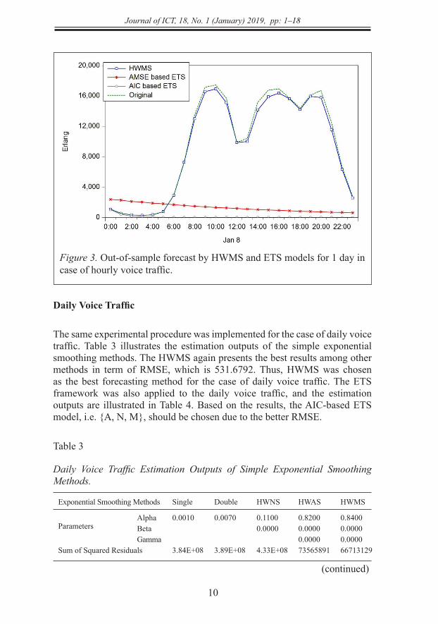
The simple exponential smoothing methods were applied to hourly voice traffic. The estimation outputs are shown in Table 1, where HWMS presents the best results in terms of the 426.5057 RMSE. Thus, the HWMS was chosen as the best forecasting method in the case of hourly voice traffic. In contrast, the ETS framework was also applied to this hourly voice traffic, and the estimation outputs are listed in Table 2. The numerical results indicate that this framework is not suitable for the hourly data series when both AIC-based and AMSE-based models yield abnormal RMSE values. To confirm this judgment, we further implement the in-sample and out-of-sample forecast tests for these two models and compare the results with those obtained using HWMS. The results are shown in Figures 2 and 3 which display that the HWMS out-of-sample forecasted data is very close to the original data, so we can figure out that HWMS outperforms the two ETS models in modeling and forecasting hourly cellular voice traffic.
Table 1
Hourly Voice Traffic Estimation Outputs of Simple Exponential Smoothing Methods.
Exponential Smoothing Methods
Single
Double
HWNS
HWAS
HWMS
Parameters
Alpha 0.9990 0.9990 1.0000 1.0000 1.0000
Beta 1.0000 0.0000 0.0000
Gamma 0.0000 0.0000
Sum of Squared Residuals 5.36E+09 4.15E+09 4.05E+09 2.36E+08 1.35E+08
Root Mean Squared Error 2684.505 2363.002 2334.268 563.0144 426.5057
End of Period Levels
Mean 2797.097 2793.238 2793.240 9059.919 10147.16
Trend -3854.95 -3850.91 1.419014 1.419014
9
Journal of ICT, 18, No. 1 (January) 2019, pp: 1–18
Table 2
Hourly Voice Traffic Estimation Outputs of AIC and AMSE Based ETS Chosen Models.
AIC Based AMSE BasedChosen Models
ETS
E{M}T{MD}S{N}
E{A}T{MD}S{M}
Parameters
AlphaBetaGammaPhi
1.000000 0.986463
1.000000
1.0000000.0000000.0000001.000000
Estimation information
AICSSRRMSEAMSE
16065.8795.84155 0.358914 3.21E+40
16665.645.25E+092656.05421744630
Figure 2. In-sample forecast by HWMS and ETS models in case of hourly voice traffic (2-day view window)
8
Figure 2. In-sample forecast by HWMS and ETS models in case of hourly voice traffic (2-day view window)
Figure 3. Out-of-sample forecast by HWMS and ETS models for 1 day in case of hourly voice traffic.
(2) Daily Voice Traffic
The same experimental procedure was implemented for the case of daily voice traffic. Table 3
illustrates the estimation outputs of the simple exponential smoothing methods. The HWMS again
presents the best results among other methods in term of RMSE, which is 531.6792. Thus, HWMS
was chosen as the best forecasting method for the case of daily voice traffic. The ETS framework was
Journal of ICT, 18, No. 1 (January) 2019, pp: 1–18
10
Figure 3. Out-of-sample forecast by HWMS and ETS models for 1 day in case of hourly voice traffic.
Daily Voice Traffic
The same experimental procedure was implemented for the case of daily voice traffic. Table 3 illustrates the estimation outputs of the simple exponential smoothing methods. The HWMS again presents the best results among other methods in term of RMSE, which is 531.6792. Thus, HWMS was chosen as the best forecasting method for the case of daily voice traffic. The ETS framework was also applied to the daily voice traffic, and the estimation outputs are illustrated in Table 4. Based on the results, the AIC-based ETS model, i.e. {A, N, M}, should be chosen due to the better RMSE.
Table 3
Daily Voice Traffic Estimation Outputs of Simple Exponential Smoothing Methods.
Exponential Smoothing Methods Single Double HWNS HWAS HWMS
ParametersAlpha 0.0010 0.0070 0.1100 0.8200 0.8400Beta 0.0000 0.0000 0.0000Gamma 0.0000 0.0000
Sum of Squared Residuals 3.84E+08 3.89E+08 4.33E+08 73565891 66713129
(continued)
8
Figure 2. In-sample forecast by HWMS and ETS models in case of hourly voice traffic (2-day view window)
Figure 3. Out-of-sample forecast by HWMS and ETS models for 1 day in case of hourly voice traffic.
(2) Daily Voice Traffic
The same experimental procedure was implemented for the case of daily voice traffic. Table 3
illustrates the estimation outputs of the simple exponential smoothing methods. The HWMS again
presents the best results among other methods in term of RMSE, which is 531.6792. Thus, HWMS
was chosen as the best forecasting method for the case of daily voice traffic. The ETS framework was
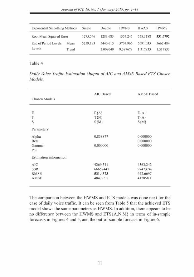
11
Journal of ICT, 18, No. 1 (January) 2019, pp: 1–18
Exponential Smoothing Methods Single Double HWNS HWAS HWMS
Root Mean Squared Error 1275.546 1283.683 1354.245 558.3188 531.6792
End of Period LevelsLevels
Mean 5259.193 5440.615 5707.966 5691.035 5662.484
Trend 2.008049 9.387678 1.317833 1.317833
Table 4
Daily Voice Traffic Estimation Output of AIC and AMSE Based ETS Chosen Models.
AIC Based AMSE Based
Chosen Models
ETS
E{A}T{N}S{M}
E{A}T{A}S{M}
Parameters
AlphaBetaGammaPhi
0.838877
0.000000
0.0000000.0000000.000000
Estimation information
AICSSRRMSEAMSE
4269.54166652447531.4373484775.5
4363.24297473742642.6697412858.1
The comparison between the HWMS and ETS models was done next for the case of daily voice traffic. It can be seen from Table 5 that the achieved ETS model shows the same parameters as HWMS. In addition, there appears to be no difference between the HWMS and ETS{A,N,M} in terms of in-sample forecasts in Figures 4 and 5, and the out-of-sample forecast in Figure 6.
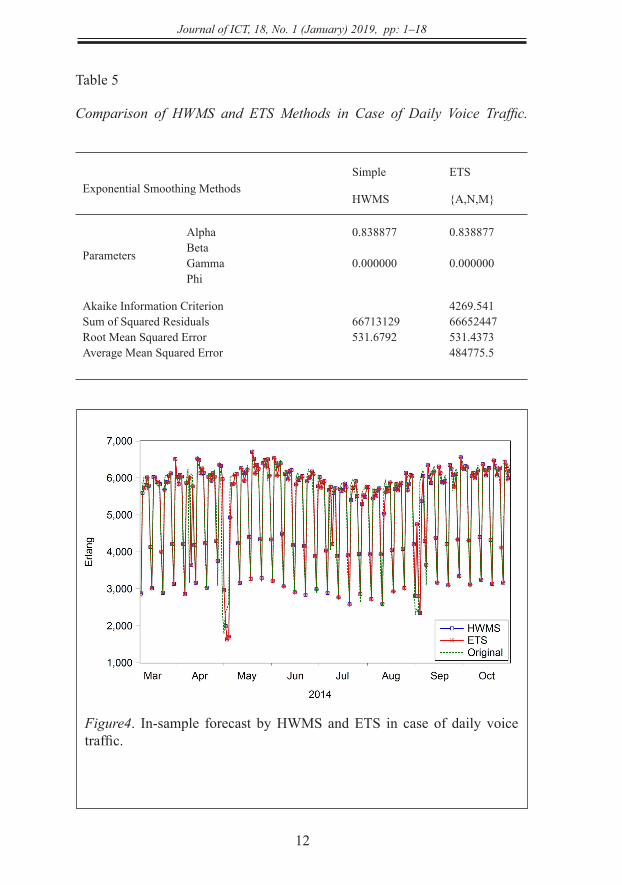
Journal of ICT, 18, No. 1 (January) 2019, pp: 1–18
12
Table 5
Comparison of HWMS and ETS Methods in Case of Daily Voice Traffic.
Exponential Smoothing MethodsSimple ETS
HWMS {A,N,M}
Parameters
AlphaBetaGammaPhi
0.838877
0.000000
0.838877
0.000000
Akaike Information CriterionSum of Squared ResidualsRoot Mean Squared ErrorAverage Mean Squared Error
66713129531.6792
4269.54166652447531.4373484775.5
Figure4. In-sample forecast by HWMS and ETS in case of daily voice traffic.
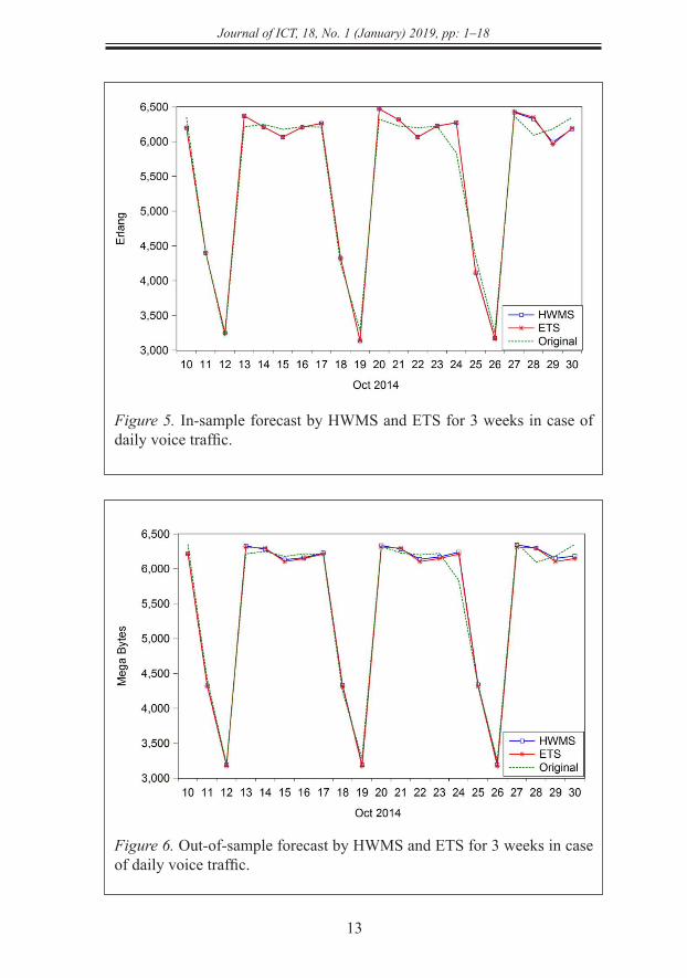
13
Journal of ICT, 18, No. 1 (January) 2019, pp: 1–18
Figure 5. In-sample forecast by HWMS and ETS for 3 weeks in case of daily voice traffic.
Figure 6. Out-of-sample forecast by HWMS and ETS for 3 weeks in case of daily voice traffic.
11
Figure 6. Out-of-sample forecast by HWMS and ETS for 3 weeks in case of daily voice traffic.
(3) Daily Data Traffic
The HWMS again is the best choice among other the simple exponential smoothing methods in the
case of daily data traffic due to the best RMSE of 48.03080, as presented in Table 6. Besides, AIC-
based ETS {A,N,M} was also the chosen model with the lower RMSE of 48.03521, as shown in
Table 7. The same results were achieved in the case of daily data traffic in which the HWMS and
ETS{A,N,M} have almost the same parameters, as in Table 8. The same is true for the same in-
sample forecasts in Figures 7 and 8 and the same out-of-sample forecast in Figure 9.
Table 6
Daily Data Traffic Estimation Outputs of Simple Exponential Smoothing Methods.
Exponential Smoothing Methods Single Double HWNS HWAS HWMS
Parameters Alpha 0.8080 0.1140 0.3200 0.6600 0.6700 Beta 0.0000 0.0000 0.0000 Gamma 0.0000 0.0000
Sum of Squared Residuals 2943240. 3114186. 2932171. 1040425. 1021982. Root Mean Squared Error 81.51002 83.84370 81.35660 48.46225 48.03080 End of Period Levels
Mean 1042.763 1117.194 1113.848 1093.138 1094.759 Trend 1.345373 1.359729 0.878545 0.878545
Table 7
Daily Data Traffic Estimation Output of AIC and AMSE Based ETS Chosen Models.
AIC Based AMSE Based Chosen Models E E{A} E{A}
10
Akaike Information Criterion Sum of Squared Residuals Root Mean Squared Error Average Mean Squared Error
66713129 531.6792
4269.541 66652447 531.4373 484775.5
Figure4. In-sample forecast by HWMS and ETS in case of daily voice traffic.
Figure 5. In-sample forecast by HWMS and ETS for 3 weeks in case of daily voice traffic.
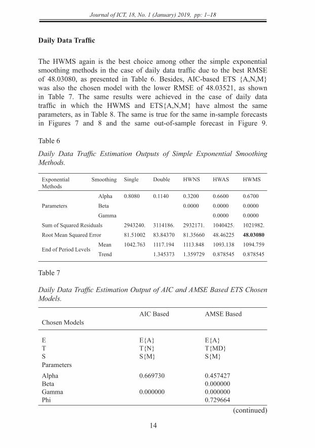
Journal of ICT, 18, No. 1 (January) 2019, pp: 1–18
14
Daily Data Traffic
The HWMS again is the best choice among other the simple exponential smoothing methods in the case of daily data traffic due to the best RMSE of 48.03080, as presented in Table 6. Besides, AIC-based ETS {A,N,M} was also the chosen model with the lower RMSE of 48.03521, as shown in Table 7. The same results were achieved in the case of daily data traffic in which the HWMS and ETS{A,N,M} have almost the same parameters, as in Table 8. The same is true for the same in-sample forecasts in Figures 7 and 8 and the same out-of-sample forecast in Figure 9. Table 6
Daily Data Traffic Estimation Outputs of Simple Exponential Smoothing Methods.
Exponential Smoothing Methods
Single Double HWNS HWAS HWMS
Parameters
Alpha 0.8080 0.1140 0.3200 0.6600 0.6700
Beta 0.0000 0.0000 0.0000
Gamma 0.0000 0.0000
Sum of Squared Residuals 2943240. 3114186. 2932171. 1040425. 1021982.
Root Mean Squared Error 81.51002 83.84370 81.35660 48.46225 48.03080
End of Period LevelsMean 1042.763 1117.194 1113.848 1093.138 1094.759
Trend 1.345373 1.359729 0.878545 0.878545
Table 7
Daily Data Traffic Estimation Output of AIC and AMSE Based ETS Chosen Models.
AIC Based AMSE BasedChosen Models
ETS
E{A}T{N}S{M}
E{A}T{MD}S{M}
ParametersAlphaBetaGammaPhi
0.669730
0.000000
0.4574270.0000000.0000000.729664
(continued)
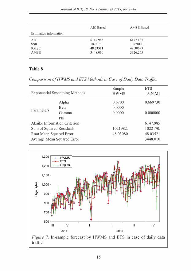
15
Journal of ICT, 18, No. 1 (January) 2019, pp: 1–18
AIC Based AMSE Based
Estimation information
AICSSRRMSEAMSE
6147.9851022170.48.035213448.010
6177.1371077010.49.306933326.265
Table 8
Comparison of HWMS and ETS Methods in Case of Daily Data Traffic.
Exponential Smoothing MethodsSimple ETSHWMS {A,N,M}
Parameters
AlphaBetaGammaPhi
0.67000.00000.0000
0.669730
0.000000
Akaike Information CriterionSum of Squared ResidualsRoot Mean Squared ErrorAverage Mean Squared Error
1021982.48.03080
6147.9851022170.48.035213448.010
Figure 7. In-sample forecast by HWMS and ETS in case of daily data traffic.
12
T S
T{N} S{M}
T{MD} S{M}
Parameters Alpha Beta Gamma Phi
0.669730 0.000000
0.457427 0.000000 0.000000 0.729664
Estimation information AIC SSR RMSE AMSE
6147.985 1022170. 48.03521 3448.010
6177.137 1077010. 49.30693 3326.265
Table 8
Comparison of HWMS and ETS Methods in Case of Daily Data Traffic.
Exponential Smoothing Methods Simple ETS HWMS {A,N,M}
Parameters
Alpha Beta Gamma Phi
0.6700 0.0000 0.0000
0.669730 0.000000
Akaike Information Criterion Sum of Squared Residuals Root Mean Squared Error Average Mean Squared Error
1021982. 48.03080
6147.985 1022170. 48.03521 3448.010
Figure 7. In-sample forecast by HWMS and ETS in case of daily data traffic.
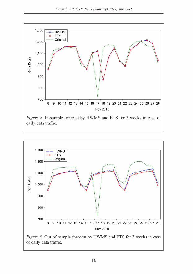
Journal of ICT, 18, No. 1 (January) 2019, pp: 1–18
16
Figure 8. In-sample forecast by HWMS and ETS for 3 weeks in case of daily data traffic.
Figure 9. Out-of-sample forecast by HWMS and ETS for 3 weeks in case of daily data traffic.
13
Figure 8. In-sample forecast by HWMS and ETS for 3 weeks in case of daily data traffic.
Figure 9. Out-of-sample forecast by HWMS and ETS for 3 weeks in case of daily data traffic.
CONCLUSIONS
In network planning and management, short-term prediction and real-time decisions are best served
by simple and low-cost prediction methods with a high accuracy. Therefore, exponential smoothing
methods, such as HWMS, were applied to forecast GSM/GPRS network Erlang traffic. However, a
more comprehensive study was required to evaluate the usage of various exponential smoothing
methods in more types of wireless traffic, such as data, which is becoming more important along with
the development of communication technology. This research applied different exponential smoothing

17
Journal of ICT, 18, No. 1 (January) 2019, pp: 1–18
CONCLUSION
In network planning and management, short-term prediction and real-time decisions are best served by simple and low-cost prediction methods with a high accuracy. Therefore, exponential smoothing methods, such as HWMS, were applied to forecast GSM/GPRS network Erlang traffic. However, a more comprehensive study was required to evaluate the usage of various exponential smoothing methods in more types of wireless traffic, such as data, which is becoming more important along with the development of communication technology. This research applied different exponential smoothing methods that were categorized as a simple exponential smoothing method and ETS framework, to forecast cellular network traffic that included voice and data. The experiments on hourly and daily traffic collected from commercial cellular networks showed that HWMS was the best fit for cellular network traffic among other simple exponential smoothing methods that included single, double, Holt-Winters No Seasonal, and Holt-Winters Additive Seasonal. It was unsuitable for the ETS framework to forecast hourly voice traffic. However, in the case of daily voice and data traffic, the ETS found that the {A,N,M} models provided nearly the same results as the HWMS. The HWMS forecast series was close to the original series in both hourly and daily voice traffic cases and showed a good ability to forecast daily data traffic as well. Due to the low complexity and low cost, HWMS can be applied effectively to cellular network traffic prediction. Moreover, the evaluation of HWMS can be further implemented based on the specific requirements of cellular networks.
ACKNOWLEDGMENT
This study was supported by National Natural Science Foundation of China (NSFC No.61271245).
REFERENCES
5G Vision. (2015). Retrieved from https://5g-ppp.eu/roadmapsFletcher, R. (1987). Practical methods of optimization (2nd ed.). New
York: John Wiley & Sons.Hyndman, R. J., Koehler, A. B., Snyder, R. D., & Grose, S. (2002). A state
space framework for automatic forecasting using Exponential smoothing methods. International Journal of Forecasting, 18(3), 439–454. doi: 10.1016/S0169-2070(01)00110-8
Margaret, V., & Jose, J. (2015). Exponential smoothing models for prediction of solar irradiance. International Journal of Advanced Research in
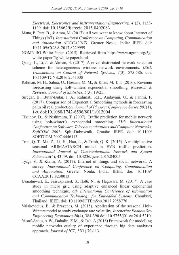
Journal of ICT, 18, No. 1 (January) 2019, pp: 1–18
18
Electrical, Electronics and Instrumentation Engineering, 4 (2), 1133-1139. doi: 10.15662/ijareeie.2015.0402083
Matta, P., Pant, B., & Arora, M. (2017). All you want to know about Internet of Things (IoT). International Conference on Computing, Communication and Automation (ICCCA2017). Greater Noida, India: IEEE. doi: 10.11.09/CCAA.2017.8229999
NGMN 5G White Paper. (2015). Retrieved from https://www.ngmn.org/5g-white-paper/5g-white-paper.html
Qiang, L., Li, J., & Altman, E. (2017). A novel distributed network selection scheme for heterogeneous wireless network environments. IEEE Transactions on Control of Network Systems, 4(3), 575-586. doi: 10.1109/TCNS.2016.2541338
Rahman, M. H., Salma, U., Hossain, M. M., & Khan, M. T. F. (2016). Revenue forecasting using holt–winters exponential smoothing. Research & Reviews: Journal of Statistics, 5(3), 19-25.
Siregar, B., Butar-Butar, I. A., Rahmat,. R.F., Andayani, U., & Fahmi, F. (2017). Comparison of Exponential Smoothing methods in forecasting palm oil real production. Journal of Physics: Conference Series,801(1), 1-9. doi:10.1088/1742-6596/801/1/012004
Tikunov, D., & Nishimura, T. (2007). Traffic prediction for mobile network using holt-winter’s exponential smoothing. 15th International Conference on Software, Telecommunications and Computer Networks, SoftCOM 2007. Split-Dubrovnik, Croatia: IEEE. doi: 10.1109/SOFTCOM.2007.4446113
Tran, Q. T., Ma, Z., Li, H., Hao, L., & Trinh, Q. K. (2015). A multiplicative seasonal ARIMA/GARCH model in EVN traffic prediction. International Journal of Communications, Network and System Sciences,8(4), 43-49. doi: 10.4236/ijcns.2015.84005
Tyagi, V., & Kumar, A. (2017). Internet of things and social networks: A survey. International Conference on Computing, Communication and Automation. Greater Noida, India: IEEE. doi: 10.1109/CCAA.2017.8230013
Usaratniwart, E., Sirisukprasert, S., Hatti, N., & Hagiwara, M. (2017). A case study in micro grid using adaptive enhanced linear exponential smoothing technique. 8th International Conference of Information and Communication Technology for Embedded Systems. Chonburi, Thailand: IEEE. doi: 10.1109/ICTEmSys.2017.7958776
Valakevicius, E., & Brazenas, M. (2015). Application of the seasonal Holt-Winters model to study exchange rate volatility. Inzenerine Ekonomika-Engineering Economics,26(4), 384-390.doi: 10.5755/j01.ee.26.4.5210
Yusuf-Asaju, A.W., Dahalin, Z.M., & Ta'a, A (2018) Framework for modelling mobile networks quality of experience through big data analytics approach. Journal of ICT, 17(1) 79-113.