CENTER FOR CI,)MPOSITE MATERIALS AND …")MPOSITE MATERIALS AND STRUCTURES ... _I_0/9311 GI_&I?tlI_I_/RBCII lntslil lte_o_t ... A time-dependent characterization study was performed

VIRGINIA TECH

CENTER FOR

"."/"_i_ Iv 7"--

IAJ _. >_ - _- I_

CCMS-88-02

VPI-E-88-5

CI,")MPOSITE MATERIALS

AND STRUCTURES

Radiation and Temperature Effectson the Time-Dependent Response

of T300/934 Graphite/Epoxy

Robert N. Yancey

Marek-Jerzy Pindera

9.... i.... 4

.... I

.... i

.... i

.... i

::::I_.... i.... i.... i.... | ...,.... i.... i ......... i ........ i ........ i ........ i ........ i ....

.... i ....

.... i ....

.... | ........ i ....

.... i ....

.... i ....

.... i ....

.... i ....

.... i ....

.... i ....

iiiiiiii::::1::::.... i ........ i ........ i ........ i ........ i ........ i ....

7,7,1','_',_,]::]]i[]]]_,,,,,,_1_i_,.... i ........ i ........ i ........ i ........ i ........ i ........ i ........ i ........ i ........ i ....

7,,

/,,/

?iiii::::!!i?

iii!i!ii_!iiii!iiiii!!ii!!

/

f

Virginia Polytechnic

Institute

and

State University

Blacksburg, Virginia

24061

(liiS/t-CI1-182503) a&DIATICII AIlI} TE/II_Rtli_:UBEtti]_C_S Cli 'Ztt_ TIet'-Dll_II_D]_fl _fS_OIIStl O¥_I_0/9311 GI_&I?tlI_I_/RBCII lntslil lte_o_t Iio.t$ {¥irginla Polytechnic l_st. and State

l.llziv. ) 171: p CSCL 110

1t88-18646

OnclasG3/2q 0129555

https://ntrs.nasa.gov/search.jsp?R=19880009262 2018-05-31T05:28:51+00:00Z

('ollege of EngineeringVirginia Polytechnic Institute and State UniversityBlacksburg, Virginia 24061

March 1988

CCMS-88-02VPI-E-88-5

Radiation and Temperature Effects

on the Time-Dependent Response

of T300/934 Graphite[Epoxy

Robert N. Yancey _Marek-Jerzy Pindera 2

Department of Engineering Science & Mechanics

Interim Report 69The NASA-Virginia Tech Composites ProgramNASA Grant NAG-1-343

Prepared for:

Applied Materials BranchNational Aeronautics and Space AdministrationLangley Research Centerttampton, Virginia 23665

t Graduate Student, Department of Engineering Science & Mechanics

Assistant Professor, Department of Engineering Science & Mechanics

Radiation and Temperature Effects on the Time-Dependent Response of T300/934 Graphite/Epoxy

(ABSTRACT)

A time-dependent characterization study was performed on T300/934 graphite/epoxy in a simulated

space environment. Creep tests on irradiated and non-irradiated graphite/epoxy and bulk resin

specimens were carried out at temperatures of 72 °F and 250 °F. Irradiated specimens were exposed

to dosages of penetrating electron radiation equal to 30 years exposure at GEO-synchronous orbit.

Radiation was shown to have little effect on the creep response of both the composite and bulk

resin specimens at 72 °F while radiation had a significant effect at 250 °F. A healing process was

shown to be present in the irradiated specimens where broken bonds in the epoxy due to radiation

recombined over time to form cross-links in the 934 resin structure. An analytical, micromechanical

model was also developed to predict the viscoelastic response of fiber reinforced composite materi-

als. The model was shown to correlate well with experimental results for linearly viscoelastic ma-

terials with relatively small creep strains.

Acknowledgements

This research was supported by the NASA-Virginia Tcch ('omposites l'rogram under Grant

NAG-I-343. The present investigation is a direct outgrowth of the work on radiation effects of

composites initiated by Professor Carl Herakovich and the late George Sykes of NASA I.angley

Research Center. Appreciation is expressed to Wayne Slemp and Joan Funk at NASA Langley

Research Center for their help in preparing the specimens. Appreciation is also expressed to Pro-

fessor Hal Brinson for the use of testing equipment located in the Laboratory for Experimental

Mechanics and Non-Metallic Materials Characterization at VPI & SU.

ooo

Acknowledgements nun

Table of Contents

1.0 Introduction ........................................................ I

1.1 Composites ......................................................... 1

1.2 Space Environment ................................................... 3

1.2.1 Vacuum ........................................................ 3

1.2.2 Temperature ..................................................... 4

1.2.3 Radiation ....................................................... 5

1.3 Background ........................................................ 6

1.3.1 Tensile Results ................................................... 6

1.3.2 Modified Epoxy and Cyclic Results ................................... 11

1.3.3 Compression and Bulk Resin Results .................................. 16

1.3.4 Conclusions .................................................... 16

1.4 Objectives ......................................................... 18

2.0 Experimental Investigation ............................................. 20

2.1 Test Matrix ....................................................... 20

2.2 Material .......................................................... 22

2.3 Specimen Preparation ................................................ 22

Table of Contents iv

2.4 Testing ........................................................... 27

2.4.1 Composite Creep ................................................ 27

2.4.2 Bulk Resin Creep ................................................ 27

2.5 Loading Sequence ................................................... 31

2.6 Data Acquisition .................................................... 36

3.0 Experimental Results ................................................. 37

3.1 Nomenclature ...................................................... 38

3.2 0° Results ......................................................... 38

3.3 Entire History Results ................................................. 40

3.3.1 10° Results ..................................................... 40

3.3.2 90° Results ..................................................... 43

3.4 Individual Results ................................................... 46

3.4.1 Bulk Resin Results ............................................... 49

3.4.2 10° Results ..................................................... 49

3.4.3 45° Results ..................................................... 52

3.4.4 90° Results ..................................................... 57

3.5 Lineatity .......................................................... 62

3.5.1 Linearity Verification .............................................. 62

3,5.2 Bulk Resin Linearity ................................. ............. 65

3.5.3 Composite Off-Axis Linearity ....................................... 65

3.5.4 Elastic Response ................................................. 74

3.6 Discussion ........................................................ 74

3.6.1 Healing Effects .................................................. 74

3.6.2 IE Linearity .................................................... 81

3.6.3 90° Recovery Discussion ........................................... 81

4.0 Analytical Model .................................................... 83

Table of Contents v

4.1 Linear Viscoelasticity ................................................. 84

4.2 Correspondence Principle ............................................. 87

4.2.1 Laplace Transform Conversion ...................................... 87

4.2.2 Boundary Value Problems .......................................... 88

4.3 Micromechanical Models .............................................. 90

4.3.1 Itashin Model ................................................... 91

4.3.2 Aboudi Model .................................................. 94

4.4 Application of Correspondence Principle .................................. 94

4.5 Matrix Modelhlg .................................................... 96

4.5.1 Parameter Evaluation ............................................ 100

4.6 Program Verification ................................................ 103

5.0 Experimental-Analytical Correlation ..................................... 114

5.1 Matrix Modeling ................................................... 114

5.2 Model Comparison ................................................. 115

5.2.1 Back Calculation ................................................ 115

5.2.2 Experimental-Analytical Correlation Results ............................ 124

5.2.3 IE Results .................................................... 124

6.0 Conclusions and Recommendations ...................................... 134

7.0 References ....................................................... 136

Appendix A. Bellman Method ............................................. 140

Appendix B. MICVIS User's Guide ......................................... 146

B. 1 Introduction ...................................................... 146

B.2 Input Description .................................................. 148

Table of Contents vi

B.3 Output Description ................................................ 151

Appendix C. Elastic Properties ............................................. 154

Table of Contents vii

List of Illustrations

Figure

Figure

Figure

Figure

Figure

Figure

Figure

Figt_e

Figure

Figure

Figure

Figure

Figure

Figure

Figure

Figure

Figure

Figure

Figure

Figure

Figure

1. Shifting of DMA Curves .......................................... 8

2. Results of DMA Test on T300/934 ................................... 9

3. TMA Results for T300/934 ....................................... 10

4. I0 ° Cyclic Room Temperature Axial Results ........................... 12

5. 10° Cyclic Elevated Temperature Axial Results ......................... 13

6. 10° Cyclic Room Temperature Shear Results .......................... 14

7. 10" Cyclic Elevated Temperature Shear Results ......................... 15

8. Tensile Results of 934 Resin ....................................... 17

9. Composite Tensile Specimen Dimensions ............................. 23

10. Photographs of Gripped Composite and Bulk Resin Specimens ............. 25

11. Photograph of Three-to-One Creep Frame ....................... . .... 28

12. Photograph of Ten-to-One Creep Frame ..................... ........ 29

13. Load Train for Composite Creep Frame .............................. 30

14. Bulk Resin Loading Assembly ..................................... 32

15. Photograph of Bulk Resin Loading Assembly ............. ............. 33

3416. Loading Sequence for All Tests ....................................

17. Local and Global Coordinate Systems ............................... 39

18. 10o Entire

19. 10° Entire

20. 10° Entire

21. 10° Entire

History Longitudinal Result Test at Room Temperature .......... 41

History Longitudinal Result at Elevated Temperature ............ 42

History Shear Results at Room Temperature ................... 44

History Shear Results at Elevated Temperature ................. 45

List of Illustrations viii

Figure

Figure

Figure

Figure

Figure

Figure

Figure

Figure

Figure

Figure

Figure

Figure

Figure

Figure

Figure

Figure

Figure

Figure

Figure

Figure

Figure

Figure

Figure

Figure

Figure

Figure

Figure

! :igure

22. 90° Entire History Longitudinal Results at Room Temperature ............. 47

23. 90° Entire I listory Longitudinal Results at Elevated Temperature ............ 48

24. Bulk Resin Results at 1.60 KSI .................................... 50

25. Bulk Resin Results for Entire Loading History ......................... 51

26. 10° Off-Axis Longitudinal Results at 7.26 KSI .......................... 53

27. 10° Off-Axis Longitudinal Results at 14.85 KSI ......................... 54

28. 10° Off-Axis Shear Results at 7.26 KSI ............................... 55

29. 10° Off-Axis Shear Results at 14.85 KSI .............................. 56

30. 45 ° Off-Axis Longitudinal Results at Initial Loading ..................... 58

31. 45 ° Off-Axis Longitudinal Results at Final Loading ...................... 59

32. 45° Off-Axis Shear Results at Initial Loading ........................... 60

33. 45° Off-Axis Shear Results at Final Loading ........................... 61

34. 90° Longitudinal Results at 1.21 KSI ................................ 63

35. 90° Longitudinal Results at 2.42 KSI ................................ 64

36. Example Creep Response for I,inearity Verification Procedure .............. 66

37. Example Isochronous Lines for Linearity Verification Procedure ............ 67

38. NR Bulk Resin Linearity Verification ................................ 68

39. IR Bulk Resin Linearity Verification ................................. 69

40. NE Bulk Resin Linearity Verification ................................ 70

41. NR 10° Off-Axis Linearity Verification ............................... 71

42. IR 10° Off-Axis Linearity Verification ................................ 72

43. NE 10° Off-Axis Linearity Verification ............................... 73

44. Effect of Pre-Soak Time at 250 °F on Creep Response ................... 80

45. Single Composite Cylinder ........................................ 92

46. Hashin Composite Cylinder Assemblage Model ......................... 93

47. Aboudi Micromechanical Model .................................... 95

48. Power Law Graphical Representation ............................... 98

49. Mechanical Representation of Four-Parameter Model ................... 99

List ofIllustrations ix

Figure

Figure

Figure

Figure

Figure

Figure

Figure

Figure

Figure

Figure

Figure

Figure

Figure

Figure

Figure

Figure

Figure

Figure

Figure

Figure

Figure

i :igurc

Figure

Figure

50. Parameter Determination for Power-Law Model ....................... 102

51. Parameter Determination for Four-Parameter Model .................... 104

52. MICVIS Aboudi Model Prediction and Exact Value .................... 106

53. MICVIS Hashin Model Prediction and Exact Value .................... 107

54. SI1 Compliance vs. Time ........................................ 108

55. S12 Compliance vs. Time ........................................ 109

56. $66 Compliance vs. Time ........................................ 110

57. $22 Compliance Bounds vs. Time ................................. 111

58. $44 Compliance Bounds vs. Time ................................. 112

59. Linear Viscoelastic Model Approximations to NR Bulk Resin Data ......... 116

60. Linear Viscoelastic Model Approximations to IR Bulk Resin Data .......... 117

61. Linear Viscoelastic Model Approximations to NE Bulk Resin Data ......... 118

62. Linear Viscoelastic Model Approximations to IE Bulk Resin Data .......... 119

63. 10° Longitudinal Experimental-Analytical Correlation ................... 125

64. 10° Shear Experimental-Analytical Correlation ........................ 126

65. 45 ° Longitudinal Experimental-Analytical Correlation ................... 127

66. 45 ° Shear Experimental-Analytical Correlation ........................ 128

67. 90° Longitudinal Experimental-Analytical Correlation ................... 129

68. 10° IE Longitudinal Experimental-Analytical Correlation ................. 131

69. 45° IF, Shear FxpcrimentM-Analytical Correlation ...................... 132

70. 90° IE Longitudinal Experimental-Analytical Correlation ................. 133

71. Sample Input File for MICVIS .................................... I50

72. Sample Output for ttashin Model .................................. 152

73. Sample Output for Aboudi Model ................................. 153

List of Illustrations x

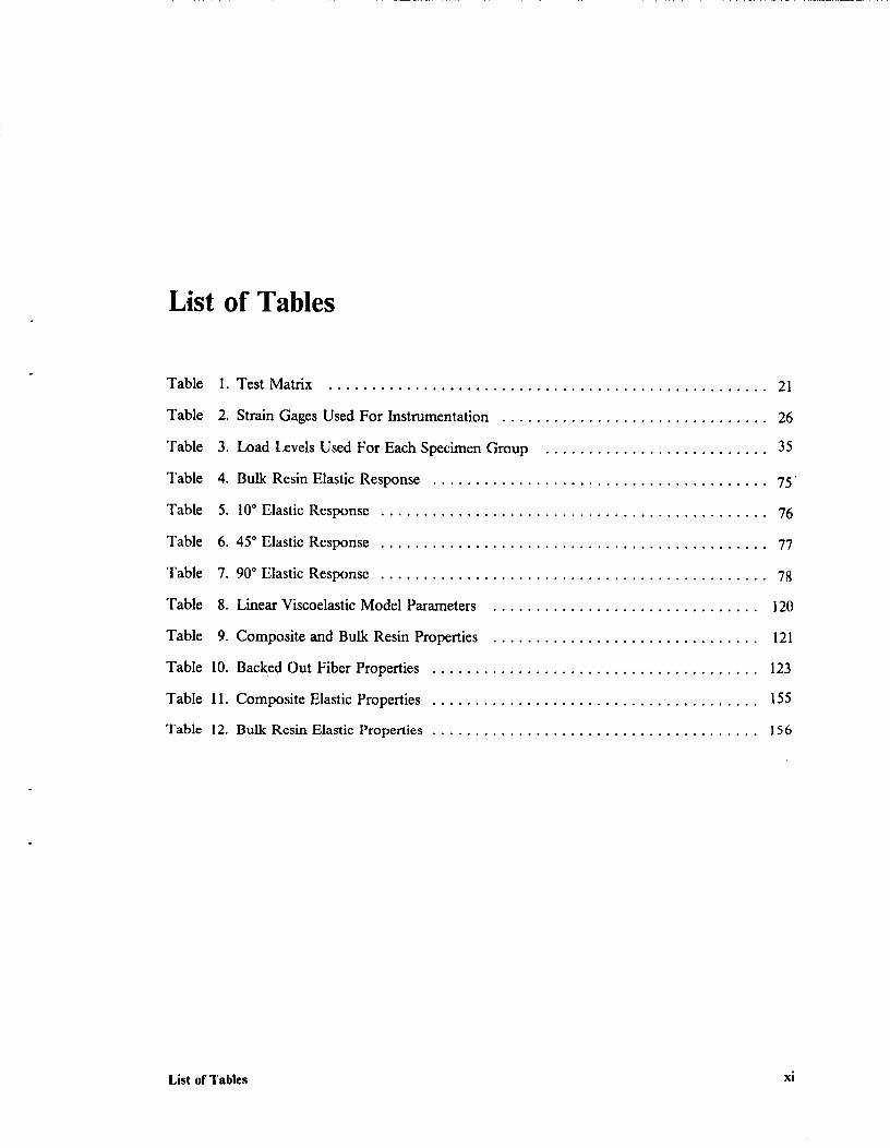
List of Tables

Table 1. Test Matrix ................................................... 21

Table 2. Slrain Gages Used For Instrumentation ............................... 26

Table 3. Load Levels Used For Each Specimen Group .......................... 35

Table 4. Bulk Resin Elastic Response ....................................... 75

Table 5. 10 ° Elastic Response ............................................. 76

Table 6. 45 ° Elastic Response ............................................. 77

Table 7. 90* Elastic Response ............................................. 78

Table 8. Linear Viscoelastic Model Parameters ............................... 120

Table 9. Composite and Bulk Resin Properties ............................... 121

Table 10. Backed Out Fiber Properties ...................................... 123

Table 11. Composite Elastic Properties ...................................... 155

Table 12. Bulk Resin Elastic Properties ...................................... 156

List of Tables xi

1.0 Introduction

1.1 Composites

The use of resin-matrix composites has become quite commonplace in the aerospace field today.

Much of the truss structure of the proposed space station will be made of graphite/epoxy [1]. l ligh

Technology Communication Satellites and future Space Platlbrms such as tile Space Telescope

would be virtually impossible without composites [2-7]. These projects are a result of an increased

awareness of the advantages composite materials offer. The most commonly mentioned advantages

are superior strength-to-weight and stiffness-to-weight ratios but other advantages are beginning to

surface. Some of these additional advantages are low thermal conductivity, low thermal expansion

with the ability to eliminate it completely, and the ability to tailor composites to specifically meet

certain needs. Engineers now look to composite materials not only to save weight but to design

structures that meet requirements that were previously thought unrealistic with more common

materials such as metals mad plastics. Good dimensional stability and high specific damping char-

acteristics make composites an excellent choice for projects such as the Space Telescope and com-

munication satellites [1]. With the advent of sophisticated computer codes that can deal with the

complexities involved in the analysis of composite materials, design engineers see the unlhnitcd

Introduction I

potential they have to design extremely sophisticated and efficient structures [8]. Composite mate-

rials are changing the entire approach to structural design.

Although we have come a long way in understanding composite materials, problems and challenges

still exist with many of these materials. Resin matrix composites such as graphite/epoxy are pres-

ently the most widely used advanced composites. This type of composite is lirnited in most cases

by the resin itself which has a limited operating temperature range and properties that can change

noticeably within this range. The resin can also age with time and become embrittled [9-11]. An-

other characteristic of polymer resins is creep. Epoxy resins are made up of long molecular chains

that are cross-linked together to form a complicated molecular structure. The cross-linking is highly

irregular throughout the internal structure and this allows chains to bend, slide, twist, and curl

around each other. Chemical bonds are constantly broken and reformed and as a result, the

structure never remains the same. When a tensile load is applied to a polymer, kinks in the mo-

lecular chains are quickly straightened which produces an instantaneous deformation. This is usu-

ally referred to as the elastic response. If the load remains, however, these chains slowly begin to

slide, twist and uncurl causing more dcformation. Tiffs time-dependent deformation is known as

creep [12,13]. Creep presents unique problems to design engineers since they must not only design

a structure to withstand present loads and displacements but must also consider the given loads and

displacements over the design lifetime of the structure. The structure is no longer "rigid" but is

constantly displacing and dissipating energy. This introduces complexities into the design of di-

mensionally stable structures. Much work has been done to help designers better quantify the creep

characteristics of resins and more importantly resin matrix composites [14]. Some of this work,

paying special attention to the effects of the space environment on creep behavior, will be discussed

below.

I ntroduction 2

1.2 Space Environment

Structural designers need to pay special attention to the extremes of the space environment when

designing space structures. These environmental factors can seriously affect structural integrity of

resin matrix composites. The space environment has many conditions not commonly regarded in

tile design of earth-bound structures. The major environmental factors that need to be considered

in space are vacuum, temperature cycling, and radiation. These factors are most pronounced in

high earth orbits such as GEO-synchronous orbit. Previous work dealing with the effect of these

environmental extremes on resin matrix composites is outlined below.

1.2.1 Vacuum

All space environments are characterized by near vacuum. Although this is often seen as advanta-

geous since it helps eliminate corrosive environments and can decrease structural degradation, it is

a major concern with resin matrix composites. Moisture, along with small trapped organic mole-

cules such as carbon monoxide (CO) and carbon dioxide (C02) that have been separated from the

polymer chains of the epoxy, can "outgas" from the polymer network drying out and embrittling

the epoxy [9]. This outgassing can also cause voids to form, thus disrupting the molecular structure

of the resin. These voids can be of two types. First, they can be small intemal voids left behind

by the space occupied by the outgassed molecule. This increases the free volume of the epoxy

which can facilitate movement of the molecular chains and thereby increase the amount that the

material will creep over time [14,15]. Secondly, if outgassing occurs within the composite, larger

voids can develop in the composite network. Gas pockets can form within the structure causing

delaminations and matrix cracking both of which can significantly affect the composite strength and

stiffness [16,171.

Introduction 3

1.2.2 Temperature

The space environment is also characterized by large temperature fluctuations. Since the environ-

ment is a near vacuum, there are few particles that can hold heat. For tiffs reason, the temperature

in space is almost entirely dependent on whether the region is in the sun's path or blocked from its

rays. Orbiting structures can experience temperatures as high as + 250 °F when in the light and

heat of the sun and as low as -250 °F when blocked from the sun's rays.

The temperature extremes and temperature cycling experienced by orbiting spacecraft can seriously

affect resin matrix composites due to the dissimilar thermal properties of the composite constitu-

ents. The coefficient of thermal expansion of a resin is quite different than that of a stiff fiber such

as graphite. With a temperature change, the resin in bulk form will expand or contract differently

than a graptfite fiber under the same conditions. Since the composite is a rigid structure composed

of fibers and resin, an expansion or contraction compromise is reached by the two components.

As a result, each component compensates for the expansion or contraction deficiency with a me-

chanical load. For example, a graphite/epoxy composite when cooled will experience, in the di-

rection of the fibers, a mechanical tensile load in the matrix and a mechanical compressive load in

the fibers. In a free and unconstrained state, the matrix upon cooling contracts significantly and the

graphite fiber expands slightly i 18]. Being constrained by each other in the composite, the fiber and

matrix are restricted in their respective expansion or contraction. The result is tension in the matrix

and compression in the fiber. With tiffs behavior, thermal cycling actually results in mechanical

load cycling of the resin and fibers. This load cycling can fatigue the structure at the fiber-rcsin level

which often results in microcracking of the resin matrix I19].

Temperature can also have an effect on the epoxy network itself. Temperature increases the motion

of molecular chains in the epoxy allowing for a less rigid molecular structure which facilitates creep

[201. The increased motion coupled with the increased free volume created by outgassing can sig-

nificantly increase the ability of the molecules to slide, twist, and uncurl.

Introduction 4

1.2.3 Radiation

Another significant factor in the space environment is radiation. There are many types of radiation

in space and the types change depending on the location in orbit. Several types of radiation expe-

rienced in high-earth orbits are not significant at low-earth orbits. At high-earth orbits, low energy

radiation such as visible and ultraviolet light is present along with charged particles such as electrons

and protons, and high energy radiation such as cosmic, gamma and x-rays [21,22]. Low energy

forms of radiation are believed to have little if any effect on resin matrix composites. High energy

forms of radiation can affect surface properties of materials but are unable to penetrate significantly

into the material. Charged particles, if accelerated to high speeds, can penetrate the structure and

cause damage. These charged particles seem to damage the polymer resin structure more adversely

than they do stiff fibers such as graphite. Graphite fibers have been shown to be essentially inert

to all forms of radiation [231.

Most scientists conclude that the main effect of radiation is chain scission and separation of low

molecular weight products such as radicals and ionic centers from the epoxy network. Chain

scission increases the mobility of molecular chains and also enhances disentanglement of the low

molecular weight chains formed 1261. The increased chain mobility mad disentanglement can cause

chain slippage which manifests itself as creep behavior [26,27]. Along with molecular chain move-

ment, unstable radicals present in the irradiated epoxy will eventually recombine. Recombination

of radicals is highly dependent on chain mobility. At low temperatures, the radicals produced by

radiation are quite immobile and remain trapped in the structure. As temperature increases, the

radicals move more freely which allows them to recombine. Based on thermal cycling and Dynamic

Mechanical Analysis (DMA) data, Tenney, Sykes, and Bowles [21] proposed that all the radicals

will recombine eventually and that temperature accelerates this activity. Recombination of radicals

results in increased cross-linking creating a more rigid structure but one more brittle as wcU

[21,22,261.

Introduction 5

1.3 Background

Much work has been done at Virginia Tech to quantify the effects of the space environment on

T300/934 graphite/epoxy. The work was initiated by Herakovich and Sykes and they conducted

separate studies with Milkovich, Reed, and Fox. A brief summary of their work is given below,

emphasizing the results leading to the present study.

1.3.1 Tensile Results

Milkovich, llcrakovich, and Sykes 116] studied the effects of radiation and temperature on the

tensile response of T300/934 graphite/epoxy. Quasi-static monotonic tensile tests were performed

on unidirectional coupons with fiber orientations of 0°, 10°, 45°, and 90°. Three temperatures were

used, namely cryogenic (-250 °F), room (+ 72 °F), and elevated (+ 250 °F). Half of the specimens

were subjected to electron radiation representative of 30 years in GEO-synchronous orbit. For the

0° coupons, radiation had little effect on stiffness. Radiation combined with elevated temperature,

however, significantly reduced the strength. For the 90° coupons, radiation lowered the strength

for all three test temperatures and lowered the stiffness at elevated temperature. For the 10° and

45 ° off-axis coupons, radiation had a significant effect on strength at the elevated temperature but

little effect on stiffness. For the 10°, 45 °, and 90° coupons, radiation at elevated temperature greatly

increased the onset of nonlinear behavior in tile stress-strain response.

Milkovich, et al. 1161 also performed a Dynamic Mechanical Analysis (DMA) and Thermo Me-

chanical Analysis (TMA) on irradiated and non-irradiated specimens. The DMA test is a way to

dctcrmine the glass transition temperature (7_) by monitoring damping of the polymcr as a function

of temperature. Determination of how the glass transition temperature changes indicates the state

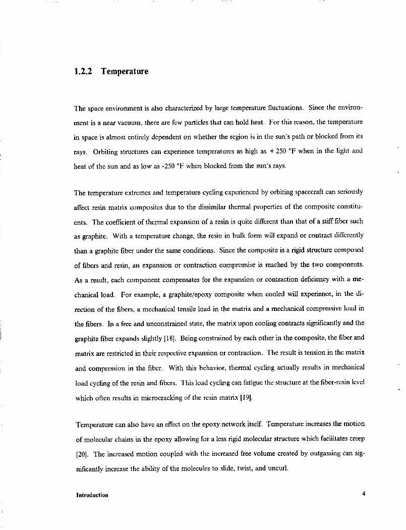
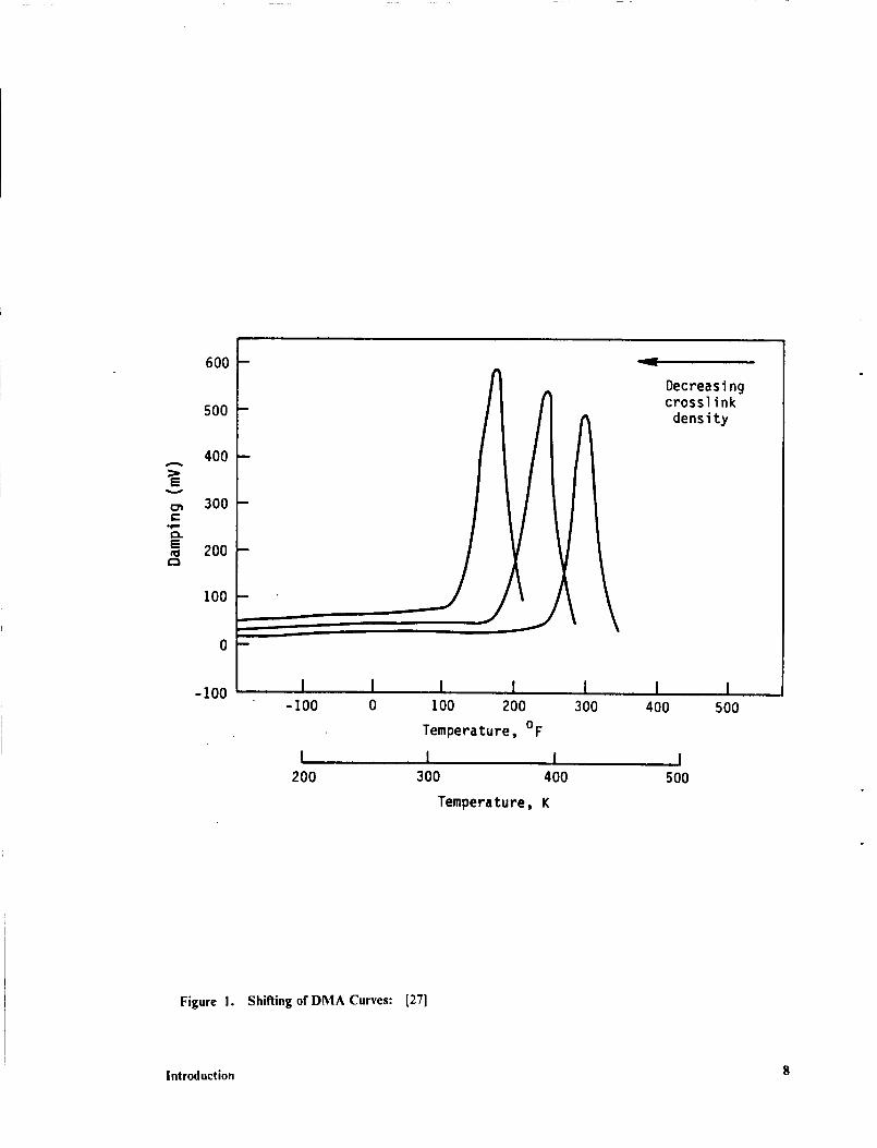
of the epoxy molecular chain network. As shown in Figure 1, reduction in the glass transition

Introduction 6

temperatureindicates reduction in the cross-link density. An increase in the magnitude of the

damping peek indicates reduction in the average molecular weight of the molecular chains wlffch

represents the average size of the molecules in the network. Widening of the peek curve indicates

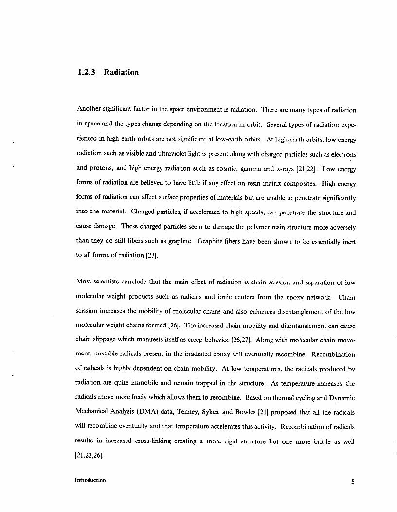
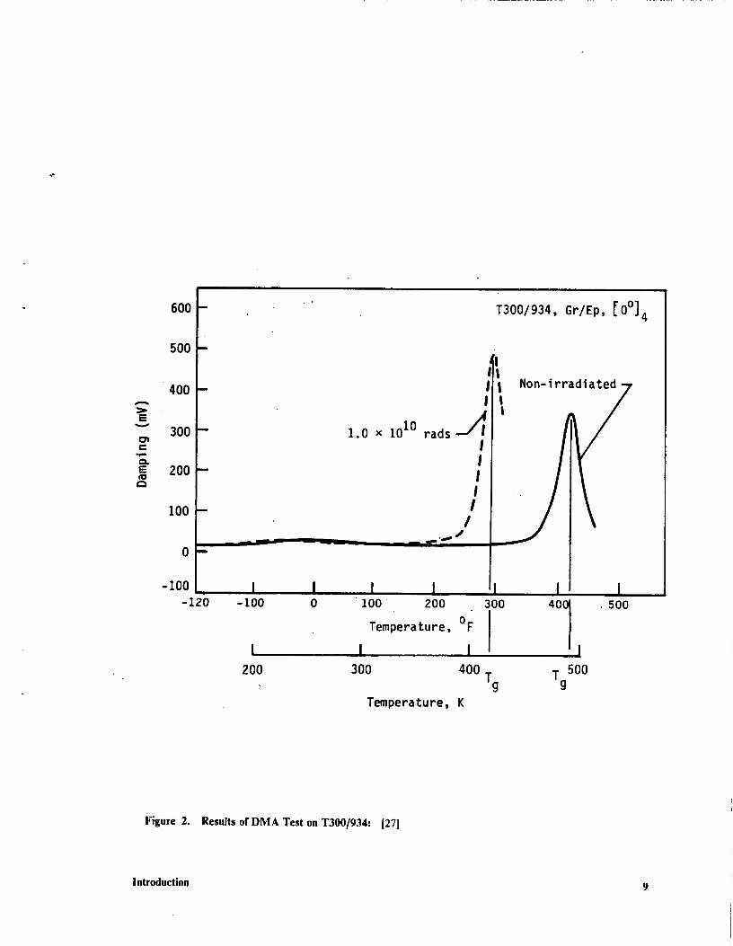
greater distribution of molecular weights. Tests of the baseline and irradiated specimens indicated

that radiation resulted in the reduction of cross-link density and average molecular weight. Radi-

ation also increased the distribution of molecular weights. Figure 2 illustrates these results.

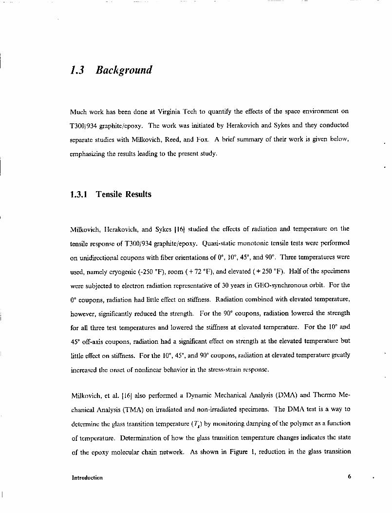
The TMA test evaluates the relative softness of a material with respect to temperature. A probe

is lightly spring-loaded onto the specimen and its penetration is monitored as a function of tem-

perature. The results of the TMA tests performed by Milkovich, et al. 116] show that irradiation

softened the material at lower temperatures indicating both a lowering of the Ts and in increase in

the creep behavior. This is shown in Figure 3. The anomaly at the end of the TMA curve is due

to the probe being pushed away from the irradiated specimen at elevated temperature due to de-

laminations caused by low molecular weight products boiling off.

Milkovich, et al. [16] concluded that irradiation affected only the epoxy resin and had little effect

on the graphite fibers, tle also concluded that radiation resulted in chain scission of the epoxy

network which serves to weaken the epoxy resin. The mechanism described by Milkovich, et al.

1161is one in which small molecular groups are broken off from the main chains due to radiation.

These small molecules tend to "freeze" the structure at low temperatures creating a stiffer structure.

At high temperatures, these molecules boil off and "plasticize" the material. Milkovich, et al. [16]

concluded that tiffs mechanism explains the nonlinear behavior seen at elevated temperatures in the

irradiated condition.

Introduction 7

A

E

e-

E

6OO

50O

400

3OO

2OO

100

-100-IO0

/ /i

I200

I II00 200

Temperature, OF

I I300 400

Temperature, K

Decreasingcrosslink

density

3OO 400 500

I500

Figure I. Shifting of DMA Curves: [27]

Introduction 8

A

e-,r.=

E

r_

400

30O

200

100 --

0"

-100

-120

Gr/Ep, [0 °]4T300/934,

I-100

1.0 x 1010 rads

L_____J L_____0 100 " 200

OTemperature, F

I I I200 300 400

Temperature, K

I

i Non-irradiated 7

3O0

Tg

40( .500

I

Tg 500

Figure 2. Results of DMA Test on T300/934: [27]

Introduction 9

,e,-E

O

e-

XW

CO

ww_

$.

GI

2.0

1.5

1.0

.5

-0.5

-I .0

I

I T300/934, GrlEp

4-ply, unidirectionalI

I

I

Ii

1.0 x 1010 rads-_

III

I

I

I

I

.II

I

Non-i_radiated -_ II

I I I I100 200 300 400

Temperature, OF

I I

3OO 400

Temperature, K

500

Figure 3. TMA Results for T300/934: [27]

Introduction i0

1.3.2 Modified Epoxy and Cyclic Results

Reed, Herakovich, and Sykes [23] continued the investigation of Milkovich, et al. [16] and at-

tempted to verify one conclusion of that investigation. Milkovich, et al. [ 16] concluded that small

molecules broken off during irradiation were a result of additives used in the processing of the epoxy

resin and not an inherent property of the epoxy resin itself. Milkovich, et al. [16] proposed to

eliminate the additive and thus solve the problem. In order to verify Milkovich's hypothesis, Reed,

et al. [23] performed the same tests with a modified T300/934 graphite/epoxy where the processing

additives had been left out during the manufacturing process. Little difference was seen with the

results of Reed, et al. 123] in comparison with Milkovich, et al. [16]. It was concluded that the ra-

diation was affecting the epoxy network itself.

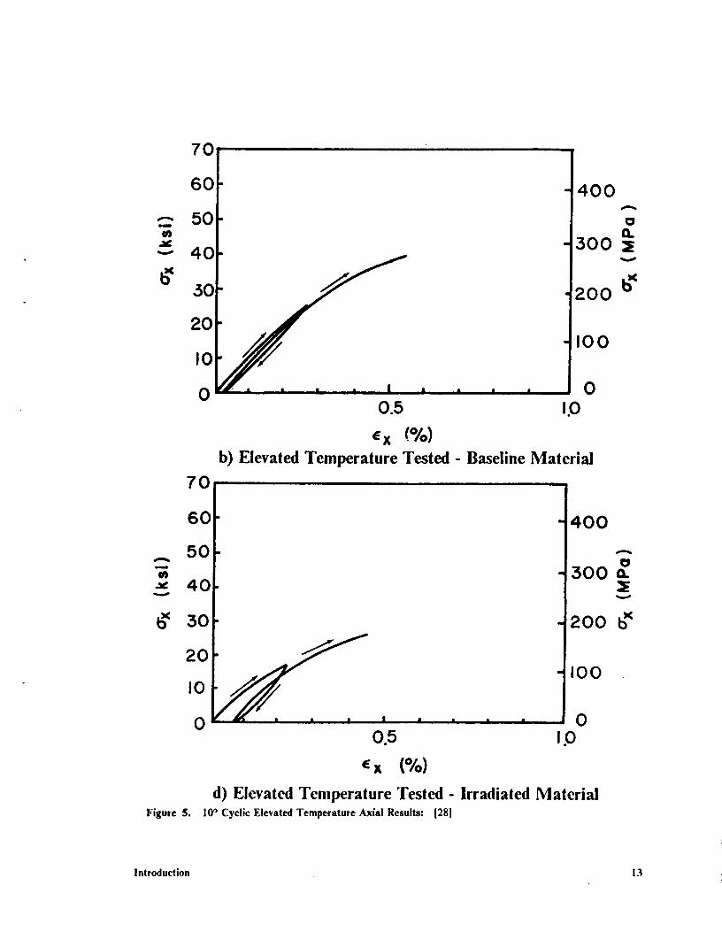
Reed, et al. [23] also performed cyclic tension tests on the original (unmodified) epoxy composite

investigated by Milkovich, et al. [16]. Each specimen was subjected to quasi-static loading beyond

the linear range, subsequent unloading to zero, and finally immediate re-loading to failure. These

tests were conducted to evaluate better the nature of the nonlinear behavior observed by Milkovich,

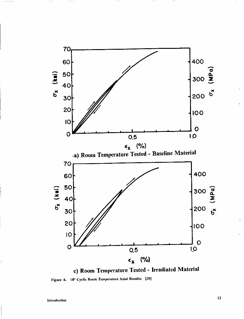
et al. [16]. Figure 4 and Figure 5 show sample results of the longitudinal cyclic response of the

10° off-axis specimen under various conditions of temperature and radiation. As seen, hysteresis

is present in the response for all conditions and the second and fmal loading does not proceed

through the reversal point of the loading/unloading cycle. If the nonlinear behavior observed by

Milkovich, et al. [16] were purely plastic, the re-loading response should pass through the reversal

point of the preceding cycle. The fact that in this case the reloading proceeds as it does suggests

that viscoelastic behavior is present. The irradiated coupons at elevated temperature have a much

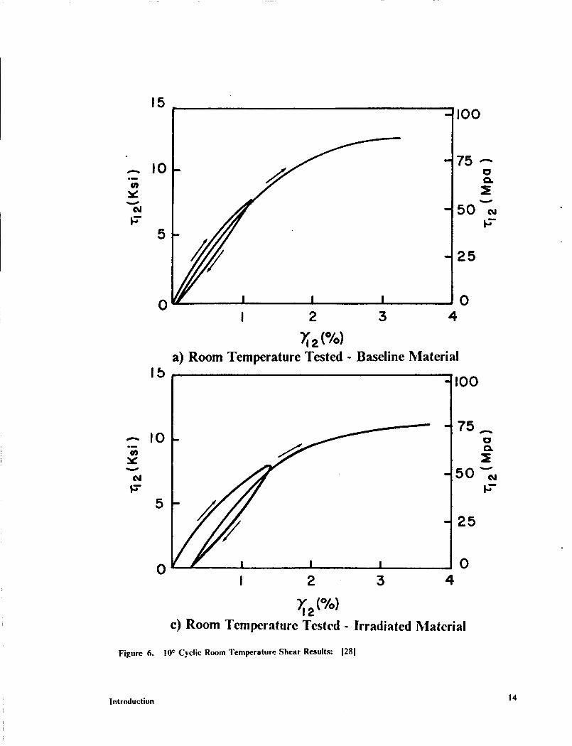
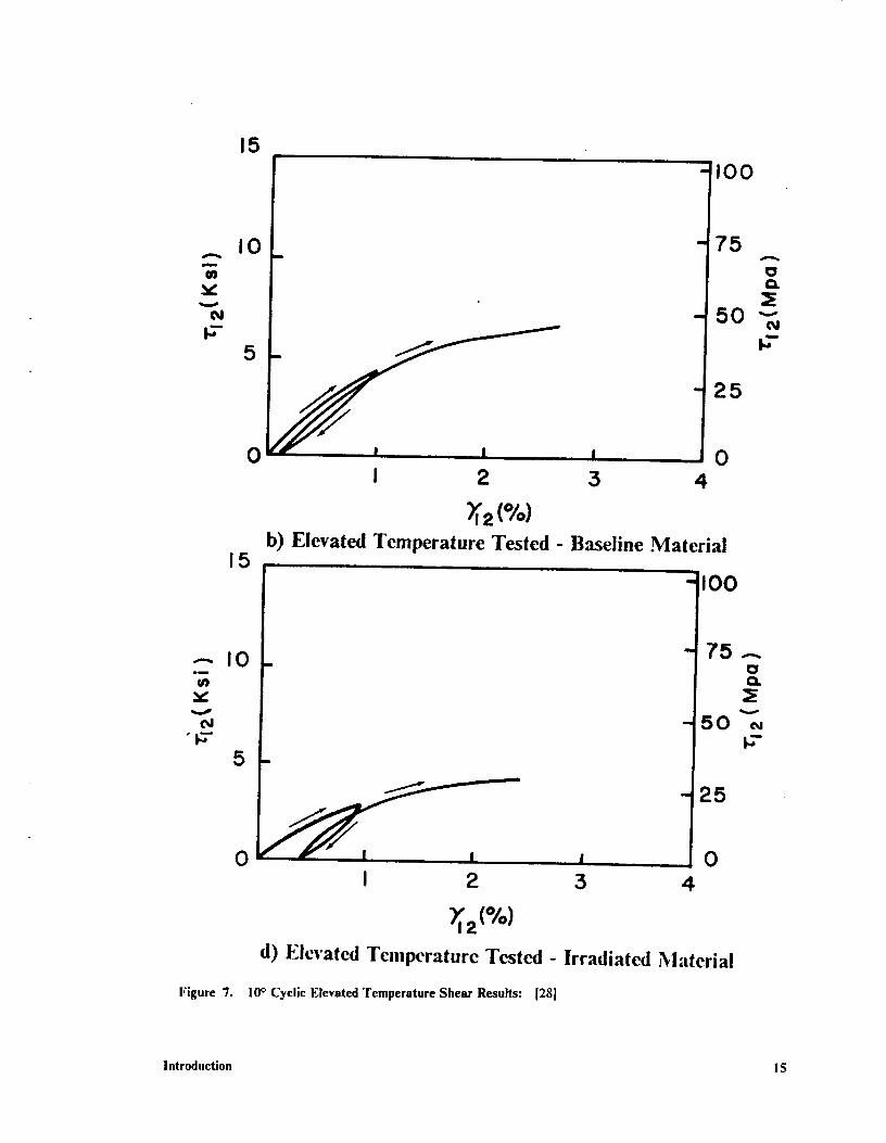
larger hysteresis indicating a greater contribution of viscoelastic behavior. Figure 6 and Figure 7

show the shear response in the material principal coordinate system of the 10° off-axis specimen.

For shear, the hysteresis is larger in all cases indicating that the viscoelastic response is dominant

in shear.

Introduction I I

7(

60 400

4o 300

_' 30 200 b"

20 I00

I0 0

0 0.5 1.0

_x (%),a) Root== Temperature Tested - Baseline Material

_o[---_-W-- _601- f "t 400

•= 300

./J l'OO.-A_,OOo

0 0.5 1.0

_x (%)

c) Room Temperature Tested - Irradiated Material

Figure 4. 10 ° Cyclic Room Temperature Axial Results: 128]

Introduction 12

7O

60 400A

oem,

e_

40 300

20_ J J,O0

0 0.5 1.0

x (%)b) Elevated Temperature Tested - Baseline Material

:;t 4 oo3oI- -12oo b"

0.5 ip

x (%)

d) Elevated Temperature Tested - Irradiated MaterialFigure 5. 10 ° Cyclic Elevated Temperature Axial Results: [28]

Introduction 13

15

_. I0

5

0

15

I 2 .3 4

_2(%)a) Room Temperature Tested - Baseline Material

I0

0I 2 3 4

7_2(%)c) Room Temperature Tested - Irradiated Material

Figure 6. 10 ° Cyclic Room Temperature Shear Results: 128l

I00

50 ,_

25

0

I00

5o ,_

25

0

!ntroduction 14

15

m

ol

5

0

15

AIOo_

01v

(M,_--.

5

0

Figure 7.

I

I 2 3

-100

- 75

a.:E

- 50 v(q

- 25

_04

b) Elevated Temperature Tested - Baseline Materiali

"I00

- 75A" I_

Q.

-50

- 25J 0

I 2 3 4

21%)d) Elevated Temperature Tested - Irradiated Material

10° Cyclic Elevated Temperature Shear Results: [28]

Introduction i 5

Reed, et at. [23] performed additional tests on the graphite fibers alone. Radiation was shown to

have little if any effect on the strength or stiffness of the fibers.

1.3.3 Compression and Bulk Resin Results

Fox, Herakovich, and Sykes [26] continued the investigation into radiation and temperature effects

on the T300/934 composite system by examining the compressive properties under the same con-

ditions as those employed by Milkovich, ct at. 116] and Reed, et al. [23]. The results show shnilar

reductions in stiffness and strength observed by Milkovich, et al. [161. Bulk resin tests were also

conducted. The trends of these results agree favorably with the composite tensile results. These

results are shown in Figure 8. At elevated temperature in the irradiated condition, reduction in

strength coupled with nonlinear behavior is observed. This further supports the conclusion that the

radiation significantly affects the epoxy resin which contributes to the response of the composite.

Fox,et al. [26], Reed, et at. [23], and Milkovich [16], et at. all concluded that chain scission due to

radiation is the principal degradation mechanism in the epoxy resin. These conclusions are drawn

mainly from the DMA and TMA data and appear to explain many of their results.

1.3.4 Conclusions

The effects of radiation on the 934 resin system seem to correlate well with previous work done on

radiation effects of polymers. Chain scission and the formation of radicals is consistent with the

DMA and TMA results obtained by Milkovich, et al. [16]. This effect would indeed decrease the

cross-link density and average molecular weight of the epoxy network, thus initially increasing the

viscoelastic behavior observed by Reed, et al. 1231. Chain scission and low molecular weight pro-

ducts win increase chain mobility and thus facilitate creep behavior. At temperatures near the Ts,

the chains are very mobile and substantial viscoelastic behavior is present. In the irradiated condi-

Introduction 16

12

BASELINE

--- U_I_J) IA'I'EU

+ 250

'8O

"80

"ZO

0

4

Figure 8. Tensile Results of 934 Resin: [29]

Introduction 17

tion, + 250 °F is very close to the Ts. The increase in viscoelastic behavior would increase the ap-

parent onset of nonlinear behavior seen by Milkovich, et al. [16] and Fox, et al. [26].

The tests carried out by Milkovich, et al. 116], Reed, et al. 123], and Fox, et al. 1261were all quasi-

static in nature. Their results do correlate with the literature on radiation effects of polymers. The

literature also suggests, however, that these radicals will recombine over time to form cross-links.

Due to their short-term duration, quasi-static tests of the type performed by Milkovich, et al. [16],

Reed, et al. [23], and Fox, et al. [261 give very little information on this phenomena. Time-

dependent tests of a longer duration will clarify this occurrence by monitoring the deformation as

a function of time, temperature, and radiation. They will also help to quantify the viscoelastic be-

havior of T300/934 graphite/epoxy.

1.4 Objectives

The objectives of this study are two-fold. The first objective is to quantify the effects of radiation

and temperature on the time-dependent behavior of T300/934 graphite/epoxy. In order to meet this

objective, creep tests on irradiated and non-irradiated graphite/epoxy specimens were carried out

at two test temperatures, namely + 250 °F and + 72 °F. Penetrating electron radiation was chosen

since it seems to have the most significant effect on resin matrix composites [16,23,26]. Creep tests

were conducted on different fiber orientations of the graphite/epoxy under these varying conditions.

Creep tests were also carried out on the bulk 934 resin. The goal was to better understand how

radiation and temperature affected the matrix dominated creep response of this composite system.

The second objective of this study is to develop a time-dependent predictive tool for fiber reinforccd

composite materials with the aid of the micromechanics approach. In this approach, the composite

is viewed at the level of a single fiber. Micromechanical models, as now formulated, are able to

Introduction 18

predict composite elastic properties from the constituent elastic properties. To accomplish the

objective of this study, existing micromechanical models were modified by use of the Correspond-

ence Principle to predict composite viscoelastic properties from constituent viscoelastic properties.

This allows designers to combine computationaUy many different materials to fred the one that has

the viscoelastic properties he or she desires.

!ntroduction 19

2.0 Experimental Investigation

This chapter discusses the techniques and procedures employed in the experimental portion of this

investigation. The discussion will begin with a presentation of the test matrix and a description of

the specimen preparation techniques. The specimen preparation techniques used in this study are

identical to those used by Milkovich, et al. [271, Reed, et al. [28], and Fox, et al. [29] and more de-

tailed descriptions of these procedures can be found in the above references. A detailed discussion

of the various testing machines and testing equipment will then be presented. This chapter will

conclude with a discussion of the data acquisition systems used to gather the necessary information.

2.1 Test Matrix

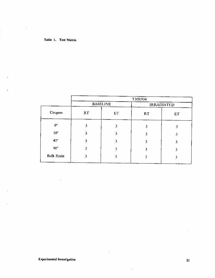
Table 1 shows the test matrix used for this study. Tensile creep tests were conducted on

unidirectional coupons with fiber orientations of 0°, 10°, 45°, and 90°. These are the same fiber

orientations used by Milkovich, et al. [271, and Reed, et al. [28]. Bulk resin creep tests were also

performed.

Experimental Investigation 20

TableI. TestMatrix

T300/934

BASELINE IRRADIATED

Coupon RT E'F RT ET

o

10°

45 °

90°

Bulk Resin

3

3

3

3

3

3

3

3

3

3


Creep tests are a common method to characterize the time-dependent response of a material. A

creep test consists of an instantaneous loading of a specimen to a given load level, maintaining that

load level for a given time, and monitoring the deformation as a function of time. A perfectly elastic

material in a creep test will exhibit an instantaneous strain which then remains constant with time.

A time-dependent material in a creep test will also exhibit an instantaneous strain but then the

strain will increase with time. The manner in which the strain increases characterizes the time-

depcndcnt response of the material.

2.2 Material

The material used in this study was T300/934 graphite/epoxy. T300 is a graphite fiber made by

Thornel (Union Carbide) and 934 is a thermoset epoxy resin. An eight-ply panel and a four-ply

panel were manufactured according to standard procedures [27-29].

2.3 Specimen Preparation

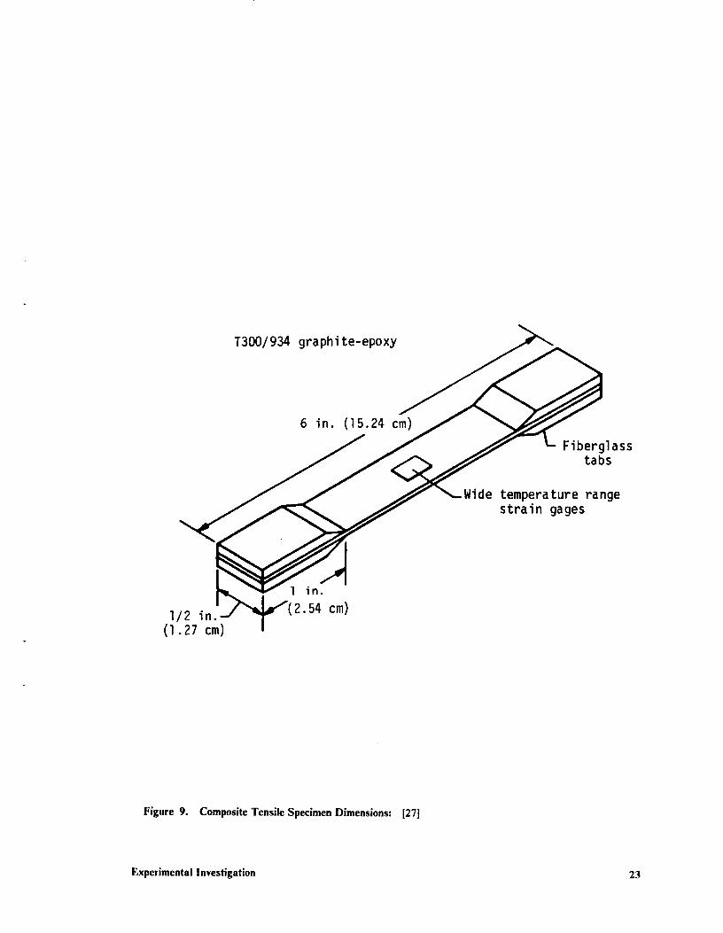
Both panels were C-scanned to check for large voids or flaws and none were detected. The speci-

mens were cut from the panels to the dimensions of 6" x 0.5" (152.4 mm x 12.7 mm). This di-

mension was chosen to optimize the number of specimens that could be placed in the irradiation

facility without overly compromising the specimen aspect ratio. The specimen dimensions are

shown in Figure 9. The 0° and 45° specimens were cut from a single eight-ply panel at VPI & SU.

The 10° and 90 ° specimens were cut from a single four-ply panel at NASA Langley Research

Center. The edges were all visually inspected for smoothness and parallel alignment.


T300/934 graphite-epoxy

6 in. (15.24 cm)

Fiberglasstabs

Wide temperature range

strain gages

I/2 in.

(1.27 cm)

1 in.

2.54 cm)

Figure 9. Composite Tensile Specimen Dimensions: [27]


After machining, half of the specimens were subjected to electron radiation in the radiation facility

at NASA langley Research Center. The specimens were irradiated with 1 MeV electrons at a dose

rate of 50 Mrads/hr for 200 hours. This yielded a total dose rate of 10,000 Mrads which is equiv-

alent to 30 years exposure in GEO-synchronous orbit. The 10° and 90° degree coupons were

irradiated together in the same batch and the 0° and 45° coupons were irradiated in a separate batch.

The specimens were tabbed with 1.25" x 0.5" (31.8mm x 12.7mm) fiberglass at each end. The tabs

were beveled at 30 degrees and applied at NASA Langley Research Center using standard tabbing

procedures [28].

The bulk resin specimens were manufactured according to procedures outlined by Fox [291. The

specimen shape was tile smaU "dog-bone" specimen (type V) from ASTM Standard D638-82a 1301.

A photograph of the gripped composite and bulk resin specimens is shown in Figure 10.

All the specimens were instrumented with strain gages. The strain gages were applied with AE-15

adhesive which was cured at 120 *F for 6 hours under 15 psi pressure. Due to the fact that tem-

perature accelerates the recombination of radicals in the epoxy network, 120 °F was chosen as the

adhesive cure temperature so as to not expose the specimens to relatively high temperatures for long

periods of time while still allowing the adhesive to cure properly. A temperature of 120 °F is the

lowest adhesive cure temperature recommended by the adhesive manufacturer [31]. qqais also fol-

lows the strain gaging procedure used by Milkovich, et al. [27], Reed, et al. [28], and Fox, et al. [29].

Table 2 shows the gages used for each specimen group. After curing the adhesive, all gages were

measured for misalignment using a microscope available at VPI & SU.

All specimens were held under vacuum for at least five days prior to testing. Specimens were re-

moved from the vacuum chamber immediately before testing. It should be noted that the specimen

preparation techniques used by Milkovich, et al. [271, Reed, et at. [28], and Fox, et al. [29] were all

followed for this study. More detailed descriptions of specimen preparation can be found in those

references.


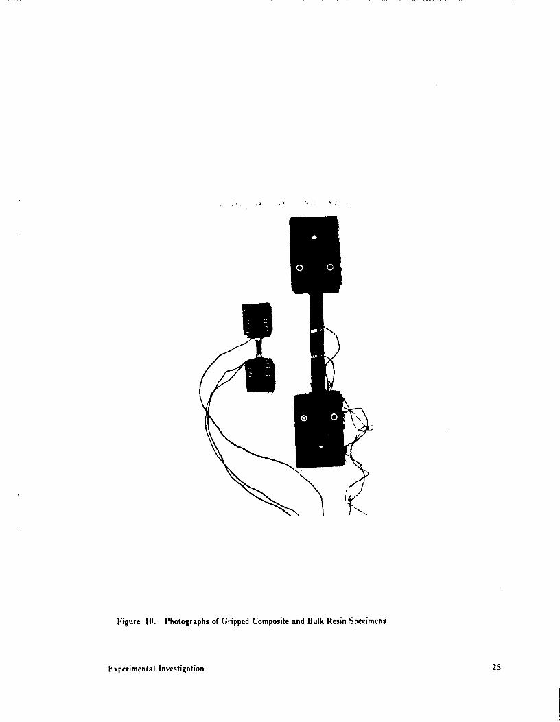
Figure !0. Photographs of Gripped Composite and Bulk Resin Specimens


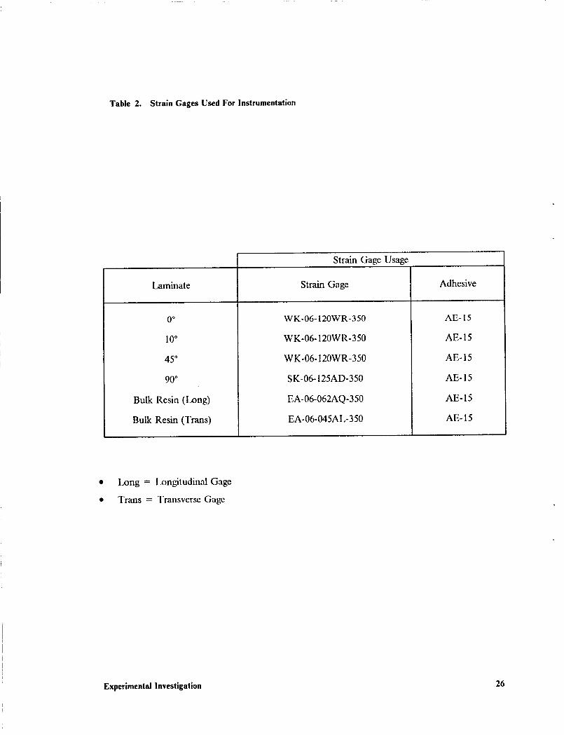
Table 2. Strain Gages Used For Instrumentation

Laminate

0 °

10°

45°

90°

Bulk Resin (Long)

Bulk Resin (Trans)

Strain Gage Usage

Strain Gage

WK-06-120WR-350

WK-06-120WR-350

WK-06-120WR-350

SK-06-125AD-350

EA-06-062AQ-350

EA-06-045AL-350

Adhesive

AE-15

AE-15

AE-15

AE-15

AE-15

AE-15

• Long = l._ngitudinal Gage

• Trans = Transverse Gage


2.4 Testing

2.4.1 Composite Creep

The 10°, 45*, and 90 ° tensile creep tests were performed on either a three-to-one or ten-to-one lever

arm creep frame, both of which are located at VPI & SU. The three-to-one creep frame had a

motor which gently released the weight to apply the load. The ten-to-one creep frame had a

manual crankshaft which lowered the weight to apply the load. Photographs of these two creep

frames are shown in Figure 11 and Figure 12. The specimens were gripped with steel grips that

were tightened with socket-head cap screws. The alignment in the grips was checked with a square

rule and marks on the grips were used for centering. Load was applied with steel pins going through

the grips and the load frame. A schematic of this is shown in Figure 13. The 0° tensile creep tests

were conducted on a United Testing Systems (UTS) screw-driven, load controlled testing machine

located at VPI & SU.

2.4.2 Bulk Resin Creep

The bulk resin creep tests were performed using a dead weight fixture designed by Signor [321 and

modified by the author. The grips designed by Fox, et al. [29] were also used in the present inves-

tigation. The load train consisted of the grips with pins, the specimen, 20 lb. test nylon line, a two

foot steel rod, and a load pan.

The nylon line was used to shorten the distance between the eye bolt and the base in case the

specimen broke while loading. The steel loading rods were aligned at the base of the frame with

cardboard inserts. The cardboard satisfactorily aligned the rods without significantly increasing the


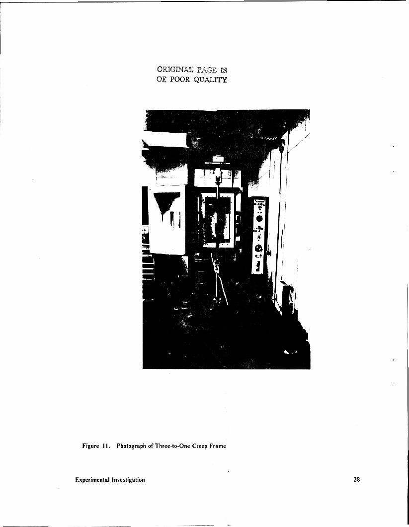
Figure 11. Photograph of Three-to-One Creep Frame


•OR.IGI_'qAL PAGE I_J

_-00R QUALITy

Figure 12. Photograph ofTen-to-One Creep Frame

Experimental investigation 29

Lever Arm

ps

Specimen

J

_Weigh'f. ______x_,_k_,_=." --

Pon

Figure 13. Load Train for Composite Creep Frame


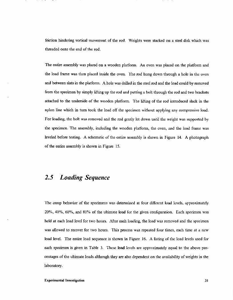
friction hindering vertical movement of the rod. Weights were stacked on a steel disk wtfich was

threaded onto the end of the rod.

The entire assembly was placed on a wooden platform. An oven was placed on the platform and

the load frame was then placed inside the oven. The rod hung down through a hole in the oven

and between slats in the platform. A hole was drilled in the steel rod and the load could by removed

from the specimen by simply lifting up the rod and putting a bolt through the rod and two brackets

attached to the underside of the wooden platform. The lifting of the rod introduced slack in the

nylon line which in turn took the load off the specimen without applying any compressive load.

For loading, the bolt was removed and the rod gcntly let down until the weight was supported by

tile specimen. The assembly, including the wooden platform, the oven, and the load franle was

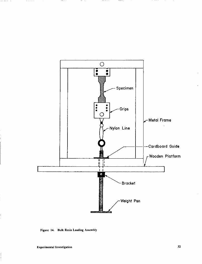
leveled before testing. A schematic of the entire assembly is shown in Figure 14. A photograph

of the entire assembly is shown in Figure 15.

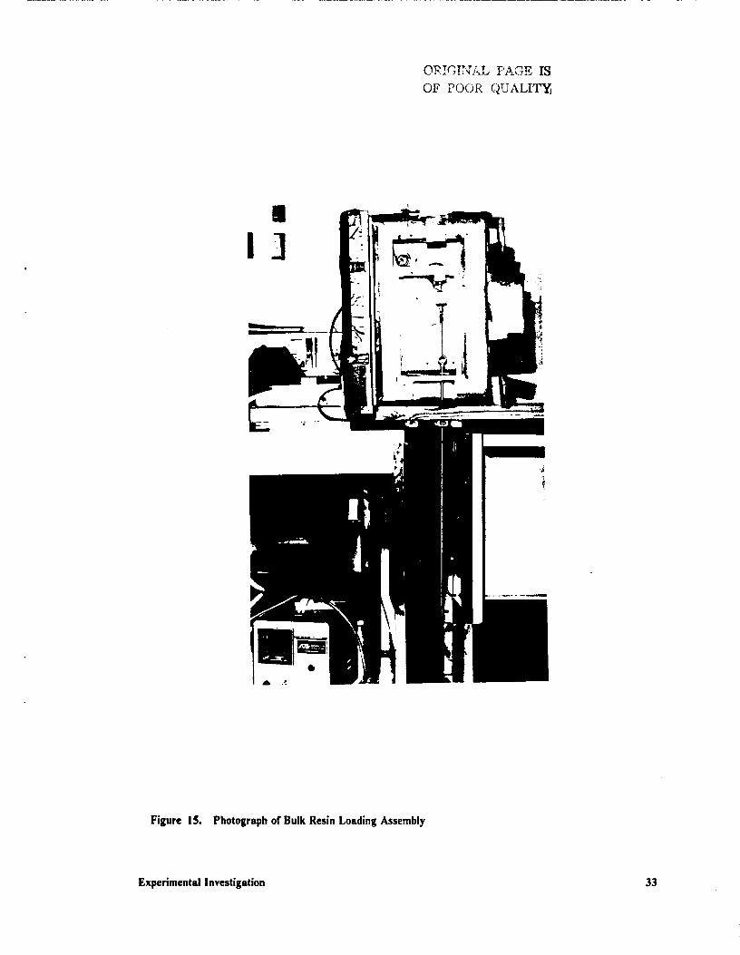
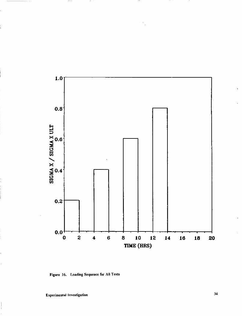
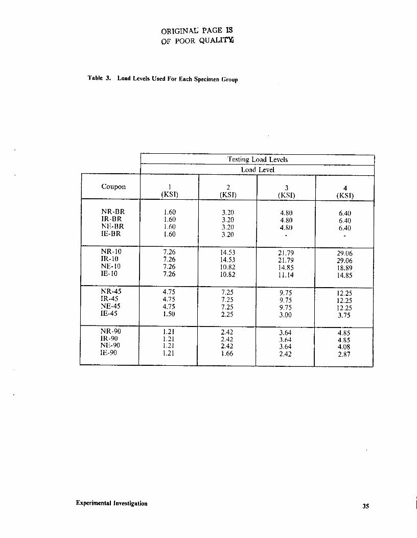
2.5 Loading Sequence

The creep behavior of the specimens was determined at four different load levels, approximately

20%, 40%, 60%, and 80% of the ultimate load for the given configuration. Each specimen was

held at each load level for two hours. After each loading, the load was removed and tile specimen

was allowed to recover for two hours. This process was repeated four times, each time at a new

load level. The entire load sequence is shown in Figure 16. A listing of the load levels used tbr

each specimen is given in Table 3. These load levels are approximately equal to the above per-

centages of the ultimate loads although they are also dependent on the availability of weights in the

laboratory.


0• •• •

Specimen

©Grips

Nylon Line

Frame

--Cardboard Guide

Platform

Bracket

ht Pan

Figure 14. Bulk Resin Loading Assembly


OR!GIICAL EAGE IS

OF POOR QUALIT_j

|

I]

Figure 15. Photograph of Bulk Resin Loading Assembly


1.0

0.00 2 4 6 8 10 12

TIME (HRS)

14 16 18 2O

Figure 16. Loading Sequence for All Tests


ORIGINAI5 PAGE IS

OF POOR QUALIT_

Table 3. Load Levels Used For Each Specimen Group

Testing Load Levels

Load Level

Coupon I 2 3 4

(KSI) (KSI) (KSI) (KSI)

NR-BRIR-BRNE-13RIE-BR

NR-10IR-10NE-101E-10

NR-45IR-45NE-45IE-45

NR-90IR-90NE-901E-90

1.601.601.601.60

7.267.267.267.26

4.754.754.751.50

1.211.21i.211.21

3.203.203.203.20

14,5314.5310.8210.82

7.257.257.252.25

2.422.422.421.66

4.804.804.80

21.7921.7914.8511.14

9.759.759.753.00

3.643.643.642.42

6.406.406.40

29.0629.0618.8914.85

12.2512.2512.253.75

4.854,854.082.87


2.6 Data Acquisition

Data for the 10°, 45 °, 90 °, and bulk resin tests was acquired with an Orion Data Acquisition System

interfaced with an IBM-AT personal computer. The data acquisition system was driven by a

software package entitled MATPACO. l"tfis is very similar to the software package MATPAC2

developed by Llidde [33]. MATPACO has the capability to vary the intervals at which data is taken

while the test is running. This capability was used to increase the data a.;quisition intervals as the

test progressed so that sufficient data was obtained without creating data ['des so large as to be un-

manageable. After loading and recovery, the data acquisition was halted and the system, including

the strain gages, was reinitialized. Tiffs was done to permit each loading and recovery to be saved

in a separate fde. After the data was recorded it was corrected for transverse sensitivity and gage

misaligruraent. Data for the 0° tensile creep tests was taken in a similar :fashion with an IBM-XT

personal computer interfaced with a Data Translation I)T2805/5716 A/D, D/A board and a Vishay

2100 system signal conditioner/amplifier.

Temperature for the elevated temperature tests was monitored with a theImocouple attached to the

grips holding the test specimen. Generally, the temperature was kept between 245 °F and 255 °F

yet the temperature rarely fluctuated more then 1-2 °F for each test. Temperature was not moni-

tored for the room temperature tests but all tests were run in temperature controlled rooms that

were kept at between 72 °F and 75 °F. Although humidity varied from day to day, all tests were

conducted on specimens fleshly removed from the vacuum chamber.


3.0 Experimental Results

The presentation of the experimental results will begin with a discussion of the nomenclature used

for the descriptions of the data presented in this chapter. A brief discussion on the outcome of the

0 ° tests will be followed by a presentation of entire history plots for the 10° and 90° results at room

temperature and elevated temperature. These results show general trends of the composite under

the loading sequence described in Section 2.5. Following a discussion of the general behavior of

these results, individual plots will be presented for all four conditions at a given load level. This

further illustrates the effect of temperature and radiation on the creep response of the composite

and bulk resin specimens. Since the results were consistent, a representative test is presented for

each condition. No smoothing or averaging of the test data was performed and all plots represent

actual test data. A discussion on linearity of the results will also be presented. Lineafity will be

an important assumption in Chapter 4.0 and will be discussed in more detail in Section 3.5. This

chapter will end with a discussion of the healing process of the epoxy resin and its effect on the

results. This phenomena is able to give acceptable explanations to the results that will now follow.

Experimental Results 37

3.1 Nomenclature

The nomenclature used to identify the tests will be discussed below. The testing conditions will

be hereafter identified by a two letter code. The first letter refers to the specimen condition. N

stands for non-irradiated and I for irradiated. The next letter refers to the test temperature. R

stands for room temperature and E stands for elevated temperature, l'he four conditions will

therefore be referred to as NR (non-irradiated room temperature), IR (irradiated room temper-

ature), NE (non-irradiated elevated temperature), and IE (irradiated elevated temperature).

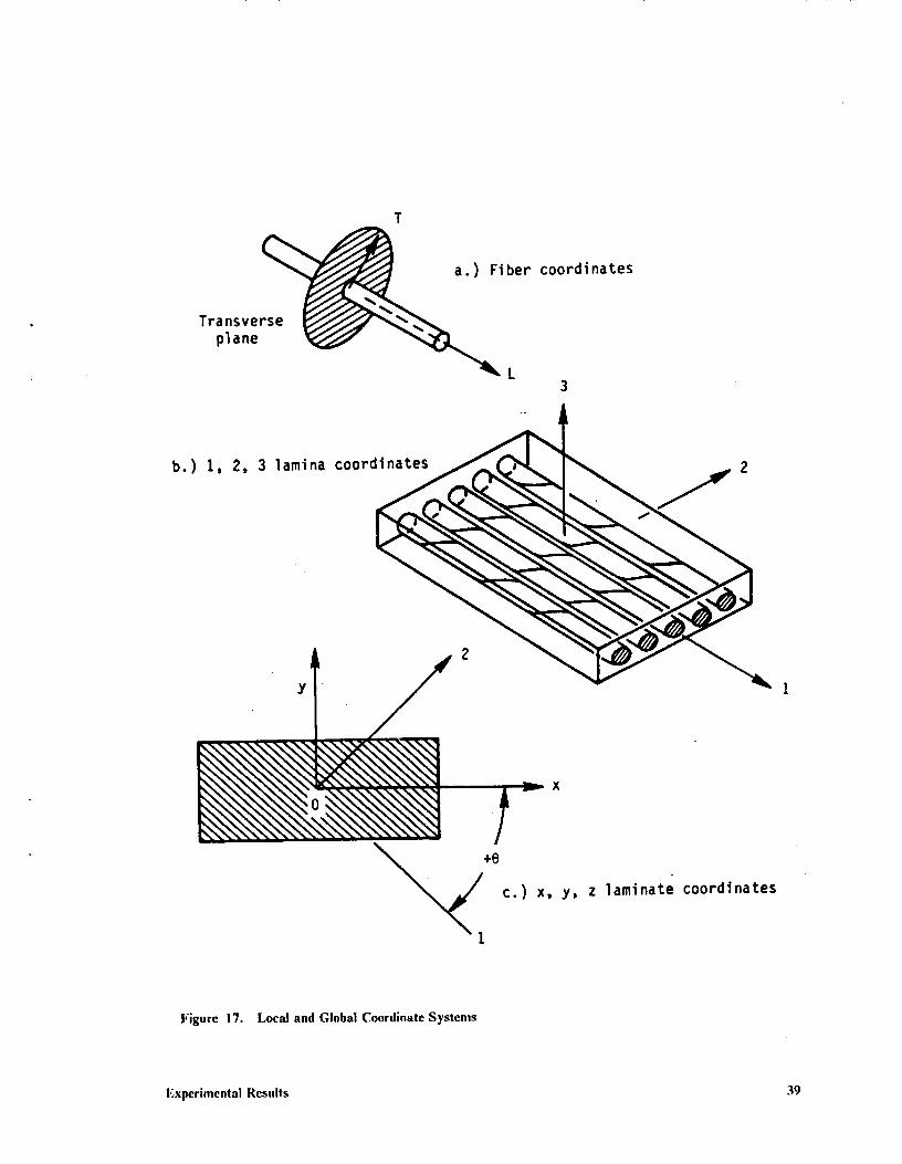
When refcrring to stresses and strains, standard notation will be used to differentiate between global

coordinates and material principal coordinates. Global coordinates will be referred to as the x-y-z

coordinates while material principal coordinates will be referred to as the 1-2-3 coordinates. Global

coordinates refer to the coordinate system of the test coupon where the e,aordinate axes are parallel

to the coupon edges. The material principal coordinates refer to the coordinate system of the

unidirectional composite where the coordinate axes are parallel and transverse to the fibers. This

is illustrated in Figure 17.

3.2 0 ° Results

In order to obtain a complete time-dependent material characterizatior, of the T300/934 system,

tensile creep tests were carried out on 0° coupons. These specimens exhibited no observable creep

in the time frame tested. Accurate elastic properties of the 0° coupons w,:re obtained, however, and

these properties will be used in Section 5.2.1.


T

ber coordinates

Transverse

plane

_L 3

, , coor I

b.) I 2 3 lamina

• y ' .

X

c.) x, y, z laminate coordinates

Figure 17. Local and Global Coordinate Systems


3.3 Entire History Results

3.3.1 10 ° Results

Figure 18 shows the longitudinal response for the entire loading history of the 10° off-axis tensile

coupon at room temperature. The load levels for both specimens are identical. The creep response

for the irradiated and non-irradiated specimens is nearly the same except for a slight difference in

the elastic response. Differences in the elastic response may be due to actual changes in the material

but may also be due to slight variations in the cross-sectional area of individual specimens. It is

seen that a slight permanent strain remains after the loading/recovery cycle at each load level for

both conditions.

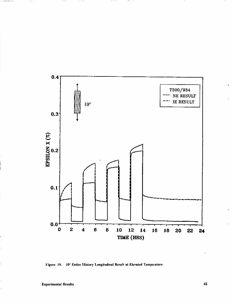
Figure 19 shows the longitudinal creep response for the entire loading history of the 10° off-axis

tensile coupon at elevated temperature. The load levels in this case are not the same for both

conditions due to the much lower ultimate stress of the IE specimens. It can be seen, however, that

the creep response for the irradiated condition is unlike the response for the non-irradiated condi-

tion. The creep response for the non-irradiated condition looks similar to the room temperature

results. The creep response for the irradiated condition is quite different. The initial creep response

is significant and its corresponding recovery exhibits a large permanent strain. As the test

progresses, the magnitude of the creep behavior for the IE condition appears to diminish with

subsequent loading. The recovery after each loading seems to exhibit less permanent strain than

the recoveries of previous loadings. The final recovery strain of the IE condition, however, shows

a large permanent strain. As shown, the final recovery strain value upon completion of the test is

much different than the initial strain value of zero strain.

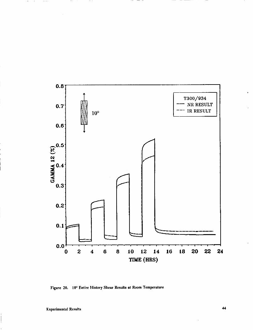
Figure 20 and Figure 21 show the i-2 shear response for the entire loading history of the 10° off-

axis tensile coupon. Figure 20 shows the room temperature results and Figure 21 shows the ele-


0.4'

0.3'

A

x

Z

o0.2'

0.1'

10°

00. • ' • ' " .....0 2 4 6 8

f

T300/934

NR RESULT

IR RESULT

__mm_mmmmw_m_

J,

| | = | - ! • | - s '-

10 12 14 16 18 20 22 24

TIME (HRS)

Figure 18. 10 ° Entire History Longitudinal Result Test at Room Temperature


0.4'

0.3

A

0.1

10 °

T300/934

_m NE RESULT

--- IE RESULT

i

_ m

U e | - | . s . e - i - m .w o

• | | • u - a -

0 2 4 6 8 10 12 14 16 18 20 22 2,4

TIME (HRS)

I:igure 19. 10 ° Entire llistory I,ongitudinal Result at Elevated Temperature


vated temperature results. The same trends can be seen here, but in a much more pronounced

fashion. The room temperature results show similar behavior for both the irradiated and non-

irradiated conditions except for the elastic response. The recovery in both cases exhibits a smaU

permanent strain. The elevated temperature results show a dramatic difference in the two re-

sponses. The non-irradiated condition shows similar behavior to the room temperature results

while the irradiated condition shows a very large creep deformation. Upon recovery, the IE con-

dition shows a significant permanent strain. As in Figure 19, the permanent strain diminishes with

subsequent loadings yet the final permanent strain upon completion of the test is almost as great

as the strain attained by the NE coupon at the highest load level. It should be noted that tile fmal

load level for the IE test is less than the f'mal load level for the NE test. These results suggest that

the creep behavior of the epoxy resin is most critical in shear. This is supported by the 90 ° creep

test data discussed in the subsequent section.

3.3.2 90 ° Results

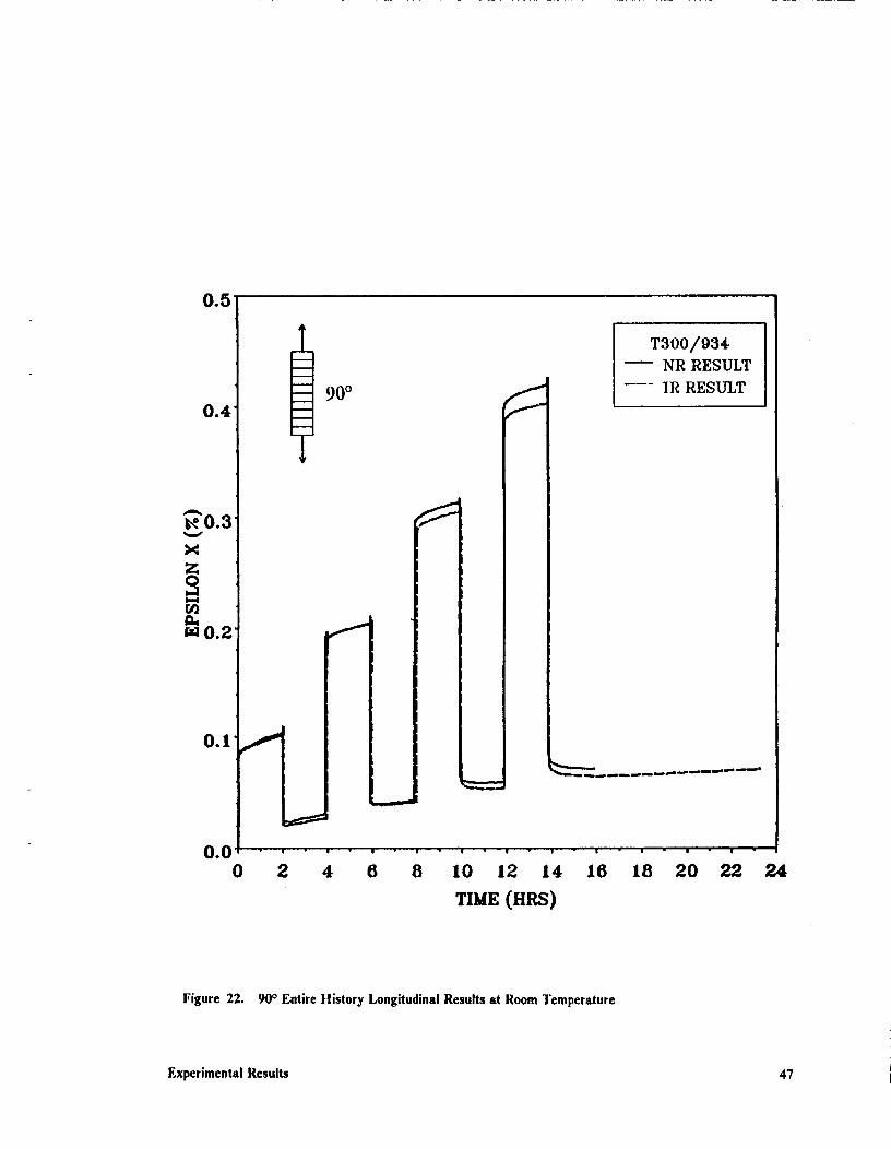
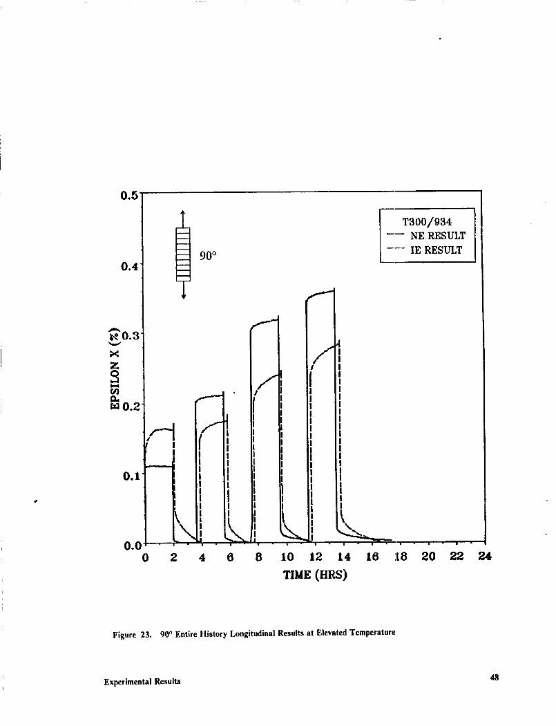
Figure 22 and Figure 23 show the longitudinal creep response for the entire loading history of the

90° tensile coupons. Figure 22 shows the room temperature results and Figure 23 shows the ele-

vated temperature results. As with the 10° tests, the room temperature results are nearly identical

for the two conditions. The load levels for both conditions are the same. Both specimens show

creep behavior at all load levels. The recovery, however, seems to proceed in a different manner

than observed with previous results. The recovery after the initial two loadings appears to be rep-

resentative of creep rather than recovery. This behavior will be discussed in Section 3.6.3.

The elevated temperature results show a difference but one not nearly as dramatic as for the 10°

results. The load levels for these two tests are not the same due to the much lower ultimate stress

of the IE specimen. The non-irradiated result is similar to the room temperature results. 'lhe

irradiated condition does exhibit significant creep but the difference between the IE and NE results


0.8'

0.7'

0.6'

0,2

10 °

T300/934

--- NR RESULT

--- IR RESULT

TIME (HRS)

Figure 20. 10 ° Entire History Shear Results at Room Temperature


0.71

0.6

AO.5

¢q

0.2

0.1

I0 °

/I,, /I!

/ I/ i I

I ! !I I II I I

f I i/i' I, a I i

' \ 1',,d

f

0.0 ' • "_"

0 2 4 6 8

/j/ ,

I

T300/934

NE RESULT

--- 1E RESULT

!

i -'1 . i - i - i - [ - | -

10 12 14 16 IB 20 22 24

TIME (HRS)

Figure 21. 10° Entire llistory Shear Results at Elevated Temperature


isn't nearly as great as the difference seen with the 10° tests. The recoveiy for both cases appears

to approach strain values lower than the initial strain. This will be discus:_ed in Section 3.6.3.

The state of stress in a 90° coupon subjected to uniaxial tension is composed of principal normal

stresses with little if any shear stress present. As seen in the 10° off-axis re:_ults, shear stresses in the

matrix appear to have a significant effect on the creep response of the spe:imen. The fact that the

creep response is diminished significantly when the shear stress is eliminated, such as with the 90°

tests, leads to the assumption that creep is most apparent in shear. While normal stresses do have

a significant effect on the creep response, this effect is not as great as seen when shear stresses in the

matrix are present.

3.4 Individual Results

To better see the effect of radiation and temperature on the creep response of both the T300/934

graphite/epoxy composite and the bulk 934 resin, individual results at a given load level for all

conditions will be presented. The results from all four conditions (NR,IF'.,NE,IE) are presented for

each test. Longitudinal (_x) and shear (y_) results are presented for the 10° and 45 ° off-axis tests

and longitudinal results alone are presented for the 90° and bulk resin tests. The creep and recovery

results are presented for a single loading and recovery at a given load level As mentioned in Section

2.5, each test consisted of four loadings at appro ximately 20%, 40 %, 60o/,,, and 80 % of the ultimate

load. Since the ultimate loads vary widely between differing conditions, each condition is not

loaded to the same load levels [161. For this reason, only two load levels are compared for each test.

For these results, the initial strain readings for each loading have been set to zero so that the creep

responses can be accurately compared. As shown in Section 3.3, permanent strains are often

present upon recovery. In the following plots, the permanent strain v_lues have been subtracted


0.5'

0.4

0.2"

90 °

f

TaOO/984

NR RESULT

--- ]R RESULT

O] L "--" _ _ ...............0 • | • l • l - I ! l ! l • l • I - i - l - i -

0 2 4 6 8 10 12 14 16 18 20 22 24

Tree

Figure 22. 90 ° Entire History Longitudinal Results at Room Temperature


0.5"

0.4'

A

t_ 0.3

Z

a,m 0.2

I

0.1

0.00

4,

.--L.i--.-.--i

i.....---I

90 °I,.--,,.---4

I--'-'-'1

I

f

ffIIIII

I II I

fI

f

T300/934---- NE RESULT

IE RESULT

f

|| . _ •

2 4 6 8 10 12

TIME (HRS)

Figure 23. 90 ° Entire History Longitudinal Results at Elevated Temperature


from the actual strain values so that each test is presented from the same initial strain value, namely

zero strain. This should be kept in mind when reviewing the following plots.

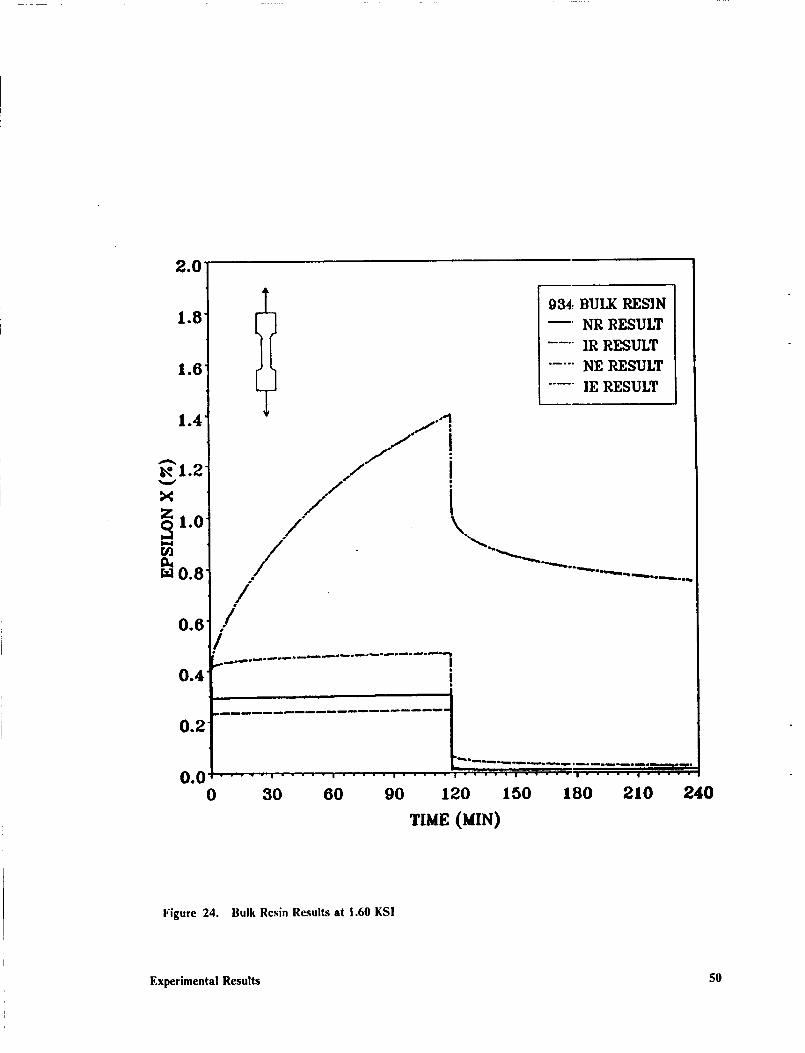
3.4.1 Bulk Resin Results

Figure 24 shows the creep response for the bulk resin results under a constant load of 1.60 KSI.

This is the initial loading for all conditions. The NR and IR results are nearly identical except for

the elastic response. The NE test does show a slight increase in the creep behavior while the IE test

shows a dramatic increase in the creep response. The recovery for the IE result shows a large per-

manent strain. The differences in the elastic response of these specimens correlates well with the

elastic moduli evaluated by Fox, et. at. 129]. A comparison of the elastic moduli is given in Ap-

pendix C.

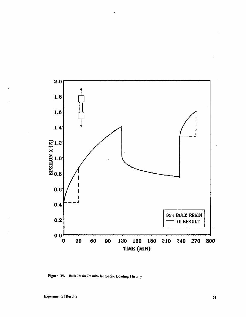
A second figure for the second load level is not shown since the strain on the initial loading for the

IE test nearly approached 2% and the gages only functioned properly up to this level. The gages

began to peel off soon after the second load level. Figure 25 shows the entire strain history of the

IE bulk resin test which only goes slightly beyond the second loading. As observed in the figure,

the creep after 30 minutes at the second loading is less than the creep after 30 minutes at the initial

loading. This agrees with the decrease in creep behavior on subsequent loadings seen with the

graphite/epoxy composite results.

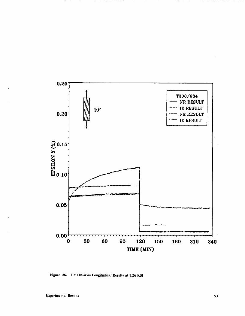
3.4.2 10 ° Results

Figure 26 shows the longitudinal creep response of the 10° off-axis tensile coupon under a constant

load of 7.26 KSI. This is the initial loading for all conditions. The NR and IR conditions are

nearly identical in the creep response. The NE creep response is slightly greater. The NR, IR, and


2.0

1.8

1.6

1.4

1.2

I,...4

0.8

0.6

0.4

0.2

[

[

//

//

///

.J'1/ I

// )/ I

984,- BULK RESIN

--" NR RESULT

.... IR RESULT

..... NE RESULT

.... IE RESULT

i

00. ..... '....................... " .... ' ..... ' .....0 30 60 90 120 150 180 210 240

TIME (MIN)

Figure 24. Bulk Resin Results at 1.60 KS!


0.2'

0.00

IIII

934 BULK RESIN

]E RESULT

..... I ..... I ..... I ..... I ..... e ..... | ..... | ..... I ..... I .....

30 60 90 120 150 180 210 240 270 300

TIME (MIN)

Figure 25. Bulk Resin Results for Entire Loading tlistory


NE results are all fairly similar and differ only in the magnitude of the elastic response. The IE

result is quite different from the other conditions. Significant creep is present in this condition and

the recovery exhibits a large permanent strain.

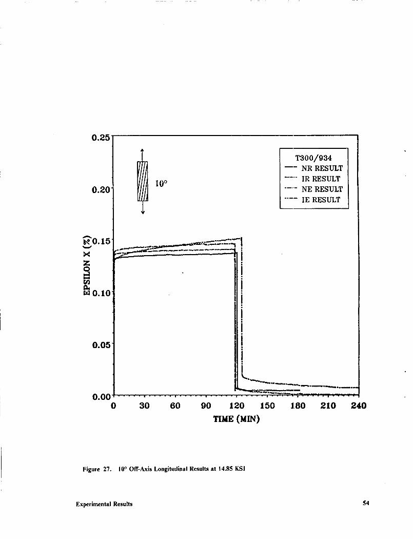
Figure 27 shows the longitudinal creep response for the 10° off-axis test under a constant load of

14.85 KSI. This is the second loading for the NR, IR, and NE results and the third loading for the

IE result. The creep response for the NR, IR, and NE results is simil_: to the results shown in

Figure 26 for 7.26 KSI while the 1E result is quite different from the IE response at 7.26 KSI. The

creep response is still greater for the IE condition as compared with the olher conditions but it isn't

nearly as significant as seen on the initial loading. The recovery at 14.85 KSI exhibits less perma-

nent strain than observed at 7.26 KSI. It should be noted that this is th_ third loading for the IE

test and the creep response seems to diminish with each successive loadir g.

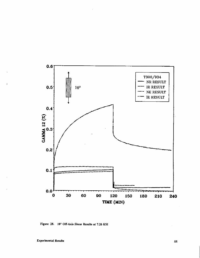
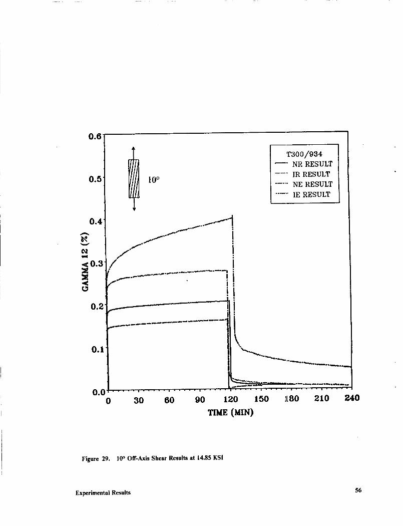
Figure 28 and Figure 29 show the 1-2 shear creep response in the material principal coordinate

system for the 10° off-axis tensile coupon under a constant load of 7.2,5 KSI and 14.85 KSI re-

spectively. Similar trends can be seen here as compared with the longitudinal creep response. The

magnitudes in shear, however, are much greater than the longitudinal strain magnitudes. For tile

IE results at 7.26 KSI, the creep in shear is very significant and the recovery exhibits a large per-

manent strain. At 14.85 KSI, the creep response for the IE condition diminishes somewhat and the

recovery shows less permanent strain. The important point to note here is the overall magnitude

of the creep response in shear.

3.4.3 45 ° Results

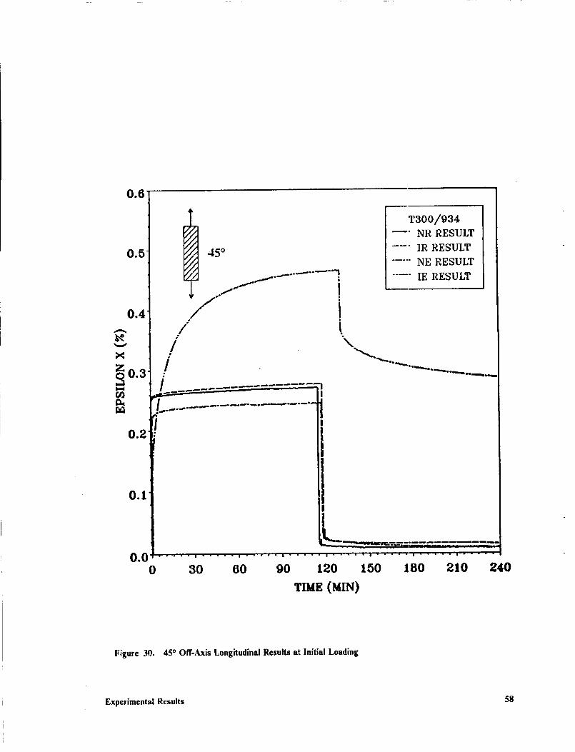
Figure 30 shows the longitudhaal creep response for the 45° off-axis teasile coupon at the initial

load level. Bccause of failure of many of the specimens at loads well betow the ultimate loads ob-

served by Milkovich, et al. [16], the initial load level for the NR, IR, and NE specimens was at 4.20


0.25

0.20

0.15

>¢

U2

_0.I0

0.05

0.000

10 °

T300/934

NR RESULT

--" |R RESULT

.... NE RESULT

"'-- ]E RESULT

w m mBw

.... ] -- m ___ -: I I_ J'

" " " " " I ..... I ..... I ..... II ..... ! ..... "l ..... I .....

30 60 90 120 150 180 210 240

TIME(MIN)

Figure 26. 10° Off-Axis Longitudinal Results at 7.26 KSI


0.25

0.20

_._0.15

i_0.I0

0.05

0.000

10 °

T300/934

m- NR RESULT

.... IR RESULT

.....NE RESULT

.... IE RESULT

IiI

.... ' - e .... • i ..... ! .....

30 60 90 120 150 180 210 240

TIME (MIN)

Figure 27. 10 ° Off-Axis Longitudinal Results at 14.85 KSI


0.6"

0.5

0.4

<0.3:Z:Z<

0.2

0.1

0.00

10 °

f----"!

// !/

//

/

I

I!\

T300/034

-- NR RESULT

--- )R RESULT

.... NE RESULT

"-- IE RESULT

i i i m ii I

h

L_wuN

,,, . , i n i n

..... u ..... I ..... ¢ ..... I ..... i ..... ! ..... I • - " _ -

30 60 90 120 150 180 210 24.0

TIME (MIN)

Figure 28. 10 ° Off-Axis Shear Results at 7.26 KS!


0.6"

0.5

0o4'

A

gq

<0.3

:Z

r_

0.2'

0.1

I0 °

/ t"''_'_ !/ I

I!

j_m _u l_wi_ _'_l_" _-w,_ _,_ j_ _ ,i

0.0 _

0 30 60 90

T300/934

--" NR RESULT

--" ]R RESULT

..... NE RESULT

.... IE RESULT

I\

120 150 JL80 210 240

TIME (MIN)

Figure 29. 10 ° Off-Axis Shear Results at 14.85 KS!


KSI and the initial load level for the IE condition was at 1.50 KSI. The plot is similar to the one

shown in Figure 26. The NR, IR results are fairly similar and the NE condition shows slightly

more creep than the room temperature results. The IE condition shows significantly more creep

and the recovery exhibits a large permanent strain. It should also be noted that the creep for the

IE condition does seem to level off quickly although the initial response is fairly steep.

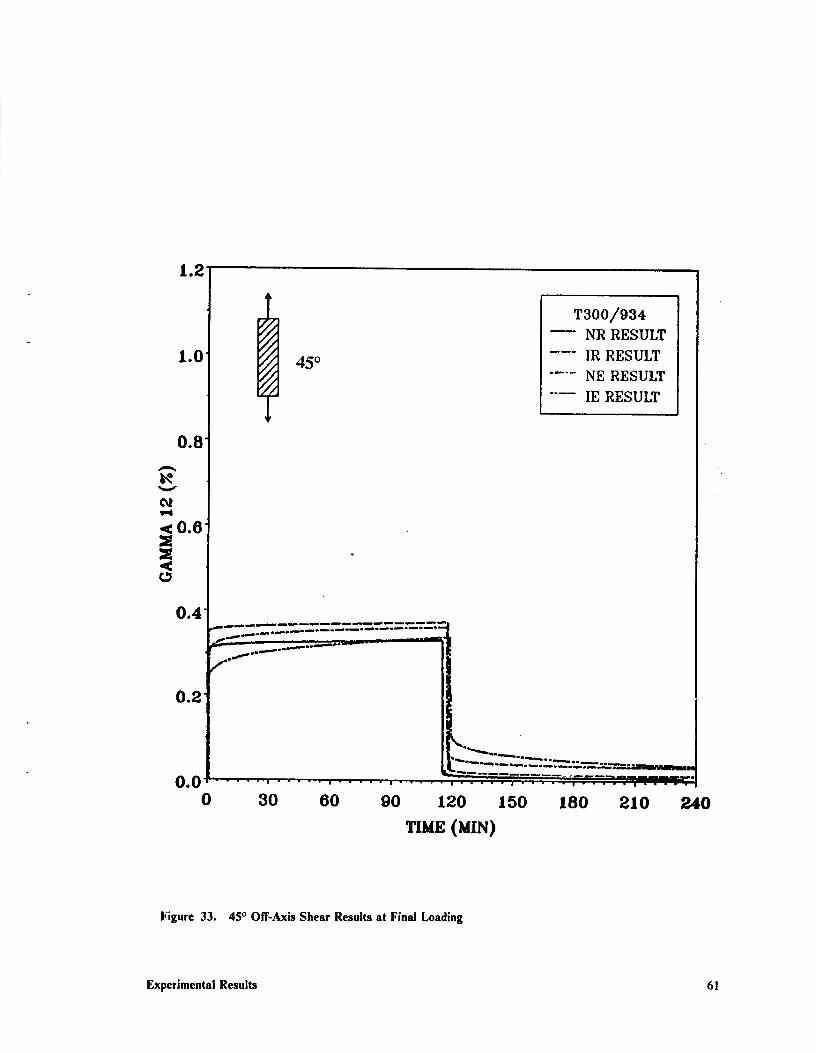
Figure 31 shows the longitudinal creep response for the 45 ° tensile coupon at the initial load level

of 4.20 KSI for the NR, IR, and NE tests and the final load level of 3.75 KSI for the IE test. The

NR, IR, and NE results are the same as in Figure 30 but the IE results are again quite different

compared to the IE response at 1.50 KSI shown in Figure 30. The creep response of the IE

specimen is very close to the response of the other conditions. It is slightly greater than the N R,

IR, and NE conditions but it is still much less than the IE creep response seen in Figure 30. The

recovery in this case exhibits little permanent strain.

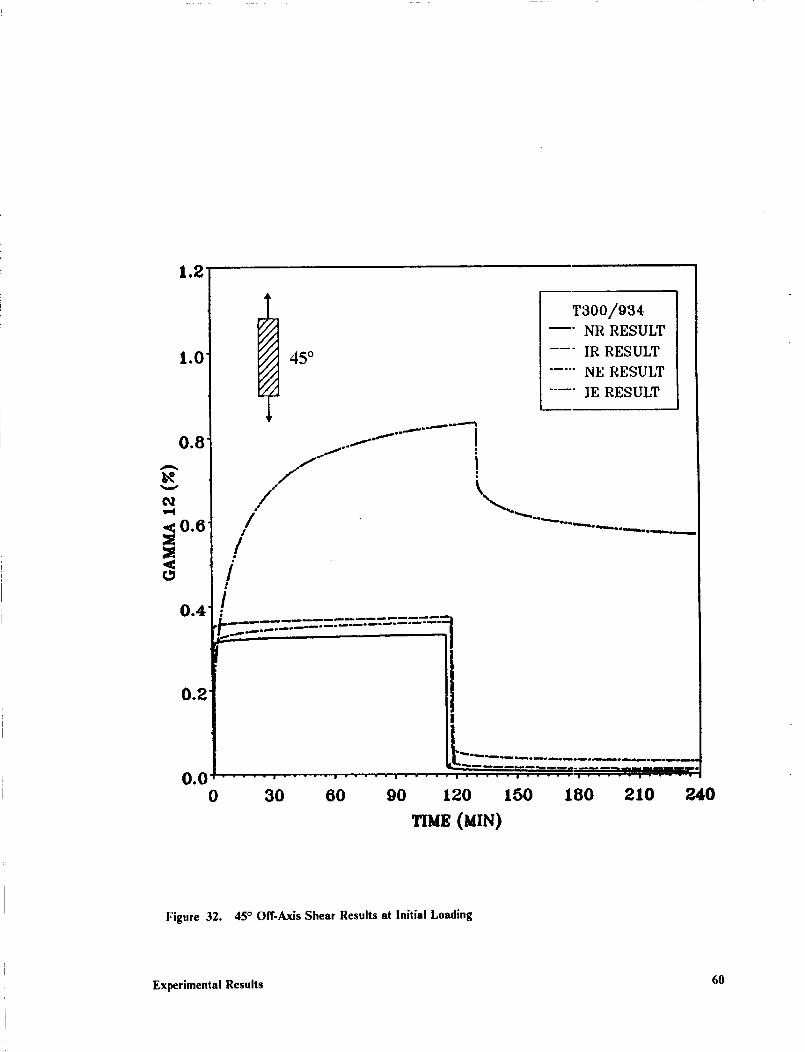
Figure 32 and Figure 33 show the shear creep response in the material principal coordinate system

for the 45° off-axis tensile coupon at the same loads as in Figure 30 and Figure 31. These plots

show similar trends. The NR, IR, and NE results are nearly identical except for the elastic re-

sponse. The IE creep response is significant on the first loading and is much less on the fmal

loading. The recovery exhibits a large permanent strain after the initial loading and little permanent

strain after the final loading. Again it should be noted that the magnitude of the creep response in

shear is significant when compared to the creep response in the longitudinal direction.

3.4.4 90 ° Results

Figure 34 shows the longitudinal creep response for the 90° tensile coupon at a constant load of

1.21 KSI. This is the initial load level for all conditions. The NR, IR, and NE results are similar

except for the elastic response. The NE result does show slightly more creep. The IE results shows


0.6"

0.5'

0.4

A

x

0.3

0.2

0.1

0.00

T300/934

--" NR RESULT

45 ° ---" IR RESULT..... NE RESULT

,._-""'_'" i IE RESULT

.I" [

// I/ t

/ ,,

• .... i ..... I ..... i ..... I ..... I ..... I ..... I .....

30 60 90 120 150 180 210 240

TIME (MIN)

Figure 30. 45 ° Off-Axis Longitudinal Results at Initial Loading


0.6

0.5

0.4 ¸

A

b-4

0.2"

0.!

45 °

T300/934

NR RESULT

--- ]R RESULT

.... NE RESULT

IE RESULT

o.o 0 30 60 90 120 150 180 2xo _0

TIME(MIN)

Figure 31. 45 ° Off-Axis Longitudinal Results at Final Loading


1o2 _

1.0

0.8

A

t'q

<0.6

0.4'

0.2

0.00

45 °

T300/934

-- NR RESULT

]R RESULT

..... NE RESULT

IE RESULT

/..I !J

//

!

//

!

/

30 60 90

_' 'gmmm_,mmm_ Q11_mmt_ mqmlfm.q_l,_ _

120 150 180 210 240

TIME (MIN)

Figure 32. 45 ° Off-Axis Shear Results at Initial Loading


1.2'

1.0'

0.8"

A

¢q

,<0.6

0.4

45 °

T300/934

NR RESULT

--- IR RESULT

.... NE RESULT

"'-- IE RESULT

0.0 .............

0 30 60 90 120 150 180 210 P,40

TIME (MIN)

Figure 33. 45 ° Off-Axis Shear Results at Final Loading


more creep than the other conditions but not to the extent seen in the off.axis tests. The recovery

for the IE and NE results appears to be approaching a final state below zeio strain. It actually does

proceed below zero before the test is completed. This will be discussed in Section 3.6.3. The NR

and IR recovery results appear to be in error since the strain is increasing rather than decreasing.

This will also be discussed in Section 3.6.3.

Figure 35 shows the longitudinal creep response for the 90° tensile coupon at a constant load level

of 2.42 KSI. This is the second loading for the NR, IR, and NE tests and the third loading for the

IE test. The creep response for the NR, IR, and NE results is again similar and here the IE creep

response more nearly approaches the response of the other conditions. The IE response is still

greater at 2.42 KSI but not as much as seen at 1.21 KSI. The recovery again seems to be headed

below zero for the elevated temperature results and in fact does go below zero before the test is

completed.

3.5 Linearity

In Chapter 4.0, it is assumed that the material used in this study behave:_ as a linearly viscoelastic

material. The conditions and importance of linearity will be discussed irt that chapter. An exper-

imental method to check for linearity will be employed in tiffs section for both the bulk resin and

composite results.

3.5.1 Linearity Verification

A commonly used method to determine linearity of a material is to cor.struct isochronous stress-

strain curves where stress and strain values are plotted for a constant time value. As an example,


0.40"

TSOO/g840.35 _ NR RESULT

900 --" IR RESULT.... NE RESULT

0.30 "'-- IE RESULT

0.20

o.15!.-f" !

i.................... 41 i

L005t i_. I

I I .... "-"-,...,..,. ...... I0.00 k..,..

_0.25

0 30 60 90 120 150 180 210 240

TIUE(uzN)

Figure 34. 90° Longitudinal Results at 1.21 KSI


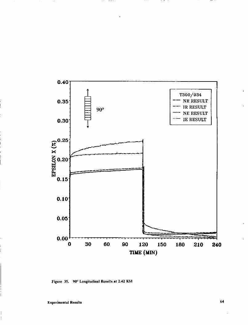
0.40

0.35

0.30

X

0.20

r,_0.15"

0.10

0.05

90 °

Ta00/9a4

_m NR RESULT

IR RESULT

..... NE RESULT

.... IE RESULT

1..,,.._..,.._....... ---""""" _ .--.

o.oo _ -"_--0 30 60 90 120 150 180 210 240

Tree (raN)

Figure 35. 90° Longitudinal Results at 2.42 KS!


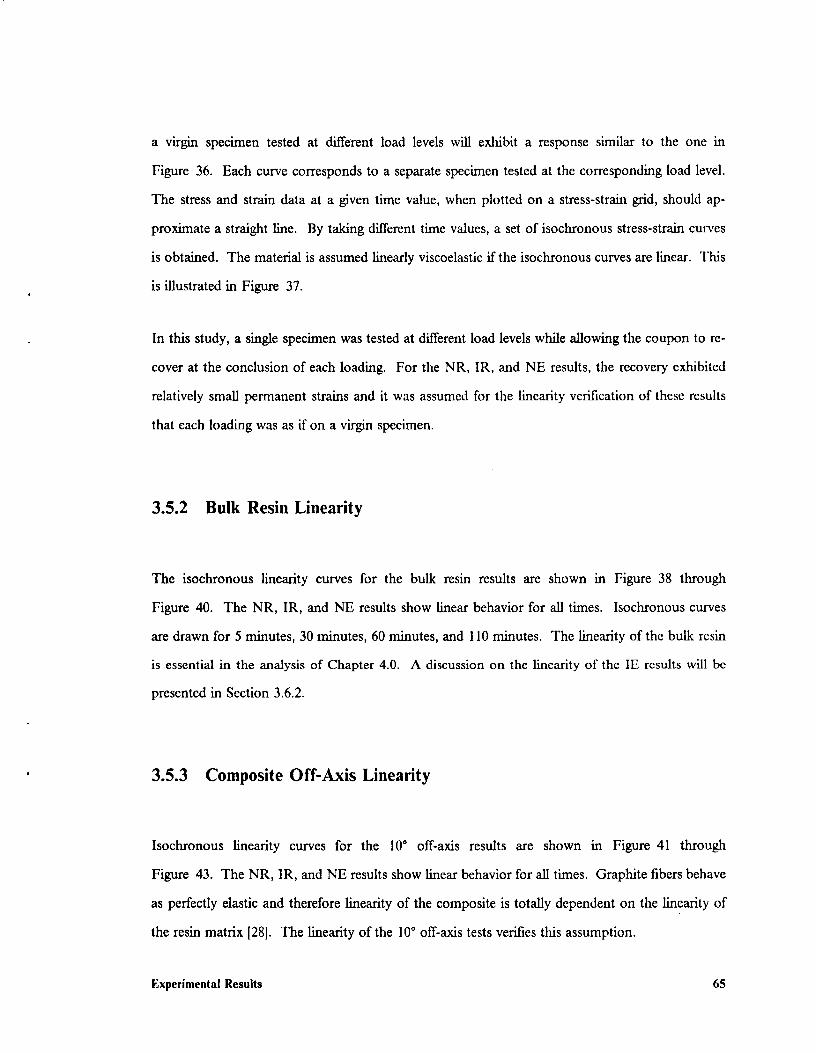
a virgin specimen tested at different load levels will exlfibit a response shnilar to the one in

Figure 36. Each curve corresponds to a separate specimen tested at the corresponding load level.

The stress and strain data at a given time value, when plotted on a stress-strain grid, should ap-

proximate a straight line. By taking different time values, a set of isochronous stress-strain curves

is obtained. The material is assumed linearly viscoelastic if the isochronous curves are linear. This

is illustrated in Figure 37.

In this study, a single specimen was tested at different load levels while allowing the coupon to re-

cover at the conclusion of each loading. For the NR, IR, and NE results, the recovery exhibited

relatively small permanent strains and it was assumed for the linearity verification of these results

that each loading was as if on a virgin specimen.

3.5.2 Bulk Resin Linearity

The isochronous linearity curves for the bulk resin results are shown in Figure 38 through

Figure 40. The NR, IR, and NE results show linear behavior for all times. Isochronous curves

are drawn for 5 minutes, 30 minutes, 60 minutes, and 110 minutes. The linearity of the bulk resin

is essential in the analysis of Chapter 4.0. A discussion on the linearity of the IE results will be

presented in Section 3.6.2.

3.5.3 Composite Off-Axis Linearity

Isochronous linearity curves for the I0 ° off-axis results are shown in Figure 41 through

Figure 43. The NR, IR, and NE results show linear behavior for all times. Graphite fibers behave

as perfectly elastic and therefore linearity of the composite is totally dependent on the linearity of

the resin matrix [28]. The linearity of the 10° off-axis tests verifies tiffs assumption.


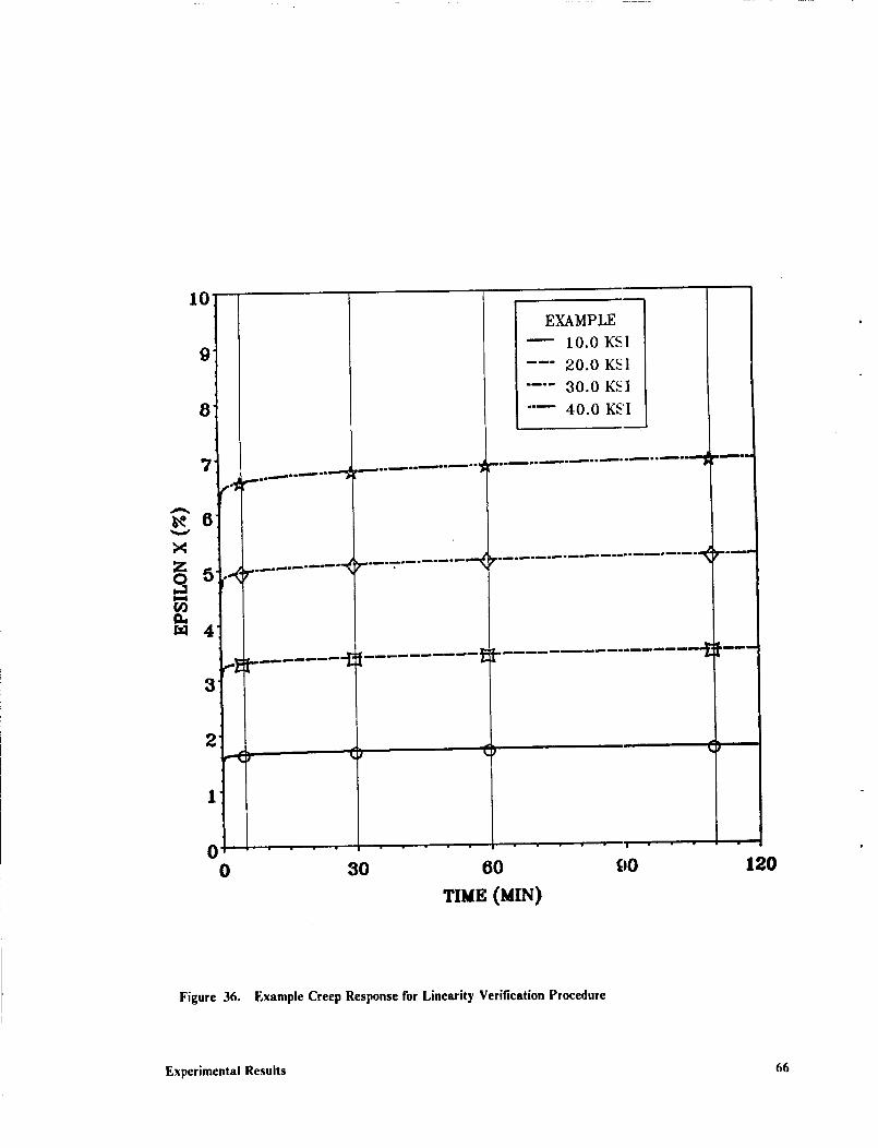
10

,

8

EXAMPLE

-- 10.0 KSI

--" 20.0 KSI

.... 30.0 KSI

"'-- 40.0 KSI

7,_,_ ........ ---_

A

6

p_ _._mam_mamul_m" _

z r .......... "<r'-'- ........ "-(_

,

_aml_

k"'d

,

1

,-<, () () (,

00 30 60 90

TIME (MIN)

120

Figure 36. Example Creep Response for Linearity Verification Procedure


5O

4O

10

4 5 6

EPSILOr_ X (_.)

EXAMPLE

o _ T- 5 MIN

n --- T= 30MIN

¢ .... T= 60 MIN

"'_ T= if0 MIN

7 8 9 10

Figure 37. Example Isochronous Lines for Linearity Verification Procedure


8

,

6

3

2 234 BUIX RESIN

o ---- T= 5 MIN

'_ .... T= 30 MIN

i¢ ..... T= 60 MIN

_ .... T-- II0 MIN

00.0 0.2 0.4 0.6 1.2 1.4 1.6 1.8

Figure 38. NR Bulk Resin Linearity Verification


8

7

6

2

1

00.0

- - - I " " " I " " | • • - I " " " I

0.2 0.4 0.6 0.8 1.0

EPSILON X (7_)

g84 BULK RESIN

o _ T= 5 MIN

n --- T= 30MIN

¢ .... T= 60 MIN

"'-- T= 110 MIN

| - • | - • - I " "

1.2 1.4 1.6 1.8

Figure 39. IR Bulk Resin l.inearity Verification


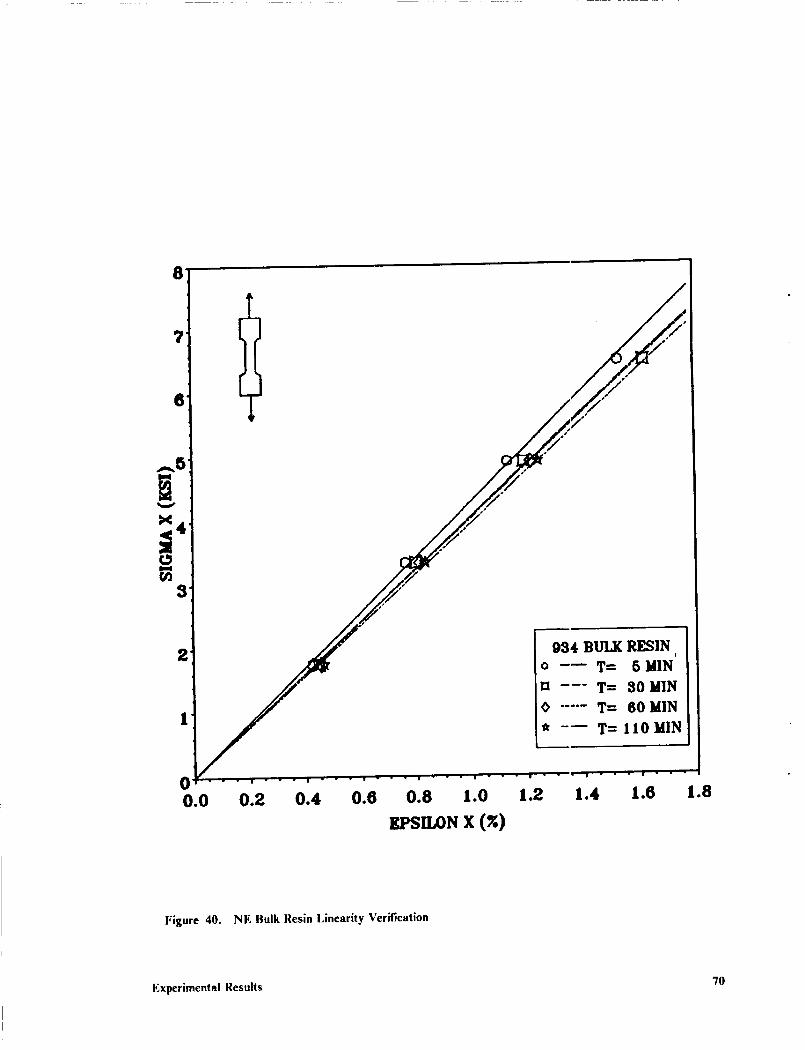
8

2 934 BULK RESIN}

o -_ T= 6 MIN

n --- T= 30MIN

¢ ..... T= 60 MIN

_r ---- T= I10MIN

00.0 0.2 0.4 0.6 1.2 1.4 1.6 1.8

Figure 40. NE Bulk Resin Lincarity Verification


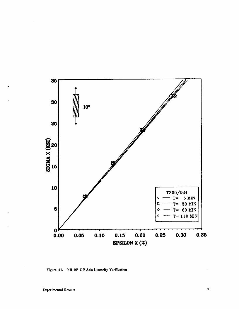
35

30

25

15

10

5

T300/934o _ T= 5 MIN

--- T= 3O MIN

0 .... T= 60 MIN

¢r T= ItO MIN

00.00 0.05 0.10 0.15 0.20

IzPSILON X (%)

0.25 0.30 0.35

Figure 41. NR 10 ° Off-Axis I,inearity Verification


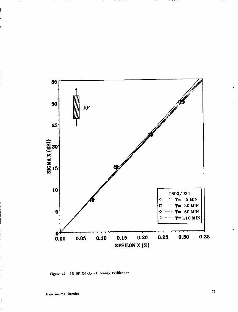
25

10°

I0

5

T300/934o --- T= 5 MIN

.... T= 30 MIN

.... T= 60 MIN

_' .... T= It0 MIN

00.00 0.05 O.lO 0.15 0.20

EPSILON X (7.)

0.25 0.30 0.35

Figure 42. IR 10 ° Off-Axis Linearity Verification


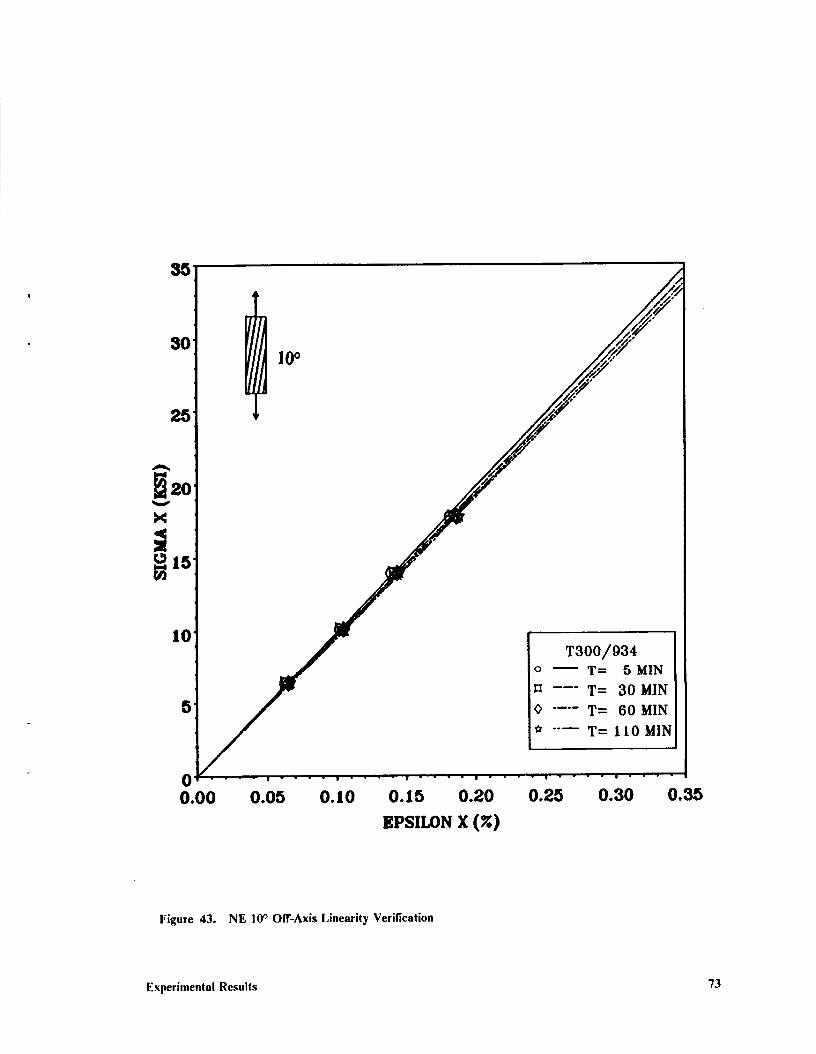
l0 °

00.00 0.05 0.10 0.15 0.20

EPSILON X (7.)

T300/934

o _ T= 5 MIN

la T= 30 MIN

<> .... T= 60 MIN

..m T= IL0 MIN

0.25 0.30 0.35

Figure 43. NE l0 n Off-Axis Linearity Verification


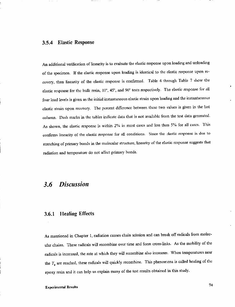
3.5.4 Elastic Response

An additional verification of linearity is to evaluate the elastic response upon loading and unloading

of the specimen. If the elastic response upon loading is identical to the elastic response upon re-

covery, then linearity of the elastic response is confLrmed. Table 4 through Table 7 show the

elastic response for the bulk resin, 10°, 45°, and 90° tests respectively. The elastic response for all

four load levels is given as the initial instantaneous elastic strain upon loading and the instantaneous

elastic strain upon recovery. The percent difference between these two values is given in the last

column. Dash marks in the tables indicate data that is not available frown the test data generated.

As shown, the elastic response is within 2% in most cases and less than 5% for all cases. This

confirms linearity of the elastic response for all conditions. Since the _lastic response is due to

stretching of primary bonds in the molecular structure, linearity of the elastic response suggests that

radiation and temperature do not affect primary bonds.

3.6 Discussion

3.6.1 Healing Effects

As mentioned in Chapter 1, radiation causes chain scission and can break off radicals from molec-

ular chains. These radicals will recombine over time and form cross-links. As the mobility of the

radicals is increased, the rate at which they will recombine also increase.';. When temperatures near

the Ts are reached, these radicals will quickly recombine. This phenorr_ena is called healing of the

epoxy resin and it can help us explain many of the test results obtained in this study.


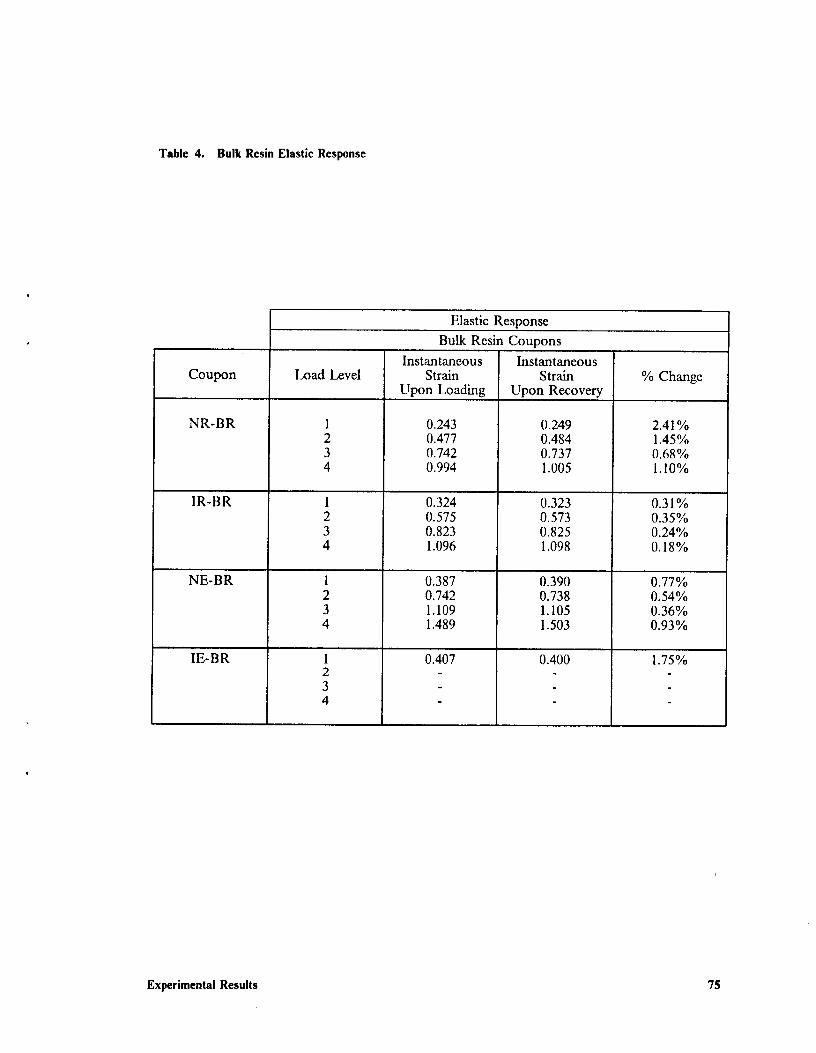
Table 4. Bulk Resin Elastic Response

Elastic Response

Bulk Resin Coupons

Instantaneous InstantaneousCoupon Load Level Strain Strain % Change

Upon Loading Upon Recovery

NR-BR

IR-BR

NE-BR

IE-BR

1234

1234

0.2430.4770.7420.994

0.3240.5750.8231.096

0.3870.7421.1091.489

0.407

0.2490.4840.7371.005

0.3230.5730.8251.098

0.3900.7381.1051.503

0.400

2.41%1.45%0.68%1.10%

0.31%0.35%0.24%0.18%

0.77%O.54%0.36%0.93%

1.75%


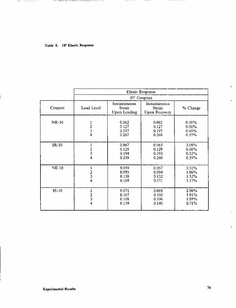
Table 5. 10° Elastic Response

Elastic Response

10° Coupons

Instantaneous InstantaneotLs

Coupon Load Level Strain Strain % ChangeUpon Loading Upon Recow,,ry

NR-10

1R-IO

NE-10

IE-10

1234

1234

1234

0.0620.1270.1970.267

0.067O. 129O. 1940.259

0.0590.0950.1300.169

0.0710.1070.1080.139

0.0620.1270.1970.268

0.0650.1290.1930.260

0.0570.0940.1320.171

0.0690.1050.1060.140

0.00%0.00%0.00%0.37%

3.08%0.00%0.52%0.39%

3.51%1.06%1.52%1.17%

2.90%1.91%1.89%0.71%


Table 6. 45 ° Elastic Response

Elastic Response

45" Coupons

Instantaneous Instantaneous

Coupon Load Level Strain Strain % ChangeUpon Loading Upon Recovery

NR-45

IR-45

NE-45

IE-45

1234

1234

1234

1234

0.2580.3690.477

0.2520.347

0.2240.3510.412

0.1000.1210.1470.169

0.2610.372

0.488

0.248

0.348

0.2170.3530.403

0.0960.1200.1400.160

1.15%0.81%2.25%

1.61%0.29%

3.23%0.57%2.23%

4.17%0.83%5.00%5.63%


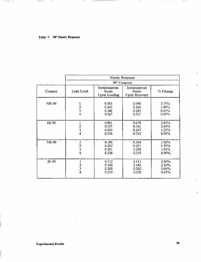
Table 7. 90° Elastic Response

Elastic Response

90° Coupons

Instantaneous InstantaneousCoupon Load Level Strain Strain % Change

Upon Loadhag Upon Recovery.

NR-90

IR-90

NE-90

IE-90

1234

1234

0.0830.1630.2460.327

0.0810.1570.2500.336

0.1060.2020.3010.338

0.1120.1400.2000.235

0.0800.1600.2450.327

0.0780.1610.2470.333

O.1040.2010.2980.335

0.1110.1430.2020.236

3.75%1.88%0.41%0.00%

3.85%2.48%1.22%0.90%

1.92%0.50%1.01%0.90%

0.90%2.10%1.00%0.42%


TheIE resultsinall casesseemto bearout thishealingeffect.Asshown,thefirstloadingalways

exhibitedthegreatestcreepbehaviorwhilesubsequentloadingsexhibiteda relativedecreasein the

creepbehavior.Additionally,therecoverydatashowslargepermanentstrains.At + 250 °F, the

broken chains in the epoxy are quite mobile and will slide, twist, and uncurl rapidly. Also at this

temperature, radiation induced radicals in the epoxy are quite mobile and begin to recombine. As

the specimen is strained, the radicals are moved and form new cross-links in the strained condition.

Cross-linking in this fashion is an on-going process. Upon recovery, the epoxy is in a different state

than when the load was applied. In this state, more cross-links now exist, many of which were

formed in the strained state. This would create apparent permanent strain in the specimen. Upon

subsequent loadings, the structure is more cross-linked, more rigid, and more resistant to creep.

This would explain the decrease ha creep behavior and the decrease in permanent strains seen upon

subsequent loadings.

To verify this healing effect, some additional tests were run. Since cross-links are continually being

reformed in the IE condition, some irradiated 10° specimens were tested after being pre-soaked at

+ 250 OF for varying amounts of time. Figure 44 shows the creep response of these tests. As

shown, the longer the specimen is exposed to + 250 °F, the less creep behavior is seen. After eight

hours at + 250 OF, the creep response of the 10° off-axis specimen is approaching the NR creep

response of the material. This suggests that healing is taking place while the temperature is held

at + 250 °F.

The linearity of the elastic response for the IE condition coupled with the healing of the time-

dependent response suggests that radiation is only affecting secondary bonds of the epoxy network.

It also suggests that the healing process is only concerned with secondary bonds and does not affect

the primary bonds of the structure. Upon loading, the stretching of primary bonds is instantaneous

and is evidenced in the elastic response of a test specimen. Twisting, uncurling, and sliding of sec-

ondary bonds is time-dependent and is evidenced in the viscoelastic response of a test specimen.

Radiation and healing seem to affect only the viscoelastic response of the tested specimens and not

the elastic response.


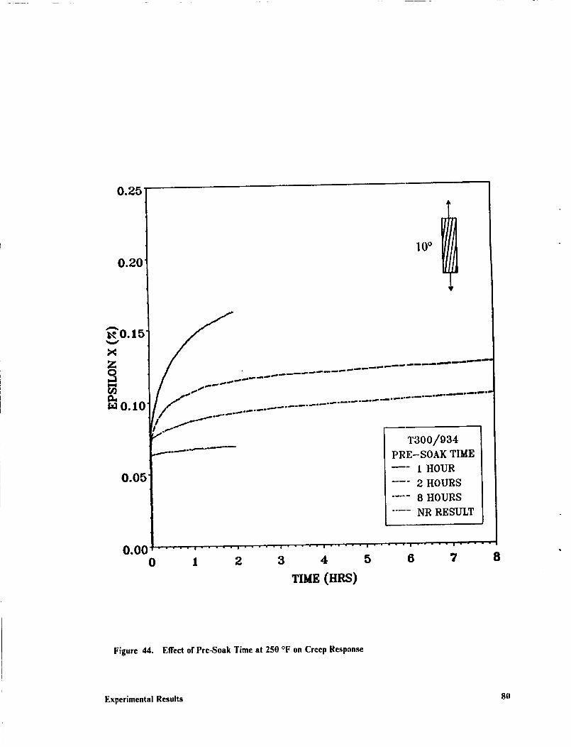
0.25

0.2010°

0.15] _i"

t/ ___-................II ./---"

1_ // ..._ __.............m O 1011 .f ........................

.... Jl/ ..............

0.05

T300/934

PRE-SOAK TIME

--- l HOUR

-- 2 HOURS

.... 8 HOURS

.... NR RESULT

1 2 3 4 5 6 7 80.00

0

TIME (HRS)

Figure 44. Effect of Pre-Soak Time at 250 °F on Creep Response


3.6.2 IE Linearity

Because of the healing process, the evaluation of linearity in the IE bulk resin is a complicated task.

Viscoelastic linearity, as it has been assumed in this study, is dependent on stress, strain, and time.

The healing process appears to be dependent on temperature and pre-soak time, both of which are

parameters not commonly associated with linear viscoelasticity. These additional parameters in-

troduce apparent nonlinearities into both the IE bulk resin response and the IE composite response.

The healing process constantly changes the state of the material. Since viscoelastic linearity is a

material property, as the material changes through healing, so does the linearity of the material.

This manifests itself as apparent nonlinearity of the material. Although the IE material may be

linear at any given time, linearity in the general sense cannot be assumed for this condition.

3.6.3 90 ° Recovery Discussion

"I'300/934 graphite epoxy is a + 350 °F cure epoxy system. Upon curing, cross-linking occurs at

+ 350 °F to make the epoxy a rigid structure. Upon cooling, the epoxy ha an unconstrained state

contracts isotropically while the unconstrained graplfite fibers expand slightly in the longitudinal

direction. Because of constraints present in the composite, tensile residual stresses in the fiber di-

rection are present in the matrix and compressive residual stresses in the fiber direction ,are present

in the fibers. The residual stresses in the fiber and matrix increase as the graphite/epoxy composite

is cooled from + 350 °F. In other words, the residual stresses in the composite at room temperature

would be greater than the residual stresses at + 250 °F. This phenomena may explain the differ-

ences in the recovery responses of the 90° room temperature coupons and the 90° elevated tem-

perature coupons.

Tensile residual stresses in the fiber direction that are present in the room temperature

graplfite/epoxy material can be quite significant. A typical graphite/epoxy composite may have


tensile residual stresses in the matrix as high as 80-90% of the ultimate strength of the epoxy resin

[34]. Upon applying a tensile load to a 90° specimen, fibers and matrix contract transversely in

accordance with the composite Poisson's response. Under uniaxial loading, the unconstrained

matrix would contract more than a transversely loaded, unconstrained graphite fiber. Due to con-

straints in the composite, however, tensile residual stresses in the matrix in the fiber direction are

further increased. In a room temperature composite, this increases the ;_eady significant tensile

residual stresses in the matrix which may then become high enough to cause damage in the epoxy.

Damage would restrict the recovery of the coupon.

At + 250 °F, tensile residual stresses in the fiber direction that are present in the matrix would be

quite small. These tensile residual stresses in the matrix at + 250 °F will be on the order of only

20-30% of the ultimate strength of the epoxy resin [34]. Applying a tensile load to a 90° specimen

would create a tensile load in the matrix in the fiber direction. Since tensile residual stresses in the

matrix are minimal to begin with, residual stresses caused by uniaxial loading would not be signif-

icant enough to cause damage and the epoxy would creep in the direction of tim tensile residual

stress. Any permanent straha resulting from the creep of the epoxy woul d manifest itself in an in-

creased width of the specimen. An increased width of the specimen would create a decreased length

in accordance with the Poisson's response. This can explain the recovery dipping below zero for

the elevated temperature results.


4.0 Analytical Model

This chapter will discuss the formulation of the analytical prediction tool developed in this study.

The goal of the analytical formulation was to modify existing rnicromechanical models, now for-

mulated to predict elastic response, to have the capability to predict viscoelastic response as well.

This modification is accomplished by use of the Correspondence Principle.

A discussion of linear viscoelasticity and the principles behind it will first be presented along with

a discussion of the Correspondence Principle and its application to problems in linear

viscoelasticity. The micromechanics models will then be presented and discussed in addition to

how the Correspondence Principle can be applied to these models. A discussion will follow on the

viscoelastic modeling of the matrix and how the various viscoelastic parameters to be used with the

model formulation were evaluated. This chapter will end with a presentation and discussion of

sample results obtained from this predictive model formulation for glass reinforced epoxy.

Analytical Model 83

4.1 Linear Viscoelasticity

For a perfectly elastic material, the stress and strain is related by Hooke's I,aw. This law states that

°ij = Eukt ekt (4.1)

or,

_U= Do'kl °kt (4.2)

where o Uand eq represent the stress and strain respectively. E_j,t is known as the elasticity tensor

and Di_k_is known as the compliance tensor. A perfectly elastic material i,';characterized by stresses

and strains that are not dependent on time.

The response of a viscoelastic material is not only dependent on the present state of body forces

and surface tractions, but also on the entire history of such forces. Linear viscoelasticity is con-

cemed with materials whose time-dependent displacements and strains ar,_ small and can be super-

imposed in time according to the Boltzmann superposition principle. Assuming a homogeneous

material and a stress and strain field that are not space dependent, the Boltzmann superposition

principle states that

or,

t , dekl,_u(O= cukt (t - _ dr (4.3)lO0

ft , dokl_ij(t) = Sifta (t - "0--_-r d'r (4.4)--OO

Analytical Model 84

where the Cij,i (t) and So, I (t) are response functions which define the given material behavior. Tile

C0,/ (t) are known as the relaxation moduli and the S_,k_(t) arc known as the creep compliances.

The same symmetry conditions hold for these tensors as for the corresponding elastic tensors. In

order to determine these functions, we proceed in the following fashion. First define a step function

strain such that

where

ru(t) = e_jH(t) (4.5)

H(t)={i t>0t<0(4.6)

is defined as the unit step function.

The derivative of I l(t) is the delta function 6(0 defined as

6(0={01 Itlt_0>0 (4.7)

Inserting (4.5) into (4.3) gives

all (t) = Cijkt (t) ,°kt (4.8)

Similarly, imposing a step function stress

a ij ( t) = a_j tt (t) (4.9)

results in

rlj (0 = SIJkl ( t) a°kt (4.10)

Analytical Model 85

Equations (4.8) and (4.10) provide a convenient experimental method to determine G/kl(t) and

S0k/ (t). To determine the creep compliance S_j_I(t), for exanaple, a step function stress is applied.

By monitoring the strain % (t) as a function of time and dividing through by the stress level a]_, the

creep compliance S_jk_(t) is evaluated. A similar procedure is followed in evaluating the relaxation

moduli C,j,, (t) .

In the laboratory, measurements can only be made when the experiment begins, which leads to the

assumption

0 t<0_U( - oo, t) =e/j (t) t _>0

(4.11)

This expression contains a discontinuity at t = 0 which gives

_U( - oo, t) = _ij (0) H(t) + d U(t) (4.12)

where Gj is continuous and vanishes for t < 0. The derivative of the strain is therefore

d_U ddq (4.13)dt = qj (0)6(0 + d-"_

Inserting this into (4.3) we get

Io" " d_klolj (t) = Gila (t) ekl (0) + Gila (t -- "c)--d-_-_ d_+

(4.14)

Taking the same approach with a suddenly applied stress gives

" " dam Jeli (t) = Sqla (t) a1¢! (0) + Sidkt (t -- z)----_r av+

(4.15)

Equations (4.14) and (4.15) can be simplified by writing

Analytical Model86

"u (0 = f_c'ok_ (t - _) d_k_&&(4.16)

IO_ dO klelj (t) = So.kl (t -- -r)---_ dr

assuming that these integral expressions take jump discontinuities into account.

(4.17)

4.2 Correspondence Prhtciple

4.2.1 Laplace Transform Conversion

The Laplace transform is a useful tool in the field of viscoelasticity. The Laplace transform of a

function _b(t) is defined as:

OO•g'Ed,(t)] = _ (s) = e-st dp(t)dt"o

(4.18)

The convolution theorem is also useful here. The convolution of the Laplace transform is

._If ;_b(t- T)_b(r)dr] = qb(s)if(s) (4.19)

The Laplace Transform of a derivative is

._ = s 4, (s) - 4(0) (4.20)

Analytical Model 87

Using these expressions with 4_(0)= 0 and taking equations (4.16) and (4.17) and the Laplace

transforms of each gives

(s) = s cSjkt(s) _kt(s) (4.2l)

(s) = s SukI (s) _kt (s)

It can be seen from relations (4.21) and (4.22) that if it is allowed that

(4.22)

s Gjkt (s) = Fljkl (s) (4.23)

s _jkt (s) = Kljkl (s) (4.24)

then

_t) (s) = FUkt (s) gkt (s) (4.25)

_ij (s) = KUkt (s) -6kt(s) (4.26)

These equations are similar to an elastic stress-strain law. I"qk ! (S) and Kq_l (s) are known as the

transform domain moduli and compliances respectively.

4.2.2 Boundary Value Problems

Now consider a viscoelastic body in the presence of body tbrces.

equilibrium equations are

all j (x, t) = 0

Ignoring the inertia terms, the

(4.27)

To obtain the differential equations for the displacements, substitute (4.16) into (4.27) to get

Analytical Model 88

o2 rf' 0_(_,,) 7o_Lj °cukt(t-r) or drj=0 (4.28)

The boundary conditions on the surface S can be of tile type

ul (S,t) = u# on Su (4.29)

Tt (S,t) = Tit on S T (4.30)

where Su denotes the part of the surface over which the displacements are prescribed and Sr denotes

the part of the surface over which the tractions are prescribed. If the body is heterogeneous then

(4.29) and (4.30) must be satisfied in each phase and the additional boundary interface conditions

u_(_x,t)_ continuous on Sinterfacer_(x, t))

(4.31)

will be hnposed where S,,,,,I,co denotes all interface boundaries.

This boundary value problem is quite complicated in the space-time domain. If, however, tile

transforms of equations (4.28) through (4.31) are taken to the Laplace trzmsform domain, the

problem becomes

s Cokt uk,0 = 0 (4.32)

F (S,s) = _ on S u (4.33)

(S,s) = _ii on S T (4.34)

(x, s)}_ continuous on S_nterfaceTl (x, s)

(4.35)

where

Analytical Model 89

= s Gjkl uk,t nj (4.36)

Examination of equations (4.32) through (4.36) shows that these equations are analogous to a for-

mulation of an elasticity problem if the transform domain moduli s C,jk_= F_j,_ assume the role of

the elastic moduli. A convenient method of solving linear quasi-static viscoelastic problems,

therefore, is to solve the associated elastic problem, substitute in the transform domain moduli for

the elastic moduli, and obtain the transforms _,(_x,s) and _o(_, s) of the viscoelastic solution. In-

version of the Laplace transform then gives the viscoelastic solution. This is known as the Corre-

spondence Principle [35].

4.3 Microntechanical Models

Since the advent of composite materials, scientists and engineers have attempted to develop effective

methods for predicting their properties. Since composites are generally composed of two separate

materials whose material properties are known, it seems advantageous to develop models to predict

properties of the composite using the properties of the individual constituents. This would allow

the designer to look at many different combinations of materials to fred the one that best meets his

needs. The study dealing with this subject is that of micromechanics. The basic goal of micro-

mechanics is to model a "representative cell" consisting of, in the case of continuous fiber reinforced

composites, a single fiber and the surrounding matrix material. The objective is to analyze the

representative cell with the implication that this cell is "representative" of the total composite.

Micromechanics can not only be useful as a predictive tool but can also help us understand com-

posites at the "micro" scale of a single fiber.

Two micromechanical models that are being used today will now be discussed. The Composite

Cylinder Assemblage (CCA) model proposed by Hashin [36] will first be discussed. The Composite

Analytical Model 90

CylinderAssemblagemodeliswidelyacceptedin the field today. A relatively new model proposed

by Aboudi 1371will "also be discussed.

4.3.1 Hashin Model

Hashin [36] developed a rnicromechanical model called the Composite Cylinder Assemblage (CCA)

model. This model assumes that the composite can be modeled as a single cylindrical fiber sur-

rounded by a matrix sleeve. This is shown in Figure 45. The fiber volume fraction is used in this

model to calculate the ratio of the fiber radius to the matrix sleeve radius. Different sizes of these

composite-matrix cylinders with the same radii ratios can be assembled to fill up the free space and

model the total composite. Figure 46 shows the composite cylinder assemblage.

If we make these assumptions, the problem of determining the properties of a continuous fiber re-

inforced material reduces to that of solving the much simpler problem of a single composite cylinder

as shown in Figure 45. The single composite cylinder with the given radii ratio is considered a

representative cell. This turns out to be a fairly simple boundary value problem. The details of this

problem along with the solutions can be found in I-tashin 1361.

This boundary value problem can give us exact solutions of the model for the longitudinal Young's

modulus (Ell), the Poisson's response (El2), and the axial shear modulus (Gi2). Due to the geometry

of the composite cylinder, however, exact solutions of the model for the transverse properties of the

composite cannot be formulated. As a result, the Hashin model resorts to energy methods to give

upper and lower bounds for the transverse Young's modulus (E22), and the transverse shear

modulus (G23). In order to completely characterize a transversely isotropic composite, all five

properties must be evaluated.

Analytical Model 91

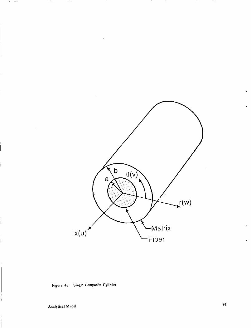
b

r(w)

x(u)vlatrix

Fiber

Figure 45. Single Composite Cylinder

Analytical Model 92

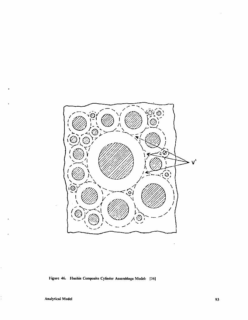
:,®),,-_-,', _/////_/g i¢'_T"

_hi \ wyi.pTII/l a_

Figure 46. Hashin Composite Cylinder Assemblage Model: [361

Analytical Model

93

4.3.2 Aboudi Model

The Aboudi [37] model is based on a repeating unit cell consisting of a square fiber embedded in

a matrix phase which is divided into three subcells. A representation of the repeating unit cell is

shown in Figure 47. A first order displacement expansion is employed in each of the subceUs in

the course of calculating the effective elastic properties. Continuity of tractions and displacements

across the boundaries of the individual subceUs of the representative volume element is imposed in

an average sense. Closed form expressions have been derived which relate the overall applied

stresses to the stresses in the fiber phase and the individual subcells of the matrix phase. This, in

turn, allows generation of the effective elastic response of the composite under arbitrary loading in

a straight-forward fashion [37-40]. Due to the geometry of the Aboudi model, an exact formulation

for the transverse moduli (E22, G23) is obtained. This is in contrast to the ltashin model with _ves

upper and lower bounds for the transverse moduli.

4.4 Application of Correspondence Principle

A micromechanical model predicts the elastic moduli of a composite in terms of the elastic moduli

of the individual constituents. Taking the tensor elastic modulus C_1as an example,

C11 = g (Cflt , c'_m#) (4.37)

where f denotes fiber properties and rn denotes matrix properties. Since micromechanical models

are boundary value problems of the type discussed in Section 4.2.2, the Correspondence Principle

may be employed to predict the viscoelastic response of a composite consisting of linearly

viscoelastic phases. To use this principle we must substitute the transform domain constituent

moduli into the elastic solution. Doing this gives

Analytical Model 94

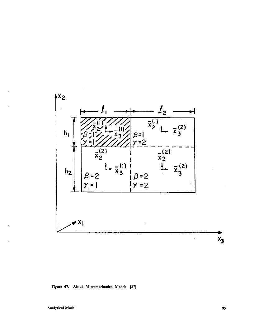
x2

E"-,_.2"L-J,f_ _ . 2 L. (32)hi I'_ _ I'_.//_-_ x 3//I/J = I

...... _;(2) i _(2)"2 ! X2

L -(_} ' L - (2)h , ,8=2 X3 1i,i9=2 X3

Y.= i !Y =2JL !

x}

Figure 47. Aboudi Micromechanical Model: [37]

Analytical Model 95

s q) -- g (s , s C_p) (4.38)

Now dividing through by s gives

1 , (4.39)

The Laplace transform of the composite modulus is now given as a function of s, the Laplace

transform variable. Inverting this expression back into the time domain gives the time domain

viscoelastic solution of the micromechanical model. These expressions for the composite moduli

in the Laplace transform domain are quite complicated and simple methods for inverting the

Laplace transform are difficult to use in this case. A numerical technique developed by Bellman

1411gives a fah-ly simple procedure for inverting the Laplace transform assuming that the time do-

main function is smooth. Since the viscoelastic response of a material is an assumed smooth

function of time, this method works quite weU.

Bellman uses Legendre polynomials to invert a known function of s to its corresponding function

of time. The result of this formulation is a matrix that when multiplied by the values of the Laplace

transform function at given values of s gives the desired result. A more detailed description of this

formulation is given by Bellman 141] and in Appendix A.

4.5 Matrix Modeling

In order to determine the viscoelastic properties of the composite, the viscoelastic properties of the

constituents must be determined. Assuming that the fibers are perfectly elastic, an effective way to

model the matrix is all that is needed. Two models are used here. The first model is the Power-

Law model and it assumes that the viscoelastic response can be modeled as a constant compliance

Analytical Model 96

term plus a power law expression in t. The isotropic creep compliance, S(t), for the Power-Law

model is given by

S(t) = DO+ Ct n (4.40)

where Do is the initial elastic compliance, C and n are measured parameters, and t is time. A

graphical representation of this viscoelastic model is given in Figure 48.

The second model is a Four-Parameter model. This is a mechanical model consisting of springs

and dashpots. The model has a Kelvin element in parallel with a Maxwell element as shown in

Figure 49. The isotropic creep compliance, S(t), for the Four-Parameter model is given by

1 _ e-at) t (4.41)S(t) = -_-- + (1-- q VO

where

2= PlEl (4.42)

Since the epoxy matrix which will be modeled in this study is isotropic, these isotropic creep com-

pliances are all that is needed if it is assumed that the t'oisson's ratio remains constant with time.

From the experimental results, this assumption was shown to be valid and was therefore used in

this study.

In order to use the Correspondence Principle, the Laplace transforms of the creep compliances will

be needed. For the Power-Law model,

Do C F(n + 1)= -7-

Sn+l (4.43)

Analytical Model 97

X

|

J_)O0"0

! ! ! !

TIME

Figure 48. Power Law Graphical Representation

Analytical Model 98

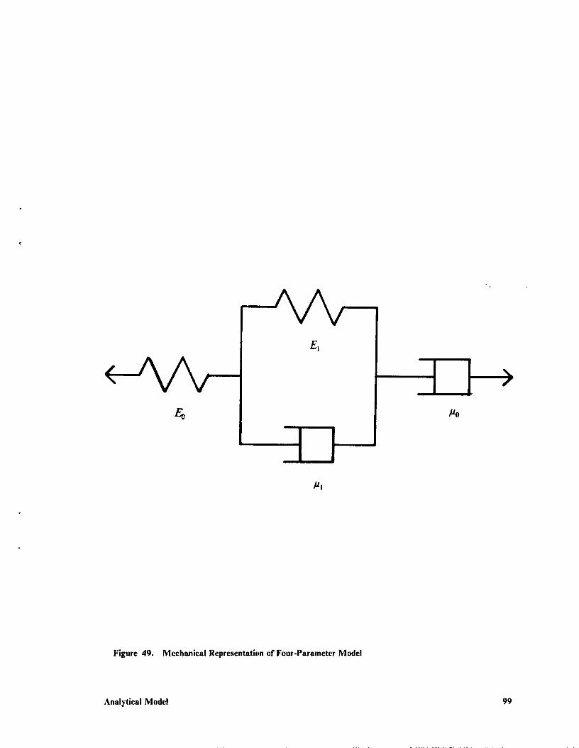
El

I/z0

N.f

]./!

Figure 49. Mechanical Representation of Four-Parameter Model

Analytical Model 99

where F(n + 1) is the Gamma function for (n + 1). Values for the Gamma function can be found

in 1421.

For the Four-Parameter model,

(I/E1) (lIE1) { (1/#°) (4.44)S(s) = (l/E°) + 2s s s+2 s

Since the two micromechanical models are calculated in terms of moduli rather than compliances,

S(s) is converted to C(s) , the Laplace transform of the relaxation modulus, by

C(s) = 1 (4.45)2

s ,_(s)

4.5.1 Parameter Evaluation

In order to use the previously outlined micromechanical models, the parameters to be used in either

the Power-Law model or the Four-Parameter model must be evaluated. The methods used in this

study to determine the needed parameters are outlined below.

For the Power-Law model, the creep compliance is

S(t) = DO+ Ct n (4.46)

Subtracting the elastic compliance from the creep compliance gives the portion of the creep com-

pliance which is time-dependent. This will be called B(t) such that

B(t) = Ct n (4.47)

Taking the base 10 logarittma of both sides gives

Analytical Model 100

log B(t) = log C + n log t (4.48)

In the above expression, log B(t) can be seen as a linear function of log t. The experimental data

normalized with respect to stress level gives the creep compliance. Subtracting the elastic compli-

ance from the creep compliance and plotting the base 10 logarithm of this function versus tile base

10 logarithm of time should approximate a straight line. The slope of tiffs line gives us the exponent

n. Choosing any point on the line and using its coordinates gives the solution for log C wlfich

completes the determination of the two unknown parameters C and n. This process is illustrated

in Figure 50.

For the Four-Parameter model, the evaluation of the unknown parameters is somewhat more ar-

bitrary. Many combinations of the unknown parameters can yield a satisfactory solution."

Choosing a method is therefore more important for the sake of consistency than for accuracy. The

method used in this study is outlined below.

The creep compliance for the Four-Parameter model is

S(t)= 1 1 e-at) t (4.49)- + #o

The spring constant E0 is simply the elastic modulus of the material. This value was evaluated from

the initial elastic response of the matrix. The elastic compliance was subtracted from the compli-

ance at t = 2 hours and multiplied by (1 -l[e). Adding this to the elastic compliance results in a

value hereafter called S l defined as

Sl = (S2h,s- Setasac)(1-1) + Seta_ttc (4.50)

1The value of time at that value of the compliance (S_) was taken as the time constant • = -j-. This

is shown in Figure 51. To solve for El and #0, values of the compliance at t = 30 min and

Analytical Model !01

I1

......... | ......... I ......... I ......... I .........

LOG TIME

Figure 50. Paramctcr Determination for Power-Law Model


t = 2 hours were taken and inserted into equation (4.49). This yields two equations in the two un-

knowns E1 and #0. These equations are easily solved.

4.6 Program Verification

A FORTRAN code known as MICVIS has been written for the MICromcchanical VIScoelastic

fonnulation explained in this chapter. The User's Guide to MICVIS can be found in Appendix

B. To check the validity of the program, readily available data from glass reinforced epoxy was used

with the program [43]. The input parameters were as follows:

• /7.o = 0.563 MSI

• C = .0.188 l/MSI-sec

• n =0.31

• El = 4.37 MSI

• 2 = 0.641 l/sec

• _0 = 392.5 MSI-sec

The glass fiber properties are as follows:

• _ = 12.4 MSI

• v_ = 0.20

• G_ = 5.17 MSI

To verify the program, the transform domain moduli of the matrix were input into the program tbr

not only the matrix, but for the fiber also. In this case, only the isotropic matrix is being modeled.

The creep compliance on output from MICVIS should be the same as the creep compliance of the


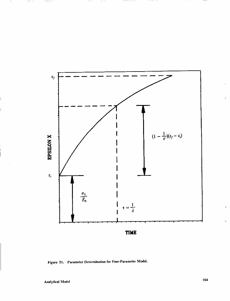
f_

f_

ik

GO

III

II

III

I

Il l

A ..... i

TIME

Figure 51. Parameter Dctermlnation for Four-Parameter Model.


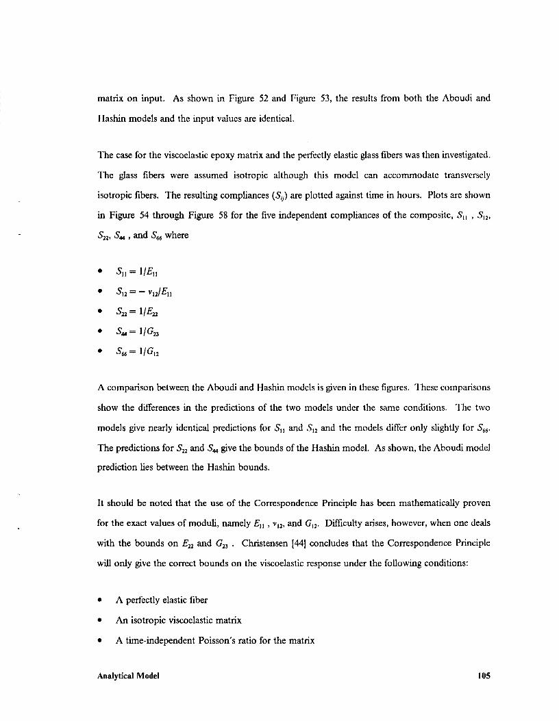
matrix on input. As shown in Figure 52 and Figure 53, the results from both the Aboudi and

| Iashin models and the input values are identical.

The case for the viscoelastic epoxy matrix and the perfectly elastic glass fibers was then investigated.

The glass fibers were assumed isotropic although this model can accommodate transversely

isotropic fibers. The resulting compliances (S0) are plotted against time in hours. Plots are shown

in Figure 54 through Figure 58 for the five independent compliances of the composite, S. , Sl2,

$22, S_, and $66 where

• Sll = l/Etl

• St2 = - _'121E11

• $22 = llFa_

• S_ = llG23

• $66 = 11GI2

A comparison between tile Aboudi and Itashin models is given in these figures. These comp,'u-isons

show the differences in the predictions of the two models under the same conditions. The two

models give nearly identical predictions for Sl_ and St2 and the models differ only slightly for $66.

The predictions for $22and S_ give the bounds of the Hashin model. As shown, the Aboudi model

prediction lies between the Hashin bounds.

It should be noted that the use of the Correspondence Principle has been mathematically proven

for the exact values of moduli, namely EH , vl2, and G12. Difficulty arises, however, when one deals

with the bounds on Fo2 and (723 • Christensen [441 concludes that the Correspondence Principle

will only give the correct bounds on the viscoelastic response under the following conditions:

• A perfectly elastic fiber

• An isotropic viscoelastic matrix

• A time-independent Poisson's ratio for the matrix


MODEL VERIFICATIONABOUDI MODEL

1.80

t.75'

1.70

_1.60

CCJ

!.55

1.50

1.45

1.400

MODEL VERIFICATION

MATRIX RESPONSE

0 MODEL RESPONSE

30 80 90 120

TIME (MIN)

Figure 52. MICVIS Aboudi Model Prediction and Exact Value


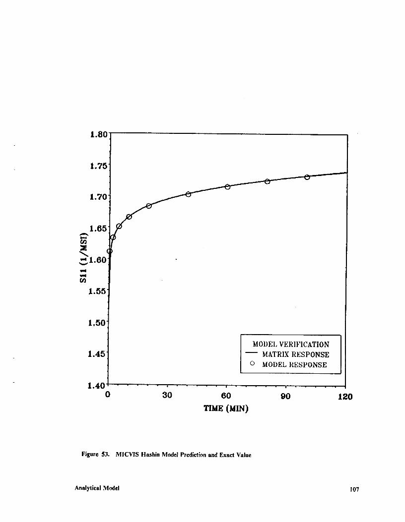
1"80 t

1.751

1"701

_1.60

1.55"

1.50

1.45

!.40 ' '0 30 60

Tree (M_)

MODEL VERIFICATION

-- MATRIX RESPONSE

o MODEL RESPONSE

i

9O

Figure 53. MICV1S ttashin Model Prediction and Exact Value


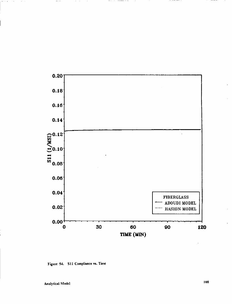
0.20

0.18

0.16

0.14

_0.12tn

0.08

0.06

0.04

0.02

FIBERGLASS

ABOUDI MODEL

HASHIN MODEL

0.000 30 60 90 120

TIME (MIN)

Figure 54. SI 1 Compliance vs. Time


-0.00

-0.01

_,-0.02f_

-0.03

-0.04F1BERGIASS

-- ABOUDI MODEL

--- HASHIN MODEL

-0.05 , , ,0 30 60 90

TIME (MIN)

120

Figure 55. S12 Compliance vs. Time


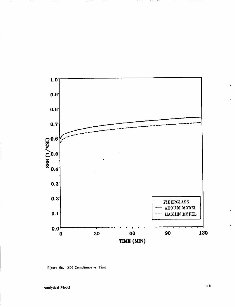
1.0"

0.9

0o8'

0.7

_0.6

_._0cOqO

0.4

0°3'

0.2

0.1

0°0

0 3O

FIBERGLASS

ABOUDI MODEL

HASHIN MODEL

|

6O

TIME (MIN)

|

9O 120

Figure 56. $66 Compliance vs. Time

Analytical Model 1!0

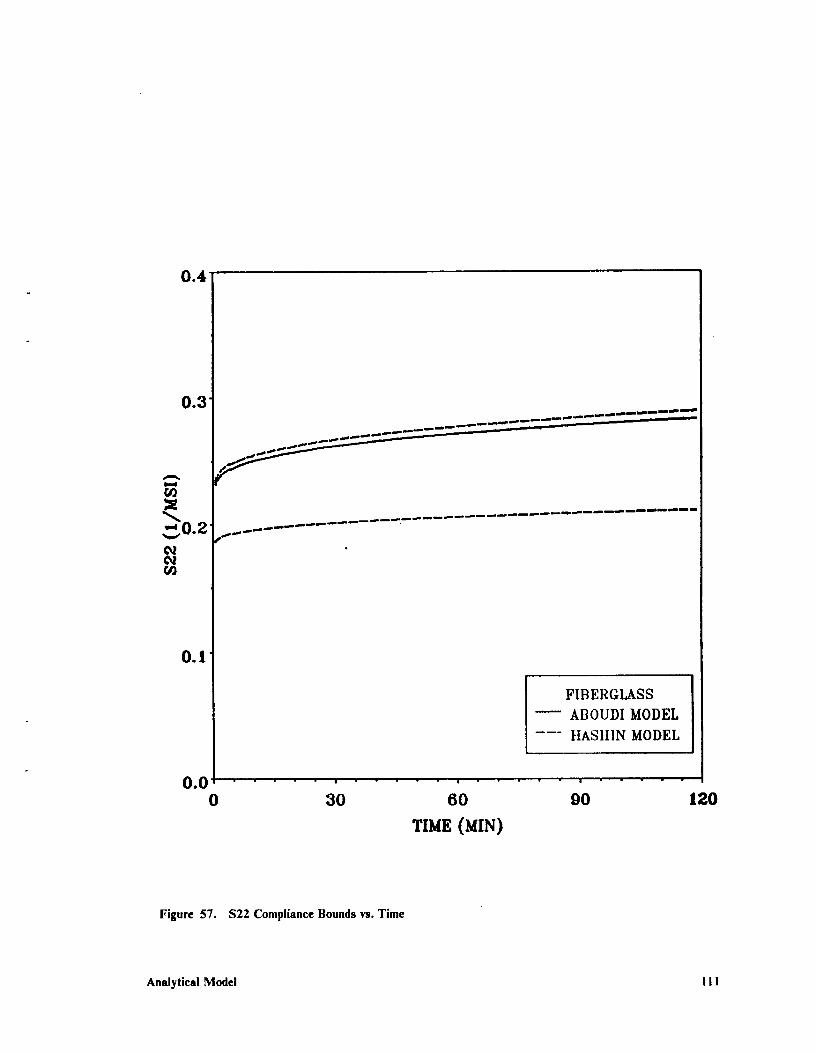
0.4

0.3

A

C,o.2

¢tJ

0.1

, mP m mpm mm N !

m

FIBERGLASS

ABOUDI MODEL

HASHIN MODEL

0 | i m

0 30 60 90

TIME (MIN)

120

Figure 57. $22 Compliance Bounds vs. Time

Analytical Model ! I 1

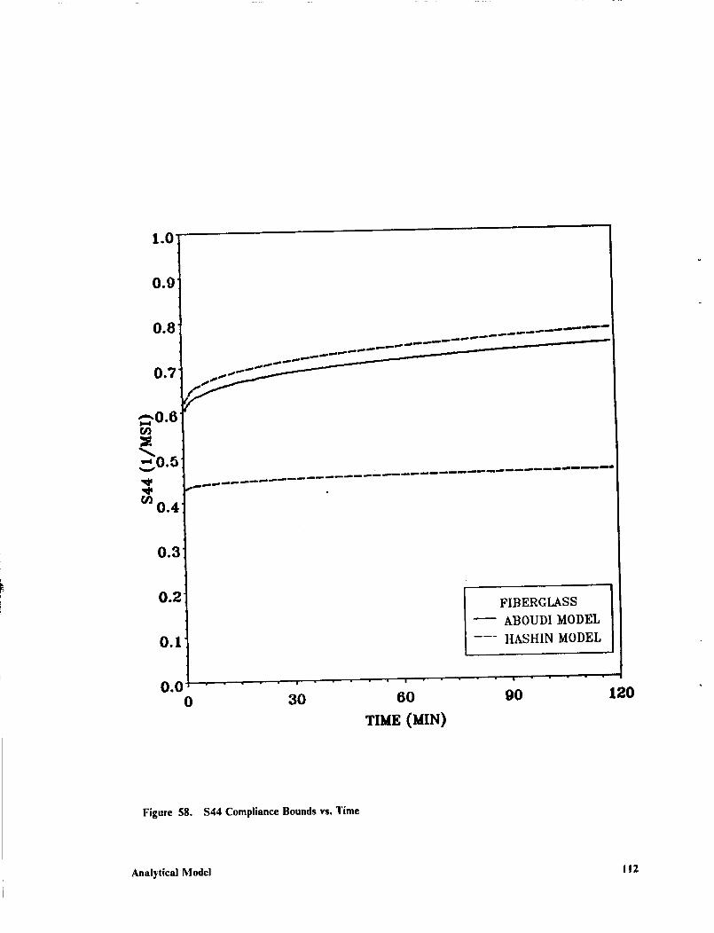
1.0'

0.9

0.8

O.V ¸

O0

0.4

0.3

0.2

O.l

0.00

FIBERGLASS

-- ABOUDI MODEL

--- IIASHIN MODEL

30 60 90 120

'tME(raN)

Figure 58. $44 Compliance Bounds vs. Time


In this example, all of these conditions are met.


5.0 Experimental-Analytical Correlation

Tiffs chapter compares the predictions of the analytical model developed in Chapter 4.0 with the

experimental data presented in Chapter 3.0. Elastic and viscoelastic properties are evaluated lor

both the T300 graphite fibers and the 934 epoxy resin. These properties are then used in MICVIS

to predict the viscoelastic response of the graphite/epoxy composite under the various conditions

tested. These predictions are compared with the experimental data.

5.1 Matrix Modeling

The bulk resin results were modeled using both the Power-Law and Four-Parameter models de-

scribed in Section 4.5. As shown in Section 3.5, the NR, IR, and NE results are very nearly linear.

The IE results for the initial loading were modeled using both the Power-Law and Four-Parameter

model, although linearity cannot be assumed. Plots showing the model approximations to the ex-

perimental data are shown in Figure 59 through Figure 62. Both models do reasonably well in

approximating the experimental data. The Power-Law model seems to do the best job in fitting

the NR, IR, and NE results. The Four-Parameter model seems to do the best job in fitting the IE

Experimental-Analytical Correlation I 14

results.Table8 showstheparametersusedfor thevariousmodels.It shouldbenotedthattile

power-lawexponent,n, evaluatedfortheNR conditionis theidenticalexponentevaluatedby ltiel

andBrinson[45]in theirstudyon thecreepbehaviorof 934resin.

5.2 Model Comparison

In this section, comparison between the model predictions and the experimental data is presented.

The results are given for compliance vs. time where the experimental compliances are computed

by taking the experimental strains and dividing by the stress level. The results from the second

loading were used for the NR, IR, and NE compliance calculations. The results from the initial

loading were used for the IE compliance calculations.

5.2.1 Back Calculation

lsotropic fibers such as glass and boron have measurable properties. Transversely isotropic fibers

such as graphite, on the other hand, have properties that are difficult to experimentally measure.

The fiber elastic properties for graphite fibers, therefore, were determined by back calculation

through the Aboudi micromechanical model. In the case of transversely isotropic fibers, this is an

acceptable method for determination of the fiber elastic properties [34]. Composite properties and

bulk resin properties determined from experiment were used to calculate the fiber elastic properties.

The composite and bulk resin properties for each condition are shown in Table 9. Appendix C

shows tile comparison of these elastic values with results obtained by Milkovich, et al. [16], Reed,

et al. [23], and Fox, et al. [26]. For the composite properties, the axial Young's modulus and axial

Poisson's ratio were taken from the 0 ° tensile test, the transverse Young's modulus was taken from

the 90° test, and the axial shear modulus was taken from the 45 ° off-axis test [46].

Experlmentai-Analytical Correlation I 15

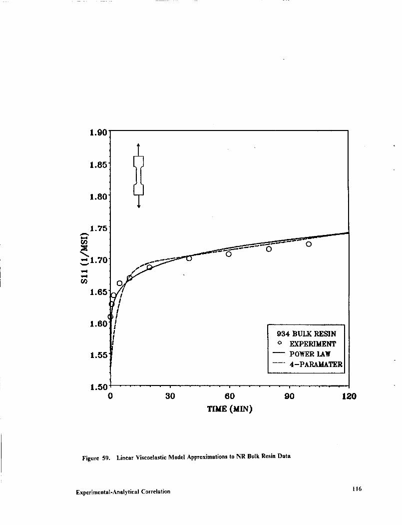
1.90

1.85

1.80

1.75

"-"1.70_, ___

1-65_ I

1.60(:'/I

934 BULK RESIN

o EXPERIMENT

1.55 -- POWER IAW

-- 4-PA_TER

1.500 30 60 90 120

TIME (MIN)

Figure 59. Linear Viscoelastic Model Approximations to NR Bulk Resin Data


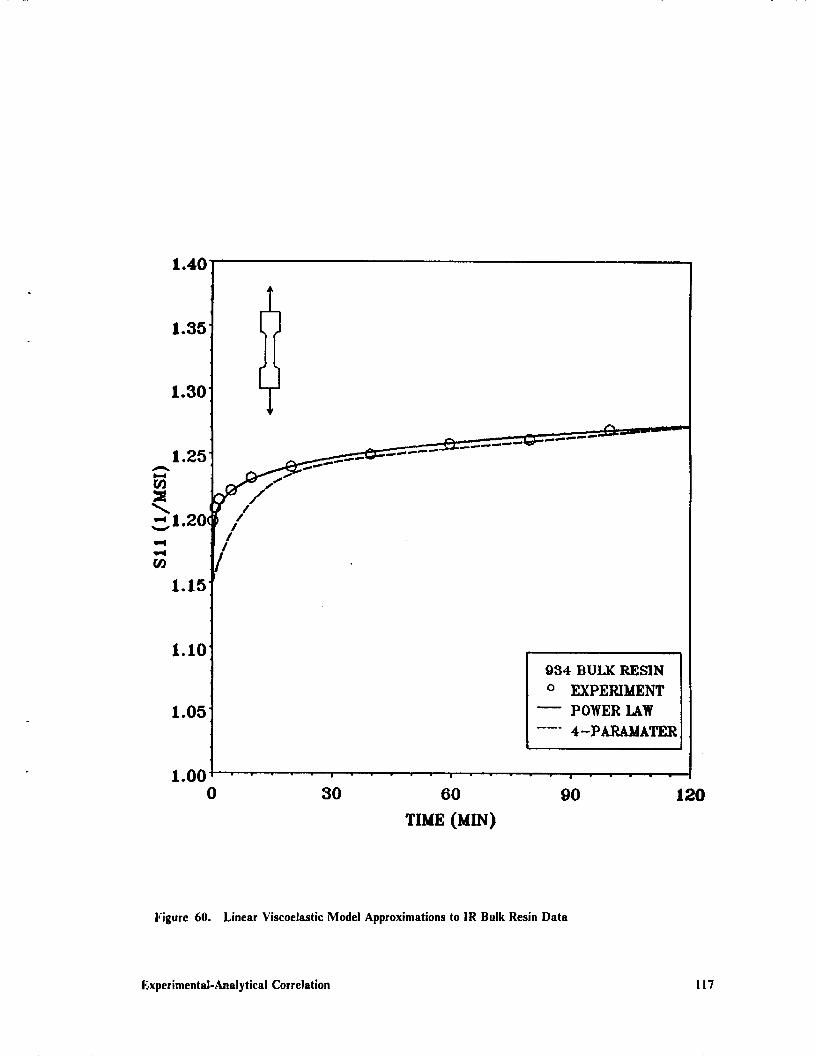
1.40

1.35

1.30

1.15

1.10

1.05

1.00 , ,0 30 60

TIME (MIN)

934 BULK RESIN

o EXPERIMENT

POWER LAW

--- 4-PARAMATER

i

9O 120

Figure 60. Linear Viscoelastic Model Approximations to IR Bulk Resin Data

Experimental-Analytical Correlation !17

2.0

/IIII!!III

934 BULK RESIN

o EXPERIMENT

POWER LAW

-- 4-PARAMATER

0 30 60 90

TIME (MIN)

120

Figure 61. Linear Viscoelastic Model Approximations to NE Bulk Resin Data


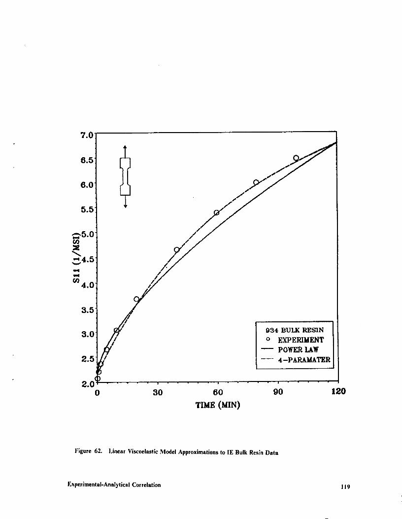
7.0

6.5

6.0

5.5

/

/

934 BULK RESIN

o EXPERIMENT

POWER IAW

4-PARAMATER

2.00 30 60 90

TIME (MIN)

120

Figure 62. Linear Viscoelastic Model Approximations to IE Bulk Resin Data

Experimental-Analytical Correlation 119

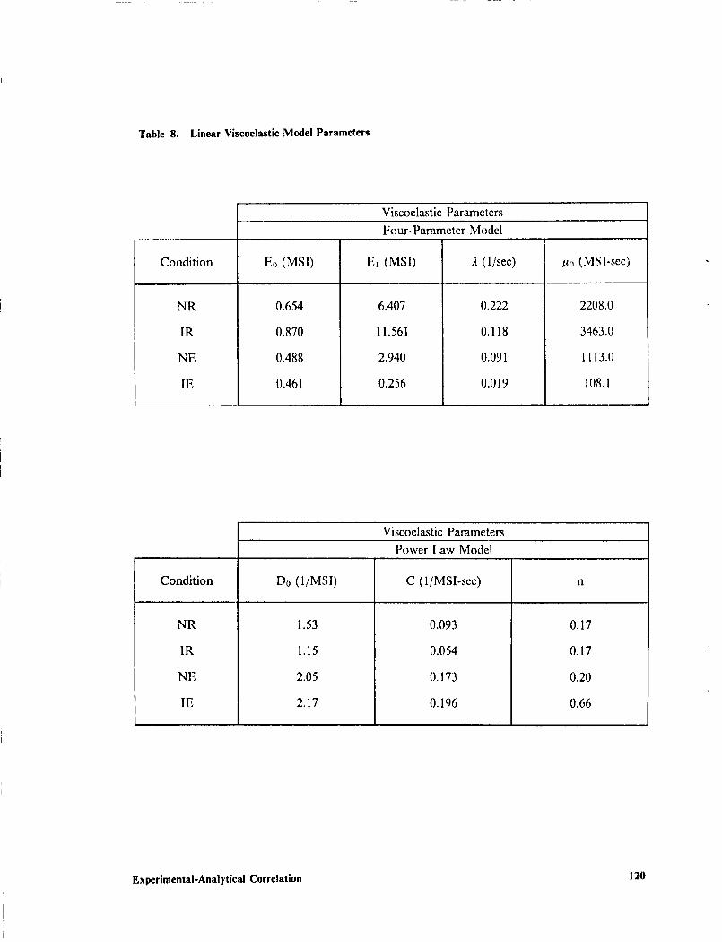
Table8. LinearViscoelasticModelParameters

Viscoelastic Parameters

Four-Parameter Model

Condition E0 (MSI) E1 (MSI) 2 (1/sec) /_o (MSl-sec)

NR

IR

NE

IE

0.654

0.870

0.488

0.461

6.407

11.561

2.940

0.256

0.222

0.118

0.091

0.019

2208.0

3463.0

1113.0

108.1

Viscoelastic Parameters

Power Law Model

Condition Do (1/MSI) C (l/MSI-sec) n

NR

IR

NE

IE

1.53

1.15

2.05

2.17

0.093

0.054

0.173

0.196

0.17

0.17

0.20

0.66

Experimental-Analytical Correlation i 20

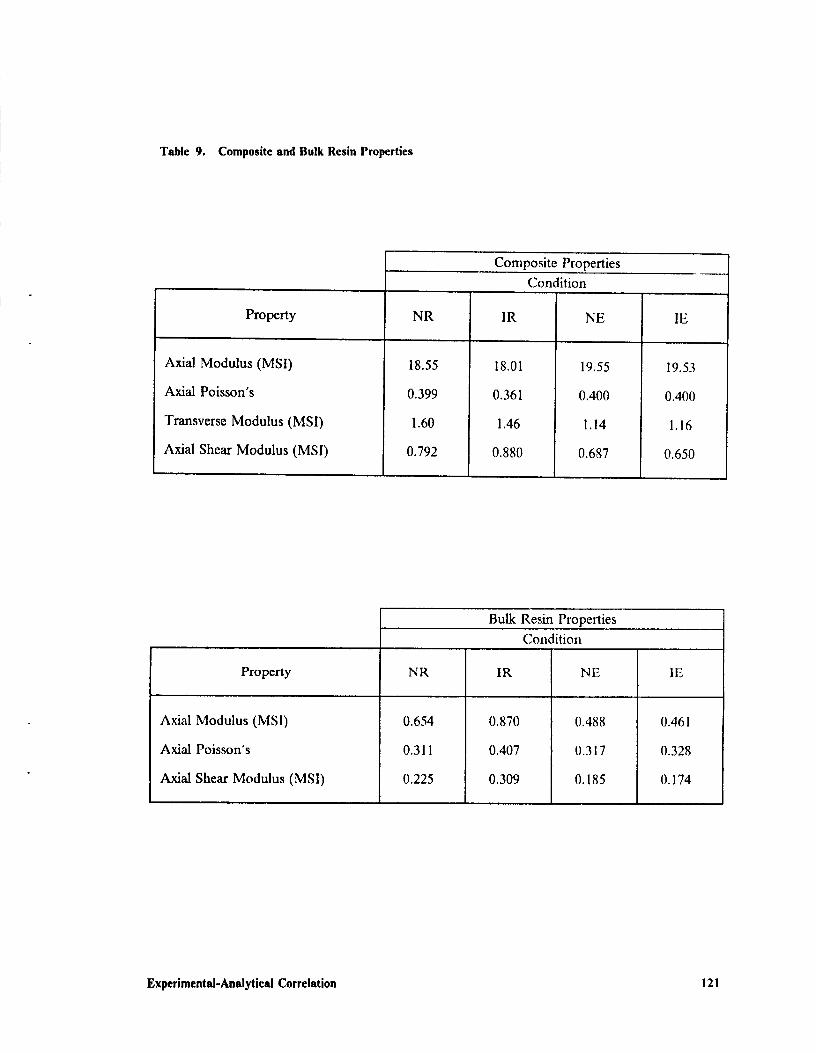
Table9. CompositeandBulkResinProperties

Property

Axial Modulus (MSI)

Axial Poisson's

Transverse Modulus (MSI)

Axial Shear Modulus (MSI)

NR

18.55

0.399

1.60

0.792

Composite Properties

Condition

IR NE

18.01 19.55

0.361 0.400

1.46 1.14

0.880 0.687

IE

19.53

0.400

1.16

0.650

Property

Axial Modulus (MSI)

Axial Poisson's


NR

Bulk Resin Properties

Condition

IR NE

0.654

0.311

0.225

0.870

0.407

0.309

0.488

0.317

0.185

IE

0.461

0.328

0.174


Fiber properties were backed out for each condition and the corresponding fiber elastic properties

are shown in Table I0. It can be seen that the fiber properties vary somewhat under the various

conditions. Reed, et at. [28] did show that radiation does not affect the axial modulus of the

graphite fibers. The significant differences in the backed out fiber properties between the various

conditions are most pronounced for the axial shear modulus and the transverse modulus. These

variations may indicate changes in the axial shear and transverse modulus of the graphite fiber er

may also be an indication of changes in the fiber-matrix interface under conditions of radiation and

temperature.

Fiber properties were also backed out from the Hashin model. These fiber properties are also given

in Table 10. Two properties are given for the transverse modulus to correlate with the upper and

lower bounds for the transverse properties given by the Hashin model. The back calculated fiber

properties from the ttashin model are different from the back calculated fiber properties of the

Aboudi model. It is interesting to note that the back calculated value for the fiber transverse

modulus from the Aboudi model does not fall between the fiber transverse modulus as calculated

from the Hashin model. There also exists large differences in the fiber axial shear modulus obtained

from the two models.

The problem with using the fiber properties from the Hashin model is deciding which bound to

use for the transverse modulus. As shown in Figure 54 through Figure 58, the bounded solutions

from the Hashin model follow fairly similar trends. Choosing a particular bound to use in the

experimental-analytical correlation may indicate a proper trend but give no information on the

proper elastic response. This is obviously a critical parameter to be evaluated. We don't encounter

this problem with the Aboudi model. Due to the difficulties associated with the Hashin bounds,

the model comparison to follow is done only for the Aboudi model.


Table 10. Backed Out Fiber Properties

Backed Out Fiber Properties (Aboudi)

Condition

Property

Axial Modulus (MSI)

Axial Poisson's

NR

29.42

0.443

IR

28.38

0.330

NE

31.09

0.450


Transverse Poisson's


3.67

0.05

6.40

1.75

0.05

2.78

2.15

0.05

9.89

IE

31.07

0.443

2.43

0.05

9.89

Backed Out Fiber Properties (Itashin)

Condition

Property

Axial Modulus (MSI)

Axial Poisson's

Transverse Modulus UB (MSI)

NR

29.42

0.443

2.71

IR

28.38

O.330

0.83

NE

31.09

0.450

1.10

Transverse Modulus LB (MSI)

Transverse Poisson's


1.56

0.05

4.05

0.82

0.05

2.39

0.87

0.05

4.70

IE

31.07

0.443

1.30

0.93

0.05

4.60


5.2.2 Experimental-Analytical Correlation Results

Figure 63 through Figure 67 show the experimental-analytical correlation for tile NR and NE

conditions. Since the NR and IR results are nearly identical for all cases, only the NR

expcrimental-anallytical correlation is detailed in the following figures. The instantaneous elastic

responses of the 90° results and the 45 ° shear results agree exactly since the composite elastic

properties used for back calculation were taken from these tests. For the 10° off-axis shear result,

an error from the experimental results is present. Pindera and I Ierakovich [46] observe that the

measured shear strain in a 10° off-axis test is influenced by constraints resulting from the grips.

The calculated error for the 10° tests with an aspect ratio of 8 used in this study is approximately

40%. This correction was made in the comparison of the 10° shear results. The 10° longitudinal

results shown in Figure 63 compare favorably with the model and the 100 shear results in

Figure 64 show good correlation when the Pindera-Herakovich correction is made. The 45° lon-

gitudinal results in Figure 65 correlate well except for a slight difference in the magnitude of the

elastic response. The 45* shear results in Figure 66 correlate well where no correction factor was

used. The 90° results in Figure 67 "also compare well with the model. The transverse response is

critic_d in the formulation of micromechanical models and it is shown that the Aboudi model pre-

dicts the elastic and viscoelastic response quite well.

5.2.3 IE Results

As discussed in Section 3.6.2, linearity of the IE response cannot be assumed due to the healing

process. The analytical model developed in Chapter 4.0 assumes linearity of the viscoelastic mate-

rial. Disregarding this fact, however, the initial response of the IE bulk resin test was modeled using

the Power-Law and Four-Parameter models. Using the results for the Power-Law model in

MICVIS, the IE composite viscoelastic response is predicted. Sample comparisons with the various

Experimental-Analytical Correlation !24

0.15

0.12"

w.l

•_ 0.06

0.03

10°

__11_13"--13--.... _ ..... -l:----.----.l:. ..... -ta- ......c) o 0 ,0 o Q

0.00 , ,0 30 60

TIME (MIN)

T300/934

o NR EXPERIMENT

NR ABOUDI MODEL

rY NE EXPERIMENT

--" NE ABOUDI MODEL

!

90 120

Figure 63. 10 ° Longitudinal Experimental-Analytical Correlation


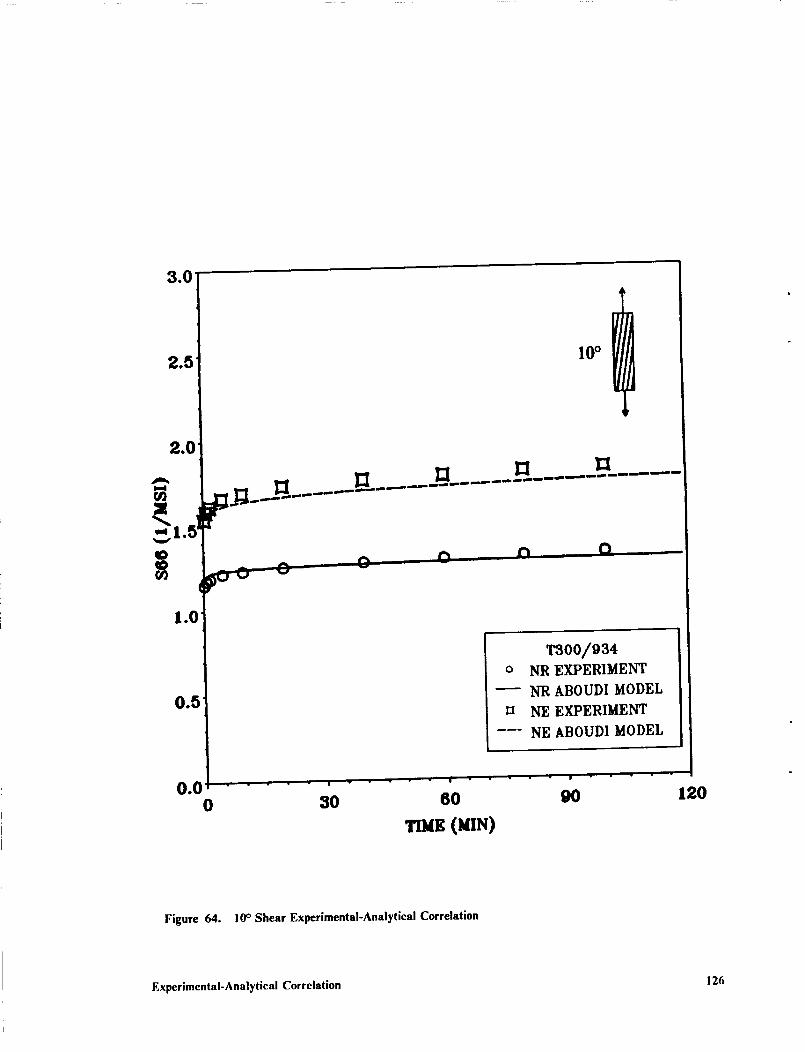
3.0'

2.5

2.0

10°

1.0

0°_ ¸

oO "' .... |

0 30

T300/934

o NR EXPERIMENT

NR ABOUDI MODEL

n NE EXPERIMENT

--- NE ABOUDI MODEL

. i _ • t . . • $ , . . .

80 90 120

TIME (MIN)

Figure 64. I0° Shear Experimental-Analytical Correlation


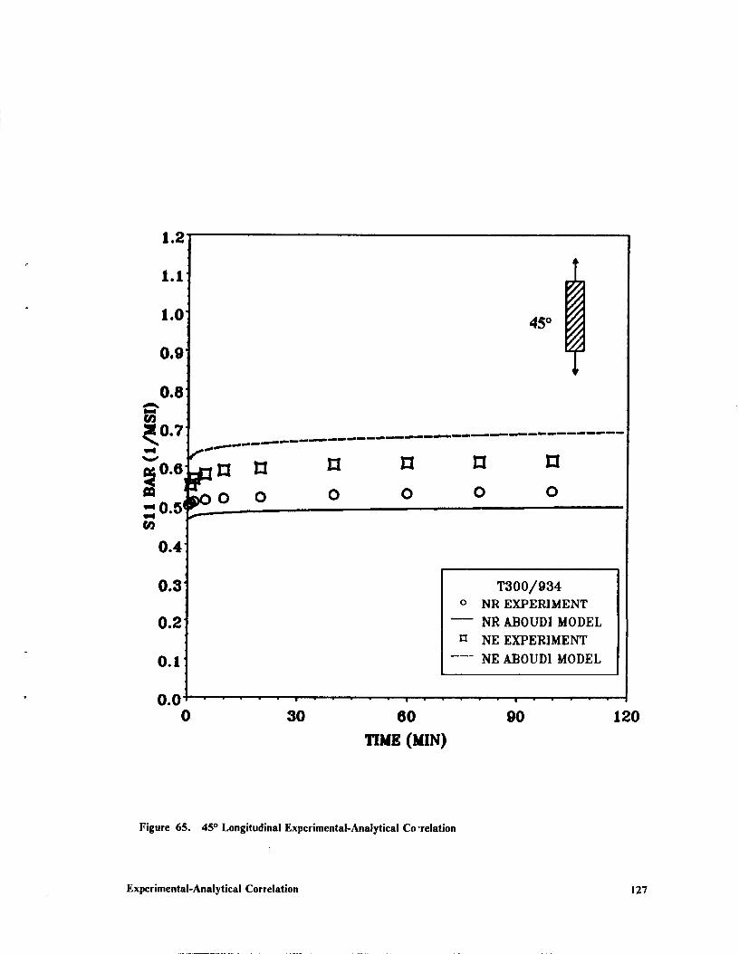
1.2

1.1

1.0

0.9

V

0.5_ _ O Ow=l

0.4

0.3

0.2

0.1

0.00

45 °

m m m I m m mmm m ml

_ _,_,wmm_m_,_'_ _m' mm_m,_ mmwm_ amw m _'_m _im, am_mmU_mmm_mm *m atom _m

I:I I:I Izl I:I

0 0 0 0i |

T300/934

o NR EXPERIMENT

m NR ABOUDI MODEL

t_ NE EXPERIMENT

--- NE ABOUDI MODEL

I | |

30 60 90 120

TIME (MIN)

Figure 65. 45 ° Longitudinal Experimental-Analytical Co "relation


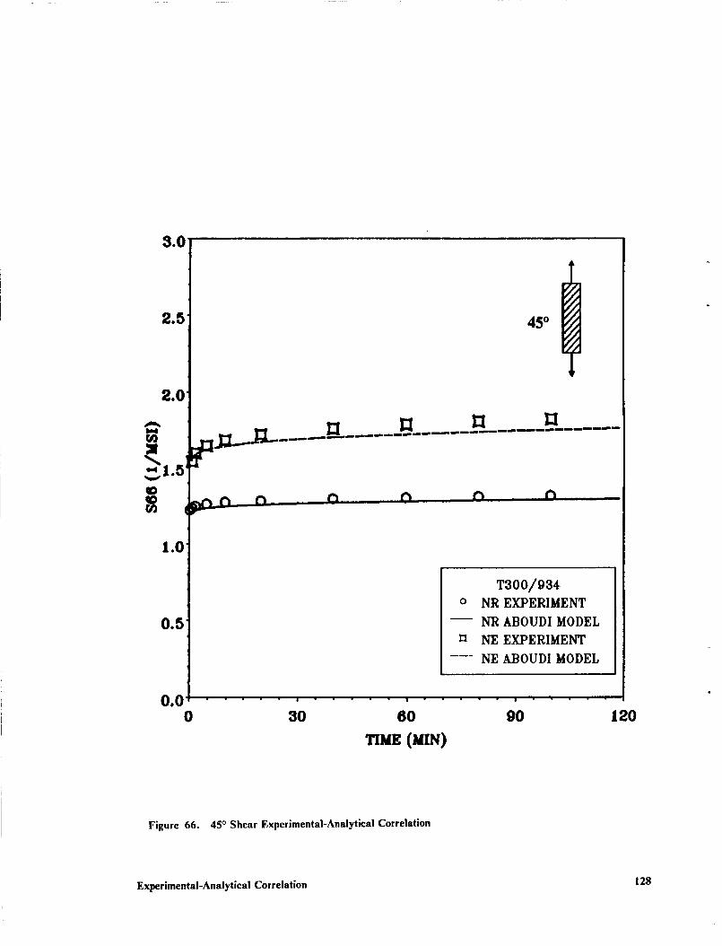
3.0

2.5'

2°0'

45 °

0.5

O0 ' '

0 30 60

TIME (MIN)

T300/934

o NR EXPERIMENT

ABOUDI MODEL

_ EXPERIMENT

--- NE ABOUD] MODEL

I

90 120

Figure 66. 45 ° Shear Experimental-Analytical Correlation


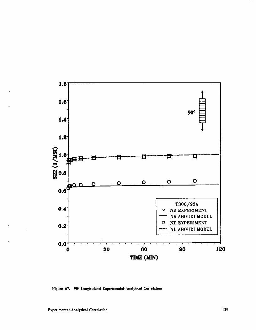
1.8

1.6

1,4'

1.2

A

90 °

_ |

e_0.8 | o0.6 J'_C_-o O 0 0 0

0o4

0.2

*O w |

0 30 60

TIME (raN)

O

T300/934

NR EXPERIMENT

NR ABOUDI MODEL

NE EXPERIMENT

NE ABOUDI MODEL

|

9O

o,

120

Figure 67. 90 ° Longitudinal Experimental-Analytical Correlation


tests are shown in Figure 68 through Figure 70. The 10° longitudinal results in Figure 68 show

a reasonable correlation between experiment and the analytical model although it is not as good a

correlation as seen for the NR and NE results. The 45° shear results in Figure 69 show a less ac-

curate correlation between theory and experiment. The 90 ° longitudinal results in Figure 70 show

a very poor correlation. In this case, the model significantly over-predicts the experimental result.

The poor correlation may be due to the healing process which introduces complications in the as-

sumption of linear viscoelasticity. The poor correlation may also be an indication that the rate of

healing in the bulk resin is different than the rate of healing in the composite.


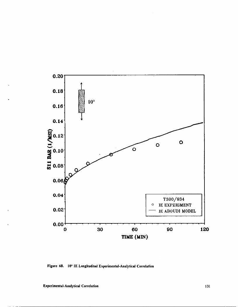
0.20

0.18

0.16

0.14

_'0.12

0.10

Iml

0.08

0.06

0.04

0.02

lO °

0.00 ' '0 30 60

TIME (MIN)

o

T300/934

IE EXPERIMENT

IE ABOUDI MODEL

|

9O 120

Figure 68. 10° IE Longitudinal Experimental-Analytical Correlation


45 °

0

0

0

0 0

1.0

o

T300/934

IE EXPERIMENT

IE ABOUDI MODEL

0.00 30 6O

TIME (MIN)

9O 120

Figure 69. 45° IE Shear Experimental-Analytical Correlation


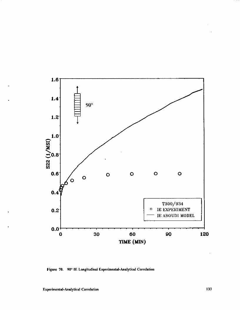
1.6

1.4

1.2

1.0A

o.8

0.6

0.41

0.2

0.00

O0 0 0 0

I i

30 60

"rIME (MIN)

0

T300/934

]E EXPERIMENT

IE ABOUD1 MODEL

|

90 120

Figure 70. 90 ° IE Longitudinal Experimental-Analytical Correlation


6.0 Conclusions and Recommendations

The results of this study indicate that electron radiation has a significant effect on the time-

dependent response of T300/934 graphite/epoxy at + 250 °F, a temperature very near the glass

transition temperature of the irradiated composite. Radiation-induced chain scission of the epoxy

network allows for increased chain mobility near the glass transition temperature. Chain mobility

increases the viscoelastic behavior of the composite and also pemaits free radicals and ionic centers

broken off from molecular chains during irradiation to recombine and form cross-links. Over time,

this recombination or healing restricts further chain mobility and therefore decreases subsequent

viscoelastic behavior of the composite.

The following list summarizes the significant conclusions of this study.

• Radiation has little effect on the creep response of T300/934 graphite/epoxy at 72 °F.

• Radiation has a significant effect on the creep response of T300/934 graphite/epoxy at + 250

°F.

• Itealing of radiation induced chain scission in the 934 resin structure is observed at + 250 °F.

Conclusions and Recommendations 134

Only the the time-dependent behavior of the irradiated composite at + 250 °F is affected by

healing. The elastic response is linear with time. It is hypothesized that radiation and healing

affect only secondary bonds in the epoxy molecular network and that these conditions have

no effect on the primary bonds of the molecular structure.

• Trends in the creep response of the bulk 934 resin are similar to the creep response of T300/934

graphite/epoxy under various conditions of temperature and radiation exposure.

• Creep is most pronounced in off-axis orientations of unidirectional T300/934 graphite/epoxy

where a 1-2 shear stress is present.

The micromechanical approach to viscoelasticity formulated in this study gives accurate prcd-

ictions of the viscoelastic response for unidirectional fiber reinforced composites. The model

correlates best with linearly viscoelastic behavior with relatively small creep strains. The model

breaks down for the IE response when healing is present.

The following list outlines recommendations for further work in tiffs area.

Further evaluate the healing process in the irradiated 934 epoxy resin. Stress, temperature, and

time dependence of healing effects need to be quantified by conducting additional tests under

various conditions of the above parameters.

• Model the healing process to better predict the time-dependent response of the IE condition.

• Modify MICVIS to incrementally predict nonlinear viscoelastic behavior of fiber rehdorced

composite materials.

• Implement the Correspondence Principle with the Bellman Method to predict viscoelastic be-

havior of additional composite configurations such as laminates and tubes.

Conclusions and Recommendations 135

7.0 References

l°

.

.

o

.

°

,

°

.

10.

Termey, D.R., Sykes, G.F., and Bowles, D.E., "Composite Materials for Space Struc-tures", Proceedings of the Third European Symposium on Spacecraft Materials in SpaceEnvironments, October 1985, pp. 9-21.

Termey, D.R., "Spacecraft Materials Research - A NASA Perspective", Large Space An-tenna Systems Technology - 1982, Part I, NASA CP-2269, pp. 213-239.

Lubin, G. and Dastin, S.J., "Aerospace Applications of Composites", ltandbook ofComposites G. Lubin, Ed., Von Nostland Reinhold Company, Inc., New York, pp.722-743.

Hillesland, H.L., "Advance Composites Hardware Utilized on the Intelsat V Spacecraft",SAMPE Symposium�Exhibition, Vol. 24, pp. 202-211.

Archer, J.S. "High Performance Parabolic Antenna Reflectors _, Proceedings AIAA 7thCommunications Satellite Systems Conference, San Diego, CA, 24-27 April 1978, AIAAPaper No. 78-593, pp. 442-447.

Grounder, R.N., "Advanced Composite Antenna Reflectors for Communication Satel-lites", SAMPE Journal 19(3), pp. 11-14.

Quails, J.P., "Graphite Epoxy Satellite Structure Development Program", NationalSAMPE Technical Conference, Vol. 14, pp. 513-520.

Ginty, C°A. and Chamis, C.C., "Select Fiber Composites for Space Applications : AMechanistic Assessment", SAMPE 29th National Symposium, 3-5 April 1984, pp.979-993.

Leung, C.L., "Space Environmental Effects on Graphite/Epoxy Composites", CompositesFor Extreme Environments, ASTM STP 768, N.R. Adsit, Ed., American Society forTesting and Materials, 1982, pp. 110-117.

Sykes, G.F., Slemp, W.S., "Space Radiation Effects on an Elastomer-ToughenedEpoxy-Graphite Composite", 30th National Symposium/Exhibition Society for the Ad-vancement of Materials and Process Engineering, 19-21 March, 1985, Anaheim, CA.

References 136

11.

12.

13.

14.

15.

16.

17.

18.

19.

20.

21.

22.

23.

24.

25.

26.

Sykes, G.F., Funk, J.G., and Slemp, W.S., "Assessment of Space Enviromnent InducedMicrodarnage in Toughened Composite Materials", 18th International Technical ('o11-ference, Society for the Advancement of Materials and Process Engineering, 7-9 October,1986, Seattle, WA.

Alfrey, T. Jr., Mechanical Behavior oftligh Polymers, Interscience Publishers, New York,1948.

Tumer, A. and Gumee, E.F., Organic Polymers, Prentice-HaU Series in Materials Science,Englewood Cliffs, NJ, 1967.

Doolittle, A.K. and Doolittle, D.B., Journal of Applied Physics, Vol. 28, p. 373, 1957.

Ferry, J.D., Viscoelastic Properties of Polymers, John Wiley and Sons, New York, 1970.

Milkovich, S.M., Herakovich, C.T., and Sykes, G.F., "Space Radiation Effects on theThermo-Mechanical Behavior of Graphite-Epoxy Composites", Journal of CompositeMaterials, Vol. 20, November 1986.

Bowles, D.E., Tompkins, S.S., and Sykes, G.F., "Electron Radiation Effects on theThermal Expansion of Graphite/Resin Composites", AIAA 19th Thermophysics Con-ference, 25-28 June 1984, AIAA-84-17(14.

I laskins, J.F., "Advanced Composite Design Data for Spacecraft Structural Applications",SAMPE 12th National Technical Contbrence, 7-9 October, 1980.

Tompkins, S.S., Sykes, G.F., and Bowles, D.E., "The Thermal and Mechanical Stabilityof Composite Materials for Space Structures", IEEE/ASM/ASME/SME Space TechConference, 23-25 September 1985, Anaheim, CA.

Chapiro, A., "Radiation Induced Polymerizations in the Vicinity of Glass TransitionTemperatures", Proceedings of the Twenty-Second Nobel Symposium, 20-22 June 1972,Sodergam, Lidingo, Sweden.

Tenney, D.R., Sykes, G.F., and Bowles, D.F., "Space Environmental Effects on Materi-als", AGARD Environmental Effects on Materials for Space Applications, Toronto,Canada, 22-24 September 1982.

Garrett, tt.B., "Review of the Near-Earth Spacecraft Environment", SPIE, Vol. 216,Optics in Adverse Environments, 1980, pp. 109-115.

Reed, S.M., Iterakovich, C.T., and Sykes, G.F., "Influence of Electron Radiation andTemperature on the Cyclic, Matrix Dominated Response of Graphite-Epoxy", Journalof Composite Materials, Vol. 21, July 1987.

Hagiwara, M., and Kagiya, T., "[tigh Energy Degradation and Stabilization of Polymers",Degradation and Stabilization of Polymers, Jellinek, H.II.G., Ed., Elsevier, New York,1983.

Fox, T.G., "Polymer Flow in Concentrated Solutions and Melts", Structure and Proper-ties of Polymers, Tobolsky, A.F., Ed., John Wiley Interscience Publishers, New York,1965.

Fox, D.J., Ilerakovich, C.T., and Sykes, G.F., "Degradation of Graphite-Epoxy Due toElectron Radiation", ASME Journal of Engineering Materials Technology, (ha press 1988).

References 137

27.

28.

29.

30.

31.

32.

33.

34.

35.

36.

37.

38.

39.

40.

41.

42.

43.

Milkovich,S.M., Sykes,G.F., and Herakovich,C.T., "Space Radiation Effects onGraphite/Epoxy Composite Materials", Interim Report 45, The NASA-Virginia TechComposites Program, VPI-E-84-20, June 1984.

Reed, S.M., Herakovich, C.T., and Sykes, G.F., "I'he Effects of Space Radiation on aChemically Modified Graphite/Epoxy Composite Material", Interim Report 60, TheNASA-Virginia Tech Composites Program, VPI-E-86-19, October 1986.

Fox, D.J., Sykes, G.F., and Ilcrakovich, C.T., "Space Environmental Effects onGraphite/Epoxy Compressive Properties and Epoxy Tensile Properties", Interim Report63, The NASA-Virginia Tech Composites Program, VPI-E-87-13, July 1987.

D638-82a, "Standard Test Method for Tensile Properties of Plastics", 1984 Annual Bookof ASTM Standards, Section 8, Vol. 08.01, American Society for Testing and Materials,1984, Philadelphia.

Micro-Measurements, M-Line Accessories, Instruction Bulletin B-137-11.

Signor, L.L., 'q'he Effect of Temperature on the Creep Response of 934 Epoxy Resin",Senior Project Final Report, VPI, June 1987.

Hidde, J.S., Beuth, J.L. Jr., and tterakovich, C.T., "MATPACO v2.0: A PC-BasedSoftware Package for Materials Testing", January 1988.

Tsai, S.W., Composites Design, Third Edition, Think Composites Publishers, Dayton,Ohio, 1987.

Chi'istensen, R.M., Theory of Viscoelasticity." An Introduction, Second Edition, AcademicPress, New York, 1982.

Hashin, Z., 'q'heory of Fiber-Reinforced Materials", NASA Contractor Report 1974,March 1972.

Aboudi, J., "A Continuum Theory For Fiber-Reinforced Elastic-Viscoplastic Compos-ites", International Journal of Engineering Science, Vol. 20, No. 5, pp. 605-621, 1982.

Aboudi, J., "Closed Form Constitutive Equations for Metal Matrix Composites", Inter-national Journal of Engineering Science, Vol. 25, No. 9, pp. 1229-1240, 1987.

Pindera, M-J, and Aboudi, J., "Micromechanical Analysis of Yielding of Metal MatrixComposites", International Journal of Plasticity (1988 in press).

Pindera, M-J, Aboudi, J., and Herakovich, C.T., "Nonlinear Response ofBoron/Aluminum Under Combined Loading", IUTAM/ICM Symposium on Yielding,Damage, and Failure of Anisotropic Solids, Grenoble, France, August 1987.

BeUman, R., Kalaba, R.E., and Lockett, J.A., Numerical Inversion of the Laplace 7"rans-form, American Elsevier I'ublislfing Company, Inc., New York, 1966.

tlilldebrand, F.B., Advaneed Calculus for Applications, Second Edition, Prentice-I laU,Inc., Englewood Cliffs, N J, 1976.

Pindera, M-J, Lazarus, B.E., "Program User's Guide for VISCO: Evaluation of EffectiveViscoelastic Properties", MSC TIR 1311, Materials Science Corporation, November1982.

References 138

4, Christensen, R.M., Mechanics of Composite Materials, Jolm Wiley and Sons, New York,1979.

45. Hiel, C., Brinson, H.G., "q'he Nonlinear Viscoelastic Response of Resin Matrix Com-posite Laminates," VPI-E-83-6, Virginia Polytechnic Institute and State Univcrsity, June1984.

46. Pindera, M-J and Ilerakovich, C.T. "Shear Character_ation of Unidirectional Compos-ites with the Off-Axis Tension Test", Experimental Mechanics, Vol. 26, No. 1, pp.103-112, March 1986.

References 139

Appendix A. Bellman Method

As discussed in Section 4.2, use of the Correspondence Principle can lead to a wide range of

viscoelastic solutions from the corresponding elastic solutions. The difficulty arises in inverting the

given expression in the Laplace Transform domain to the time domain. Except for very simple

problems, the function

"_u(s)= s CUkl(s)_kl(s) (A.l)

will be a very complicated function of s. Inverting this is difficult and thus an approximate means

of inverting these expressions to the time domain is typically employed. A method proposed by

Bellman [41] has been chosen in this investigation. It is briefly outlined below.

A function u(t) is desired such that

F(s) = e-Stu(t)dt (A.2)

where F(s) is a known function of the Laplace transform variable s.

expressed as a fmite sum of the form

First, the integral in (A.2) is

Appendix A. Bellman Method 140

N

i= I

(,.I.3)

where flxi) are values of the function f(x) at the points x_ and w_ are the corresponding weight fac-

tors.

The next step is to express the function f(x) as a finite sum such that

N

jCx)= ,bkPk(x)k=O

(A.4)

where Pk(x) are some known functions of x. The choice of P,(x) is the key here. Choosing P,(x)

to be the Legendre polynomials of order k which are orthogonal polynomials helps to solve the

problem. On the interval [ -1,1] this orthogonality condition states that

ff_ P,nPndx = O m _ n (A.5)1

P2.(x)dx = (A.6)2

! (2n + 1)

Multiplying the function f(x) by P_(x) and integrating from [ -I, 1] gives

1 N

; x=r[Z ,+xJ- 1Lk=0 J

(A.7)

By the orthogonality condition of (A.5) and (A.6) this reduces to


x)e_x)dx = btf e](x)dx (A.8)

This gives

bt = l________)1(2/+ r" flX)Pl(x)dx (A.9)2 j_l

Assuming now that the integration in (A.3) is evaluated on the interval [ -1,1] gives w_ and x,. It

is required that (A.3) be exact for any polynomial of degree less than or equal to 2N - 1 by a pro-

cedure proposed by Gauss.

Lettingflx) = x*P,v(x) in (A.2) gives

N

_'_ XkPN(x)dx = EwixkpN(xi)

1 i=1

(A.IO)

For k < N,

(A.II)

This results in

N

i=l

(A.12)

For (A.12) to hold true, assuming that the x_ are distinct and the w,. are non-zero, the x_ must be

the zeroes of P_x). Tim zeroes of a Legendre polynomial are distinct.


To determine the weight factors, w_, let the function f(x) in (A.3) be

l(x)=P_x)

(x - x_)p'N(x¢)(A,13)

It can be seen that

J(xy) = 0 y 4: i (d. 14)

J_xt)= l j=_

Substituting this into (A.3) gives

f l PN(x) (A. 15)w_= (x - x_)p'_x_)-1

Using (A.15) gives a solution for u(t) in (A.2). First, a change of variables is performed in (A.2)

where x = e -t . This results in

F(s) = f01 x s-I u( -logx)dx (A. 16)

Since the evaluation of the weights and zeroes of the Legendre polynomials are on the interval

[ -1,1], a shifting to the interval [0,1] is desired. This shifting is accomplished by simply letting

e_x) = t,_ l - 2x) ¢A.17)

where P'u(x) are the shifted Legendre polynomials. This gives

x_ = 2(x_- l) (,4.18)

w_ = 2w_ (A. 19)


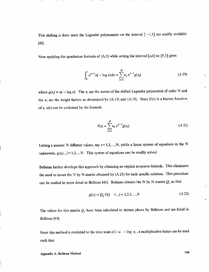
Thisshiftingis donesincetheLegendrepolynomialson theinterval[-1,1] arereadilyavailable

1421.

Now applying the quadrature formula of (A.3) while setting the interval [a,b] to [0,1] gives

N

log =Xw,i=1

(A.2o)

where g(xi) = u( - log x). The x, are the zeroes of the shifted Legendre polynomial of order N and

the wi are the weight factors as determined by (A.15) and (A.19). Since F(s) is a known function

of s, u(t) can be evaluated by the formula

N

F(s) = Zwi xS-l g(x_)i= 1

(A.21)

Letting s assume N different values, say s= 1,2...... N, yields a linear system of equations in the N

unknowns, g(xi), i = 1,2 ..... N. This system of equations can be readily solved.

Bellman further develops this approach by obtaining an expLicit inversion formula. This eliminates

the need to invert the N by N matrix obtained by (A.21) for each specific solution. This procedure

can be studied in more detail in Bellman [41]. Bellman obtains the N by N matrix Q_jso that

g(x i) = Q_ F(I) i, j = 1,2,3 ...... N (A.22)

The values for this matrix Q,s have been calculated to sixteen places by Bellman and are listed in

BeUman 1411.

Since this method is restricted to the time scale of t = - log x_, a multiplicative factor can be used

such that


N

F(s/a) Ea = wixS-lu(--al°gxi)

i=1

(A.23)

This allows one to obtain the values of u(t) at any given time t and still use the same inversion

matrix Q,j, thus eliminating the need to repeat the entire procedure from the beginning.


Appendix B. MICVIS User's Guide

B.1 Introduction

MICVIS is a FORTRAN program written to evaluate the effective viscoelastic properties of a

unidirectional composite material. These properties are calculated using the properties of the con-

stituent materials as input assuming a perfectly elastic, transversely isotropic fiber and an isotropic,

viscoelastic matrix with a time-independent Poisson's ratio. The program can be easily modified

to take into account a viscoelastic fiber and/or a varying Poisson's ratio. These properties, however,

were not needed for the problem this program was intended to solve and the reader can modify this

program if so desired to meet these conditions.

The user needs to have the following information for input:

Fiber

• E T

• v A

= Axial Young's Modulus

= Transverse Young's Modulus

= Axial Poisson's Ratio

Appendix B. MICVIS User's Guide 146

= Transverse Poisson's Ratio

= Axial Shear Modulus

Matrix

• E.

V A

C,n

El, ,_, #o

= Axial Young's Modulus

= Axial Poisson's Ratio

= Parameters for Power-Law Model

-- Parameters for Four-Parameter Model

Other Input

• vI

• F

= Fiber Volume Fraction

= Gamma Function evaluation tbr exponent n

The output of the program gives the effective creep compliances of tile composite:

Output

• Sll(t) = Axial Creep Compfiance

• Sl2(t ) = Axial Poisson Creep Compfiance

• Szz(t) = Transverse Creep Compliance

• S_(t) = Transverse Shear Creep Compliance

• $66(t) = Axial Shear Creep Compliance

This program is based on the elastic-viscoelastic Correspondence Principle. Two elastic microme-

chanical models developed by Aboudi [37] and ttastfin 136] respectively are converted to the

viscoelastic time domain by use of the Correspondence Principle [35]. A Laplace Transform in-

version scheme developed by Bellman is used to make this conversion. Two different models are

employed to characterize the viscoelastic behavior of the matrix, namely the Power-Law Model and

the Four-Parameter Model. These procedures can be found in Chapter 4.0.


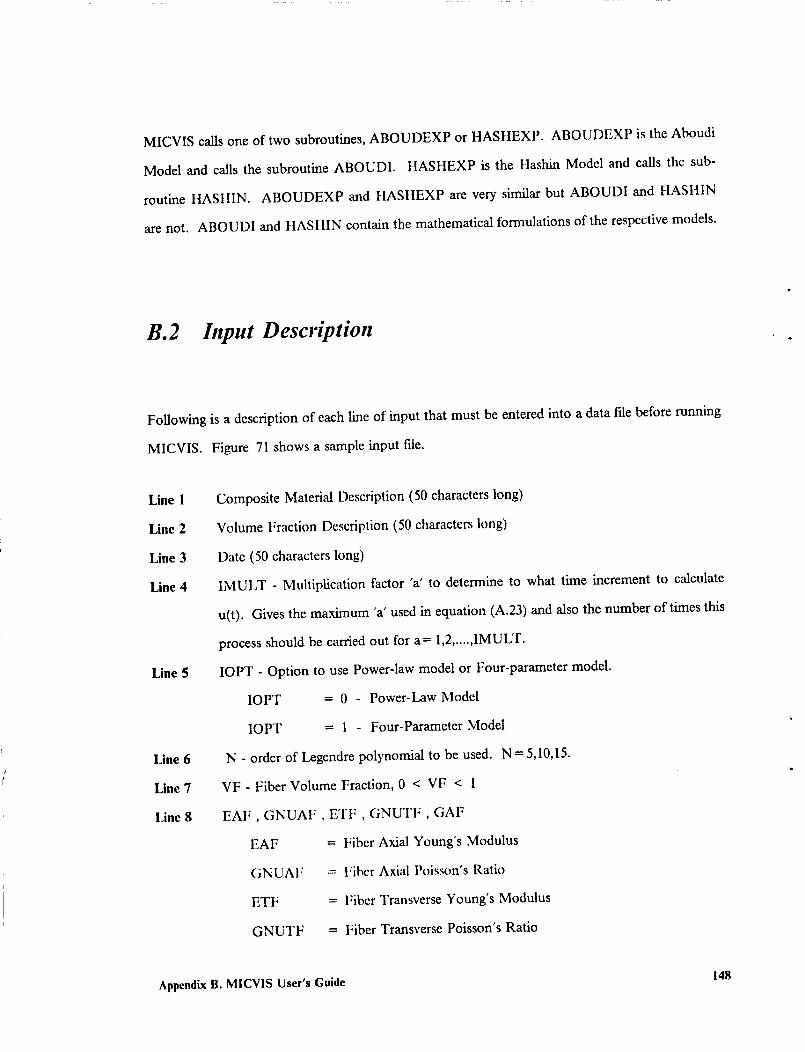
MICVIScallsoneof twosubroutines,ABOUDEXPor HASHEXP.ABOUDEXP is the Aboudi

Model and calls the subroutine ABOUDI. tIASHEXP is the ttashin Model and calls the sub-

routine HASIIIN. ABOUDEXP and HASHEXP are very similar but ABOUDI and HASHIN

are not. ABOUDI and HASttlN contain the mathematical formulations of the respective models.

B.2 Input Description

Following is a description of each line of input that must be entered into a data fde before running

MICVIS. Figure 71 shows a sample input ftle.

Line I

IJne2

Line3

Line4

Line 5

Line 6

Line 7

Line 8

Composite Material Description (50 characters long)

Volume Fraction Description (50 characters long)

Date (50 characters long)

IMULT - Multiplication factor "a' to determine to what time increment to calculate

u(t). Gives the maximum "a' used in equation (A.23) and also the number of times this

process should be carried out for a= 1,2...... IMULT.

IOPT - Option to use Power-law model or Four-parameter model.

IOPT = 0 - Power-Law Model

IOPT = 1 - Four-Parameter Model

N - order of Legendre polynomial to be used. N = 5,10,15.

VF - Fiber Volume Fraction, 0 < VF < 1

EAF , GNUAF , ETF , GNUTF , GAF

EAF

GNUAF

ETF

GNUTF

= Fiber Axial Young's Modulus

= Fiber Axial Poisson's Ratio

= Fiber Transverse Young's Modulus

= Fiber Transverse Poisson's Ratio

Appendix B. MICV1S User's Guide 148

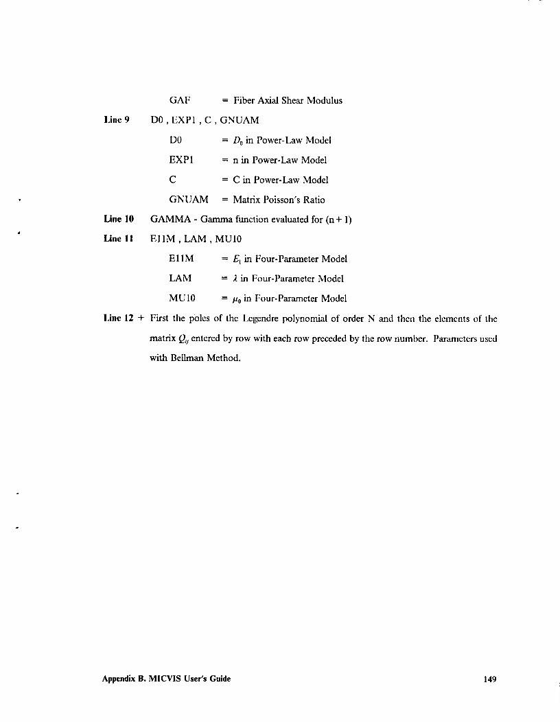
l,ine9

LineI0

LineI1

GAF = Fiber Axial Shear Modulus

DO, EXPI , C, GNUAM

DO = Do in Power-Law Model

EXP1 = n in Power-Law Model

C = C in Power-Law Model

GNUAM = Matrix Poisson's Ratio

GAMMA - Gamma function evaluated for (n+ 1)

EIlM, LAM, MUI0

EllM = El in Four-Parameter Model

LAM = 2 in Four-Parameter Model

MU 10 = !_0in Four-Parameter Model

Line 12 + First tile poles of the Legendre polynomial of order N and then the elements of the

matrix Qi] entered by row with each row preceded by the row number. Parameters used

with Bellman Method.


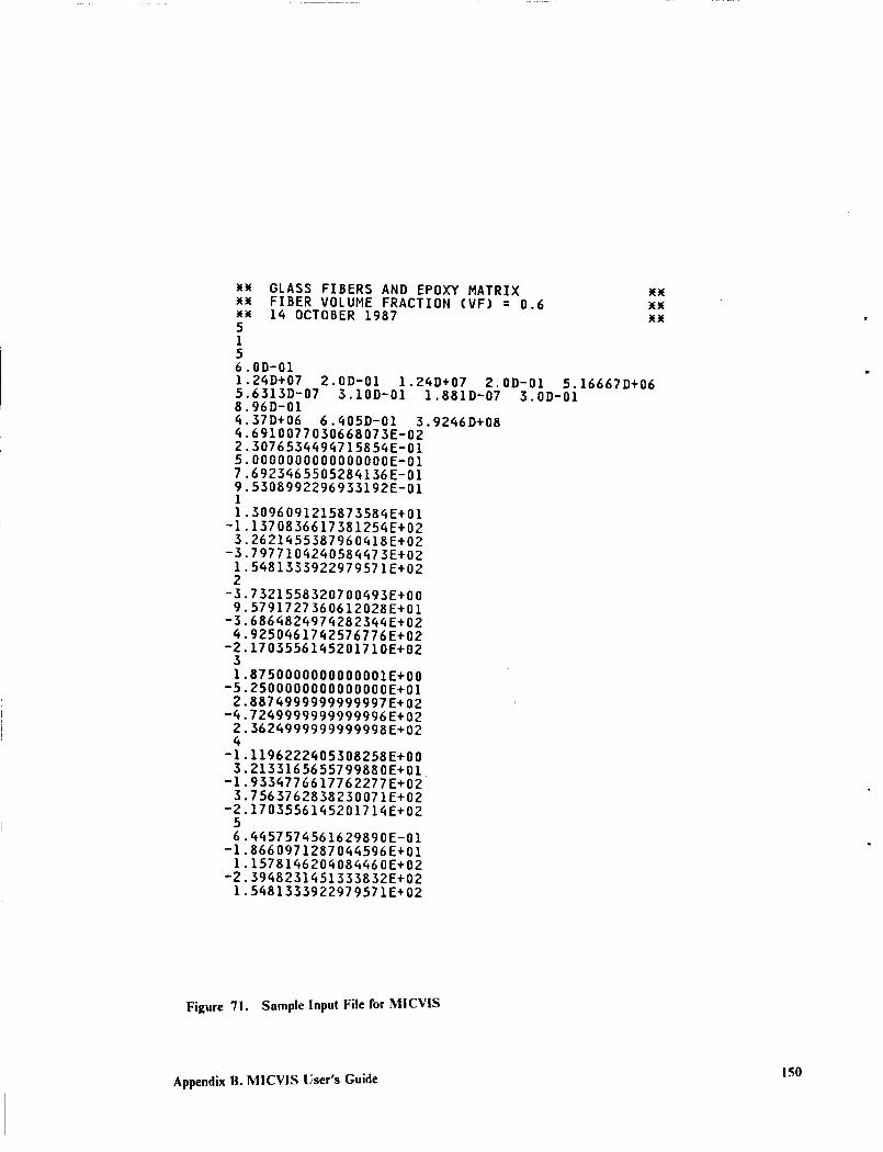
ww GLASS FIBERS AND EPOXY MATRIX_w FIBER VOLUME FRACTION (VF) = 0.6w_ 14 OCTOBER 19875156158

257911.309609121587358qE+01

-I.137083661738125_E+023.2621455387960418E+02

-3.797710q2qO58_75E+021.5_81333922979571E+022

-3.7321558320700_93E+009.5791727360612028E+01

-3.686_82_9742823_E+02_.9250_617_2576776E+02

-2.17035561_SZO171OE+0231.8750000000000001E+00

-5.2500000000000000E+012.887q999999999997E+02

-_.72_9999999999996E÷022.362q999999999998E+02

-1.1196222_05308258E+003.2135165655799880E+01

-l.93G_776617762277E+023.7563762838230071E+02

-2,17035561_520171_E+0256.q_57574561629890E-01

-I.86609712870q_596E+011.15781_620q08qq60E+02

-2.39_8231451333832E+021.Sq81333922979571E+02

.OD-O1

.2_D+07 2.0D-01 1.2qD+07 2.0D-01.6313D-07 3.10D-O1 1.881D-07 3.0D-O1.96D-01.37D+06 6.qOSD-01 3.92_6D+08.6910077030668073E-02.307653_9_71585_E-01.O000000000000000E-01.6923_6550528_136E-01.5308992296933192E-01

3(3(X3()EX

5.16667D+06

Figure '71. Sample Input File for MICVIS

Appendix B. MICVIS User's Guide150

B.3 Output Description

The output comes with a Program Identification Block, a Problem Identification Block, and the

values for the calculated compliances at the given times. A sample output for the Hashin Model

is shown in Figure 72. A U or an L appearing after the compliance value denotes an upper and

lower bound respectively. Figure 73 gives a sample output for the Aboudi Model.


_ MICVIS _w_ HASHIN MODEL wwww VISCOELASTIC CREEP COMPLIANCES ww_w LAPLACE INVERSION BY w_ww THE BELLMAN METHOD ww

ww __w ww_w ww

PROGRAMMED BYROBERT N. YANCEY

OCTOBER 1987w_wwwww_w_wwxxw_wxw_ww_ww_ww_x_w_xwwx__w

www_wwwwwww_wwwwww_www_wwww_w_ww_www_ww_w_wwwww_ww GLASS FIBERS AND EPOXY MATRIX www_ FOUR-PARAMETER MODEL _www FIBER VOLUME FRACTION (VF) = 0.6 ww_ I_ OCTOBER 1987 _

EFFECTIVE CREEP COMPLIANCES IN (I/MSI)

TIME $11 S12 $22U $22L S4qU S44L $66

0.05 0.1228 -.0288 0.1820 0.2261 0.5996 0.4228 0.54650.10 0.1230 -.0288 0.1829 0.2280 0.6049 0.42_3 0.55090.14 0.1231 -.0288 0.1838 0.2299 0.6102 0._256 0.55530.19 0.1232 -.0289 0.18_7 0.2318 0.6153 0.4269 0.55960.24 0.1233 -.0289 0.1855 0.2336 0.6202 0._282 0.56380.26 0.1234 -.0289 0.1859 0.2342 0.6220 0.4287 0.56530.52 0.1239 -.0290 0.1900 0.2429 0.6461 0._3_7 0.58550.69 0.1242 -.0291 0.1923 0.2479 0.6601 0.4380 0.59720.79 0.12_3 -.0291 0.193_ 0.2501 0.6664 0.q396 0.60251.05 0.1246 -.0292 0.1963 0.2563 0.6836 0._35 0.61701.31 0.1249 -.0292 0.1987 0.2616 0.6983 0.4467 0.62931.39 0.1250 -.0293 0.1994 0.2631 0.7026 0._76 0.63291._7 0.1250 -.0293 0.1999 0.26_2 0.7056 0._483 0.635_2.08 0.1254 -.029_ 0.2038 0.2731 0.7306 0.4532 0.65632.77 0.1257 -.0294 0.2066 0.2798 0.7491 0.4565 0.67182.93 0.1257 -.0294 0.2070 0.2806 0.7515 0._569 0.67383.06 0.1258 -.0294 0.2076 0.2822 0.7559 0._575 0.67753.47 0.1258 -.0294 0.2085 0.2842 0.7614 0._585 0.6821_._0 0.1259 -.0295 0.2098 0.2876 0.7708 0.4598 0.68995.87 0.1260 -.0295 0.2111 0.2908 0.7800 0.4611 0.69766.12 0.1260 -.0295 0.2116 0.2920 0.7832 0._615 0.70037.33 0.1261 -.0295 0.2119 0.2927 0.7853 0._617 0.70209.18 0.1261 -.0295 0.2130 0.2955 0.7930 0._629 0.7085

12.24 0.1262 -.0295 0.21_0 0.2981 0.8002 0._6_0 0.714515.30 0.1263 -.0296 0.2150 0.3005 0.8070 0._651 0.7202

Figure 72. Sample Output for ltashin Model


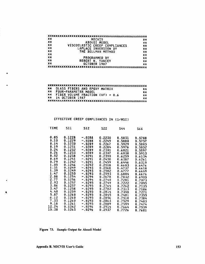
ww MICVIS ww_w ABOUDI MODEL wwww VISCOELASTIC CREEP COMPLIANCES wwxw LAPLACE INVERSION BY ww_w THE BELLMAN METHOD ww

w_ PROGRAMMED BY wwww ROBERT N. YANCEY _w_w OCTOBER 1987 _wwwwww_w_w_www_w_w_ww_www_wwww_wwwwwwww_

_www_wwwww_w_ww_www_w_www_www_wwwww_ww_ GLASS FIBERS AND EPOXY MATRIX __ FOUR-PARAMETER MODEL __w FIBER VOLUME FRACTION (VF) = 0.6 _w_ 14 OCTOBER 1987 ww

EFFECTIVE CREEP COMPLIANCES IN (I/MSI)

TIME 511 512 522 $44 566

0.050.100.140.190.240.260.520.690.791.051,311.391.472 082 772 9_

0647

4 405.876.Z27.339.18

12.2415.30

0.1228 -.0288 0.22300.1229 -.0288 0.22490.1230 -.0289 0.22670.1231 -.0289 0.22840.1232 -.0289 0.23010.1233 -.0289 0.23070.1238 -.0291 0.23900.1241 -.0291 0.24380.1242 -.0291 0.24590.1246 -.0292 0.25180.1249 -.0293 0.25680.1249 -.0293 0.25820.1250 -.0293 0.25930.1254 -.0294 0.26780.1256 -.0294 0.27400.1257 -.0295 0.27490.1257 -.0295 0.27640.1258 -.0295 0,27820.1259 -.0295 0.28140.1260 -.0295 0.28450.1260 -.0295 0.28560.1260 -.0295 0.28630.1261 -.0295 0.28890.1262 -.0296 0.29140.1263 -.0296 0.2937

0.58310.58800.59290.59760.60210.60380.62590.63870.64460.66030.67370.67770.68040.70320.72010.72220.72620.73130 7 3980 74810 75100 75290 75990 76640 7726

0.57080.57570.58050.58520.58970.59130.61340.62610.63190.64760.66100.66490.66760.69050.70730.70950.71350 71860 72710 73550 73840 74030 74740 75390.7601

Figure 73. Sample Output for Aboudi Model

Appendix B. MICV1S User's Guide 153

Appendix C. Elastic Properties

Following are a list of tables showing the composite and bulk resin elastic properties as evaluated

in this study. Also given are tables showing the elastic properties as determined by Milkovich, et

al. [161, Reed, et al. [231, and Fox, et al. 1261. It should be kept in mind that the resin system used

by Reed is slightly different than the resin system used in this study or in Milkovich, et al. [16].

Appendix C. Elastic Properties 154

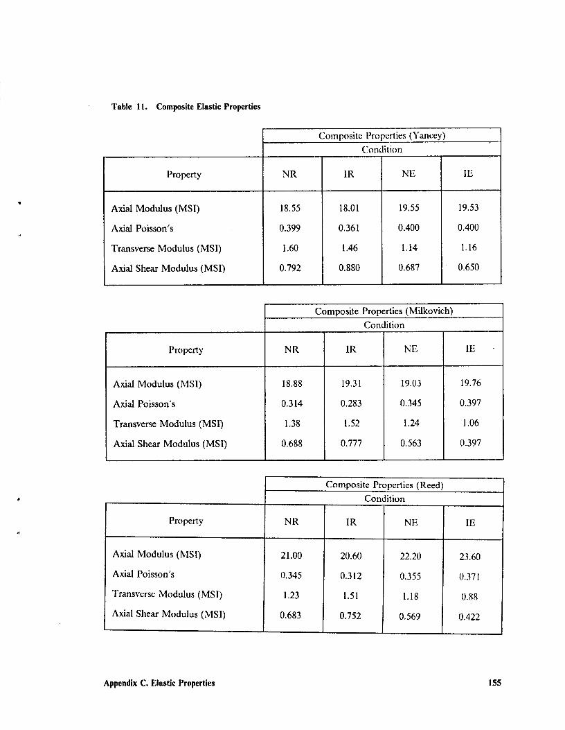
Table II. Composite Elastic Properties

Composite Properties (Yancey)

Property

Axial Modulus (MSI)

Axial Poisson's



NR

18.55

0.399

1.60

0.792

IR

18.01

0.361

1.46

0.880

Condition

NE

19.55

0.400

1.14

0.687

IE

19,53

0.400

1.16

0.650

Property

Axial Modulus (MSI)

Axial Poisson's



NR

18.88

0.314

1.38

0.688

Composite Properties (Milkovich)

Condition

IR NE

19.31 19.03

0.283 0.345

1.52 1.24

0.777 0.563

IE

19.76

0.397

1.06

0.397

Composite Properties (Reed)

Condition

Property

Axial Modulus (MSI)

Axial Poisson's



NR

21.00

0.345

1.23

0.683

IR

20.60

0.312

1.51

0.752

NE

22.20

0.355

1.18

0.569

IE

23.60

0.371

0.88

0.422


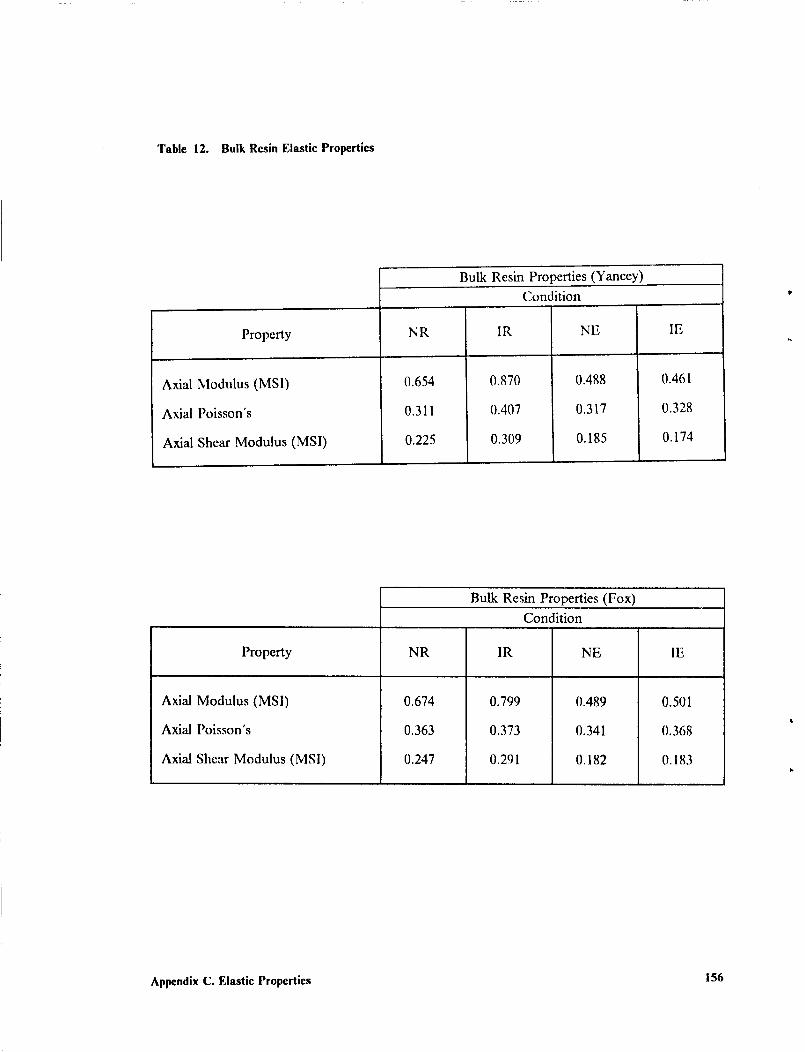
Table 12. Bulk Resin Elastic Properties

Property

Axial Modulus (MSI)

Axial Poisson's


NR

0.654

0.311

0.225

Bulk Resin Properties (Yancey)

Condition

IR NE

0.870 0.488

I).407 0.317

0.309 0.185

IE

0.461

0.328

0.174

Property

Axial Modulus (MSI)

Axial Poisson's


NR

0.674

0.363

0.247

Bulk Resin Properties (Fox)

Condition

IR NE

0.799 0.489

0.373 0.341

0.291 0.182

IE

0.501

0.368

0.183


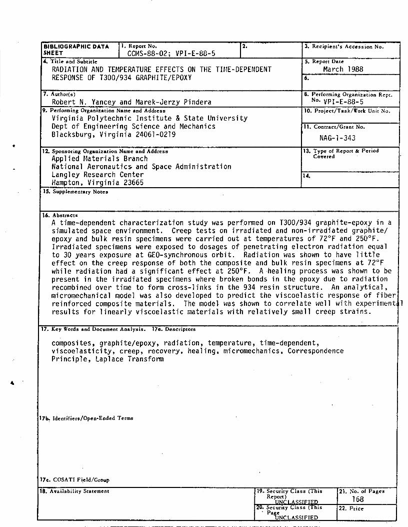
BIBLIOGRAPHIC DATA ] 1. Report No. 12 •SHEET CCMS-88-02; VPI-E-88-5M

4. Title and Subtitle

RADIATION AND TEMPERATURE EFFECTS ON THE TIME-DEPENDENT

RESPONSE OF T300/934 GRAPHITE/EPOXY

7. Author(s)

Robert N. Yancey and Marek-derzy Pindera

9. Performing Organization Name and Address

Virginia Polytechnic Institute & State University

Dept of Engineering Science and Mechanics

Blacksburg, Virginia 24061-0219

12. Sponsoring Organization Name and Address

Applied Materials Branch

National Aeronautics and Space Administration

Langley Research Center

Hampton, Virginia 23665

3. Recipient's Accession No.

5. Report Date !'

March 1988

6.

8. Performing Organization Rept.

No. VPI-E-88-5

10. Project/Task/Work Unit No.

11. Contract/Grant No.

NAG-1-343

13. Type of Report & PeriodCovered

14.

IS. Supplementary Notes

16. Abstracts

A time-dependent characterization study was performed on T300/934 graphite-epoxY in asimulated space environment. Creep tests on irradiated and non-irradiated graphite/

epoxy and bulk resin specimens were carried out at temperatures of 72°F and 250°F.

Irradiated specimens were exposed to dosages of penetrating electron radiation equal

to 30 years exposure at GEO-synchronous orbit. Radiation was shown to have little

effect on the creep response of both the composite and bulk resin specimens at 72°F

while radiation had a significant effect at 250°F. A healing process was shown to be

present in tile irradiated specimens where broken bonds in the epoxy due to radiation

recombined over time to form cross-links in the 934 resin structure. An analytical,

micromechanical model was also developed to predict the viscoelastic response of fiber

reinforced composite materials. The mode] was shown to correlate well with experiment,

results for linearly viscoelastic materials with relatively small creep strains.

17. Key Words and Document Analysis. 17a. Descriptors

composites, graphite/epoxy, radiation, temperature, time-dependent,

viscoelasticity, creep, recovery, healing, micromechanics, Correspondence

Principle, Laplace Transform

17b. Identifiers/Open-Ended Terms

17¢. COSATI Field/Group

18. Availability Statement

19.. Security Class (ThisReport)UNCLASSIFIED

20. Security Class (This• Page

-UNCLASSIFIED

21. No. of Pages168

22. Price

Documents

CENTER FOR CI,)MPOSITE MATERIALS AND …")MPOSITE MATERIALS AND STRUCTURES ... _I_0/9311 GI_&I?tlI_I_/RBCII lntslil lte_o_t ... A time-dependent characterization study was performed