CENTER FOR MACHINE PERCEPTION Eye-Blink Detection Using ... · Title of Diploma Thesis : Eye -Blink Detection Using Facial Landmarks . Guidelines: 1. Propose an eye- blink detection

CENTER FOR

MACHINE PERCEPTION

CZECH TECHNICAL

UNIVERSITY IN PRAGUE

DIPLOMATHESIS

ISSN

1213-2365

Eye-Blink Detection Using

Facial LandmarksTereza Soukupova

[email protected]

CTU–CMP–2016–05

May 26, 2016

Available at

ftp://cmp.felk.cvut.cz/pub/cmp/articles/cech/Soukupova-TR-2016-05.pdf

Thesis Advisor: Jan Cech

The research was supported by CTU student grant

SGS15/155/OHK3/2T/13.

Research Reports of CMP, Czech Technical University in Prague, No. 5, 2016

Published by

Center for Machine Perception, Department of Cybernetics

Faculty of Electrical Engineering, Czech Technical University

Technicka 2, 166 27 Prague 6, Czech Republic

fax +420 2 2435 7385, phone +420 2 2435 7637, www: http://cmp.felk.cvut.cz

Eye-Blink Detection Using

Facial Landmarks

Tereza Soukupova

May 26, 2016

Czech Technical University in Prague Faculty of Electrical Engineering

Department of Cybernetics

DIPLOMA THESIS ASSIGNMENT

Student: Bc. Tereza S o u k u p o v á

Study programme: Open Informatics

Specialisation: Computer Vision and Image Processing

Title of Diploma Thesis: Eye-Blink Detection Using Facial Landmarks

Guidelines: 1. Propose an eye-blink detection algorithm that uses facial landmarks as an input. 2. Evaluate the proposed detector quantitatively based on the ground-truth dataset. Study the detector sensitivity on the image/video quality (especially on face resolution, video frame rate, head pose, or partial occlusions). 3. Prepare a demonstration of the proposed eye-blink detector and consider an application in the context of e.g., Human-Computer Interface, attention monitoring, drowsiness detection, etc. Bibliography/Sources: [1] X. Xiong and F. De la Torre, "Supervised descent methods and its applications to face alignment", in Proc. Conference on Computer Vision and Pattern Recognition, 2013. [2] A. Asthana, S. Zafeoriou, S. Cheng, and M. Pantic, "Incremental face alignment in the wild", in Proc. Conference on Computer Vision and Pattern Recognition, 2014. [3] J. Cech, V. Franc, M. Uricar, and J. Matas. Multi-view facial landmark detection by using a 3D shape model. Image and Vision Computing, 2016. In Press. [4] T. Drutarovsky and A. Fogelton, "Eye blink detection using variance of motion vectors", in Computer Vision - ECCV 2014 Workshops, 2014. [5] G. Pan, L. Sun, Z. Wu, and S. Lao, "Eyeblink-based anti-spoofing in face recognition from a generic webcamera", in ICCV, 2007.

Diploma Thesis Supervisor: Ing. Jan Čech, Ph.D.

Valid until: the end of the summer semester of academic year 2016/2017

L.S.

prof. Dr. Ing. Jan Kybic Head of Department

prof. Ing. Pavel Ripka, CSc. Dean

Prague, January 8, 2016

Acknowledgment

I would like to thank Ing. Jan Cech, Ph.D. for his guidance, patience, willingness and

assistance during the writing of my thesis. I also thank prof. Ing. Jirı Matas, Ph.D.

for his advice.

Author statement for undergraduate thesis

I declare that the presented work was developed independently and that I have listed

all sources of information used within it in accordance with the methodical instructions

for observing the ethical principles in the preparation of university theses.

Prague, 27 May 2016 ...................................

iii

Abstract

A real-time algorithm to detect eye blinks in a video sequence from a standard camera

is proposed. Recent landmark detectors, trained on in-the-wild datasets exhibit ex-

cellent robustness against face resolution, varying illumination and facial expressions.

We show that the landmarks are detected precisely enough to reliably estimate the level

of the eye openness. The proposed algorithm therefore estimates the facial landmark

positions, extracts a single scalar quantity – eye aspect ratio (EAR) – characterizing

the eye openness in each frame. Finally, blinks are detected either by an SVM classifier

detecting eye blinks as a pattern of EAR values in a short temporal window or by

hidden Markov model that estimates the eye states followed by a simple state machine

recognizing the blinks according to the eye closure lengths. The proposed algorithm

has comparable results with the state-of-the-art methods on three standard datasets.

Keywords

Eyes, eye blink, eye blink detector, face, landmarks, eye aspect ratio, EAR, SVM,

HMM.

iv

Abstrakt

Prace se zabyva detekcı mrkanı ocı ve videozaznamu porızenem standardnı webkamerou.

V nedavne dobe byly predstaveny oblicejove detektory na detekci a sledovanı vyznamnych

bodu v obliceji. Tyto detektory dosahujı vybornych vysledku a jsou velmi robustnı vuci

ruznorodemu osvetlenı, rozlisenı obliceje v obraze a vyrazu v tvari. Ukazeme, ze s po-

mocı techto oblicejovych detektoru umıme spolehlive odhadnout mıru otevrenosti oka.

Algoritmus tedy nejdrıve odhadne vyznamne body v obliceji, potom z techto bodu

vypocıta skalarnı hodnotu jako pomer vysky a sırky oka (eye aspect ratio EAR), ktera

charakterizuje mıru otevrenosti oka v kazdem snımku videosekvence. Mrknutı jsou

pak detekovana bud SVM klasifikatorem, ktery se naucı charakteristicky vzor mrknutı

z EAR hodnot v kratkem casovem useku a nebo jsou mrknutı detekovana skrytym

Markovovym modelem, ktery v kazdem snımku urcı, zda je oko zavrene nebo otevrene,

a na zaklade delky mrknutı pak stavovy automat rozpozna ktera zavrenı ocı znamenala

mrknutı. Navrhovane metody pracujı v realnem case a dosahujı srovnatelnych vysledku

se state-of-the-art.

Klıcova slova

Oci, mrkanı, detektor mrkanı, oblicej, vyznamne body v obliceji, EAR, SVM, HMM.

v

Contents

1 Introduction 2

2 Eye Blinks 4

2.1 What is eye blinking? . . . . . . . . . . . . . . . . . . . . . . . . . . . . 4

2.1.1 Parameters of blinks . . . . . . . . . . . . . . . . . . . . . . . . . 4

3 Related work 5

3.1 State-of-the-art of blink detectors . . . . . . . . . . . . . . . . . . . . . . 5

3.2 Drowsiness detection approaches . . . . . . . . . . . . . . . . . . . . . . 9

4 Proposed method 11

4.1 Eye blink detection using Support Vector Machine classifier (EAR SVM) 11

4.2 Eye blink detection using Hidden Markov Model (EAR adaptive HMM) 13

4.2.1 Detecting eye states by Hidden Markov Model . . . . . . . . . . 14

4.2.2 Detecting blinks via state machine . . . . . . . . . . . . . . . . . 15

4.2.3 Adaptation of HMM in time . . . . . . . . . . . . . . . . . . . . 15

5 Experiments and datasets 17

5.1 Accuracy of landmark detectors . . . . . . . . . . . . . . . . . . . . . . . 17

5.2 Eye blink detector evaluation . . . . . . . . . . . . . . . . . . . . . . . . 20

5.2.1 Datasets for blink detection . . . . . . . . . . . . . . . . . . . . . 21

ZJU . . . . . . . . . . . . . . . . . . . . . . . . . . . . . . . . . . 21

Eyeblink8 . . . . . . . . . . . . . . . . . . . . . . . . . . . . . . . 21

The Silesian eye blink dataset . . . . . . . . . . . . . . . . . . . . 22

5.2.2 EAR SVM eye blink detector . . . . . . . . . . . . . . . . . . . . 22

5.2.3 EAR adaptive HMM eye blink detector . . . . . . . . . . . . . . 25

5.2.4 Computation of blink statistics . . . . . . . . . . . . . . . . . . . 27

Blink frequency . . . . . . . . . . . . . . . . . . . . . . . . . . . . 27

Blink duration . . . . . . . . . . . . . . . . . . . . . . . . . . . . 27

Blink amplitude . . . . . . . . . . . . . . . . . . . . . . . . . . . 30

5.2.5 Experiments on sensitivity of proposed blink detectors . . . . . . 31

Change of resolution . . . . . . . . . . . . . . . . . . . . . . . . . 31

Change of frame rate . . . . . . . . . . . . . . . . . . . . . . . . . 34

6 Eye blink detector application 36

7 Implementation details 39

8 Conclusion 40

Bibliography 41

1

1 Introduction

Detecting eye blinks is important for instance in systems that monitor a human operator

vigilance, e.g. driver drowsiness [1], in systems that warn a computer user staring at

the screen without blinking for a long time to prevent the dry eye and the computer

vision syndromes [2, 3], in human computer interfaces that ease communication for

disabled people [4], or for anti-spoofing protection in face recognition systems [5].

Many methods have been proposed to automatically detect eye blinks in a video

sequence. The methods are more detailed in Sec. 3.1. Their major drawback is that

they usually implicitly impose too strong requirements on the setup, in the sense of

a relative face-camera pose (head orientation), image resolution, illumination, motion

dynamics, etc. Especially the heuristic methods that use raw image intensity are likely

to be very sensitive despite their real-time performance.

However nowadays, robust real-time facial landmark detectors [6, 7, 8] that capture

most of the characteristic points on a human face image, including eye corners and

eyelids, are available. Most of the state-of-the-art landmark detectors formulate a re-

gression problem, where a mapping from an image into landmark positions or into other

landmark parametrization is learned. These modern landmark detectors are trained on

in-the-wild datasets and they are thus robust to varying illumination, various facial ex-

pressions, and moderate non-frontal head rotations. An average error of the landmark

localization of a state-of-the-art detector is usually below five percent of the inter-ocular

distance.

Therefore, we propose a simple but efficient algorithm to detect eye blinks by using

a recent facial landmark detector. A single scalar quantity that reflects a level of the eye

openness is derived from the landmarks. Finally, having a per-frame sequence of the

eye openness estimates, the eye blinks are detected by two proposed methods. The first

one finds blinks by an SVM classifier that is trained on examples of blinking and non-

blinking patterns. The second method is unsupervised. It learns a Hidden Markov

Model to estimate eye states. Eye blinks are then detected via simple state machine

according to the blink duration. The blink detectors are evaluated on three standard

blink datasets with ground-truth annotations.

A small study to measure blink properties such as frequency over time and duration

is carried out. These characteristics are important to determine a degree of drowsiness.

We define a drowsiness index as a function of blink frequency and blink duration. Fi-

nally the blink detection is applied and an experiment measuring a subject drowsiness

during a day while working on a laptop is presented.

2

A structure of the work is following. You can read about eye blinking from physiolog-

ical point of view in Chapter 2. Chapter 3 presents related work. Chapter 4 describes

the proposed methods for blink detection. Experiments and testing of the proposed

algorithms are described in Chapter 5. You can find our blink application determin-

ing drowsiness while using laptop in Chapter 6. There are implementation details in

Chapter 7. Chapter 8 concludes the work.

3

2 Eye Blinks

2.1 What is eye blinking?

Eye blinking is partly subconscious fast closing and reopening of the eyelid. There are

multiple muscles involved in eye blinking. Two main muscles are orbicularis oculi and

levator palpebrae superioris that control the eye closing and opening.

The main purpose of eye blinking is to moisten an eye cornea. It also cleans the eye

cornea when eyelashes do not capture all the dust and a dirt gets into the eye.

There are two types of unconscious blinking. The spontaneous blinking is done with-

out any obvious external stimulus. It happens while breathing or digesting. The second

type of involuntary blinking is called the reflex blinking. It is caused by contact with

the cornea, fast visual change of light in front of the eye, sudden presence of near object

or by a loud noise. Another type of blinking is the voluntary blinking which is invoked

consciously under the control of the individual.

2.1.1 Parameters of blinks

There are two main parameters of blinking: frequency and duration. Average frequency

of blinking of an adult is 15-20 blinks/min but there are only 2-4 blinks/min physio-

logically needed. Children have lower blink rate. Newborns even blink only 2× per

minute. Interestingly, women using oral contraceptives blink 32% more often than

other women [9]. The rate of spontaneous blinking can be increased by a strong wind,

dry air conditions or by emotional situations. On the other hand, when the eyes are

focused on an object for longer time (e.g. reading), the blink rate decreases to about

3-4 blinks/min.

Work [10] publishes a hypothesis that the blink frequency is increased by negative

mood, stress, nervousness, fatigue, negative emotions, pain, boredom. On the other

hand the frequency is decreased in positive states while relaxing, having pleasant feeling,

after successful problem solving and also while reading and having greater attention.

The duration of blinking depends on an individual, usually it is about 100-400 ms.

The reflex blinking is faster then the spontaneous. Blink frequency and duration can be

affected by relative humidity, temperature, brightness or by fatigue, disease or physical

activity.

4

3 Related work

3.1 State-of-the-art of blink detectors

Many of different methods have been developed for blink detection. We can divide

them into several categories according to requirements on a setup and their performance.

The output can be either open/closed eye recognition or a blink detection. The methods

are divided as intrusive and non-intrusive. The intrusive methods require a special

hardware on setup such as electrodes placed along the scalp to measure EOG [11],

Doppler sensor [12, 13] or glasses with a special close-up cameras observing the eyes [14].

The non-intrusive optical methods can also use a special hardware such as illuminators

or infrared cameras [15, 16, 17], but many modern approaches aim to have non-intrusive

systems relying on a standard remote camera only.

The second group consists of non-intrusive vision-based techniques using only an RGB

camera. They use either single image characteristics or they use several subsequent

frames from a video sequence to detect a motion. They usually have three stages:

a face detection, an eye region detection and a blink detection. Viola-Jones algorithm

is mostly used for face detection.

The single image processing approaches are based e.g. on skin color segmenta-

tion [18], edge detection, a parametric model fitting to find the eyelids [19], or active

shape models [20]. In [21] vertical intensity projections are used. The intensities

are summed in a row and while supposing that eyebrow and the iris area are darker

than skin. So, there are two projections minima and one maximum between them, see

Fig. 3.1. A change of the projection curve during blinking is investigated. A method [22]

is similar in spirit of using pixel intensities but histograms instead of projections are

used. Another method [1] assumes that an open eye is horizontally symmetric, whereas

a closed eye is not. The eye region is horizontally divided into upper and lower halves.

On the basis of the cumulative sum of the intensities open and closed eye patterns are

compared. There is a combination of two methods in [23]. An eye region to binary

image is converted and morphological closure is done, see Fig. 3.2. Two features are

computed: a cumulative difference of black pixels in successive images and a ratio of

height to width of eye. An SVM on the basis of the two features mentioned previously

is used to recognize if an eye is open or closed. Most of these methods are sensitive to

illumination.

Another method for blink detection is based on template matching [24, 25, 26, 27].

The templates with open and/or closed eyes are learned and normalized cross correlation

5

3 Related work

Figure 3.1 An example of intensity vertical projections from a method described in [21].

Figure 3.2 An example of binarized eye regions described in method [23].

coefficient R is computed for an eye region of each image:

R(x, y) =

∑x′,y′(T (x′, y′)− I(x+ x′, y + y′))2√∑

x′,y′ T (x′, y′)2∑

x′,y′ I(x+ x′, y + y′)2, (3.1)

where I is original image, T is template image and x and y are pixel coordinates.

The correlation score is then compared for open and closed eye template. In [25],

a correlation only with open eye template is computed and a change of R in time is

analyzed. A blink starts if two consecutive frames have R value lower then predefined

threshold TL and ends if two consecutive frames have correlation coefficient greater

than threshold TH. The goal is to detect voluntary blinks which are defined as blinks

longer than 250 ms and shorter than 2 s. They do not have offline preprocessed template

in [26] but the template is learned online at the beginning of a sequence. The examples

of open eye templates can be seen in Fig. 3.3.

Figure 3.3 Open eye templates. Image taken from [26].

6

3.1 State-of-the-art of blink detectors

Figure 3.4 An example of facial and eyelids motion more described in [32].

There are many motion based methods which need two or more consecutive frames

for frame differencing [28, 29]. A difference of two consecutive frames and application

of morphological operations is done in paper [30]. A motion of eyelids is detected if

a sum of intensities of the subtraction is greater than a given threshold. However, it is

not known if an eye is open or closed after the motion. Thus, the frames differencing

with analysis of the vertical and horizontal projections in binary image are combined.

The methods using optical flow [31, 2] usually tend to estimate dominant movement

direction and magnitude. A methods using similar motion analysis is described in [32].

A movement of a whole face must be distinguished and subtracted to capture the resid-

ual movement of the eyelids, see Fig. 3.4. Another method using motion analysis can be

found in [33]. A histogram of oriented gradients is used for blink detection. A paper [34]

combines a spatial and temporal derivatives which represent motion between frames.

Only motion vectors in vertical direction are analyzed. Another motion approach is

described in work [3]. There are about 255 KLT trackers in an eye region divided into

3 × 3 cells. A local average motion is computed from KLT trackers belonging to each

cell. The eye blink is detected by a state machine if a downward movement occurs and

the upward movement is present no later than 150 ms. A workflow of the proposed eye

blink detector is shown in Fig. 3.5. In [35] a similar approach is used. It is supposed,

that all the motion vectors for each pixel are similar to each other in magnitude and

orientation during head movement in contrast with the eye blink movement where mo-

tion vectors differ. So a state machine is set up and a blink is detected based on mean

values and standard deviations of vertical components of vector motions. The state

machine also takes a time spent in a closed state into account.

There are two similar methods to ours using facial landmarks. A paper [20] presents

a method where Active Shape Model is used to obtain 98 facial landmarks, 8 of them

7

3 Related work

Figure 3.5 An example of motion based method described in work [3].

Figure 3.6 Left: the arrows illustrate distances for computing eye aperture a(t). Right: a(t)

for several frames with 4 blinks detected. The quartiles Q1, Q2 and Q3 and values A0, A80

and A1000 are depicted. Whole method is described in [20].

are for each of the eye to approximate an eye shape. The aperture a(t) of the eye at

time t is computed as average distance between vertically corresponding landmarks.

A reference level A0 is set as a median of a(t). The values a(t) are considered to be

outliers if they are lower than heuristic threshold Aout = Q3 − 1.5(Q1 − Q3), where

Q1, Q2 and Q3 are quartiles of a(t). The average of peak values of outliers is denoted

as A100. They are interested of measuring the PERCLOS [36] metric which is defined

as a time that the eyes are closed 80% or more. The threshold denoting that eyes are at

least 80% closed is computed as A80 = A0−0.8(A0−A100). The value A80 is computed

iteratively because some blinks can be discarded or added. The situation is depicted

in Fig. 3.6. This approach is suitable only for offline processing because it needs whole

video sequence for parameter estimation.

The second system [37] using Active Shape Model is based on eye contour extraction

represented by 16 landmarks. Eye openness degree is computed in a similar way as

8

3.2 Drowsiness detection approaches

Figure 3.7 Eye openness degree is computed as a ratio between height of the eyes and a distance

between eyes in [37].

we do but a ratio of average height of eyes to a distance between eyes is used, see

Fig. 3.7. Eye blink is detected if the eye openness degree changes from larger than

threshold thl = 0.12 to smaller than ths = 0.02. This is a baseline method which do

not solve many problems in videos in-the-wild. The method does not admit that the

thresholds may be different for different people. It also does not take facial expressions

into account. The average time to process one frame is about 140 ms so it runs real-time

only for videos with frame rate lower than 7 fps.

The listed methods have different limitations. They are mostly sensitive to image

resolution, illumination, or head pose, etc. or their computational cost is high. Many

of them do not take into account a fact that it does not generally hold that eye closing

always means the eye blinking. We note that many eye blink detectors only distinguish

between open and closed states of the eye but they do not detect blinks over time at all.

3.2 Drowsiness detection approaches

One of the most frequent application of blink detection is to detect a subject drowsiness.

E.g. it may be used to alert a car driver when he or she is too tired. A standard indicator

of drowsiness is PERCLOS [36]: ”Proportion of time that the eyes are 80% to 100%

closed.” Papers [38, 19, 39] estimate drowsiness using PERCLOS. Another common

approach is to measure drowsiness according to the blink frequency [40, 41, 39] or

according to the blink duration. In [1] blinks are divided according to the duration to

3 groups: awake (blink duration shorter than 400 ms), drowsy (blink duration between

400 ms and 800 ms) and sleepy (blink duration longer than 800 ms). A drowsiness

is detected when the eyes remain closed for two or more seconds in [42]. A complex

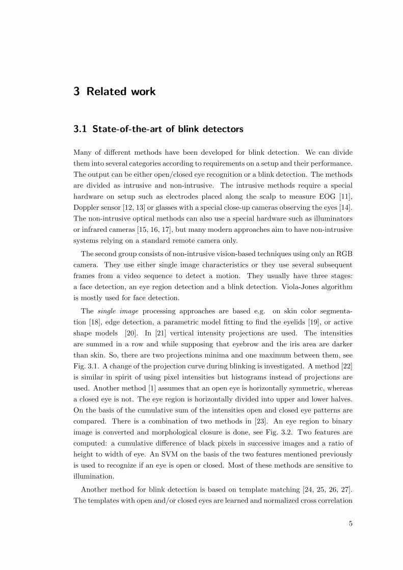
algorithm detecting a subject fatigue is described in [43]. A fatigue is regarded as the

result of many variables such as health, sleep history, workload or weather. A Bayesian

Network model using together observations such as PERCLOS, percentage of saccade

eye movement, eyelid and head movement, etc. is constructed. All parameters used are

shown in Fig. 3.8.

9

3 Related work

Figure 3.8 A fatigue Bayesian Network model described in paper [43].

10

4 Proposed method

The eye blink is a fast closing and reopening of a human eye. Each individual has a little

bit different pattern of blinks. The pattern differs in the speed of eyelid movement, in

a degree of squeezing the eyes and in a blink duration. The eye blink lasts approximately

100-400 ms.

We propose to exploit state-of-the-art facial landmark detectors to localize the eyes

and eyelid contours. From the landmarks detected in the image with face, we derive

the eye aspect ratio (EAR) that is used as an estimate of the eye openness state. Since

the per-frame EAR may not necessarily recognize the eye blinks reliably, a classifier

that takes a larger temporal window of a frame into account is trained.

For every video frame, the eye landmarks are detected. The eye aspect ratio (EAR)

between height and width of the eye is computed.

EAR =‖p2 − p6‖+ ‖p3 − p5‖

2‖p1 − p4‖, (4.1)

where p1, . . . , p6 are the 2D landmark locations, depicted in Fig. 4.1.

The EAR is mostly constant when an eye is open and is getting close to zero while

closing the eye. It is partially person and head pose insensitive. Eye aspect ratio of the

open eye has a small variance among individuals and it is fully invariant to a uniform

scaling of the image and in-plane rotation of the face. Since eye blinking is performed

by both eyes synchronously, the EAR of both eyes is averaged. An example of an EAR

signal over several frames in the video sequence is shown in Fig. 4.1, 5.8, 5.10, 5.14, 5.15.

Two approaches are proposed in the thesis. The first one is supervised thus training

process is needed. An SVM classifier is learned on training dataset. The second method

is unsupervised. The blinking is modelled by Hidden Markov Model.

4.1 Eye blink detection using Support Vector Machine

classifier (EAR SVM)

It generally does not hold that low value of the EAR means that a person is blinking.

A low value of the EAR may occur when a subject closes his/her eyes intentionally

for a longer time or performs a facial expression, yawning, etc., or the EAR captures

a short random fluctuation of the landmarks.

Therefore, we propose a classifier that takes a larger temporal window of a frame as

an input. Due to a normally blink length being from 100 ms to 400 ms, we decided

that approximately 430 ms can have a significant impact on a blink detection. Further

11

4 Proposed method

Figure 4.1 Open and closed eyes with landmarks pi automatically detected by [7]. The eye

aspect ratio EAR in Eq. (4.1) plotted for several frames of a video sequence. A single blink

is present.

Figure 4.2 The eye aspect ratio EAR in Eq. (4.1) plotted for several frames of a video sequence.

A single blink is present. A red box demonstrates the scanning time window.

values are given for 30fps videos. Thus, for example having 30fps video, for each frame

a 13-dimensional feature is gathered by concatenating the EARs of its ±6 neighboring

frames, see Fig. 4.2.

A linear SVM classifier (called EAR SVM) is trained from manually annotated se-

quences. Positive examples are collected as ground-truth blinks, while the negatives are

those that are sampled from parts of the videos where no blink occurs, with 5 frames

spacing. Additionally, to avoid only eye closing or only eye opening being detected

as a positive blink, the starts and ends of the ground-truth blinks are considered as

negatives exampled for training the SVM classifier.

While testing, a classifier is executed in a scanning-window fashion. A 13-dimensional

feature is computed and classified by EAR SVM for each frame except the beginning

12

4.2 Eye blink detection using Hidden Markov Model (EAR adaptive HMM)

and ending of a video sequence. The values are proportionately recalculated for different

frame rates than 30 fps. Proposed algorithm runs online, it means that the blink is

detected immediately after the blink’s end.

4.2 Eye blink detection using Hidden Markov Model (EAR

adaptive HMM)

The eye blink detection method using SVM described in section 4.1 has several limita-

tions. It is impossible to measure a duration of an eye blink using EAR SVM classifier

and it cannot determine longer eye closures. The classifier also needs a lot of het-

erogeneous annotated data for training. The model is generic which means that it is

computed only once and remains the same for all the testing data. The model is not

adapted to a specific person. This may result in a failure because blink lengths, closure

amplitudes and speed of eyelid movements differ for each individual so the values of

EAR over time in Eq. (4.1) are diverse. These characteristics are even non-stationary.

It means that they may change over time for a single person. That is the main moti-

vation to use other model which is adaptive to a person and time.

We assume that the sequence of observations of the eye aspect ratio values over time

is a Markov process where the states of the eye are not directly visible. Thus it is

modeled by hidden Markov model (HMM) λ [44, 45, 46]:

λ = (A,B, π) (4.2)

where A is the transition matrix, B is the emission matrix and π is the matrix with

initial probabilities. The variables A, B and π are described further.

In general for HMM, there are three main problems:

1. The first is the evaluation problem. The task is to determine the likelihood of a se-

quence given the model parametres.

2. The second problem is the decoding. The task is to find the most likely sequence of

the hidden states generating the observations when the model parametres are known.

This problem is solved by Viterbi algorithm [47].

3. The third problem is learning the model. The task is to estimate the model parame-

ters that maximize the probability of the observed sequence. This problem is solved

Baum-Welch algorithm [44, 46].

The proposed eye blink detection approach using HMM consists of two stages. In

the first one it is decided in which of two states eyes are (open or closed eye states)

and in the second stage, the eye blinks are determined according to eye closure length

using a simple state machine. Finally, an adaptation mechanism to capture the non-

stationarity and personalisation is carried out.

13

4 Proposed method

4.2.1 Detecting eye states by Hidden Markov Model

The Hidden Markov Model λ = (A,B, π) is specified by a set of hidden (unobservable)

states S. There are only two states in our case. The first state stands for open eye and

the second for closed eye:

S = {s1, s2} = {open, closed} (4.3)

We have a state sequence Q of length T which is a number of frames in a video sequence:

Q = {q1, q2, . . . , qT }. (4.4)

and corresponding observation sequence O:

O = {o1, o2, . . . , oT }, (4.5)

the observations ot are directly the values of EAR (4.1) for each frame. The initial

probabilities of states are determined by matrix π = [πi], where:

πi = P (q1 = si), (4.6)

for states i ∈ {1, 2}. The model is also described by a time independent transition

matrix A = [aij ] which stores the probabilities of one state being followed by another

state:

aij = P (qt = sj |qt−1 = si) (4.7)

for i ∈ {1, 2}, j ∈ {1, 2} and t ∈ {2, . . . T}. The emissions B = [bi(ot)] describe the

probability of a particular observation ot at time t for state i:

bi(ot) = p(ot|qt = si) (4.8)

for i ∈ {1, 2} and t ∈ {1, . . . T}. The emission probabilities B can be either discrete

or continuous. It is more advantageous to use continuous emissions for our purpose.

We suppose that the observation ot for open and closed eye can be modeled by the

Gaussian model:

bi(ot) = N (µi, σ2i ) (4.9)

for i ∈ {1, 2} and t ∈ {1, . . . T}, with mean values µi, and variance σ2i .

HMM parameters need to be estimated. These are transition matrix A between

states, prior probabilities of states π and two means and standard deviations to get

emission probabilities B in Fig. 4.3 modeled by Gaussian distributions. The parameters

are learned in an unsupervised fashion by observing a short sequence of EAR values.

This is estimated by Baum-Welch algorithm which is in fact a kind of Expectation

Maximization algorithm [48]. Maximum likelihood estimate is found by a local iterative

algorithm. An initialization is therefore needed. Having learned the model parameters,

the hidden states are estimated for each video frame by Viterbi [47] algorithm using

the dynamic programming to find the highest score over the sequence.

14

4.2 Eye blink detection using Hidden Markov Model (EAR adaptive HMM)

Figure 4.3 There are EAR values from Eq. (4.1) plotted for several frames of a video sequence

by blue line with a single blink present (left). The corresponding normalized histogram of

EARs. Green and red lines show fitted Gaussians (right).

4.2.2 Detecting blinks via state machine

The algorithm proposed in 4.2.1 only distinguishes between open and closed eyes. Once

the eye states are estimated the eye blinks are detected by a simple state machine which

decides if the eye closure detected by the HMM is eye blinking according to the length

of the closure. The average eye blink duration is between 60 ms to 700 ms according to

the annotated datasets. Thus we consider closures of length between 60 ms and 700 ms

being blinks.

4.2.3 Adaptation of HMM in time

The testing process is initialized with a generic model parameters learned from an anno-

tated training dataset with ground-truth. The generic transition matrix is determined

by relative frequencies and Gaussian distributions are fitted having the blink/non-blink

labels. The generic model parameters are the same for all the testing videos and are

learned only once. They are used only for the initialization of a model of each tested

sequence and further the algorithm using adaptation is unsupervised. The parameters

of the HMM are then repeatedly reestimated in time intervals I to adapt the model to

a specific person. Subsequent model estimation is initialized by the previous solution.

For new estimation only the subsequence of size S of the EAR values is used as an input

for Baum-Welch algorithm.

The current parameters are then computed as a convex combination of several last

estimates with exponential weights wt. Thus more recent estimates have higher weights.

The weights are normalized to sum up to one. The estimates older then learning time

L are forgotten:

wt =e

t2∑L

It=1 e

t2

, (4.10)

15

4 Proposed method

Figure 4.4 The eye aspect ratio EAR in Eq. (4.1) plotted for several frames of a video sequence

by blue line. The black points show the weights wt of models estimated in time t. Red line is

the time L of remembering previous models. Green line shows the size of subsequence S of

EARs used for computation of new model and dotted black lines show intervals I how often

the new model is computed.

where t = 1, . . . , LI . Therefore the parameters of the HMM are iteratively adapting to be

person and time period specific. Between intervals of reestimations of the parameters,

the last calculated model for decoding is used.

The subsequence size S must be large enough to include whole blink plus some

surroundings and simultaneously it must be small enough to quickly adapt the model

to a change and do not make mistake on transitions, e.g. when a subject starts squeezing

its eyes while smiling or when an illumination condition has changed. The time interval

I of model reestimations must be long enough to be able to capture the non-stationarity.

The situation is depicted in Fig. 4.4.

The parameters of the model are not recomputed in a case that no eye state change is

present. It is recognized heuristically by the difference between the lowest and the high-

est value of the EAR in the subsequence. The difference is not higher than threshold D.

If this happens, we do not reestimate whole the model by Baum-Welch algorithm. We

only fit one Gaussian distribution. Due to the mean of the Gaussian we determine if

it belongs to open or closed eye state. To complete the model λt at time t the generic

values are used for the second Gaussian distribution and the rest of the hidden Markov

model parameters remains the same.

16

5 Experiments and datasets

Two types of experiments were carried out: the experiments that measure accuracy

of the landmark detectors, see Sec. 5.1, and the experiments that evaluate performance

of the whole eye blink detection algorithms, see Sec 5.2.

5.1 Accuracy of landmark detectors

To evaluate accuracy of tested landmark detectors, we used the 300-VW dataset [49].

It is a dataset containing 50 videos where each frame has associated a precise annotation

of facial landmarks. The videos are “in-the-wild”, mostly recorded from a TV.

The purpose of the following tests is to demonstrate that recent landmark detectors

are particularly robust and precise in detecting eyes, i.e. the eye-corners and contour

of the eyelids. Therefore we prepared a dataset, a subset of the 300-VW, containing

sample images with both open and closed eyes. More precisely, having the ground-truth

landmark annotation, we sorted the frames of each of the 50 videos by the eye aspect

ratio (EAR in Eq. (4.1)) and took 10 frames of the highest ratio (eyes wide open), 10

frames of the lowest ratio (mostly eyes tightly shut) and 10 frames sampled randomly.

This way we collected 1500 images. Moreover, all the images were later subsampled

(successively 10 times by factor 0.75) in order to evaluate accuracy of tested detectors

on small face images.

Two state-of-the-art landmark detectors were tested: Chehra [7] and Intraface [6].

Both run in real-time1. Samples from the dataset are shown in Fig. 5.1. Notice that

faces are not always frontal to the camera, the expression is not always neutral, people

are often speaking emotionally or smiling, etc. Sometimes people wear glasses or hair

may occasionally partially occlude one of the eyes. Both detectors perform generally

well, but the Intraface is more robust to very small face images, sometimes at impressive

extent as shown in Fig. 5.1.

Quantitatively, the accuracy of the landmark detection for a face image is measured

by the average relative landmark localization error, defined as usually

ε =100

ξN

N∑i=1

||xi − xi||2, (5.1)

where xi is the ground-truth location of landmark i in the image, xi is an estimated

landmark location provided by a detector, N is a number of landmarks and normal-

ization factor ξ is the inter-ocular distance (IOD), i.e. Euclidean distance between eye

centers in the image.

1Intraface runs in 50 Hz on a standard laptop.

17


Chehra

Intraface

Chehra

Intraface

Chehra

Intraface

Chehra

Intraface

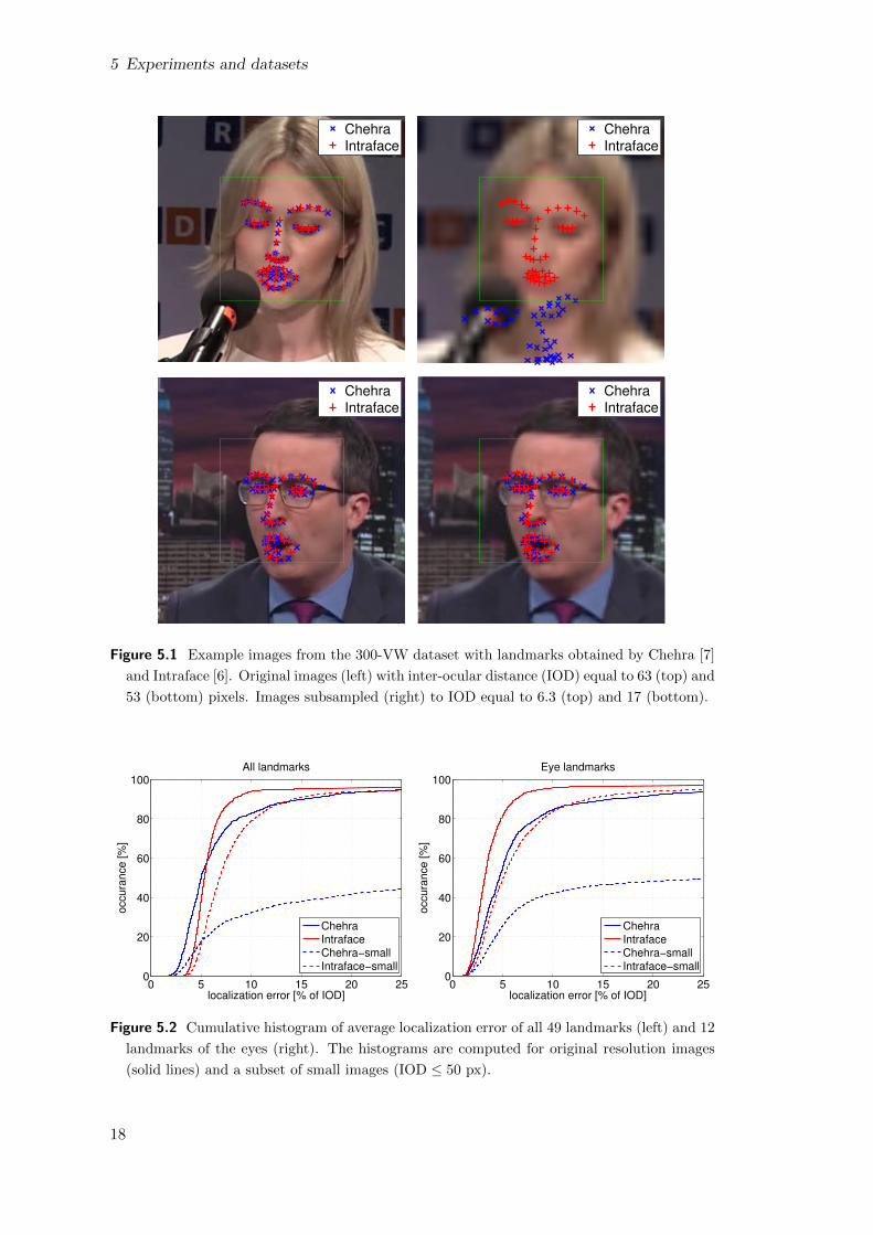
Figure 5.1 Example images from the 300-VW dataset with landmarks obtained by Chehra [7]

and Intraface [6]. Original images (left) with inter-ocular distance (IOD) equal to 63 (top) and

53 (bottom) pixels. Images subsampled (right) to IOD equal to 6.3 (top) and 17 (bottom).

0 5 10 15 20 250

20

40

60

80

100

localization error [% of IOD]

occu

ran

ce

[%

]

All landmarks

Chehra

Intraface

Chehra−small

Intraface−small

0 5 10 15 20 250

20

40

60

80

100

localization error [% of IOD]

occu

ran

ce

[%

]

Eye landmarks

ChehraIntrafaceChehra−smallIntraface−small

Figure 5.2 Cumulative histogram of average localization error of all 49 landmarks (left) and 12

landmarks of the eyes (right). The histograms are computed for original resolution images

(solid lines) and a subset of small images (IOD ≤ 50 px).

18

5.1 Accuracy of landmark detectors

0 20 40 60 80 1000

10

20

30

40

50

IOD [px]

mean e

rror

[% o

f IO

D]

All landmarks

ChehraIntraface

0 20 40 60 80 1000

10

20

30

40

50

IOD [px]

mean e

rror

[% o

f IO

D]

Eye landmarks

ChehraIntraface

Figure 5.3 Landmark localization accuracy as a function of the face image resolution computed

for all landmarks and eye landmarks only.

First, a standard cumulative histogram of the average relative landmark localization

error ε was calculated, see Fig. 5.2, for a complete set of 49 landmarks and also for

a subset of 12 landmarks of the eyes only, since these landmarks are used in the proposed

eye blink detector. The results are calculated for all the original images that have

average IOD around 80 px, and also for all “small” face images (including subsampled

ones) having IOD ≤ 50 px. For all landmarks, Chehra has more occurrences of very

small errors (up to 5 percent of the IOD), but Intraface is more robust having more

occurrences of errors below 10 percent of the IOD. For eye landmarks only, the Intraface

is always more precise than Chehra. As already mentioned, the Intraface is much more

robust to small images than Chehra. This behaviour is further observed in the following

experiment.

Taking a set of all images, we measured a mean localization error µ as a function of

a face image resolution determined by the IOD. More precisely,

µ =1

|S|∑j∈S

εj , (5.2)

i.e. average error over set of face images S having the IOD in a given range. Results

are shown in Fig. 5.3. Plots have errorbars of standard deviation. It is seen that

Chehra fails quickly for images with IOD < 20 px. For larger faces, the mean error is

comparable, although slightly better for Intraface for the eye landmarks.

The last test is directly related to the eye blink detector. We measured accuracy of

EAR as a function of the IOD. Mean EAR error is defined as a mean absolute difference

between the true and the estimated EAR. The plots in Fig. 5.4 are computed for two

subsets: closed/closing (average true ratio 0.05 ± 0.05) and open eyes (average true

ratio 0.4 ± 0.1). The error is higher for closed eyes. The reason is probably that both

detectors are more likely to output open eyes in case of a failure. It is seen that eye

aspect ratio error for IOD < 20 px causes a major confusion between open/closed eye

19


Figure 5.4 Accuracy of the EAR as a function of the face image resolution. Left: for images

with small true ratio (mostly closing/closed eyes), and right: images with higher ratio (open

eyes).

states for Chehra, nevertheless for larger faces the ratio is estimated precisely enough

to ensure a reliable eye blink detection.

5.2 Eye blink detector evaluation

The substantial experiment of the thesis evaluates the proposed blink detectors. Firstly

the available eye blink datasets are presented in 5.2.1. Then the error rates of the eye

blink detectors are detailed and finally experiments on robustness against face resolution

and frame rate are carried out.

As a result of the study measuring the accuracy of landmark detectors in Sec. 5.1,

we decided to use only Intraface [6] landmarks for computation of EAR in Eq. (4.1) in

further experiments due to its excellent performance.

The proposed SVM and HMM based detectors are compared, together with a baseline

method of thresholding of EAR values. The results are reported in Subsec. 5.2.2 and

Subsec. 5.2.3.

There is no standard unified method for measuring accuracy of the eye blink detectors

so the comparison with other methods [3, 23, 1] is only illustrative. We evaluate it

following Fogelton and Benesova [35].

We use an intersection over union overlap

IOU =intersection

union(5.3)

to measure an overlap between the ground-truth and detected blink intervals, see

Fig. 5.5. Pairs of the ground-truth and detected blinks having an overlap over 20

percent are found. These pairs are sorted by its IOU overlap. Then we take the pairs

in decreasing order of IOU and iteratively match the unmatched pairs of blinks with

the highest score of IOU. Pairs where at least one blink is already matched are not

considered anymore. Finally, a number of matched pairs is a number of true positives.

20


Figure 5.5 Intersection over union overlap of ground-truth blink with detected blink.

Unmatched ground-truth blinks are false negatives and unmatched detected blinks are

false positives. So each ground-truth as well as each detected blink is counted only

once.

5.2.1 Datasets for blink detection

We evaluate on three standard datasets with ground-truth annotations of blinks. The an-

notations were normalized to have each blink annotated with its starting and ending

frame.

ZJU

The ZJU [5] dataset is consisting of 80 short videos of 20 subjects. Each subject has

4 videos: 2 with and 2 without glasses, 3 videos are frontal and 1 is an upward view.

The 30fps videos are of size 320 × 240 px. An average video length is 136 frames and

contains about 3.6 blinks in average. An average IOD is 57.4 pixels. In this database,

subjects do not perform any noticeable facial expressions. They look straight into the

camera at close distance, almost do not move, do not either smile nor speak. A ground-

truth blink is defined by its beginning frame, peak frame and ending frame. Examples

of video frames are shown in Fig. 5.6.

Eyeblink8

The dataset Eyeblink8 [3] is more challenging. It consists of 8 long videos of 4 subjects

that are smiling, rotating head naturally, covering face with hands, yawning, drinking

and looking down probably on a keyboard. These videos have length from 5k to 11k

frames, also 30fps, with a resolution 640 × 480 pixels and an average IOD 62.9 pixels.

They contain about 50 blinks on average per video. Each frame belonging to a blink

is annotated by half-open or close state of the eyes. We consider half blinks, which

do not achieve the close state, as full blinks to be consistent with the other datasets.

Examples of video frames are shown in Fig. 5.7.

21


Figure 5.6 Examples of frames of the ZJU dataset [5].

Figure 5.7 Examples of frames of the Eyeblink8 dataset [3].

The Silesian eye blink dataset

The Silesian dataset [50, 34] is recorded in 100 fps in a resolution of 640 × 480 pixels.

It consists of 5 videos of men at close distance in front of the camera. The average

IOD is 146.7 pixels. The scene is very simple. The subjects almost do not move and

they are recorded from frontal position all the sequence. Each video lasts about two

minutes, more accurately they have length from 8k to 16k frames. There are 56 blinks

on average per video sequence.

5.2.2 EAR SVM eye blink detector

The eye blink detector based on SVM is detailed in Sec. 4.1. The SVM classifier

uses a 13-dimensional features for all frame rates. Therefore time windows must be

interpolated to be 13-dimensional for different frame rates than 30 fps. The experiment

with EAR SVM is done in a cross-dataset fashion using all the three blink datasets.

E.g. it means that the SVM classifier is trained on the Eyeblink8 [3] and ZJU [5] and

tested 1 on the Silesian [50, 34] and all three combinations are alternated. The testing

is done using sliding window with a step of a single frame.

Besides testing the proposed EAR SVM method, that is trained to detect the specific

blink pattern, we compare with a simple baseline method, EAR thresholding, which

only thresholds the EAR in Eq. (4.1) values. The precision-recall curves shown in

Fig. 5.9 of the EAR thresholding and EAR SVM classifier were calculated by spanning

a threshold of the EAR and SVM output score respectively. Notice, the precision-recall

curves are not monotonic due to the matching between the ground-truth and detection

blinks involved in the evaluation, see introduction in Sec. 5.2. So it does not hold that

1The EAR SVM detector evaluates only frames in the middle of a blink as positives but we need to

have positive detection during the whole blink because of evaluating using overlap with the ground-

truth. Thus we need to extend the detected blinks by ±100 ms (±3 frames while having 30fps

videos) to obtain a longer pulse of a detected blink.

22


Figure 5.8 An example pointing to how difficult is to set a correct threshold while thresholding

the EAR curve. If the threshold is set to 0.35 the left blink will be detected but in right half

of a plot there would be long false positive. If the threshold is set to 0.2 then the right blink

is detected but the left blink is missed.

with increasing recall it decreases precision and vice versa. For easier comparison the

operational points with the highest F1 score (5.4) were extracted from the precision-

recall curves and published in Tab. 5.1.

F1 = 2precision.recall

precision+ recall(5.4)

It is very difficult to estimate a correct threshold convenient for all the video se-

quences, see example in Fig. 5.8. So the thresholding method makes many mistakes.

The proposed EAR SVM detector outperforms the methods by Drutarovsky and Fo-

gelton [3], Lee et al. [23] and Danisman et al. [1]. The method by Fogelton and Be-

nesova [35] is comparable with ours for Eyeblink8 and Silesian datasets. But we slightly

leg behind the method by Fogelton and Benesova [35] at the ZJU dataset. We have

counted more false negatives. However, we believe that this is mostly caused by the fact

that the videos from ZJU frequently start or end during the blink and a whole blink

time window is needed for EAR SVM classification. The results of the other methods

are depicted with our precision-recall curves in Fig. 5.9.

23


Figure 5.9 Precision-recall curves of the EAR thresholding, EAR SVM and EAR adaptive

HMM classifiers measured on the ZJU (top row), the Eyeblink8 (middle row) and the Silesian

(bottom row) datasets. The operational points with the highest F1 score (5.4) for thresholding

(resp. SVM) method are drawn by green (resp. red) points. Published results of methods

A - Drutarovsky and Fogelton [3], B - Lee et al. [23], C - Danisman et al. [1], D - Fogelton

and Benesova [35] are depicted. Plots in the right column are zoomed to those on the left.

24


5.2.3 EAR adaptive HMM eye blink detector

The EAR adaptive HMM method and its parameters are detailed in Sec. 4.2. The generic

parameters of the HMM are learned using the ground-truth annotation from datasets

ZJU and Eyeblink8. The first state is open eye and the second state is closed eye.

The generic transition matrix is set:

AG =

[0.99 0.01

0.11 0.89

], (5.5)

generic initial probabilities are:

πG =[0.98 0.08

](5.6)

generic means for open and close state are determined as:

µG =[0.3 0.11

](5.7)

and generic standard deviations:

σG =[0.06 0.04

]. (5.8)

The parameters for adaptation of the model are set experimentally. Older models

than the learning time:

L = 40s (5.9)

are forgotten. The subsequence size of the time window used for learning new model

parameters is:

S = 1s, (5.10)

the interval of recomputation of a new model is:

I = 1s, (5.11)

and the threshold:

D = 0.15, (5.12)

which is described in Subsec. 4.2.3. An interpretation of the parameters is illustrated

in Fig. 4.4.

The results of eye blink detection of EAR adaptive HMM method are depicted in

Fig. 5.9 together with the results of EAR SVM and EAR thresholding. We can see

that the EAR adaptive HMM has better results in a comparison with the baseline

method of EAR thresholding on all the three datasets. But apart from the ZJU dataset

the unsupervised EAR adaptive HMM classifier is a little bit worse compared with

the supervised EAR SVM method. Some of the errors of the EAR adaptive HMM

method are caused by slow adaptation of the model. If a person-specific model vary

25


Figure 5.10 An example of a weak blink. Only the EAR adaptive HMM method correctly

detects the blink.

ZJU Eyeblink8 Silesian

thr. SVM HMM thr. SVM HMM thr. SVM HMM

precision 89.2 97.7 98.8 77.9 94.3 92.1 74.2 93.0 91.4

recall 98.5 92.9 92.2 77.9 96.2 85.5 94.0 98.6 82.9

threshold 0.27 1.2 - 0.08 0.2 - 0.15 0.4 -

Table 5.1 The operational points having the highest F1 score (5.4) from all points in precision-

recall curves of thresholding and EAR SVM method. The result of EAR adaptive HMM for

three standard datasets.

26


a lot from the generic one or a person squints its eyes by smiling for example, it lasts

some time to adapt the model parameters. Another part of the error of the HMM

based method rises on the transition between open and half-open eyes. When a subject

squints his/her eyes, but does not close the eyes fully, the system firstly detects the

half-open eyes as closed and then it adapts to consider them as open. So the eyes are

detected as closed only at the beginning of eyes squeezing. The symmetric situation

happens at the end of eye squeezing. Nevertheless, there are multiple situations where

EAR adaptive HMM method is better than EAR SVM, for example when a blink is

not very dominant. In Fig. 5.10 the blink impulse is very weak and all the methods fail

except the EAR adaptive HMM.

An important advantage of the eye blink detector using hidden Markov model is that

it can distinguish between open and close states even out of blinking. Besides computing

a frequency of blinking it is thus capable to determine a duration of a particular eye

closure and so it can measure the total time of eyes being closed. This can be very

useful to detect a subject’s drowsiness which is reflected in the eye blink duration and

frequency.

5.2.4 Computation of blink statistics

The main blink properties are blink frequency, duration, amplitude and a speed of eyelid

movement while closing or opening the eye. We measure blink frequency, duration and

amplitude at this experiment.

Blink frequency

Firstly a number of detected blinks ND is compared with a number of ground-truth

blinks NGT . Then the frequencies of detected FD and ground-truth FGT blinks are

compared. We use a number of blinks per minute unit. The statistics are listed in

Tab. 5.2 for each video of Eyeblink8 and Silesian datasets. Because the ZJU dataset

contains 80 videos, we do not show results of each video separately but only for the

whole dataset. The average blink frequency is 17 blinks per min, during conversation

it increase to 26 and it decreases to 5 blinks per minute while reading according to

the literature [51]. Based on these assumptions we can suspect that people are more

concentrated in Eyeblink8. There is a little above average blink frequency at Silesian

although they are not talking. But at ZJU the blink frequency about 45 blinks per

minute is really abnormal. We believe that the subjects are not blinking spontaneously

and they were informed that they were recorded for the purpose of a blink study.

Blink duration

The important property of blinking besides frequency is blink duration. Every person

has a little bit different length of an average blink and it can also reflect a person’s

drowsiness and mood. We are unable to measure a blink duration using EAR SVM

27


Eyeblink8

Video name NGT ND ND FGT FD FD Err SVM Err HMM

SVM HMM [#b/min] SVM HMM [%] [%]

Eyeblink8 1 30 32 24 4.8 5.2 3.9 +6.6 -20.0

Eyeblink8 2 88 88 73 14.4 14.4 11.9 0.0 -17.1

Eyeblink8 3 61 57 66 11.9 11.6 12.9 -6.5 +8.2

Eyeblink8 4 31 31 32 10.6 10.6 11.0 0.0 +3.2

Eyeblink8 5 73 73 66 14.7 14.7 13.3 0.0 -9.6

Eyeblink8 6 43 42 36 16.4 15.8 13.5 -2.3 -16.3

Eyeblink8 7 29 33 34 4.9 5.6 5.8 +13.8 +17.3

Eyeblink8 8 39 42 35 14.3 15.4 12.9 +7.7 -10.3

All videos 394 398 366 10.8 10.9 10.0 +1.0 -7.1

Silesian

Video name NGT ND ND FGT FD FD Err SVM Err HMM


Silesian 1 88 90 69 45.9 47.0 36.0 +2.3 -21.6

Silesian 2 31 38 35 11.6 14.2 13.1 +22.6 +12.9

Silesian 3 54 57 49 31.7 33.5 28.8 +5.6 -9.3

Silesian 4 77 80 70 35.1 36.4 31.9 +3.9 -9.1

Silesian 5 31 33 32 22.9 24.4 23.6 +6.5 +3.2

All videos 281 298 255 28.6 30.3 25.9 +5.0 -9.2

ZJU

NGT ND ND FGT FD FD Err SVM Err HMM


All videos 269 262 251 44.5 43.4 41.5 -2.6 -9.3

Table 5.2 Blink frequencies of Eyeblink8, Silesian and ZJU datasets. NGT is a number of

ground-truth blinks, ND is a number of detected blinks either by EAR SVM method or by

method using EAR adaptive HMM. FGT (resp. FD) is an average number of ground-truth

blinks (resp. detected blinks either by SVM or HMM) per one minute. The last two columns

show error in percent.

28


Eyeblink8

Video name µGT µD Err µ σGT σD Err σ Closed eyes [%]

Eyeblink8 1 371 274 -98 273 156 -117 6.3

Eyeblink8 2 437 349 -87 167 120 -47 9.7

Eyeblink8 3 307 271 -36 95 118 +23 7.0

Eyeblink8 4 352 273 -79 146 117 -30 5.5

Eyeblink8 5 272 243 -29 78 122 +44 11.2

Eyeblink8 6 262 297 +35 103 164 +62 17.4

Eyeblink8 7 300 250 -50 64 109 +46 8.2

Eyeblink8 8 375 254 -121 182 109 -73 12.3

All videos 339 281 -58 157 130 -27 9.1

Silesian

Video name µGT µD Err µ σGT σD Err σ Closed eyes [%]

Silesian 1 365 297 -69 101 167 +66 27.9

Silesian 2 294 265 -28 63 164 +101 10.7

Silesian 3 378 227 -151 183 152 -31 22.0

Silesian 4 345 245 -100 74 114 +40 22.5

Silesian 5 368 209 -159 109 93 -15 9.4

All videos 354 254 -101 115 145 +30 18.5

ZJU

µGT µD Err µ σGT σD Err σ Closed eyes [%]

All videos 262 187 -75 105 94 -11 13.2

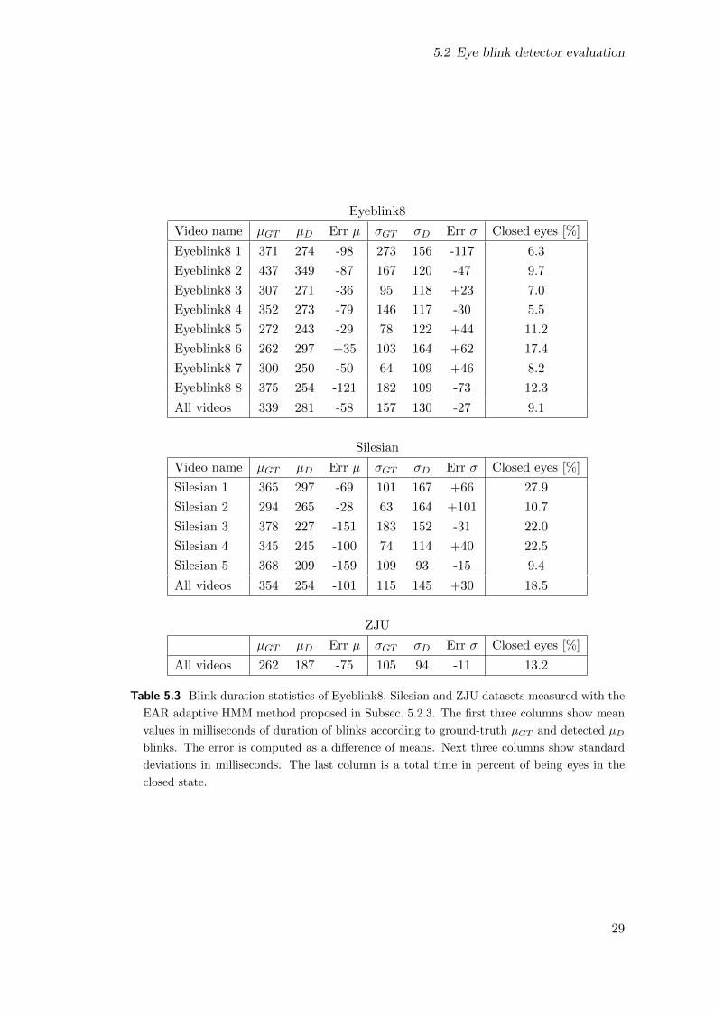
Table 5.3 Blink duration statistics of Eyeblink8, Silesian and ZJU datasets measured with the

EAR adaptive HMM method proposed in Subsec. 5.2.3. The first three columns show mean

values in milliseconds of duration of blinks according to ground-truth µGT and detected µD

blinks. The error is computed as a difference of means. Next three columns show standard

deviations in milliseconds. The last column is a total time in percent of being eyes in the

closed state.

29


min ymax max ymax µ ymax σ ymax

0.11 0.42 0.29 0.06

Table 5.4 Minimal, maximal, mean and standard deviation from average ymax from all videos.

Figure 5.11 The blink amplitude ymax.

classifier because it detects only peak of an eye blink. Therefore we must use the EAR

adaptive HMM method proposed in Subsec. 5.2.3. This method defines blinks as eye

closure longer than 60 ms and shorter than 700 ms. The following experiment measures

eye blink duration and estimates a total time of eyes being in a closed state.

From results depicted in Tab. 5.3 we can see that the average blink length is about

250 milliseconds. The detected mean values and standard deviations of blink duration

are compared with the ground-truth. However, we note that the annotation of blinks

is of a limited precision. It is very subjective and tedious to delineate the start and

end of a single blink precisely and including at Silesian dataset which is recorded at a

higher frame rate of 100 fps.

Blink amplitude

Another interesting blink statistics is a blink amplitude ymax which describes the degree

of openness. It differs between people and it also depends on head pose. The blink

amplitude is the mean difference between EAR at open state and at closed state, see

Fig. 5.11. The purpose of this experiment is to show that blink amplitudes vary a lot.

For each video we measured average maximal amplitude ymax while blinking. Then

we have computed minimal, maximal, mean and standard deviation from ymax from all

videos in Tab. 5.4. The histogram of ymax values is shown in Fig. 5.12.

Figure 5.12 The histogram of average amplitude ymax calculated for each video.

30


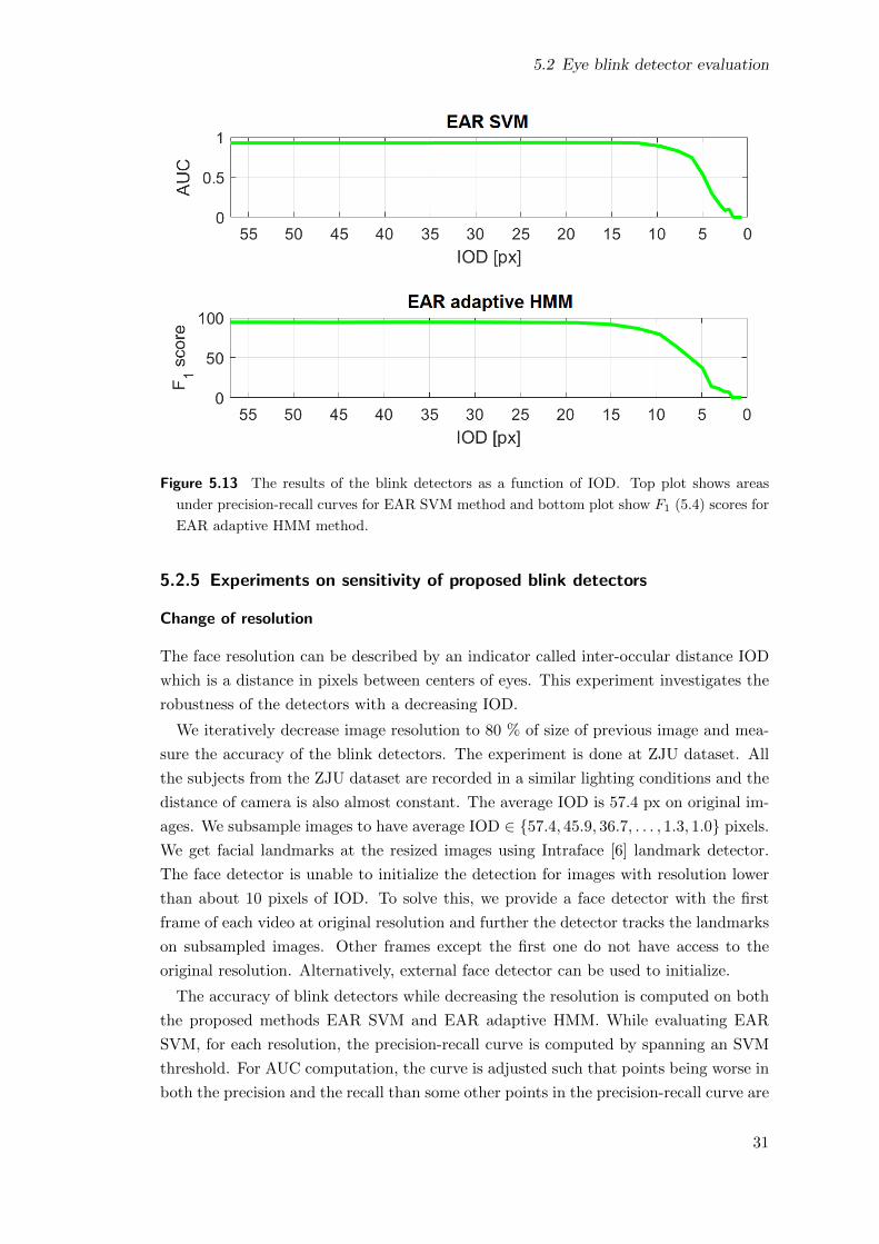
Figure 5.13 The results of the blink detectors as a function of IOD. Top plot shows areas

under precision-recall curves for EAR SVM method and bottom plot show F1 (5.4) scores for

EAR adaptive HMM method.

5.2.5 Experiments on sensitivity of proposed blink detectors

Change of resolution

The face resolution can be described by an indicator called inter-occular distance IOD

which is a distance in pixels between centers of eyes. This experiment investigates the

robustness of the detectors with a decreasing IOD.

We iteratively decrease image resolution to 80 % of size of previous image and mea-

sure the accuracy of the blink detectors. The experiment is done at ZJU dataset. All

the subjects from the ZJU dataset are recorded in a similar lighting conditions and the

distance of camera is also almost constant. The average IOD is 57.4 px on original im-

ages. We subsample images to have average IOD ∈ {57.4, 45.9, 36.7, . . . , 1.3, 1.0} pixels.

We get facial landmarks at the resized images using Intraface [6] landmark detector.

The face detector is unable to initialize the detection for images with resolution lower

than about 10 pixels of IOD. To solve this, we provide a face detector with the first

frame of each video at original resolution and further the detector tracks the landmarks

on subsampled images. Other frames except the first one do not have access to the

original resolution. Alternatively, external face detector can be used to initialize.

The accuracy of blink detectors while decreasing the resolution is computed on both

the proposed methods EAR SVM and EAR adaptive HMM. While evaluating EAR

SVM, for each resolution, the precision-recall curve is computed by spanning an SVM

threshold. For AUC computation, the curve is adjusted such that points being worse in

both the precision and the recall than some other points in the precision-recall curve are

31


Figure 5.14 Example of detected blinks at small resolution of 9 px of IOD. The plots of

the eye aspect ratio EAR in Eq. (4.1), results of the EAR thresholding (threshold set to

0.2), the blinks detected by EAR SVM, the blinks detected by EAR adaptive HMM and the

ground-truth labels over the video sequence. Input image with detected landmarks (depicted

frame is marked by a red line). All blinks were detected correctly by all the proposed methods.

32


Figure 5.15 Example of detected blinks at extremely small resolution of IOD = 2.5 px.

The plots of the eye aspect ratio EAR in Eq. (4.1), results of the EAR thresholding (threshold

set to 0.2), the blinks detected by EAR SVM, the blinks detected by EAR adaptive HMM

and the ground-truth labels over the video sequence. Input image with detected landmarks

(depicted frame is marked by a red line). Most of the blinks were detected correctly by

the proposed methods.

33


filtered out. The AUC is depicted in a top plot of Fig. 5.13. There is no precision-recall

curve while evaluating EAR adaptive HMM because we obtain only one precision-recall

point for each resolution. The F1 score (5.4) is computed and plotted in a bottom plot

of Fig. 5.13.

Until the IOD = 15 px both the detectors are excellent. Then the EAR adaptive

HMM method starts to slowly decrease its performance. The EAR SVM holds a very

good result up to IOD = 10 px which is really surprising. See example in Fig. 5.14

where all blinks were correctly detected even at IOD = 10 px.

Astonishingly, there are videos at which blink detectors partly work as low as IOD

is 2.5 px. Interpret an image/video in such a low resolution is difficult for human.

An example is shown in Fig. 5.15. All the proposed methods correctly determined

4 blinks from 5. They have at most two mistake, but the last blink should not be

computed, because it is not the full blink. The landmarks are not obviously accurate

at all but they still reflect a movement of eyelids and thus they also reflect a change of

EAR.

The facial landmark detectors are very precise even at low resolution. Further effort

to improve an estimation of a level of eye openness directly from image may be very

difficult. Ability of the blink detector to work with low resolution images allows possible

applications where a consumer webcamera or a surveillance camera are used. Blinking

of a subject is monitored in a surprisingly large distance for even a group of people.

Change of frame rate

The dependence of detector accuracy on frame rate is tested at this experiment. The

videos are transformed to different frame rates by omitting some frames. This may be

a little bit different from decreasing frame rate due to long camera exposure which may

produce blurred images. So the new frame rates are set to be divisors of original frame

rate. The 30fps videos are transformed to have 30, 15, 10, 6, 5, 3, 2 and 1 frame per

second and 100fps videos have new frame rates equal to 100, 50, 25, 20, 10, 5, 4, 2 and

1. The experiment is done on the ZJU, Eyeblink8 and Silesian datasets. The results

for higher frame rate than 30 fps at Silesian dataset are not shown because they almost

do not change.

Fig. 5.16 show results of EAR SVM blink detector in dependence of frame rate.

The EAR SVM method does not produce one precision-recall point so the area under

the precision-recall curve is computed for each frame rate. The AUC is computed in the

same way as while evaluating change of IOD experiment. The results of EAR adaptive

HMM method are shown in Fig. 5.17. The F1 score (5.4) is evaluated for each frame

rate.

We can see that both the curves in Fig. 5.16 and Fig. 5.17 showing the accuracy of

the detectors are very similar. The accuracy is almost unchanged until 10 fps. Then

it begins slightly worsen and from 5 fps it fails quickly. So the conclusion is that both

EAR SVM and EAR adaptive HMM methods work very well until frame rate of 10 fps.

34


Figure 5.16 The area under precision-recall curve computed for iteratively decreasing frame

rate using EAR SVM method.

Figure 5.17 The F1 score computed for iteratively decreasing frame rate using EAR adaptive

HMM method.

35

6 Eye blink detector application

I explore drowsiness during the day as an application of the eye blink detection.

I recorded short videos of myself working on a laptop. My drowsiness is estimated

from blink characteristics such as frequency and average duration.

I recorded 1-minute long videos during the day. I used a web camera on my laptop

and a web camera Logitech C920 that both recorded in 640 × 480 px resolution. These

cameras, especially the built-in web camera, are of a consumer quality. There is a lot of

noise and very poor contrast and sharpness, particularly in a weak night illumination.

The frame rate depends on an illumination and on a computer workload but it varies

from 8 to 30 fps. The recording was triggered randomly in about 15 minutes inter-

vals. I was not aware exactly while I was recorded. I collected the videos for 10 days

while I was intensively working on my diploma thesis. The video sequences are quite

challenging because of varied head poses, face occlusions and poor quality of images.

I often look on a keyboard and sometimes I look on a screen, for a very short time

on a keyboard and again on a screen which may have been misinterpreted as blinking.

Surprisingly, I found out that I frequently subconsciously put my hands on face, most

often on my mouth or my nose. These occlusions may be distracting for the landmark

detector. Examples of video frames with various illumination, occlusions and noise are

shown in Fig. 6.1 .

All the videos having detected face less then 80% of the time were discarded. It hap-

pened mostly when I was out of field of view of the camera and I forgot to stop recording

or when I wrote something on a table and I had bent down my head for most of time

of the 1-minute recording. The Intraface [6] system is used to detect facial landmarks.

Both the eye blink detection method proposed in Sec. 4.1 and Sec. 4.2 are applied.

A day is divided into 24 bins where 1 bin represents 1 hour. The videos were recorded

from 7 a.m. to 1 a.m. of the following day. There were recorded from 4 to 35 videos

for each hour, averagely 15 videos per hour, in total 355 1-minute videos.

A commonly used drowsiness identifier PERCLOS1 [36] is not suitable for monitoring

fatigue of a subject working on a laptop because of frequent looking down on a keyboard.

This could be misinterpreted from a view of the camera as closed eyes. So we use

an average blink frequency and duration as main drowsiness indicators for all the videos.

The results are assigned to the bins according to a time of the recording. The duration

is computed using EAR adaptive HMM method, because EAR SVM method cannot

correctly determine a blink length. The frequency is computed by both the EAR SVM

and EAR adaptive HMM and averaged.

1PERCLOS determines a time having closed eyes at least 80%

36

Figure 6.1 Various examples of video frames used for eye blink drowsiness application.

Let us define a relative drowsiness index κ as a function of average blink frequency

F (blinks per minute) and duration Z (in ms) computed for each hour during a day.

The frequency and the duration are normalized to have zero mean and standard devi-

ation equal to one. The formula for calculation κ is chosen so that the frequency and

duration have the same weight:

κ = Fnorm + Znorm. (6.1)

The drowsiness index κ of the recorded videos is shown in Fig. 6.2. I can fairly con-

firm the measured drowsiness index curve which corresponds to my subjective feelings.

I usually have slow mornings and it starts to get better at about 10 a.m.. After having

lunch, the afternoon is almost balanced but I can honestly say that at about 9 p.m.

I work best. This corresponds to the measured drowsiness index which starts to get

lower at 8 p.m. and from 11 p.m. it grows quickly.

The means and standard deviations of blink frequency and blink duration computed

at collected videos are depicted in Fig. 6.3. The standard deviations are quite big which

may be caused by the fact that the activities are changed within one hour, e.g. blink

frequency while reading differs from blink frequency while thinking or writing.

We note that the blink measurements may not be completely accurate because some-

times the videos are only about 10 fps due to long camera exposure while having poor

lighting conditions. Nevertheless, this simple experiment confirms that the drowsiness

may be monitored by simple blink characteristics such as blink duration and blink

frequency.

37

6 Eye blink detector application

Figure 6.2 Blink characteristics of a subject working on her diploma thesis measured each

hour during a day. A result is averaged from 10 days. Normalized blink frequency (green)

per minute is computed and averaged from EAR SVM and EAR adaptive HMM outputs.

Normalized blink duration (red) is computed using EAR adaptive HMM method. Drowsiness

index (blue) as a function of normalized blink frequency and normalized blink duration.

Figure 6.3 Blink frequency and blink duration over the day. The plots have errorbars of stan-

dard deviation.

38

7 Implementation details

A processing time is computed using Eyeblink8 dataset which is recorded in a resolution

of 640 × 480 px and have IOD about 62.9 px. An average time for processing one frame

using EAR SVM is 19.2 ms and using EAR adaptive HMM it is 18.7 ms. These times

already include a processing time taken for finding facial landmarks. Thus the proposed

algorithms run in about 50-60 fps while using ordinary laptop (64-bit Windows 8, Intel

Core [email protected] GHz, 8GB RAM).

A real-time blink detector demo has been prepared. It runs in Matlab and uses OpenCV

to capture images from a laptop webcamera. A beep sounds when a subject being in

a field of view of a camera blinks.

The main part of the work is programmed in Matlab R2015b. Some parts, especially

collecting of videos of myself for the application, are written in C++. The OpenCV [52]

library is used for capturing and processing images. The recording of videos is done

using standard built-in laptop webcamera and Logitech C920 webcamera. The text is

written in LATEX in online environment Overleaf [53].

39

8 Conclusion

Real-time eye blink detection algorithms were introduced. We quantitatively demon-

strated that regression-based facial landmark detectors are precise enough to reliably

estimate a level of eye openness. While they are robust to low image quality (low im-

age resolution in a large extent) and in-the-wild phenomena as bad illumination, facial

expressions, etc.

Two methods for blink detection were proposed. Both methods use a single scalar

quantity, eye aspect ratio, estimated from landmark locations detected for each frame

of a video sequence. The eye blink detection based on an SVM classifier, that takes

a temporal window of the EARs, is presented in the first method. The second approach

uses a hidden Markov model to decide between the open and closed eye states. A simple

state machine detecting blinks according to eye closure lengths is then deployed. Finally,

the HMM based method is equipped with an adaptation mechanism that adjusts model

parameters to fit well to a subject being observed over time.

The proposed methods were thoroughly experimentally tested and qualitatively eval-

uated on three standard datasets. A comparison with a baseline EAR thresholding

as well as with several state-of-the-art algorithms proved competitive results. The

SVM based method outperforms method using HMM except for the ZJU dataset where

the methods have almost the same result. On the other hand, the HMM method can

be used even when recognizing eye closures longer than average eye blink which cannot

be done by SVM approach. Another advantage of the HMM based method is that it is

unsupervised unlike the SVM method which needs annotated training data.

The proposed algorithms run in real-time (50 fps), since the additional computational

costs for the eye blink detection are negligible besides the real-time landmark detectors.

We see a limitation in the eye openness estimate. While EAR is estimated from a 2D

image, it is fairly insensitive to a head orientation, but it may lose discriminability

for out of face rotations. A solution might be to define the EAR in 3D. There are

landmark detectors that estimate a 3D pose (position and orientation) of a 3D model

of landmarks [8, 7].

40

Bibliography

[1] T. Danisman, I. Bilasco, C. Djeraba, and N. Ihaddadene, “Drowsy driver detection

system using eye blink patterns,” in Machine and Web Intelligence (ICMWI), Oct

2010. 2, 5, 9, 20, 23, 24

[2] M. Divjak and H. Bischof, “Eye blink based fatigue detection for prevention of

computer vision syndrome,” 2009. 2, 7

[3] T. Drutarovsky and A. Fogelton, “Eye blink detection using variance of motion

vectors,” in Computer Vision - ECCV Workshops, 2014. 2, 7, 8, 20, 21, 22, 23, 24

[4] “An adaptive blink detector to initialize and update a view-basedremote eye gaze

tracking system in a natural scenario,” Pattern Recognition Letters, vol. 30, no. 12,

pp. 1144 – 1150, 2009. 2

[5] G. Pan, L. Sun, Z. Wu, and S. Lao, “Eyeblink-based anti-spoofing in face recogni-

tion from a generic webcamera,” in ICCV, 2007. 2, 21, 22

[6] X. Xiong and F. De la Torre, “Supervised descent methods and its applications to

face alignment,” in Proc. CVPR, 2013. 2, 17, 18, 20, 31, 36

[7] A. Asthana, S. Zafeoriou, S. Cheng, and M. Pantic, “Incremental face alignment

in the wild,” in Conference on Computer Vision and Pattern Recognition, 2014. 2,

12, 17, 18, 40

[8] J. Cech, V. Franc, M. Uricar, and J. Matas, “Multi-view facial landmark detection

by using a 3d shape model,” Image and Vision Computing, vol. 47, pp. 60 – 70,

2016. 2, 40

[9] D. Yolton, R. Yolton, R. Lopez, B. Bogner, R. Stevens, and D. Rao, “The effects

of gender and birth control pill use on spontaneous blink rates.” Pacific University

College of Optometry, Forest Grove, OR 97116, Nov 1994. 4

[10] J. J. Tecce, “Psychology, physiological and experimental,” 1992. 4

[11] M. Pal, A. Banerjee, S. Datta, A. Konar, D. N. Tibarewala, and R. Janarthanan,

“Electrooculography based blink detection to prevent computer vision syndrome,”

in Electronics, Computing and Communication Technologies (IEEE CONECCT),

2014 IEEE International Conference on, pp. 1–6, Jan 2014. 5

41

Bibliography

[12] Y. Kim, “Detection of eye blinking using doppler sensor with principal component

analysis,” IEEE Antennas and Wireless Propagation Letters, vol. 14, pp. 123–126,

2015. 5

[13] C. Tamba, S. Tomii, and T. Ohtsuki, “Blink detection using doppler sensor,” in

2014 IEEE 25th Annual International Symposium on Personal, Indoor, and Mobile

Radio Communication (PIMRC), pp. 2119–2124, Sept 2014. 5

[14] Medicton group, “The system I4Control.” http://www.i4tracking.cz/. 5

[15] A. Haro, M. Flickner, and I. Essa, “Detecting and tracking eyes by using their phys-

iological properties, dynamics, and appearance,” in Computer Vision and Pattern

Recognition, 2000. Proceedings. IEEE Conference on, vol. 1, pp. 163–168 vol.1,

2000. 5

[16] L. M. Bergasa, J. Nuevo, M. A. Sotelo, R. Barea, and M. E. Lopez, “Real-time

system for monitoring driver vigilance,” IEEE Transactions on Intelligent Trans-

portation Systems, vol. 7, pp. 63–77, March 2006. 5

[17] I. Garca, S. Bronte, L. M. Bergasa, J. Almazn, and J. Yebes, “Vision-based drowsi-

ness detector for real driving conditions,” in Intelligent Vehicles Symposium (IV),

2012 IEEE, pp. 618–623, June 2012. 5

[18] A. Panning, A. Al-Hamadi, and B. Michaelis, “A color based approach for eye

blink detection in image sequences,” in Signal and Image Processing Applications

(ICSIPA), 2011 IEEE International Conference on, pp. 40–45, Nov 2011. 5

[19] F. Yang, X. Yu, J. Huang, P. Yang, and D. Metaxas, “Robust eyelid tracking for

fatigue detection,” in ICIP, 2012. 5, 9

[20] F. M. Sukno, S.-K. Pavani, C. Butakoff, and A. F. Frangi, “Automatic assessment

of eye blinking patterns through statistical shape models,” in ICVS, 2009. 5, 7, 8

[21] H. Dinh, E. Jovanov, and R. Adhami, “Eye blink detection using intensity vertical

projection,” 2012. 5, 6

[22] Y. Xu, Y. Jiang, and Y. Sun, “Blink detection using 3d cross model,” in Compu-

tational Intelligence and Design (ISCID), 2012 Fifth International Symposium on,

vol. 2, pp. 115–118, Oct 2012. 5

[23] W. H. Lee, E. C. Lee, and K. E. Park, “Blink detection robust to various facial

poses,” Journal of Neuroscience Methods, Nov. 2010. 5, 6, 20, 23, 24

[24] M. Awais, N. Badruddin, and M. Drieberg, “Automated eye blink detection and

tracking using template matching,” in Research and Development (SCOReD), 2013

IEEE Student Conference on, pp. 79–83, Dec 2013. 5

42

http://www.i4tracking.cz/

Bibliography

[25] A. Krolak and P. Strumi l lo, “Eye-blink detection system for human–computer

interaction,” Universal Access in the Information Society, vol. 11, no. 4, pp. 409–

419, 2012. 5, 6

[26] M. Chau and M. Betke, “Real time eye tracking and blink detection with usb

cameras,” tech. rep., 2005. 5, 6

[27] A. Udayashankar, A. R. Kowshik, S. Chandramouli, and H. S. Prashanth, “Assis-

tance for the paralyzed using eye blink detection,” in Digital Home (ICDH), 2012

Fourth International Conference on, pp. 104–108, Nov 2012. 5

[28] M. Lalonde, D. Byrns, L. Gagnon, N. Teasdale, and D. Laurendeau, “Real-time

eye blink detection with gpu-based sift tracking,” in Computer and Robot Vision,

2007. CRV ’07. Fourth Canadian Conference on, pp. 481–487, May 2007. 7

[29] P. S. Parmar and N. Chitaliya, “Detect eye blink using motion analysis method,”

2013. 7

[30] Y. Kurylyak, F. Lamonaca, and G. Mirabelli, “Detection of the eye blinks for hu-

man’s fatigue monitoring,” in Medical Measurements and Applications Proceedings

(MeMeA), 2012 IEEE International Symposium on, pp. 1–4, May 2012. 7

[31] M. Divjak and H. Bischof, “Real-time video-based eye blink analysis for detection

of low blink-rate during computer use,” 2008. 7

[32] J. Mohanakrishnan, S. Nakashima, and J. Odagiri, “A novel blink detection system

for user monitoring,” in User-Centered Computer Vision (UCCV), 2013 1st IEEE

Workshop on, pp. 37–42, Jan 2013. 7

[33] L. Pauly and D. Sankar, “A novel method for eye tracking and blink detection

in video frames,” in 2015 IEEE International Conference on Computer Graphics,

Vision and Information Security (CGVIS), pp. 252–257, Nov 2015. 7

[34] K. Radlak and B. Smolka, “A novel approach to the eye movement analysis using

a high speed camera,” in Advances in Computational Tools for Engineering Appli-

cations (ACTEA), 2012 2nd International Conference on, pp. 145–150, Dec 2012.

7, 22

[35] A. Fogelton and W. Benesova, “Eye blink detection based on motion vectors anal-

ysis,” 2016. 7, 20, 23, 24

[36] W. W. Wierwille, S. S. Wreggit, C. L. Kirn, L. A. Ellsworth, and R. J. Fairbanks,

“Research on vehicle-based driver status/performance monitoring; development,

validation, and refinement of algorithms for detection of driver drowsiness,” tech.

rep., Virginia Polytechnic Institute and State University, Blacksburg, National

Highway Traffic Safety Administration, 12 1994. 8, 9, 36

43

Bibliography

[37] L. Wang, X. Ding, C. Fang, C. Liu, and K. Wang, “Eye blink detection based on

eye contour extraction,” in Conference: Image Processing: Algorithms and Systems

VII, 2009. 8, 9

[38] L. Pauly and D. Sankar, “Detection of drowsiness based on hog features and svm

classifiers,” in 2015 IEEE International Conference on Research in Computational

Intelligence and Communication Networks (ICRCICN), pp. 181–186, Nov 2015. 9

[39] I. Saeed, A. Wang, R. Senaratne, and S. Halgamuge, “Using the active appear-

ance model to detect driver fatigue,” in 2007 Third International Conference on

Information and Automation for Sustainability, pp. 124–128, Dec 2007. 9

[40] G. L. R. Clavijo, J. O. Patio, and D. M. Len, “Detection of visual fatigue by analyz-

ing the blink rate,” in Signal Processing, Images and Computer Vision (STSIVA),

2015 20th Symposium on, pp. 1–5, Sept 2015. 9

[41] Y. Kurylyak, F. Lamonaca, G. Mirabelli, O. Boumbarov, and S. Panev, “The in-

frared camera-based system to evaluate the human sleepiness,” in Medical Measure-

ments and Applications Proceedings (MeMeA), 2011 IEEE International Workshop

on, pp. 253–256, May 2011. 9

[42] A. Rahman, M. Sirshar, and A. Khan, “Real time drowsiness detection using eye

blink monitoring,” in 2015 National Software Engineering Conference (NSEC),

pp. 1–7, Dec 2015. 9

[43] Q. Ji, Z. Zhu, and P. Lan, “Real-time nonintrusive monitoring and prediction of

driver fatigue,” IEEE Transactions on Vehicular Technology, vol. 53, pp. 1052–

1068, July 2004. 9, 10

[44] L. R. Rabiner, First-Hand:The Hidden Markov Model. 2013. 13

[45] J. Li, “Hidden markov model.” http://sites.stat.psu.edu/~jiali/course/

stat597e/notes2/hmm.pdf. 13

[46] J. A. Bilmes, “A gentle tutorial of the em algorithm and its application to param-

eter estimation for gaussian mixture and hidden markov models,” April. 13

[47] A. Viterbi, “Error bounds for convolutional codes and an asymptotically optimum

decoding algorithm,” IEEE Transactions on Information Theory, vol. 13, pp. 260–

269, April 1967. 13, 14

[48] A. P. Dempster, N. M. Laird, and D. B. Rubin, “Maximum Likelihood from In-

complete Data via the EM Algorithm,” Journal of the Royal Statistical Society.

Series B (Methodological), vol. 39, no. 1, pp. 1–38, 1977. 14

[49] S. Zafeiriou, G. Tzimiropoulos, and M. Pantic, “The 300 videos in the wild (300-

VW) facial landmark tracking in-the-wild challenge,” in ICCV Workshop, 2015.

http://ibug.doc.ic.ac.uk/resources/300-VW/. 17

44

http://sites.stat.psu.edu/~jiali/course/stat597e/notes2/hmm.pdf

http://sites.stat.psu.edu/~jiali/course/stat597e/notes2/hmm.pdf

http://ibug.doc.ic.ac.uk/resources/300-VW/

Bibliography

[50] K. Radlak and B. Smolka, “Blink detection based on the weighted gradient descrip-

tor,” in Proceedings of the 8th International Conference on Computer Recognition

Systems CORES 2013, pp. 691–700, Springer International Publishing, 2013. 22

[51] A. R.Bentivoglio, S. Bressman, E. Cassetta, D. Carretta, P. Tonali, and A. Al-

banese, “Analysis of blink rate patterns in normal subjects,” 1997. 27

[52] G. Bradski Dr. Dobb’s Journal of Software Tools. 39

[53] “Overleaf.” http://www.overleaf.com/. Accessed: 2016-05-22. 39

45

http://www.overleaf.com/

Documents

CENTER FOR MACHINE PERCEPTION Eye-Blink Detection Using ... · Title of Diploma Thesis : Eye -Blink Detection Using Facial Landmarks . Guidelines: 1. Propose an eye- blink detection