Embed Size (px)
Citation preview

Central Bedfordshire Councilwww.centralbedfordshire.gov.uk
Central BedfordshireDevelopment StrategyEcosystem Services Appendices
Publication January 2013
Security classification:
Protected


Spatial Evidence Base to improve Regulating Ecosystem Services in Central Bedfordshire APPENDICES


i
Cranfield University 2012
Authors
Victor Bouffier, Miguel Castillo García, Joanna Dziankowska, Maria Gaja Jarque, Richard
Haggerstone, Pilar Martínez Morlanes, Celia Nalwadda, Benson Sumani, Jessica Tait, Katherine
Woollard
Acknowledgements
This work was completed by the above authors, within the Group Project component of the MSc
courses at Cranfield University, for Central Bedfordshire Council between February and 23 April
2012. The group would like to thank Laura Kitson at Central Bedfordshire Council, for the invaluable
guidance, information and cooperation. We also thank our Course Tutor, Paul Burgess, for offering
direction, and reading through several pages of report drafts. We also thank Caroline Keay, Ian
Holman, Ian Truckell, Jacqueline Hannan, Timothy Farewell, Tim Hess, Rob Simmons, Pat Bellamy,
and Humberto Perotto-Baldivieso, together with Mr Catlin of Church Farm and Claire Wardell of
CBC.
Contacts
Cranfield University: Paul Burgess ([email protected]) or
Department of Environmental Science and Technology
School of Applied Sciences, Cranfield University, Cranfield,
Bedfordshire, United Kingdom, MK43 0AL.
Central Bedfordshire Council: Laura Kitson ([email protected])
Disclaimer
Whilst every care has been taken by Cranfield University to ensure the accuracy and completeness
of the report and maps, the client must recognise that as with any such work errors are possible
through no fault of Cranfield University.
Cranfield University, its employees and students shall accept no liability for any damage caused
directly or indirectly by the use of any information contained herein by any inaccuracies, defects or
omissions in the report or risk maps provided.

ii
Cranfield University 2012
Table of contents
Appendix A: Introduction and Methodology .......................................................................................... 1
A1: Water Framework Directive and Groundwater Directive ............................................................ 1
A2: Nitrate Vulnerability Zones ........................................................................................................... 4
A3: Summary description of LandIS data used ................................................................................... 5
A4: SQL Codes for Extraction of SOC data .......................................................................................... 6
A5: BAP Scenario Maps ....................................................................................................................... 7
A6: Curve Number Method ................................................................................................................. 9
A7: USLE Implementation ................................................................................................................. 14
A8: Water Quality Methodology Details ........................................................................................... 20
Appendix B: Additional Soil Carbon Results .......................................................................................... 25
B1: Summary of Land Use and Total SOC (0-150cm) in Central Bedfordshire ................................. 25
B2: Maps with Land Use and SOC Data combined............................................................................ 27
B3: Results Tables ............................................................................................................................. 30
Appendix C: Additional Run-off Results ................................................................................................ 47
C1: Scenario Maps............................................................................................................................. 47
C2: Scenario Result tables ................................................................................................................. 62
Appendix D: Additional Water Quality Results ..................................................................................... 72
Appendix E: Scenario Case Studies ....................................................................................................... 75
E1: North of Luton SSSA: Future urban development scenario ........................................................ 75
E2: Church Farm, Church Lane, Flitton (Flit River Catchment): Future land use management
scenario ............................................................................................................................................. 86
E3: Jubilee Woodland: Future BAP scenario ..................................................................................... 99

1
Cranfield University 2012
Appendix A: Introduction and Methodology
A1: Water Framework Directive and Groundwater Directive
Water Framework Directive: Status of Surface Water Bodies
Water quality in surface water bodies is classified according to the Water Framework Directive
(WFDF) (2000/60/EC); legislation from the European Commission driving national governments to
achieve ‘good chemical status’ and ‘good ecological status’ by 2015.
Chemical Status (Pesticides)
To achieve ‘good chemical status’ surface water bodies must comply with environmental standards
for chemicals that are priority substances and/or priority hazardous substances listed in the
Environmental Quality Standards Directive (2008/105/EC); the 33 priority substances can be found
at the European Commission website (EC 2012) and include certain pesticides (biocides and plant
protection products). Chemicals are classified as either ’good’ or ‘fail’ for chemical status; the worst
classified chemical drives the overall result.
Ecological Status (Nitrates, phosphates and pesticides)
Ecological status is defined in the WFD (2000/60/EC) (Article 2, sub-section 21) as ‘an expression of
the quality of the structure and functioning of aquatic ecosystems associated with surface waters’
(classification is provided in WFD (2000/60/EC), Annex V). ‘Good ecological status’ is based on three
assessments of surface water bodies including: biological, physico-chemical (including phosphate as
a quality element) and specific pollutants (hydromorphological aspects are also considered to assess
‘high’ status). Nutrients (nitrates and phosphates) and pesticides (biocides and plant protection
products) are incorporated within the physico-chemical quality elements (Table A1) within specific
pollutants (Figure A2) listed in Annex VIII of the WFD:
Table A1 Physico-chemical quality elements within ecological status classification (EA, 2011)

2
Cranfield University 2012
Quality elements are assessed in terms of status (high, good, moderate, poor or bad) with the
poorest element driving the overall result. For ‘good ecological status’ to be achieved all physico-
chemical quality elements (including specific pollutants and phosphates) must be classified as ‘good
status’ describing water quality which has the potential to support a functioning ecosystem, along
with the biological classification which must also show ‘good status’, (EA 2011).
Figure A2 Specific pollutants according to the WFD (2000/60/EC), Annex VIII)
Water Framework Directive and Groundwater (Daughter) Directive: Status of Groundwater Bodies
Water quality in groundwater is classified according to the Water Framework Directive (WFDF)
(2000/60/EC) and the Groundwater (Daughter) Directive (2006/118/EC); legislation from the
European Commission driving national governments to achieve ‘good chemical status’ and ‘good
quantitative status’ by 2015. There are five chemical and four quantitative tests each assessed and
given an independent status classification; results are compiled to give an overall chemical and
quantitative status driven by the worst classification in each case. The worst result from the overall
chemical and quantitative status is the overall groundwater status. (EA, undated-b)
Chemical status (Nitrates and pesticides)
Chemical status of groundwater is determined by five tests: Saline or other intrusion test, impact of
groundwater on surface water test, groundwater dependent ecosystems chemical test, drinking
water protected area test and general chemical assessment (GCA) test. The GCA tests
concentrations of nitrate, pesticides and other chemicals in groundwater; these pollutant
concentrations therefore contribute to driving the chemical status (EA undated-b). The Groundwater
Directive (2006/118/EC) outlines standards for nitrates and pesticides (Table A2) for assessing
groundwater chemical status.
WFD Specific Pollutants
1. Organohalogen compounds and substances which may form such compounds in the aquatic environment.
2. Organophosphorous compounds.
3. Organotin compounds.
4. Substances and preparations, or the breakdown products of such, which have been proved to possess
carcinogenic or mutagenic properties or properties which may affect steroidogenic, thyroid, reproduction or
other endocrine-related functions in or via the aquatic environment.
5. Persistent hydrocarbons and persistent and bioaccumulable organic toxic substances.
6. Cyanides.
7. Metals and their compounds.
8. Arsenic and its compounds.
9. Biocides and plant protection products.
10. Materials in suspension.
11. Substances which contribute to eutrophication (in particular, nitrates and phosphates).
12. Substances which have an unfavourable influence on the oxygen balance (and can be measured using
parameters such as BOD, COD, etc.).

3
Cranfield University 2012
Table A2 Standards for nitrates and pesticides for assessing groundwater chemical status as defined by the
Groundwater Directive (2006/118/EC)

4
Cranfield University 2012
A2: Nitrate Vulnerability Zones
Figure A3 Nitrate Vulnerability Zones in England (Defra updated 2010)

5
Cranfield University 2012
A3: Summary description of LandIS data used
Figure A4 Summary Description of LandIS data (Farewell 2012)

6
Cranfield University 2012
A4: SQL Codes for Extraction of SOC data
SQL Codes developed by Caroline Keay (pers. comm.) to extract the SOC data required from LandIS
datasets by MUSID code. The result was an excel datasheet with mean, minimum and maximum soil
organic carbon percentage at different depths (0-30, 30-100, and 100-150 cm) for each value of
MUSID. This was carried out for arable land and permanent grassland, which are the first and second
SQL codes, respectively. This data was then converted from percentage weight to tons of carbon per
hectare using bulk density data, and conversion factors were used to find SOC density values for
woodland and urban land uses.
Arable SQL Code
"select b.musid, round(sum((a.oc*b.series_pc)/c.totpc),2) Av_carbon, min(a.oc) MIN_CARBON,
max(a.oc) MAX_CARBON, MIN(a.LOWER_DEPTH) MIN_DEPTH, MAX(a.LOWER_DEPTH) MAX_DEPTH
from landis.horizon_fundamentals_ar a, landis.natmap_v3_associations b, ss01cak.musid_totpc c
where a.series=b.series and b.musid=c.musid and a.upper_depth=0
group by b.musid
order by b.musid"
Permanent Grassland SQL Code
"select b.musid, round(sum((a.oc*b.series_pc)/c.totpc),2) Av_carbon, min(a.oc) MIN_CARBON,
max(a.oc) MAX_CARBON, MIN(a.LOWER_DEPTH) MIN_DEPTH, MAX(a.LOWER_DEPTH) MAX_DEPTH
from landis.horizon_fundamentals_pg a, landis.natmap_v3_associations b, ss01cak.musid_totpc c
where a.series=b.series and b.musid=c.musid and a.upper_depth=0
group by b.musid
order by b.musid"

7
Cranfield University 2012
A5: BAP Scenario Maps
Figure A5 Opportunity areas for the habitat enhancement, linkage and creation as part of the BAP in Luton and
Bedfordshire.

8
Cranfield University 2012
Figure A6 Map generated to use in BAP scenarios: it was assumed all areas where there was opportunity for
woodland or grassland in figure 1.8 would become woodland or grassland in the future, for the purposes of
comparison in the scenario.

9
Cranfield University 2012
A6: Curve Number Method
The SCS Curve Number (CN) method was empirically developed in the USA. It is used to predict the runoff volumes caused by individual storms. It is applicable to catchments smaller than 6500 ha, with a maximum time of concentration of 0.1 – 10 hours (NRCS 2002). The model relates the runoff with the catchment features, the amount of rainfall and the antecedent wetness of the soil (USDA 2012). Catchment characteristics are represented by the Curve Number, which ranges from 0 (maximum of water storage in soil) to 100 (minimum of water storage in the soil). CN used in this project are presented in table 2 and 3. The main equation of the model is:
Where: q = direct runoff depth2 (mm). P = storm rainfall (mm). 0.2S = Ia = Initial abstraction (mm). It is the water that is infiltrated before runoff occurs. S = The potential maximum soil moisture retention after runoff begins (mm). S is defined as:
As the CN, S vary according to the soil wetness. Thus, three antecedent runoff conditions were defined (table A3). In other words, the greater the previous soil moisture, the smaller the initial abstraction (Ia). CN’s are specified for such three conditions.
Table A3 Quantitative definition of the antecedent runoff conditions (USDA 2012).
Antecedent runoff conditions
Total rainfall in the 5 previous days (mm) Period without vegetative growth Period with vegetative growth
I.Dry Less than 12.7 Less than 35.6
II.Average 12.7 – 27.9 35.6 – 53.3
III.Wet More than 27.9 More than 53.3
Four catchments Characteristics were taken into account to define the CN (Hess 2010, USDA 2012): - Land use: The Chapter 9 of the National Engineering Handbook (NEH) contains tables in
which a wide range of land uses are considered in the determination of the CN. - Soil conservation practice: There are several CN values for each land use according to the
soil treatment (e.g. contouring, terracing). - Hydrologic Soil Groups (HSGs): Soils are grouped in four categories (table A7) according to
their minimum rate of infiltration after prolonged wetting (infiltration rates are measured for bare soil). The HSG also takes into account the transmission (movement of water within the soil) rate, which is controlled by the soil profile:
o Group A: The soil has an elevated rate of water transmission (greater than 7.6 mm/hr). In addition, the water infiltration rate is high even in thoroughly wetted soils. The soils consist mainly in well drained sand and gravel.
o Group B: These soils have a smaller water transmission rate (3.8 – 7.6 mm/hr). The infiltration rate is moderate when the soil is thoroughly wetted. These soils usually present loamy sand or sandy loam texture.

10
Cranfield University 2012
o Group C: The water transmission rate of this group of soil is low (1.3 – 3.8 mm/hr). The infiltration rate is also low when the soil is thoroughly wetted. These soils have moderate fine to fine texture. They commonly have a moderately impermeable layer which difficult downward movement of water.
o Group D: The water transmission rate is very low (0 – 1.3 mm/hr). The infiltration rate is also very low, thus this soils have a high runoff potential. Within this group we find clay soils, soils with a clay pan or a clay layer close to the surface, soils with a permanent high water table, and shallow soils over impermeable material.
- Soil hydrologic condition: The impacts of land management are reflecting in this soil property. Five field-soil conditions were used, from Excellent to Very Poor. For a certain land use and HSG, the highest and the lowest CN from Hess et al (2010) were used for Poor and Excellent (or Good for woodland) respectively. Very poor conditions are referred to a soil degraded to the point that it behaves as a soil within a SHG of higher runoff potential. For instance, a soil with Very Poor condition would have a CN corresponding to a HSG B, rather than HSG A (Environment Agency, undated). Linear interpolation between the values given in the NEH tables were made to derive a CN for the different soil hydrologic conditions. For agricultural soils:
o Excellent: Good soil structure and presence of practices to reduce runoff transmission from the field.
o Good: Good soil structure but only few practices to reduce runoff transmission from the field.
o Fair: Either some degradation signs in the soil structure or good soil structure but some management activities that increase runoff.
o Poor: Poor soil structure and management activities that increase runoff. o Very Poor: Important soil structure degradation and lack of practices to reduce
runoff transmission. For semi-natural soils, the hydrologic soils conditions refer to the grazing pressure over the soil and the vegetation. Therefore, a Excellent condition have both a good soil structure and vegetation cover, while a Very Poor soil present compaction and vegetation overgrazing. For woodland, there are only four soil hydrologic conditions (Good to Very Poor). For commercial forests, the assessment of the soil hydrologic condition is mainly based on the forest stage of growth. In orchards, the soil hydrologic condition is determined by the vegetation management between tress.
Urban and residential land Many factors such as the amount of impervious areas and their connectivity with the drainage system or other pervious areas are important in order to estimate the runoff generation in urban areas. CN for different types of urban covers are found in the NEH. Some assumptions are made in such table:
- Each cover type has an assumed percentage of pervious area. - The pervious urban areas are considered as pasture in good hydrologic condition. - A CN of 98 is assigned to impervious areas. - Impervious areas are directly connected to the drainage system. - The soil hydrologic condition is only taken into account in open spaces. It has three
categories, Good, Fair, and Poor (USDA 2012).

11
Cranfield University 2012
Table A4 CNs used to estimate the runoff in the CBC. CN = 0 (maximum water storage in soil), CN = 100 (minimum water storage in soil). Adapted from Hess et al (2010) and USDA (2012).
Soil Soil Condition Pasture Arable land Semi-natural vegetation
Woodland
A
Very Poor 78 67 78 45
Poor 68 66 68 40
Fair 58 64 58 35
Good 49 63 49 30
Excellent 39 62 39
B
Very Poor 86 82 86 66
Poor 79 77 79 54
Fair 66 72 66 42
Good 52 67 52 30
Excellent 39 62 39
C
Very Poor 89 86 89 77
Poor 86 85 86 75
Fair 82 83 82 72
Good 78 82 78 70
Excellent 74 81 74
D
Very Poor 89 88 89 83
Poor 89 88 89 81
Fair 86 87 86 79
Good 83 86 83 77
Excellent 80 85 80
Table A5 CNs for the urban land cover types found in CBC. CN = 0 (maximum water storage in soil), CN = 100 (minimum water storage in soil) (USDA 2012).
Soil type
Soil condition
Residential districts (65% impervious area)
Commercial and Business (85 % impervious)
Impervious area (dirt)
Open spaces
Poor 68
A Fair 77 89 72 49
Good 39
Poor 79
B Fair 85 92 82 69
Good 61
Poor 86
C Fair 90 94 87 79
Good 74
Poor 89
D Fair 92 95 89 84
Good 80

12
Cranfield University 2012
Figure A7 Hydrologic Soil Groups (HSG’s) in Central Bedfordshire. The map was made using the equivalence
table between the HOST classification and the HSG’s made by Cranfield University (J. Hollis, unpublished data).

13
Cranfield University 2012
Table A6 The equivalence between the four hydrologic soil groups (HSGs) used in the CN method and the soil
classification used to display the results in every ecosystem services, excepting the runoff. It was made by
comparison of the map shown in Figure A7 and the soil map of the LandIS dataset (Figure 2.6 in main report).
The same soil type can sometimes be found in more than one HSG. The word “High” is used to indicate the
most representative HSG and the word “Low” indicates a low proportion of coincidence between a certain soil
type and a given HSG.
Soil Type Soil A Soil B Soil C Soil D
Deep clay Low High
Deep loam Low High
Deep loam over gravel
High Low
Deep loam to clay
High
Deep sandy High
Deep silty to clay
High
Loam over chalk
High
Loam over red sandstone
High
Seasonally wet deep clay
High Low
Seasonally wet deep peat to
loam High
Shallow silty over chalk
High
Silty over chalk High

14
Cranfield University 2012
A7: USLE Implementation
Three factors (LS, C, and K) of the USLE were calculated at a finest scale as allowed by the available
data. Two other (R and P) were assumed to be constant over all the study area. The following
describes the calculation of these factors accordingly to the framework of the Revised USLE
Handbook (Renard et al 1997).
K factor
Definition
K can be calculated as a function of four variables:
K= [2.1*10-4*(12-OM)*M1.14 + 3.25*(s-2) + 2.5*(p-3)]/100 (Wischmeier and Smith 1978)
And further Km =1.313*K, where indicates that K is expressed in metric units (Renard et al 1997).
Km is in t.hr.MJ-1.mm-1.
OM is the fraction of organic matter in the topsoil (weight basis).
S is an index of the soil structure class (table A7).
P is an index of the permeability of the soil (table A8).
M is defined by M = (% silt + % fine sand)*(% silt+% total sand). The particle diameter ranges are
defined in table A8.
Algorithm
The data originally available was the properties of soil for each horizon, each soil series, and each
land use. Only the information relative to the topsoil was extracted from the original data for OM, S
and texture. For permeability, the total saturated conductivity was calculated across the whole
profile. Relevant soil properties corresponding to the actual land use at a location were extracted by
intersection of the soil map (NSRI 2009a) with the Corine land cover map (EIONET 2006); different
properties were used for “arable land”, “grassland” and “other” categories. The extracted
information was then converted into the form required for USLE inputs in ArcGIS. Then, a weighted
average of the inputs within each Map Unit1 was done in Microsoft Excel. Lastly, the results were
averaged at the appropriate scales to help illustration. The detailed flow-chart of data treatment for
K calculation is shown on Figure A8.
1 By Map Unit is meant the land unit used by NSRI in the National Soil Map (NSRI 2008c)

15
Cranfield University 2012
Figure A8 Flow-chart of the algorithm of the K calculation*
*MUSID^LU refers to individuals polygons resulting from the intersection of The National
Soil Map and the Corine Dataset. The symbol <-> represent a unique association between
data.
҂ : topsoil data
1- NSI and USDA both define the minimum diameter of silt particles as 0.002mm and the
maximum diameter of sand particles as 2mm, therefore
[%silt+%sand](NSI)=[%silt+%sand](USDA) without further calculation (table 3).
2- It was assumed here a homogeneous particle size distribution and converted the NSI % silt
and %fine sand into USDA % silt and %fine by multiplying by a factor of α=
for %silt
and β=
for % fine sand (table 3).
3- A weighted average was used for each Map Unit taking into account the relative abundance
of the different series within each map unit.
4- A straight forward reclassification was done grouping fine description of soil structure given
by the NSI into broader categories used by the USDA (table 1).
5- A reclassification was done using of table 1.
6- A reclassification was done using of table 2.
7- A factor of 1.72 was applied to convert organic carbon into organic matter weight fraction
(Brady and Weil 2002).
8- The total conductivity was classically obtained by [1/Ksatprofile]=sum[1/Ksathorizon i], i=1..n; n
being the number of horizons across the profile.
9- Raster calculator was used with K algebraic approximation by Wischmeier and Smith (1978).

16
Cranfield University 2012
Table A7 Soil structure index used in the USLE (USDA 1997)
S Descriptive class
1 Very fine granular
2 Fine granular
3 Medium to coarse granular
4 Blocky, platy or massive
Table A8 Soil permeability classes used in the USLE (Soil Survey Division Staff 1993)
P Descriptive phrase Ksat range (cm.day-1)
1 Very High 864 <Ksat
2 High 86.4 <Ksat < 864
3 Moderately High 8.64 <Ksat < 86.4
4 Moderately Low 0.864 <Ksat < 8.64
5 Low 0.0864 <Ksat < 0.864
6 Very Low Ksat < 0.00864
Table A9 Particles diameter ranges given by the NSI and used by the USDA (Soil Survey Division Staff 1993 and
NSRI 2009a)
Particle name Diameter range (USDA) [mm] Diameter range (NSI) [mm]
Silt 0.002 – 0.05 0.002 – 0.06
Fine sand 0.05 – 0.1 0.06 – 0.02
Total sand 0.05 - 2 0.02 – 0.2

17
Cranfield University 2012
LS factor
Definition
The slope factor depends on the slope length and slope
steepness.
Slope length is defined as the distance between the
point where overland flow is originated and the point
where either sedimentation occurs or the run-off
water joins into a well-defined channel (García-
Rodriguez and Giménez-Suárez 2010).
Algorithm
The only data required for slope length and slope
steepness is a digital terrain model (DTM). A 10m
resolution Ordnance Survey Land-Form DTM
(Ordnance Survey 2012) was used as input data. Then
it was run a C++ program made by Van Remortel et al.
(2004) that calculates L and further LS factor
accordingly to the flow-chart on figure 2. In addition to
the DTM, the program asks for some parameter: two
cut-off slope angles. The default setting of 0.5 (and 0.7)
for slopes greater (respectively less) than 5% were
kept. In this way sedimentation occurs when slope
variation reaches such a threshold. If the threshold is
not reached, the cumulative slope length is simply the
length of the flow-path taken by water from the
considered point to the bottom of the basin.
L is then calculated by the program as:
L = (λ/22.13)m
Where λ is the cumulative slope length in meters as calculated above, and m is a function of the local
slope angle.
The slope angle is directly derived from the DTM. Finally, the program calculates S according to the
RUSLE handbook:
S = 10.8 * sin (θ + 0.03) if θ < 9% and
S = 16.8 * sin (θ - 0.05) if θ >= 9%.
LS is then calculated as L*S.
Further information about the program can be found in Van Remortel et al. (2001) and Van Remortel
et al. (2004).
Figure A9 Steps of the calculation of LS factor
by the C++program by Van Remortel et al.
(2004) - figure from the author

18
Cranfield University 2012
C factor
The cropping factor requires data about land cover. Corine land cover map 2006 was used as the
baseline. The value of the C factor for non-urban land covers was inferred from tables (Morgan
2005, Stone and Hilborn 2000). However, the land cover class called Arable Land in Corine 2006
includes many different types of crops (EIONET 2006). The C values of every different types of crop
included within this land cover type were weighted according to their abundance in the Luton &
Bedfordshire county (Defra 2009). As a result, the C value used for the arable land category was
representative of the variety and abundance of different crops in the area.
Urban areas consist of concrete and non-concrete areas. As consequence, the C factor in urban areas
was estimated weighting the C factor for concrete areas and the C factor for the estimate
percentage of non-concrete areas. The C factor for concrete was assimilated to the minimum C
factor found for non-urban areas, i.e. to forest, because erosion in concrete areas may be mainly
reduced to dust particles. The behaviour of non-concrete areas was assumed similar to that of grass.
The proportion of non-concrete areas were estimated according with the percentage of pervious
areas for the different urban land cover types indicated in the National Engineering Handbook
(USDA, 2012), in order to be coherent with the assumptions made in the runoff calculations. The C
factor for construction sites was estimated as the average of the C factor for their different life cycle
stages (Kuenstler 1998). The C factor of dump sites was assimilate to the C factor for construction
sites. Finally, mineral extraction sites were considered bare soil. C values are summarized in table
A10.
Table A10 Land cover categories and the associated C values (Morgan 2005, Stone and Hilborn 2000, Defra
2009).
Description C-value
Discontinuous urban fabric (residential areas -35% grass-) 0.009
Industrial or commercial units (15% grass) 0.005
Airports (75% grass) 0.019
Mineral extraction sites 1
Dump sites 0.65
Construction sites 0.65
Green urban areas (90 % grass) 0.023
Sport and Leisure facilities (90 % grass) 0.023
Arable land 0.35
Pasture 0.025
Semi-natural Woodland 0.001
Transitional woodlands and scrubs 0.015
Water 0
The effects of agri-environment schemes in the C value were not taken into account because there
was no detailed information about the management practices applied within each field.

19
Cranfield University 2012
P factor
It was assumed that no management techniques to prevent erosion were carried out in any field of
the area in order to set a potential erosion map of the worst situation. In addition, the current agri-
environment schemes applied in the area were not considered because there were no detailed
information of what specific management practices are carried out in each field. Therefore, the P
factor was considered as 1. However, in one of the scenarios and one the case studies, the variations
of this factor may be very useful to assess the efficiency of certain land management practices to
prevent erosion.
R factor
Daily rainfall records since 1989 to 2006 were obtained from Silsoe campus of Cranfield University
and analyzed in order to calculate this factor. However, rainfall data available for the area were not
enough precise to estimate the R factor as explained in the Revised USLE handbook. Therefore, the
rainfall erosivity was assessed using an alternative procedure, i.e. the Modified Fournier Index.
Furthermore, the Modified Fournier Index has been proved as a good estimator of the rain
aggressivity in UK (Gabriels 2006). Finally, some studies use the MFI as the value of the R factor in
the USLE equation (e.g. Gallego-Alvarez et al 2002).
MFI = ∑(p2/ P)
Where:
p = Monthly rainfall amount (mm).
P = Annual rainfall amount (mm).
A MFI was estimated for each individual year. The final MFI was calculated as an average of the value
obtained for each year. The resulting R factor was 66.14 MJ.mm.ha-1.h-1.y-1.

20
Cranfield University 2012
A8: Water Quality Methodology Details
1. Initial layers description and classification
1. Potential Soil Erosion Risk Soil erosion risk layer (see section A6) has been reclassified into a 6 levels range by using Natural Breaks (Jenks) classification in ArcGIS. Units are t/ha/year
Table A11 Soil erosion risk reclassification
Range Soil Erosion Risk
Very Low 0 – 19.24
Low 19.24 – 51.19
Moderate 51.19 – 87.19
High 87.19 – 138.81
Very High 138.81– 292.51
Extremely High 292.51 – 1201.29
2. Phosphate overland flow risk
Phosphate overland flow risk layer is a modification of soil erosion risk layer by deleting the risk from the attribute table for those landuses that do not have phosphate risk (table A19).
3. Pesticide Potential Leaching Risk (Source: NSRI, 2009; NSRI, 2012)
Table A12 Pesticide potential leaching risk definition and classification Pesticide leaching risk (MAPUNITleaching_t)
Definition
Very Low N/A
Low
Soils of low leaching capacity through which pesticides are unlikely to leach, includes:
Impermeable soils over soft substrates of low or negligible storage capacity that sometimes conceal groundwater bearing rocks at depth.
Upland peaty soils over a variety of subsrtates, some with deep groundwater.
Moderate
M1
Soils of intermediate leaching capacity with a moderate ability to attenuate pesticide leaching, includes:
Deep loamy soil over chalk with deep groundwater.
Deep loamy soil over fissured hard rock with deep groundwater.
Deep loamy soil over soft limestone with deep groundwater.
Deep loamy soil over soft sandstone with deep groundwater.
Deep loamy soil; groundwater at moderate depth.
Deep loamy soil; groundwater at shallow depth.
Deep loamy soils over hard non-porous rocks - no groundwater present.
Slowly permeable soils over soft limestone with deep groundwater.
Slowly permeable soils over soft sandstone with deep groundwater.
Slowly permeable soils with low storage capacity over soft substrates of low or negligible storage capacity that sometimes conceal groundwater bearing rocks at depth.
Slowly permeable soils with relatively high storage capacity over soft substrates of low or negligible
M2
Soils of intermediate leaching capacity with a moderate ability to attenuate pesticide leaching, includes:
Drained peat and loamy soils with high organic matter; groundwater at shallow depth.
High H1
Soils of high leaching capacity with little ability to attenuate non-adsorbed pesticide leaching which leave underlying groundwater vulnerable to pesticide contamination, includes:
Rapidly permeable soil; groundwater at very shallow depth (60cm).
Shallow gravelly soil; groundwater at moderate depth (750cm).
Shallow soil over chalk with deep groundwater (2000cm).
Shallow soil over fissured hard rock with deep groundwater (2000cm).
Shallow soil over soft limestone with deep groundwater (2000cm).
Shallow soils over hard non-porous rocks - no groundwater present.
21
Cranfield University 2012
Slowly permeable soil; groundwater at very shallow depth (60cm).
Undrained peat; groundwater at the surface.
H2
Soils of high leaching capacity with little ability to attenuate non-adsorbed pesticide leaching which leave underlying groundwater vulnerable to pesticide contamination, includes:
Sandy soil with low organic matter over chalk with deep groundwater.
Sandy soil with low organic matter over soft sandstone with deep groundwater.
Sandy soil with low organic matter; groundwater at moderate depth.
Sandy soil with low organic matter; groundwater at shallow depth
H3
Soils of high leaching capacity with little ability to attenuate non-adsorbed pesticide leaching which leave underlying groundwater vulnerable to pesticide contamination, includes:
Moderately shallow soil over chalk with deep groundwater.
Moderately shallow soil over fissured hard rock with deep groundwater.
Moderately shallow soil over gravel; groundwater at moderate depth.
Moderately shallow soil over gravel; groundwater at shallow depth.
Moderately shallow soil over soft limestone with deep groundwater.
Moderately shallow soils over hard non-porous rocks - no groundwater present.
Sandy soil with moderate organic matter over soft sandstone with deep groundwater.
Sandy soil with moderate organic matter; groundwater at moderate depth.
Sandy soil with moderate organic matter; groundwater at shallow depth
Very High N/A
Excessively High N/A
4. Pesticide Potential Runoff Risk(Source: NSRI, 2009; NSRI, 2012) The pesticide runoff data (MAPUNITrunoff_t) from LandIS included both runoff potential of the soil and adsorption potential of the soil. When classifying this layer for our pesticide and phosphate runoff risk map we made two assumptions:
1) We assumed that soil with high potential to adsorb pesticides would also have high potential to adsorb phosphate.
2) We took the mid-point classification between runoff potential and adsorption potential for the overall risk classification, taking the worst case scenario for all classifications.
Table A13 Pesticide Potential Runoff Risk(Source: NSRI, 2009; NSRI, 2012) Pesticide and
phosphate runoff risk
(MAPUNITrunoff_t)
Definition
Very Low Soils with very low run-off potential but very low adsorption potential.
Low
Soils with low run-off potential but very low adsorption potential.
Soils with low run-off potential but low adsorption potential.
Soils with very low run-off potential but low adsorption potential.
Soils with very low run-off potential and moderate adsorption potential.
Soils with very low run-off potential and high adsorption potential.
Moderate
Soils with high run-off potential and low adsorption potential.
Soils with moderate run-off potential and low adsorption potential.
Soils with moderate run-off potential and moderate adsorption potential.
Soils with low run-off potential and moderate adsorption potential.
Soils with low run-off potential and high adsorption potential.
Soils with moderate run-off potential but very low adsorption potential.
High
Soils with very high run-off potential but moderate adsorption potential.
Soils with high run-off potential but moderate adsorption potential.
Soils with moderate run-off potential but high adsorption potential.
Soils with very high run-off potential but low adsorption potential.
Soils with very high run-off potential but very low adsorption potential.
Very High
Undrained peat with very high run-off potential and groundwater at or near the surface. Not normally farmed and probably with a high adsorption potential.
Upland peaty soils with high or very high run-off potential. Not normally farmed and probably with a high adsorption potential.
5. Nitrate Potential Leaching Risk (Jones and Thomasson, 1990)

22
Cranfield University 2012
Table A14 Nitrate Potential Leaching Risk definition and classification
Nitrate Risk (MAPUNITnrisk_t)
Definition
Very Low N/A
Low Dense, slowly permeable loams and clays
Moderate Deep permeable medium loams
High Deep permeable light loams
Very High N/A
Excessively High Deep permeable sands; shallow soil over porous or well fissured rock
6. Potential Risk of soil leaching to groundwater (Source: NSRI, 2009; NSRI, 2012)
Table A15 Potential Risk of soil leaching to groundwater definition and classification Risk of soil leaching to groundwater (MAPUNITgwpp_t) Nb. gwpp means
Groundwater Protection Policy Definition
Very Low N/A
Low Soils in which pollutants are unlikely to penetrate the soil layer either because water
movement is largely horizontal or because they have a large ability to attenuate diffuse source pollutants.
Moderate
M1
Soils of intermediate leaching potential which have a moderate ability to attenuate a wide range of diffuse source pollutants but in which it is possible that some non-adsorbed diffuse source pollutants and liquid discharges could penetrate the soil layer.
M2 Soils of intermediate leaching potential which could possibly transmit some non-
adsorbed pollutants and liquid discharges, but which are unlikely to transmit adsorbed pollutants because of their high adsorption potential.
High
H1 Soils of high leaching potential, which readily transmit liquid discharges because
they are either shallow, or susceptible to rapid bypass flow directly to rock, gravel or groundwater.
H2 Deep, permeable coarse textured soils of high leaching potential, which readily
transmit a wide range of pollutants because of their rapid drainage and low attenuation potential.
H3
Coarse textured or moderately shallow soils of high leaching potential, which readily transmit non-adsorbed pollutants and liquid discharges but which have some ability to attenuate adsorbed pollutants because of their relatively large organic matter or clay content.
Very High N/A
Excessively High N/A
NOTE: As these layer is referred to general pollutants, for this model it has been take into account for possible phosphate leaching, despite it is known that leaching is not the more important pathway for this substances.
7. River Quality: Phosphates and Nitrates (EA, 2012)
Table A16 River quality classification due to phosphates and nitrates
River Quality Phosphates (mgP/l grade limit) Nitrate (mgNO3/l grade limit)
Very Low 0.02 5
Low 0.06 10
Moderate 0.1 20
High 0.2 30
Very High 1.0 40
Excessively High >1.0 >40

23
Cranfield University 2012
8. River Quality: Specific Pollutant (EA, 2012; WFD,2000/60/EC)
Table A17 River quality definition and classification for specific pollutants
River Quality Status
Definition
High
Concentrations close to zero and at least below the limits of detection of the most advanced analytical techniques in general use, for synthetic pollutants. Concentrations within the normally range associated with undisturbed conditions, for non-synthetic pollutants.
Good
Concentrations not in excess of the standards set in accordance with the procedure detailed in section 1.2.6 without prejudice to Directive 91/414/EC and Directive 98/8/EC. (<Environmental Quality Standard)
Moderate Conditions consistent with the achievement of the values specified in table 1.2.1. in Directive 2000/60/EC.
9. River Quality: Specific Pollutant (phosphates) (EA, 2012; WFD, 2000/60/EC)
Table A18 River quality for phosphates as an specific pollutant
River Quality Status
Definition
High
There are no, or only very minor, anthropogenic alterations to the values of the physic-chemical and hydromorphical quality elements for the surface water body type from those normally associated with that type under undisturbed conditions. The values of the biological quality elements for the surface water body reflect those normally associated with that type under undisturbed conditions, and show no, or only very minor, evidence of distortion.
Good The values of the biological quality elements for the surface water body type shows low levels of distortion resulting from human activity, but deviate only slightly from those normally associated with that type under undisturbed conditions.
Moderate
The values of the biological quality elements for the surface water body type deviate moderately from those normally associated with that type under undisturbed conditions. The values show moderate signs of distortion resulting from human activity and are significantly more disturbed than under conditions of good status.
Poor/Bad Waters achieving a status below moderate shall be classified as poor or bad.
2. Reclassifying criteria based on land use
Table A19 Corine land uses classified by general groups
Group Land Use Corine Specific Land Use
Arable Non-irrigated arable land
Pasture Heterogeneous agricultural areas Pastures
Woodland and semi-natural vegetation Broad-leaved forest; Coniferous forest Mixed forest; Transitional woodland-shrub
Urban
Impervious Airports; Construction sites Dump sites; Mineral extraction sites
Open Spaces Green urban areas Sport and leisure facilities
Residential Discontinuous urban fabric
Industrial/Commercial Industrial or commercial units
Water Water bodies

24
Cranfield University 2012
Table A20 Criteria for risk presence depending on the current land use
Pollutant Land use
Phosphate Nitrate Pesticides Sediments
Arable √ fertilizers √ fertilizers √ √ erosion
Pasture √ fertilizers √ fertilizers X √ erosion
Semi-natural vegetation X X √ erosion
Urban
Airports √ soaps,
sewage, etc. X X √ erosion
Construction sites X X X √ erosion
Dump sites X X X √ erosion
Mineral extraction sites
X X X √ erosion
Green urban areas
√ soaps, sewage, etc.
√ fertilizers √ gardens, parks, etc.
√ erosion
Sport and leisure facilities
X √ fertilizers, sewage, etc.
√ sports grounds
√ erosion
Discontinuous urban fabric
√ soaps, sewage, etc.
√ fertilizers sewage, etc.
√ gardens √ erosion
Industrial or commercial units
√ soaps, sewage, etc.
√ fertilizers sewage, etc.
X √ erosion
Water X X X X
Table A21 Risk depending on the current land use for leaching risk model
Layer Risk depending on land use
Pesticide leaching risk
Existing on arable and some urban uses (sports/leisure, green areas, discontinuous urban fabric) In woodland, pasture, water and some urban uses (industrial/commercial, airport, mineral extraction sites, construction sites and dump) risk it is null.
Nitrate leaching risk
Existing on arable, pasture and some urban uses (sports/leisure, green areas, discontinuous urban fabric, industrial/commercial) In semi-natural vegetation, water and some urban uses (Airport, mineral extraction sites, Construction sites and Dump) risk it is null.
Other pollutants leaching (e.g.phosphates)
Existing on arable, pasture and some urban uses (airports, sports/leisure, green areas, discontinuous urban fabric, industrial/commercial) Null risk for woodland, water and some urban uses (mineral extraction sites, dump and construction sites).
Table A22 Risk depending on the current land use for runoff risk model
Layer Risk depending on land use
Sediments overland flow Risk
Existing on all land uses except water (risk = 0)
Phosphate overland flow risk (adsorbed to soil particles)
Existing on arable, pasture and some urban uses (airports, sports/leisure, green areas, discontinuous urban fabric, industrial/commercial) Null risk for woodland, water and some urban uses (mineral extraction sites, dump and construction sites)
Pesticide overland flow risk
Existing on arable and some urban uses (sports/leisure, green areas, discontinuous urban fabric) In woodland, pasture, water and some urban uses (industrial/commercial, airport, mineral extraction sites, construction sites and dump) risk it is null.
25
Cranfield University 2012
Appendix B: Additional Soil Carbon Results
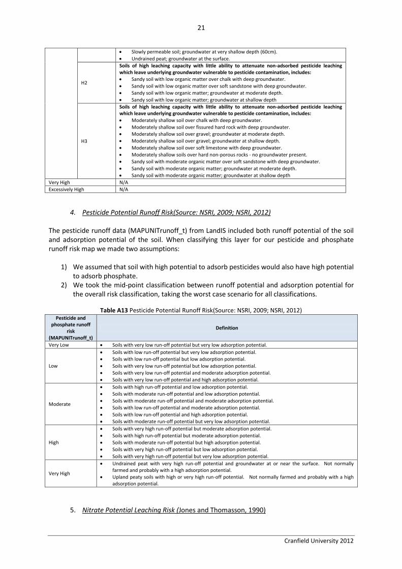
B1: Summary of Land Use and Total SOC (0-150cm) in Central Bedfordshire
Figure B1 Percentage area of Central Bedfordshire within each land use category
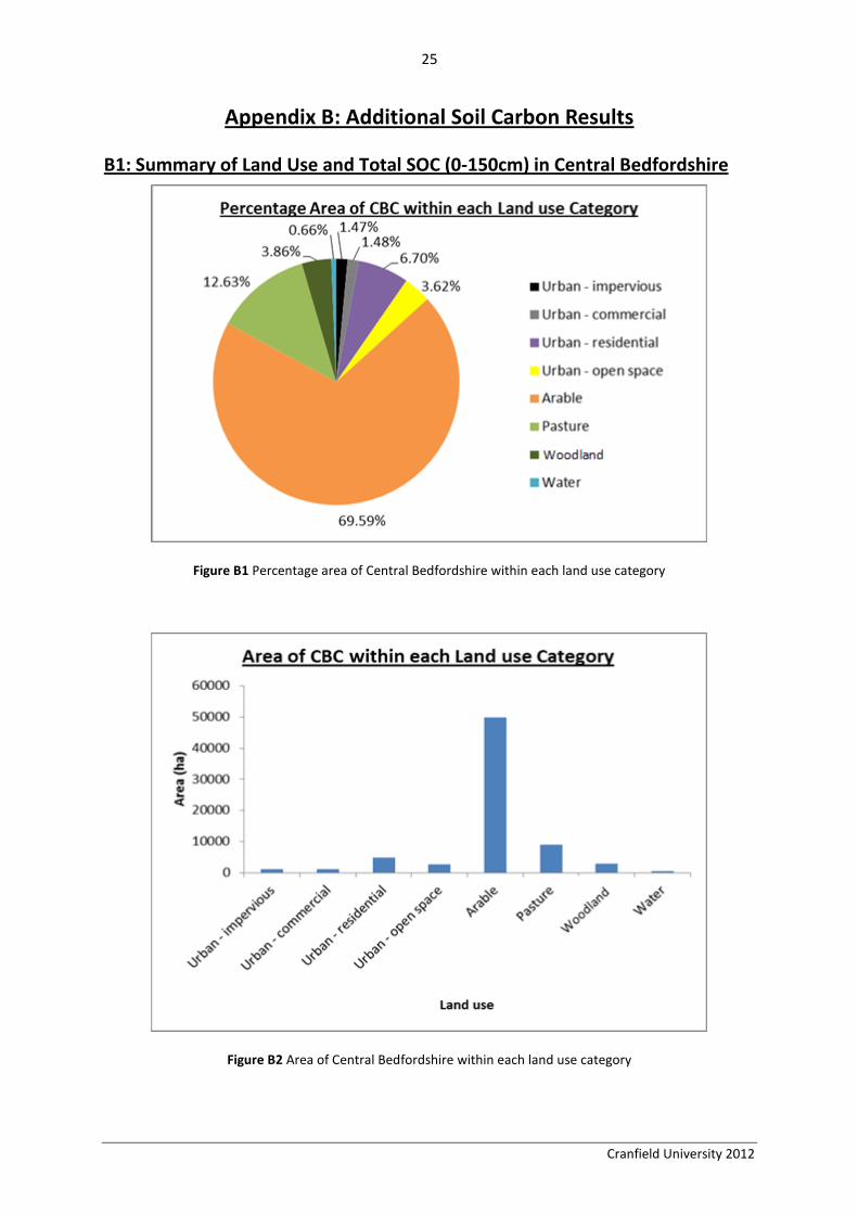
Figure B2 Area of Central Bedfordshire within each land use category

26
Cranfield University 2012
Figure B3 Percentage area of pasture and arable land in Central Bedfordshire under Agri-Environmental
Scheme (EL: Entry level; HL: High level and OL: Organic level)
Figure B4 Percentage area of Central Bedfordshire within each SOC density (t ha-1
) class in the profile 0-150 cm
(excludes water bodies).
34.5 %
9.1%
0.7%
0.2 % 0.9 %
54.5 %
% Area of Pasture and Arable land in CBC under Agri-Environmental Schemes
EL
EL + HL
HL
OL
OL + HL
None

27
Cranfield University 2012
B2: Maps with Land Use and SOC Data combined
Figure B5 Spatial distribution of SOC density in Central Bedfordshire for depths of 0-30 cm by land use

28
Cranfield University 2012
Figure B6 Spatial distribution of SOC density in Central Bedfordshire for depths of 30-100 cm by land use

29
Cranfield University 2012
Figure B7 Spatial distribution of SOC density in Central Bedfordshire for depths of 100-150 cm by land use

30
Cranfield University 2012
B3: Results Tables
Soil carbon storage in different soil types under arable land use
Table B1 Mean, minimum and maximum values of soil carbon density (t ha-1
) in different soil types under arable land use at depth 0-30cm (EL: Entry level; HL: High level
and OL: Organic level environmental stewardship schemes)
Soil type Agri-Environment Scheme
none EL HL EL+HL OL OL+HL
Deep clay 88.33
(82.10,90.60) 87.68
(82.10,90.60) 83.81
(82.10,90.60) 86.19
(82.10,90.60)
90.21 (82.10,90.60)
Deep loam 74.04
(69.90,75.10) 74.29
(69.90,75.10)
73.90 (73.90,73.90)
Deep loam over gravel 58.63
(57.20,59.50) 58.40
(57.20,59.50) 59.50
(57.20,59.50) 59.00
(57.20,59.50)
Deep loam to clay 61.72
(58.10,82.00) 62.21
(58.10,82.00) 58.54
(58.10,60.80) 60.16
(58.10,82.00) 58.1
(58.10,58.10) 60.80
(60.80,60.80)
Deep sandy 66.50
(66.50,66.50) 66.50
(66.50,66.50) 66.50
(66.50,66.50) 66.50
(66.50,66.50)
Deep silty to clay 70.80
(70.80,70.80) 70.80
(70.80,70.80)
70.80 (70.80,70.80)
Loam over chalk 83.26
(69.70,85.30) 84.94
(69.70,85.30)
85.30 (85.30,85.30)
85.30
(85.30,85.30)
Loam over red sandstone 59.50
(59.50,59.50) 59.50
(59.50,59.50) 59.50
(59.50,59.50) 59.50
(59.50,59.50)
59.50 (59.50,59.50)
Seasonally wet deep clay 106.20
(69.20,141.20) 90.47
(69.20,141.20) 141.20
(141.20,141.20) 127.62
(83.00,141.20)
69.20 (69.20,69.20)
Seasonally wet deep peat to loam 225.60
(225.60,225.60) 225.60
(225.60,225.60)
225.60 (225.60,225.60)
Seasonally wet loam over gravel 89.20
(89.20,89.20) 89.20
(89.20,89.20)
89.20 (89.20,89.20)
Shallow silty over chalk 120.12
(85.90,130.70) 120.06
(85.90,130.70) 87.80
(87.80,87.80) 101.93
(87.80,130.70)
90.03 (87.80,130.70)
Silty over chalk 88.50
(88.50,88.50) 88.50
(88.50,88.50)
88.50 (88.50,88.50)

31
Cranfield University 2012
Table B2 Mean, minimum and maximum values of soil carbon density (t ha-1
) in different soil types under arable land use at depth 30-100cm (EL: Entry level; HL: High level
and OL: Organic level environmental stewardship schemes)
Soil type Agri-Environment Scheme
none EL HL EL+HL OL OL+HL
Deep clay 63.87
(51.70,68.30) 62.61
(51.70,68.30) 55.03
(51.70,68.30) 59.68
(51.70,68.30)
67.55 (51.70,68.30)
Deep loam 37.42
(34.70,54.30) 36.57
(34.70,54.30)
34.70 (34.70,34.70)
Deep loam over gravel 32.90
(31.20,35.70) 33.36
(31.20,35.70) 31.20
(31.20,35.70) 32.06
(31.20,35.70)
Deep loam to clay 43.57
(41.00,49.30) 43.89
(41.00,47.60) 45.02
(41.00,45.80) 42.42
(41.00,47.60) 45.80
(45.80,45.80) 41.00
(41.00,41.00)
Deep sandy 29.00
(29.00,29.00) 29.00
(29.00,29.00) 29.00
(29.00,29.00) 29.00
(29.00,29.00)
Deep silty to clay 27.60
(27.60,27.60) 27.60
(27.60,27.60)
27.60 (27.60,27.60)
Loam over chalk 20.70
(20.20,24.00) 20.29
(20.20,24.00)
20.20 (20.20,20.20)
20.20
(20.20,20.20)
Loam over red sandstone 32.00
(32.00,32.00) 32.00
(32.00,32.00) 32.00
(32.00,32.00) 32.00
(32.00,32.00)
32.00 (32.00,32.00)
Seasonally wet deep clay 69.10
(40.10,103.00) 57.17
(40.10,103.00) 88.30
(88.30,88.30) 81.34
(56.60,103.00)
40.10 (40.10,40.10)
Seasonally wet deep peat to loam 300.90
(300.90,300.90) 300.90
(300.90,300.90)
300.90 (300.90,300.90)
Seasonally wet loam over gravel 42.25
(42.50,42.50) 42.50
(42.50,42.50)
42.50 (42.50,42.50)
Shallow silty over chalk 10.52
(5.90,12.40) 10.55
(5.90,12.40) 5.90
(5.90,5.90) 7.86
(5.90,12.40)
6.18 (5.90,12.40)
Silty over chalk 48.50
(48.50,48.50) 48.50
(48.50,48.50)
48.50 (48.50,48.50)

32
Cranfield University 2012
Table B3 Mean, minimum and maximum values of soil carbon density (t ha-1
) in different soil types under arable land use at depth 100-150cm (EL: Entry level; HL: High level
and OL: Organic level environmental stewardship schemes)
Soil type Agri-Environment Scheme
none EL HL EL+HL OL OL+HL
Deep clay 26.43
(22.10,26.80) 26.26
(22.10,26.80) 25.76
(25.50,26.80) 26.12
(25.50,26.80)
26.74 (25.50,26.80)
Deep loam 14.43
(9.40,16.00) 14.49
(9.4,16.00)
9.40 (9.40,9.40)
Deep loam over gravel 5.09
(3.70,7.40) 5.47
(3.70,7.40) 3.70
(3.70,7.40) 4.41
(3.70,7.40)
Deep loam to clay 12.34
(5.10,17.10) 11.86
(6.90,17.10) 8.57
(6.90,17.10) 14.14
(6.90,17.10) 6.90
(6.90,6.90) 17.10
(17.10,17.10)
Deep sandy 2.60
(2.60,2.60) 2.60
(2.60,2.60) 2.60
(2.60,2.60) 2.60
(2.60,2.60)
Deep silty to clay 6.40
(6.40,6.40) 6.40
(6.40,6.40)
6.40 (6.40,6.40)
Loam over chalk 1.31
(0.90,4.00) 0.97
(0.90,4.00)
0.90 (0.90,0.90)
0.90
(0.90,0.90)
Loam over red sandstone 6.10
(6.10,6.10) 6.10
(6.10,6.10) 6.10
(6.10,6.10) 6.10
(6.10,6.10)
6.10 (6.10,6.10)
Seasonally wet deep clay 25.97
(14.40,79.70) 26.46
(14.40,79.70) 34.00
(34.00,34.00) 30.51
(14.40,79.70)
19.60 (19.60,19.60)
Seasonally wet deep peat to loam 137.70
(137.70,137.70) 137.70
(137.70,137.70)
137.70 (137.70,137.70)
Seasonally wet loam over gravel 4.10
(4.10,4.10) 4.10
(4.10,4.10)
4.10 (4.10,4.10)
Shallow silty over chalk 3.25
(0.90,4.40) 3.26
(0.90,4.40) 0.90
(0.90,0.90) 1.92
(0.90,4.40)
1.04 (0.90,4.40)
Silty over chalk 10.50
(10.50,10.50) 10.50
(10.50,10.50)
10.50 (10.50,10.50)

33
Cranfield University 2012
Table B4 Mean, minimum and maximum values of soil carbon density (t ha-1
) in different soil types under arable land use at total depth 0-150cm (EL: Entry level; HL: High
level and OL: Organic level environmental stewardship schemes)
Soil type Agri-Environment Scheme
none EL HL EL+HL OL OL+HL
Deep clay 178.62
(159.30,185.70) 176.55
(159.30,185.70) 164.60
(159.30,185.70) 171.99
(159.30,185.70)
184.50 (159.30,185.70)
Deep loam 125.89
(118.00,137.70) 125.34
(118.00,137.70)
118.00 (118.00,118.00)
Deep loam over gravel 96.62
(94.40,100.30) 97.23
(94.40,100.30) 94.40
(94.40,100.30) 95.53
(94.40,100.30)
Deep loam to clay 117.64
(110.80,140.10) 117.96
(110.80,140.10) 112.12
(110.80,118.90) 116.71
(110.80,140.10) 110.80
(110.80,110.80) 118.90
(118.90,118.90)
Deep sandy 98.10
(98.10,98.10) 98.10
(98.10,98.10) 98.10
(98.10,98.10) 98.10
(98.10,98.10)
Deep silty to clay 104.80
(104.80,104.80) 104.80
(104.80,104.80)
104.80 (104.80,104.80)
Loam over chalk 105.26
(97.70,106.40) 106.20
(97.70,106.40)
106.40 (106.40,106.40)
106.40
(106.40,106.40)
Loam over red sandstone 97.60
(97.60,97.60) 97.60
(97.60,97.60) 97.60
(97.60,97.60) 97.60
(97.60,97.60)
97.60 (97.60,97.60)
Seasonally wet deep clay 201.27
(128.90,314.30) 174.10
(128.90,314.30) 263.50
(263.50,263.50) 239.47
(154.00,314.30)
128.90 (128.90,128.90)
Seasonally wet deep peat to loam 664.40
(664.20,664.20) 664.20
(664.20,664.20)
664.20 (664.20,664.20)
Seasonally wet loam over gravel 135.80
(135.80,135.80) 135.80
(135.80,135.80)
135.80 (135.80,135.80)
Shallow silty over chalk 133.90
(94.60,147.50) 133.88
(94.60,147.50) 94.60
(94.60,94.60) 111.71
(94.60,147.50)
97.24 (94.60,147.50)
Silty over chalk 147.50
(147.50,147.50) 147.50
(147.50,147.50)
147.50 (147.50,147.50)
34
Cranfield University 2012
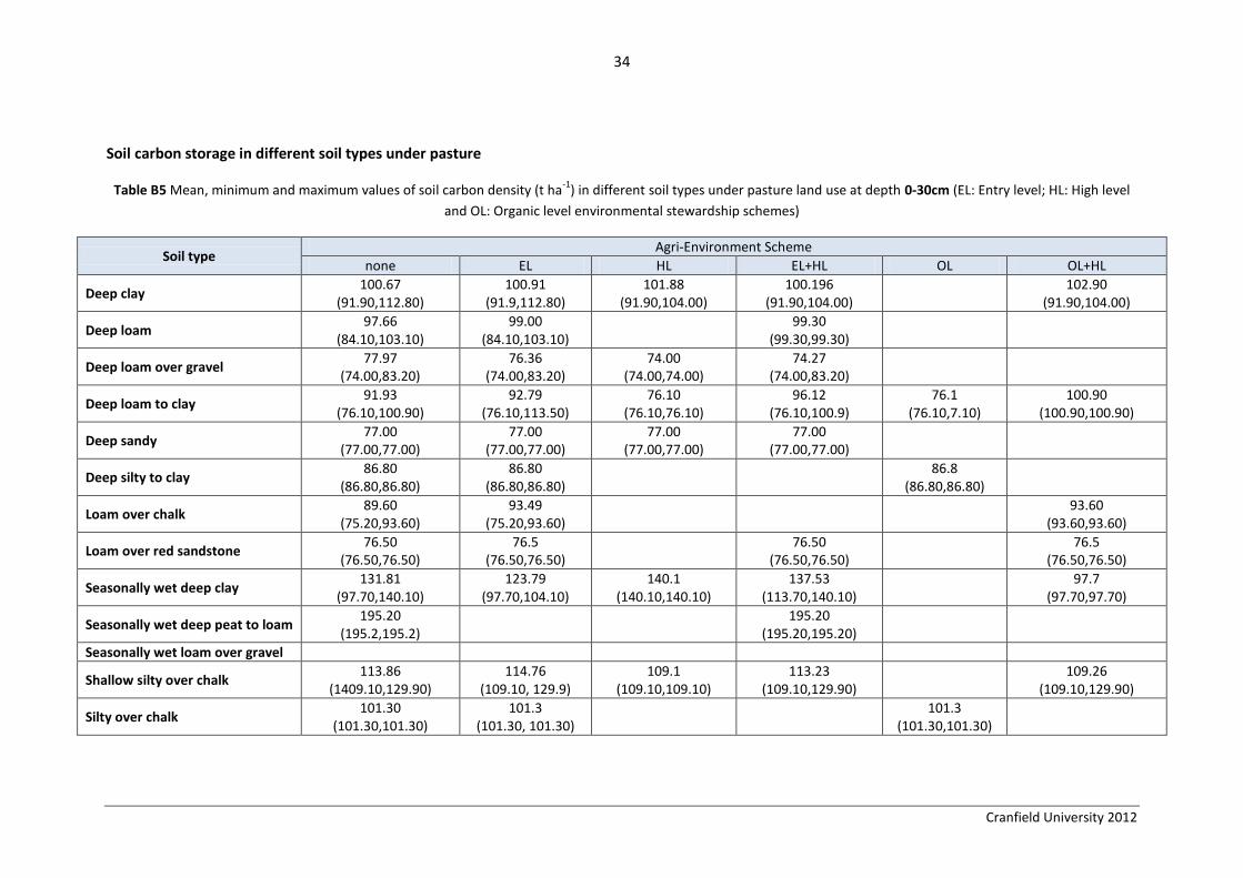
Soil carbon storage in different soil types under pasture
Table B5 Mean, minimum and maximum values of soil carbon density (t ha-1
) in different soil types under pasture land use at depth 0-30cm (EL: Entry level; HL: High level
and OL: Organic level environmental stewardship schemes)
Soil type Agri-Environment Scheme
none EL HL EL+HL OL OL+HL
Deep clay 100.67
(91.90,112.80) 100.91
(91.9,112.80) 101.88
(91.90,104.00) 100.196
(91.90,104.00)
102.90 (91.90,104.00)
Deep loam 97.66
(84.10,103.10) 99.00
(84.10,103.10)
99.30 (99.30,99.30)
Deep loam over gravel 77.97
(74.00,83.20) 76.36
(74.00,83.20) 74.00
(74.00,74.00) 74.27
(74.00,83.20)
Deep loam to clay 91.93
(76.10,100.90) 92.79
(76.10,113.50) 76.10
(76.10,76.10) 96.12
(76.10,100.9) 76.1
(76.10,7.10) 100.90
(100.90,100.90)
Deep sandy 77.00
(77.00,77.00) 77.00
(77.00,77.00) 77.00
(77.00,77.00) 77.00
(77.00,77.00)
Deep silty to clay 86.80
(86.80,86.80) 86.80
(86.80,86.80)
86.8 (86.80,86.80)
Loam over chalk 89.60
(75.20,93.60) 93.49
(75.20,93.60)
93.60 (93.60,93.60)
Loam over red sandstone 76.50
(76.50,76.50) 76.5
(76.50,76.50)
76.50 (76.50,76.50)
76.5
(76.50,76.50)
Seasonally wet deep clay 131.81
(97.70,140.10) 123.79
(97.70,104.10) 140.1
(140.10,140.10) 137.53
(113.70,140.10)
97.7 (97.70,97.70)
Seasonally wet deep peat to loam 195.20
(195.2,195.2)
195.20 (195.20,195.20)
Seasonally wet loam over gravel
Shallow silty over chalk 113.86
(1409.10,129.90) 114.76
(109.10, 129.9) 109.1
(109.10,109.10) 113.23
(109.10,129.90)
109.26 (109.10,129.90)
Silty over chalk 101.30
(101.30,101.30) 101.3
(101.30, 101.30)
101.3 (101.30,101.30)

35
Cranfield University 2012
Table B6 Mean, minimum and maximum values of soil carbon density (t ha-1
) in different soil types under pasture land use at depth 30-100cm (EL: Entry level; HL: High
level and OL: Organic level environmental stewardship schemes)
Soil type Agri-Environment Scheme
none EL HL EL+HL OL OL+HL
Deep clay 69.38
(60.60,75.50) 69.81
(60.60,75,50) 70.91
(60.6,73.10) 69.17
(60.60,73.10)
71.96 (60.60,73.10)
Deep loam 42.51
(40.40,49.70) 43.53
(40.40,49.70)
40.4 (40.40,40.40)
Deep loam over gravel 35.40
(35.10,35.80) 35.28
(35.10,35.80) 35.10
(35.10,31.50) 35.12
(35.10,35.80)
Deep loam to clay 52.78
(48.70,56.10) 52.96
(48.70,56.10) 48.70
(48.70,48.70) 54.67
(48.70,56.10) 48.70
(48.70,48.70) 56.1
(56.10,56.10)
Deep sandy 44.70
(44.70,44.70) 44.70
(44.70,44.70) 44.70
(44.70,44.70) 44.7
(44.70,44.70)
Deep silty to clay 29.40
(29.4,29.4) 29.40
(29.40,29.40)
29.40 (29.40,29.40)
Loam over chalk 21.16
(20.20,24.60) 20.23
(20.20,24.60)
20.20 (20.20,20.20)
Loam over red sandstone 39.00
(39.00,39.00) 39.00
(39.00,39.00)
39.00 (39.00,39.00)
39.00
(39.00,39.00)
Seasonally wet deep clay 112.35
(46.60,130.80) 96.96
(46.60,130.80) 130.8
(130.80,130.80) 122.61
(70.80,130.80)
46.60 (46.60,46.60)
Seasonally wet deep peat to loam 274.70
(274.70,274.70)
274.70 (274.70,274.70)
Seasonally wet loam over gravel
Shallow silty over chalk 8.06
(5.90,15.80) 8.58
(5.90,15.8) 5.90
(5.90,5.90) 7.11
(5.90,12.00)
5.96 (5.90,15.80)
Silty over chalk 49.30
(49.30,49.30) 49.30
(49.30,49.30)
49.3 (49.30,49.3)

36
Cranfield University 2012
Table B7 Mean, minimum and maximum values of soil carbon density (t ha-1
) in different soil types under pasture land use at depth 100-150cm (EL: Entry level; HL: High
level and OL: Organic level environmental stewardship schemes)
Soil type Agri-Environment Scheme
none EL HL EL+HL OL OL+HL
Deep clay 26.22
(22.40,26.80) 26.39
(22.40,26.80) 26.57
(25.50,26.80)
26.39 (25.50,26.80)
26.68
(25.50,26.80)
Deep loam 11.07
(9.40,17.00) 11.01
(9.40,17.00)
9.40 9.40,9.40
Deep loam over gravel 4.53
(4.10,5.10) 4.36
(4.10,5.10) 4.10
(4.10,4.10) 4.13
(4.10,5.10)
Deep loam to clay 12.25
(5.10,17.90) 12.43
(6.90,17.90) 6.90
(6.90,6.90) 15.78
(6.90,17.90) 6.90
(6.90,6.90) 17.90
(17.90,17.90)
Deep sandy 2.60 (2.60,2.60)
2.60 (2.60,2.60)
2.60 (2.60,2.60)
2.60 (2.60,2.60)
Deep silty to clay 6.40
(6.40,6.40) 6.40
(6.40,6.40)
6.40 (6.40,6.40)
Loam over chalk 1.57
(0.90,4.00) 0.92
(0.90,4.00)
0.90 (0.90,0.90)
Loam over red sandstone 6.10
(6.10,6.10) 6.1
(6.10,6.10)
6.10 (6.10,6.10)
6.10
(6.10,6.10)
Seasonally wet deep clay 35.53
(15.70,79.70) 38.03
(15.70,79.70)
51.69 (15.70,79.70)
21.80
(21.80,21.80)
Seasonally wet deep peat to loam 137.70
(137.70,137.70)
30.5 (30.50,30.50)
137.7 (137.70,137.70)
Seasonally wet loam over gravel
Shallow silty over chalk 1.64
(0.90,4.40) 1.83
(0.90,4.40) 0.90
(0.90,0.90) 1.24
(0.90,2.60)
0.92 (0.90,4.40)
Silty over chalk 10.50
(10.50,10.50) 10.50
(10.50,10.50)
10.50 (10.50,10.50)

37
Cranfield University 2012
Table B8 Mean, minimum and maximum values of soil carbon density (t ha-1
) in different soil types under pasture land use at total depth 0-150cm (EL: Entry level; HL: High
level and OL: Organic level environmental stewardship schemes)
Soil type Agri-Environment Scheme
none EL HL EL+HL OL OL+HL
Deep clay 196.27
(178.00,210.70) 197.11
(178.00,210.70) 199.37
(178.00,203.90)
195.76 (178.00,203.90)
201.55
(178.00,203.90)
Deep loam 151.24
(144.30,165.00)
153.53 (144.3,165.00)
149.10
(149.10,149.10)
Deep loam over gravel 117.90
(113.20,124.10) 116.00
(113.20,124.10) 113.20
(113.20,113.20) 113.51
(113.20,124.10)
Deep loam to clay 156.96
(131.70,179.70) 158.18
(131.70,179.70) 131.70
(131.70,131.70) 166.57
(131.70,174.90) 131.70
(131.70,131.70)
174.90 (174.90,174.90)
Deep sandy 124.30
(124.30,124.30) 124.30
(124.30,124.30) 124.30
(124.30,124.30) 124.30
(124.30,124.3)
Deep silty to clay 122.60
(122.60,122.60)
122.60 (122.60,122.60)
122.60
(122.60,122.60)
Loam over chalk 112.33
(103.80,114,70) 114.64
(103.80,114.70)
114.70 (114.70,114.70)
Loam over red sandstone 121.60
(121.60,121.60) 121.60
(121.60,121.60)
121.60 (121.60,121.60)
121.60
(121.60,121.60)
Seasonally wet deep clay 279.69
(166.10,332.20) 258.77
(166.10,332.20)
311.83 (200.20,332.20)
166.10
(166.10,166.10)
Seasonally wet deep peat to loam 607.60
(607.60,607.60)
301.40 (301.40,301.40)
607.60 (607.60,607.60)
Seasonally wet loam over gravel
Shallow silty over chalk 123.56
(115.90,150.00) 125.17
(115.90,150.00) 115.90
(115.90,115.90) 121.58
(115.90,144.50)
116.14 (115.90,150.00)

38
Cranfield University 2012
Silty over chalk 161.10
(161.10,161.10) 161.1
(161.10,161.10)
161.10 (161.10,161.10)
Soil carbon storage in different soil types under woodland vegetation
Table B9 Mean, minimum and maximum values of soil carbon density (t ha-1
) in different soil types under woodland at depth 0-30cm
Soil type woodland type
Broad-leaved Coniferous Mixed Transitional woodland-shrub
Deep clay 119.38
(114.88, 130.00) 121.37
(114.88, 130.00) 125.62
(114.88, 130.00) 130
(122.13, 122.13)
Deep loam 105.13
(105.13, 105.13) 105.13
(105.13, 105.13)
Deep loam over gravel 92.50
(92.5, 92.50) 92.5
(92.50, 92.50)
Deep loam to clay 111.31
(95.13, 126.13) 126.13
(126.13, 126.13)
126.13 (126.13, 126.13)
Deep sandy 96.25
(96.25, 96.25) 96.25
(96.25, 96.25)
Deep silty to clay 108.5
(108.5, 108.5)
Loam over chalk 117
(117.00, 117.00)
117.00 (117.00, 117.00)
Loam over red sandstone 95.63
(95.63, 95.63) 95.63
(95.63, 95.63)
95.63 (95.63, 95.63)
Seasonally wet deep clay 131.19
(122.13, 175.13) 122.45
(122.13, 175.13) 142.13
(142.13, 142.13) 122.13
(112.13, 112.13)
Seasonally wet deep peat to loam 244
(244.00, 244.00)
Seasonally wet loam over gravel
Shallow silty over chalk 136.38
(136.38, 136.38)
147.11 (136.38, 162.38)
Silty over chalk

39
Cranfield University 2012
Table B10 Mean, minimum and maximum values of soil carbon density (t ha-1
) in different soil types under woodland at depth 30-100cm
Soil type Woodland type
Broad-leaved Coniferous Mixed Transitional woodland-shrub
Deep clay 80.41
(75.75, 91.38) 82.46
(75.75, 91.38) 86.85
(75.75, 91.38) 91.38
(91.38, 91.38)
Deep loam 54.00
(54.00, 54.00) 54.00
(54.00, 54.00)
Deep loam over gravel 43.88
(43.88, 43.88) 43.88
(43.88, 43.88)
Deep loam to clay 65.71
(60.88, 70.13) 70.13
(70.13, 70.13)
70.13 (70.13, 70.13)
Deep sandy 55.88
(55.88, 55.88) 55.88
(55.88, 55.88)
Deep silty to clay 36.75
(36.75, 36.75)
Loam over chalk 25.25
(25.25, 25.25)
25.25 (25.25, 25.25)
Loam over red sandstone 48.75
(48.75, 48.75) 48.75
(75.75, 91.38)
48.75 (48.75, 48.75)
Seasonally wet deep clay 74.89
(58.25, 163.50) 58.90
(58.25, 163.50) 88.50
(88.50, 88.50) 58.25
(58.25, 58.25)
Seasonally wet deep peat to loam 343.38
(343.38, 343.38)
Seasonally wet loam over gravel
Shallow silty over chalk 7.38
(7.38, 7.38)
10.52 (7.38, 15.00)
Silty over chalk

40
Cranfield University 2012
Table B11 Mean, minimum and maximum values of soil carbon density (t ha-1
) in different soil types under woodland at depth 100-150cm
Soil type Woodland type
Broad-leaved Coniferous Mixed Transitional woodland-shrub
Deep clay 32.36
(31.88, 33.5) 32.57
(31.88, 32.50) 33.03
(31.88, 33.50) 33.50
(33.50, 33.50)
Deep loam 21.25
(21.25, 21.25) 21.25
(21.25, 21.25)
Deep loam over gravel 5.13
(5.13, 5.13) 5.13
(5.13, 5.13)
Deep loam to clay 15.81
(8.63, 22.38) 22.38
(22.38, 22.38)
22.38 (22.38, 22.38)
Deep sandy 3.25
(3.25, 3.25) 3.25
(3.25, 3.25)
Deep silty to clay 8.00
(8.00, 8.00)
Loam over chalk 1.13
(1.13, 1.13)
1.13 (1.13, 1.13)
Loam over red sandstone 7.63
(7.63, 7.63) 7.63
(7.63, 7.63)
7.63 (7.63, 7.63)
Seasonally wet deep clay 27.42
(19.63, 38.13) 27.32
(27.25, 38.13) 19.63
(19.63, 19.63) 27.25
(27.25, 27.25)
Seasonally wet deep peat to loam 172.13
(172.13, 172.13)
Seasonally wet loam over gravel
Shallow silty over chalk 1.13
1.13, 1.13)
2.00 (1.13, 3.25)
Silty over chalk

41
Cranfield University 2012
Table B12 Mean, minimum and maximum values of soil carbon density (t ha-1
) in different soil types under woodland at total depth 0-150cm
Soil type Woodland type
Broad-leaved Coniferous Mixed Transitional woodland-shrub
Deep clay 232.15
(222.50, 254.88) 236.41
(222.50, 254.88) 245.50
(222.50, 254.88) 254.88
(254.88, 254.88)
Deep loam 180.38
(180.38, 180.38) 180.38
(180.38, 180.30)
Deep loam over gravel 141.50
(141.50, 141.50) 141.50
(141.50, 141.50)
Deep loam to clay 192.82
(164.63, 218.63) 218.63
(218.63, 218.63)
218.63 (218.63, 218.63)
Deep sandy 155.38
(155.38, 155.38) 155.38
(155.38, 155.38)
Deep silty to clay 153.25
(153.25, 153.25)
Loam over chalk 143.38
(143.38, 143.38)
143.38 (143.38, 143.38)
Loam over red sandstone 152.00
(152.00, 152.00) 152.00
(152.00, 152.00)
152.00 (152.00, 152.00)
Seasonally wet deep clay 233.50
(376.75, 207.63) 208.66
(207.63, 176.75) 250.25
(250.25, 250.25) 207.63
(207.63, 207.63)
Seasonally wet deep peat to loam 759.50
(759.50, 759.50)
Seasonally wet loam over gravel
Shallow silty over chalk 144.88
(144.88, 144.88)
159.63 (144.88, 180.63)
Silty over chalk

42
Cranfield University 2012
Soil carbon storage in different soil types under urban land use
Table B13 Mean, minimum and maximum values of soil carbon density (t ha-1
) in different soil types under urban land use at depth 0-30cm
Soil type Urban
Commercial Residential Impervious Open spaces
Deep clay 15.4
(13.8.16.9) 35.7
(35.2, 39.5) 0.0
(0.0, 0.0) 87.7
(82.7,93.6)
Deep loam 12.6
(12.6,12.6) 32.5
(29.4,34.8) 0.0
(0.0, 0.0) 89.4
(89.4,89.4)
Deep loam over gravel 11.1
(11.1,11.1) 26.5
(25.9,29.1) 0.0
(0.0, 0.0) 71.4
(66.6,74.9)
Deep loam to clay 16.9
(15.1.17.0) 31.5
(26.6,39.7) 0.0
(0.0, 0.0) 76.3
(68.5,102.2)
Deep sandy 11.6
(11.6,11.6) 27.0
(27.0,27.0) 0.0
(0.0, 0.0) 69.3
(69.3,69.3)
Deep silty to clay 0.0
(0.0, 0.0)
Loam over chalk 14.0
(14.0,14.0) 32.8
(26.3,32.8) 0.0
(0.0, 0.0) 84.2
(84.2,84.2)
Loam over red sandstone 11.5
(11.5,11.5) 26.8
(26.8,26.8) 0.0
(0.0, 0.0) 68.9
(68.9,68.9)
Seasonally wet deep clay 19.2
(10.6,19.6) 44.5
(16.3,45.8) 0.0
(0.0, 0.0) 91.8
(87.9,126.1)
Seasonally wet deep peat to loam 68.3
(68.3,68.3) 0.0
(0.0, 0.0) 175.7
(175.7,175.7)
Seasonally wet loam over gravel 37.3
(37.3,37.3) 0.0
(0.0, 0.0)
Shallow silty over chalk 17.1
(16.4,19.5) 43.1
(38.2,45.5) 0.0
(0.0, 0.0) 105.0
(98.2,116.9)
Silty over chalk 35.5
(35.5.35.5) 0.0
(0.0, 0.0) 91.2
(91.2,91.2)

43
Cranfield University 2012
Table B14 Mean, minimum and maximum values of soil carbon density (t ha-1
) in different soil types under urban land use at depth 30-100cm
Soil type Urban
Commercial Residential Impervious Open spaces
Deep clay 10.8
(9.1,11.3) 24.7
(21.2,26.4) 0.0
(0.0, 0.0) 59.7
(54.5,65.8)
Deep loam 6.5
(6.5,6.5) 14.5
(14.1,15.1) 0.0
(0.0, 0.0) 36.4
(36.4,36.4)
Deep loam over gravel 5.3
(5.3,5.3) 12.3
(12.2,12.5) 0.0
(0.0, 0.0) 32.0
(31.6,32.2)
Deep loam to clay 8.3
(8.2,8.4) 18.4
(17.0,19.6) 0.0
(0.0, 0.0) 45.9
(43.8,50.5)
Deep sandy 6.7
(6.7,6.7) 15.6
(15.6,15.6) 0.0
(0.0, 0.0) 40.2
(40.2,40.2)
Deep silty to clay 0.0
(0.0, 0.0)
Loam over chalk 3.0
(3.0,3.0) 7.1
(7.0,8.6) 0.0
(0.0, 0.0) 18.2
(18.2,18.2)
Loam over red sandstone 5.9
(5.9,5.9) 13.7
(13.7,13.7) 0.0
(0.0, 0.0) 35.1
(35.1,35.1)
Seasonally wet deep clay 15.1
(10.6,19.6) 35.9
(16.3,45.8) 0.0
(0.0, 0.0) 49.6
(41.9,117.72)
Seasonally wet deep peat to loam 96.1
(96.1.96.1) 0.0
(0.0, 0.0) 247.2
(247.2,247.2)
Seasonally wet loam over gravel 15.4
(15.4,15.4) 0.0
(0.0, 0.0)
Shallow silty over chalk 1.2
(0.9,2.4) 4.3
(2.1,5.5) 0.0
(0.0, 0.0) 8.5
(5.3,14.2)
Silty over chalk 17.3
(17.3,17.3) 0.0
(0.0, 0.0) 44.4
(44.4,44.4)

44
Cranfield University 2012
Table B15 Mean, minimum and maximum values of soil carbon density (t ha-1
) in different soil types under urban land use at depth 100-150cm
Soil type Urban
Commercial Residential Impervious Open spaces
Deep clay 4.0
(3.4,4.0) 9.2
(7.8,9.4) 0.0
(0.0, 0.0) 23.5
(23.0,24.1)
Deep loam 2.6
(2.6,2.6) 4.4
(3.3,6.0) 0.0
(0.0, 0.0) 8.5
(8.5,8.5)
Deep loam over gravel 0.6
(0.6,0.6) 1.5
(1.4,1.8) 0.0
(0.0, 0.0) 4.2
(3.7,4.6)
Deep loam to clay 1.7
(1.7,2.7) 4.2
(2.4,6.3) 0.0
(0.0, 0.0) 9.0
(6.2,16.1)
Deep sandy 0.4
(0.4,0.4) 0.9
(0.9,0.9) 0.0
(0.0, 0.0) 2.3
(2.3,2.3)
Deep silty to clay - - 0.0
(0.0, 0.0) -
Loam over chalk 0.1
(0.1,0.1) 0.3
(0.3,1.4) 0.0
(0.0, 0.0) 0.8
(0.8,0.8)
Loam over red sandstone 0.9
(0.9,0.9) 2.1
(2.1,2.1) 0.0
(0.0, 0.0) 5.5
(5.5,5.5)
Seasonally wet deep clay 6.1
(2.4,12.0) 12.7
(5.5,27.9) 0.0
(0.0, 0.0) 20.4
(19.6,27.5)
Seasonally wet deep peat to loam - 48.2
(48.2,48.2) 0.0
(0.0, 0.0) 123.9
(123.9,123.9)
Seasonally wet loam over gravel - 1.4
(1.4,1.4) 0.0
(0.0, 0.0) -
Shallow silty over chalk 0.3
(0.1,0.7) 1.1
(0.3,1.5) 0.0
(0.0, 0.0) 1,9
(0.8,4.0)
Silty over chalk - 3.7
(3.7.3.7) 0.0
(0.0, 0.0) 9.5
(9.5,9.5)

45
Cranfield University 2012
Table B16 Mean, minimum and maximum values of soil carbon density (t ha-1
) in different soil types under urban land use at total depth 0-150cm
Soil type Urban
Commercial Residential Impervious Open spaces
Deep clay 30.2
(26.7,31.6) 69.7
(62.3,73.7) 0.0
(0.0, 0.0) 170.9
(160.2,183.5)
Deep loam 21.6
(21.6.21.6) 51.5
(50.5,52.2) 0.0
(0.0, 0.0) 134.2
(134.2,134.2)
Deep loam over gravel 17.0
(17.0,17.0) 40.4
(39.6.43.4) 0.0
(0.0, 0.0) 107.6
(101.9,111.7)
Deep loam to clay 26.9
(26.2,27.0) 54.1
(46.1,62.9) 0.0
(0.0, 0.0) 131.1
(118.5,161.7)
Deep sandy 18.6
(18.6,18.6) 43.5
(43.5,43.5) 0.0
(0.0, 0.0) 111.9
(111.9,111.9)
Deep silty to clay 0.0
(0.0, 0.0)
Loam over chalk 17.2
(17.2,17.2) 40.1
(36.3,40.1) 0.0
(0.0, 0.0) 103.2
(103.2,103.2)
Loam over red sandstone 18.2
(18.2,18.2) 42.6
(42.6,42.6) 0.0
(0.0, 0.0) 109.4
(109.4,109.4)
Seasonally wet deep clay 40.4
(30.0,49.8) 93.1
(58.1,116.3) 0.0
(0.0, 0.0) 161.9
(149.5,271.3)
Seasonally wet deep peat to loam 212.7
(212.7,212.7) 0.0
(0.0, 0.0) 115.4
(104.3,135.0)
Seasonally wet loam over gravel 54.2
(54.2,54.2) 0.0
(0.0, 0.0)
Shallow silty over chalk 18.6
(17.4,22.5) 48.5
(40.6,52.5) 0.0
(0.0, 0.0) 115.4
(104.3,135.0)
Silty over chalk 56.4
(56.4,56.4) 0.0
(0.0, 0.0) 145.0
(145.0,145.0)

46
Cranfield University 2012

47
Cranfield University 2012
Appendix C: Additional Run-off Results
C1: Scenario Maps
1. Scenario 1: Urban development
Figure C1. Predicted runoff in Central Bedfordshire for the 1 in 10 years storm event under urban land
use. Previous soil wetness was assumed to be intermediate. Potential development sites proposed by
CBC are shown in the map.

48
Cranfield University 2012
Figure C2. Predicted runoff in Central Bedfordshire for the 1 in 100 years storm event under urban land
use. Previous soil wetness was assumed to be intermediate. Potential development sites proposed by
CBC are shown in the map.

49
Cranfield University 2012
Figure C3. Predicted soil loss in Central Bedfordshire County under urban land use. Potential
development sites proposed by CBC are shown in the map.

50
Cranfield University 2012
2. Scenario 2: Woodland land use
Figure C4. Predicted runoff in Central Bedfordshire for the 1 in 10 years storm event under woodland
land use. Previous soil wetness was assumed to be intermediate. Current urban areas stay as urban
areas in this scenario.

51
Cranfield University 2012
Figure C5. Predicted runoff in Central Bedfordshire for the 1 in 100 years storm event under woodland
land use. Previous soil wetness was assumed to be intermediate. Current urban areas stay as urban
areas in this scenario.

52
Cranfield University 2012
Figure C6. Predicted soil loss in Central Bedfordshire under woodland land use. Current urban areas stay
as urban areas in this scenario.

53
Cranfield University 2012
3. Scenario 3: Pasture land use
Figure C7. Predicted runoff in Central Bedfordshire for the 1 in 10 years storm event under pasture land
use. Previous soil wetness was assumed to be intermediate. Current urban areas stay as urban areas in
this scenario.
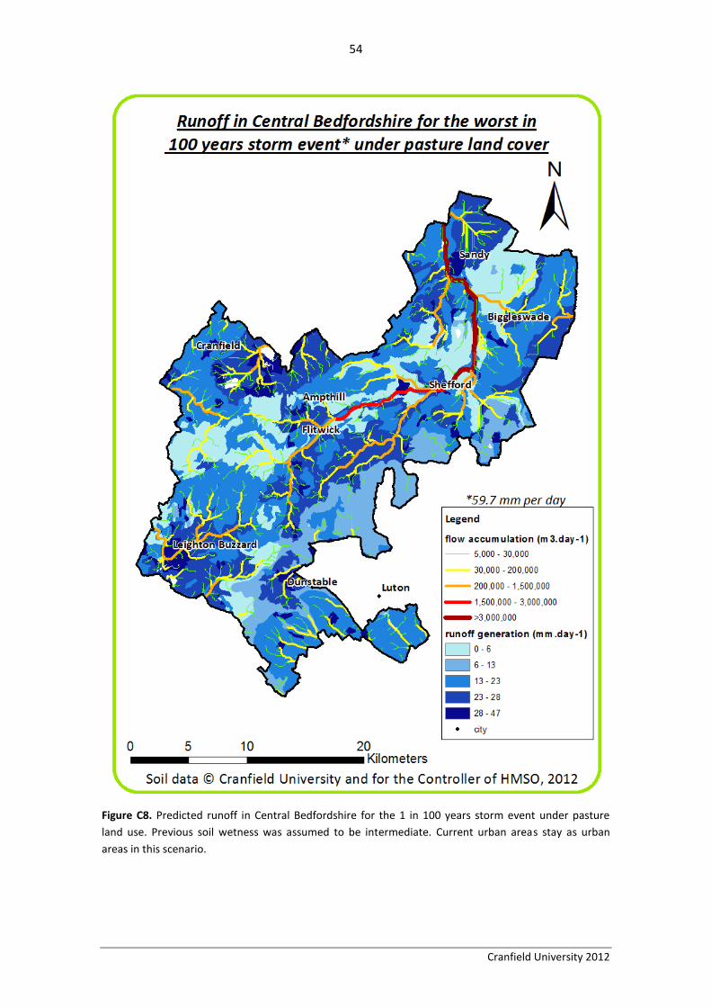
54
Cranfield University 2012
Figure C8. Predicted runoff in Central Bedfordshire for the 1 in 100 years storm event under pasture
land use. Previous soil wetness was assumed to be intermediate. Current urban areas stay as urban
areas in this scenario.

55
Cranfield University 2012
Figure C9. Predicted soil loss in Central Bedfordshire under pasture land use. Current urban areas stay as
urban areas in this scenario.

56
Cranfield University 2012
4. Scenario 4: Implementation of the Biodiversity Action Plan (BAP)
Figure C10. Predicted runoff in Central Bedfordshire for the 1 in 10 years storm event whit
implementation of the BAP. Previous soil wetness was assumed to be intermediate.

57
Cranfield University 2012
Figure C11. Predicted runoff in Central Bedfordshire for the 1 in 100 years storm event whit
implementation of the BAP. Previous soil wetness was assumed to be intermediate.

58
Cranfield University 2012
Figure C12. Predicted soil loss in Central Bedfordshire with implementation of the BAP.

59
Cranfield University 2012
5. Scenario 5: Implementation of good land management techniques
Figure C13. Predicted runoff in Central Bedfordshire for the 1 in 10 years storm event whit
implementation of good land management techniques to prevent erosion and runoff in arable land.
Such land management techniques are specified in the methodology of the scenario. Previous soil
wetness was assumed to be intermediate.

60
Cranfield University 2012
Figure C14. Predicted runoff in Central Bedfordshire for the 1 in 100 years storm event whit
implementation of good land management techniques to prevent erosion and runoff in arable land.
Such land management techniques are specified in the methodology of the scenario. Previous soil
wetness was assumed to be intermediate.

61
Cranfield University 2012
Figure C15. Predicted soil loss in Central Bedfordshire with implementation of the good land
management techniques to prevent erosion and runoff in arable land. Such land management
techniques are specified in the methodology of the scenario.

62
Cranfield University 2012
C2: Scenario Result tables
1. Scenario 1: Widespread urban development
Table C1. Mean runoff predicted (42.6 mm day-1
) after the 1 in 10 years rainfall event for urban development throughout the entire Central Bedfordshire. Values on the
table are interpreted as follow: mean runoff estimated for each combination of land use and Hydrologic soil group (standard deviation – SD- for each combination of land
use and soil type). Current proportion of the different urban land covers within Central Bedfordshire was assigned to the new urban development in order to estimate its
behaviour against runoff.
NEW URBAN DEVELOPMENT CURRENT URBAN DEVELOPMENT
Soil type Weighted urban area Residential areas Impervious Industrial or commercial Open spaces
A 5.4 (2.12) 7.3 (0.82) 4.3 (0.72) 19.5 (0.92) 0.2 (0.7)
B 12.7 (2.53) 14.4 (0.37) 11.4 (0.48) 24.2 (0.43) 3.1 (0.32)
C 17.9 (2.02) 20.9 (0.83) 16.8 (0.71) 27.8 (0.78) 9.2 (0.38)
D 22.6 (1.74) 24.1(0.84) 19.5 (0.15) 29.9 (0.48) 13.7 (1.14)
Table C2. Mean runoff predicted (59.7mm day-1
) after the 1 in 100 years rainfall event for urban development throughout the entire Central Bedfordshire. Values on the
table are interpreted as follow: mean runoff estimated for each combination of land use and Hydrologic soil group (standard deviation – SD- for each combination of land
use and soil type). Current proportion of the different urban land covers within Central Bedfordshire was assigned to the new urban development in order to estimate its
behaviour against runoff.
NEW URBAN DEVELOPMENT CURRENT URBAN DEVELOPMENT
Soil type Weighted urban area Residential areas Impervious Industrial or commercial Open spaces
A 13.1 (4) 16.5 (1.16) 11.5 (1.08) 33.7 (1.24) 0.6 (1.35)
B 24.4 (3.61) 26.9 (0.56) 22.6 (0.68) 39.4 (0.58) 9.4 (0.51)
C 31.5 (2.77) 35.4 (1.14) 30.0 (1.05) 43.8 (0.97) 19.3 (0.74)
D 37.5 (2.17) 39.4 (1.13) 33.6 (0.21) 46.1 (0.58) 25.9 (1.97)

63
Cranfield University 2012
Table C3. Mean erosion predicted (ton ha-1
year-1
) for urban development through the entire county. Values on the table are interpreted as follow: mean erosion for each
combination of land use and soil type (standard deviation – SD- for each combination of land use and soil type). NA (Not Applicable) means that a certain combination of
land use and soil type does not appear in the area. Current proportion of the different urban land covers within Central Bedfordshire was assigned to the new urban
development in order to estimate its behaviour against erosion.
NEW URBAN DEVELOPMENT CURRENT URBAN DEVELOPMENT
Soil type Weighted urban area Residential areas Impervious Industrial or commercial Open spaces
deep clay 33.5 (22.31) 1.0 (7.27) 150.3 (32.55) 1.0 (6.18) 8.5 (14.25)
deep loam 18.3 (6.27) 0.4 (2.52) 45.8 (1.61) 0.9 (5.11) 9.1 (15.11)
deep loam over gravel 13.6 (13.07) 0.4 (3.73) 27.9 (12.34) 0.7 (3.99) 2.8 (8.61)
deep loam to clay 47.6 (63.45) 1.7 (11.28) 639.0 (208.09) 0.9 (5.16) 13.4 (9.75)
deep sandy 41.6 (56.35) 0.9 (6.87) 252.8 (160.57) 1.6 (3.15) 10.0 (4.65)
deep silty to clay NA NA NA NA NA
loam over chalk 20.1 (20.17) 0.2 (3.65) 2.2 (20.39) 0.3 (3.72) 1.8 (9.01)
loam over red sandstone 23.6 (13.07) 0.7 (5.32) NA 0.8 (4.96) 5.7 (4.43)
seasonally wet deep clay 37.9 (57.12) 0.9 (6.93) 231.0 (116.96) 0.7 (4.34) 9.4 (3.44)
seasonally wet deep peat to loam 3.7 (2.13) 0.6 (1.67) 2.1 (1.55) NA 0.7 (1.15)
seasonally wet loam over gravel 4.4 (1.56) 0.2 (1.4) NA NA NA
shallow silty over chalk 54.9 (63.56) 1.6 (13.76) 325.5 (306.26) 0.7 (4.57) 18.3 (30.06)
silty over chalk 110.4 (175.08) 0.2 (0.57) 1115.2 (104.49) NA 10.8 (42.05)

64
Cranfield University 2012
2. Scenario 2: Woodland land use
Table C4. Mean runoff predicted (mm day-1
) in Central Bedfordshire under woodland land use after the 1 in 10 years rainfall event. Current urban areas stay in the same
place. Values on the table are interpreted as follow: mean runoff estimated for each combination of land use and Hydrologic soil group (standard deviation – SD- for each
combination of land use and soil type).
URBAN AREAS NON-URBAN AREAS
Soil type Residential areas Impervious Industrial or commercial Open spaces Woodland
A 7.3 (0.82) 4.3 (0.72) 19.5 (0.92) 0.2 (0.7) 5.0 (0.01)
B 14.4 (0.37) 11.4 (0.48) 24.2 (0.43) 3.1 (0.32) 0.6 (0.02)
C 20.9 (0.83) 16.8 (0.71) 27.8 (0.78) 9.2 (0.38) 4.8 (0.02)
D 24.1 (0.84) 19.5 (0.15) 29.9 (0.48) 13 (1.64) 9.6 (0.02)
Table C5. Mean runoff predicted (mm d-1
) in Central Bedfordshire under woodland land use after the 1 in 100 years rainfall event and. Current urban areas stay in the same
place. Values on the table are interpreted as follow: mean runoff estimated for each combination of land use and Hydrologic soil group (standard deviation – SD- for each
combination of land use and soil type).
URBAN AREAS NON-URBAN AREAS
Soil type Residential areas Impervious Industrial or commercial Open spaces Woodland
A 16.5 (1.16) 11.5 (1.08) 33.7 (1.24) 0.6 (1.35) 1.8 (0.07)
B 26.9 (0.56) 22.6 (0.68) 39.4 (0.58) 9.4 (0.51) 0.1 (0.05)
C 35.4 (1.14) 30.0 (1.05) 43.8 (0.97) 19.3 (0.74) 12.4 (0.04)
D 39.4 (1.13) 33.6 (0.21) 46.1 (0.58) 24.9 (2.6) 20.0 (0.05)

65
Cranfield University 2012
Table 6. Mean erosion predicted (ton ha-1
year-1
) in Central Bedfordshire under woodland land use. Current urban areas stay in the same place. Values on the table are
interpreted as follow: mean erosion for each combination of land use and soil type (standard deviation – SD- for each combination of land use and soil type). NA means
that a certain combination of land use and soil type does not appear in the area.
URBAN AREAS NON-URBAN AREAS
Soil type Residential areas Impervious Industrial or commercial Open spaces Woodland
deep clay 1.0 (7.27) 150.3 (32.55) 1.0 (6.18) 8.5 (14.25) 0.3 (0.15)
deep loam 0.4 (2.52) 45.8 (1.61) 0.9 (5.11) 9.1 (15.11) 0.2 (0.04)
deep loam over gravel 0.4 (3.73) 27.9 (12.34) 0.7 (3.99) 2.8 (8.61) 0.1 (0.11)
deep loam to clay 1.7 (11.28) 639.0 (208.09) 0.9 (5.16) 13.4 (9.75) 0.4 (0.23)
deep sandy 0.9 (6.87) 252.8 (160.57) 1.6 (3.15) 10.0 (4.65) 0.4 (0.17)
deep silty to clay NA NA NA NA 0.3 (0.07)
loam over chalk 0.2 (3.65) 2.2 (20.39) 0.3 (3.72) 1.8 (9.01) 0.3 (0.11)
loam over red sandstone 0.7 (5.32) NA 0.8 (4.96) 5.7 (4.43) 0.2 (0.09)
seasonally wet deep clay 0.9 (6.93) 231.0 (116.96) 0.7 (4.34) 9.4 (3.44) 0.3 (0.21)
seasonally wet deep peat to loam 0.6 (1.67) 2.1 (1.55) NA 0.7 (1.15) NA
seasonally wet loam over gravel 0.2 (1.4) NA NA NA NA
shallow silty over chalk 1.6 (13.76) 325.5 (306.26) 0.7 (4.57) 18.3 (30.06) 0.5 (0.43)
silty over chalk 0.2 (0.57) 1115.2 (104.49) NA 10.8 (42.05) NA

66
Cranfield University 2012
3. Scenario 3: Pasture land use
Table C7. Mean runoff predicted (mm day-1
) in Central Bedfordshire under pasture land use after the 1 in 10 years rainfall event. Current urban areas stay in the same
place. Values on the table are interpreted as follow: mean runoff estimated for each combination of land use and Hydrologic soil group (standard deviation – SD- for each
combination of land use and soil type(See Table A.4).
URBAN AREAS NON-URBAN AREAS
Soil type Residential areas Impervious Industrial or commercial Open spaces Pasture
A 7.3 (0.82) 4.3 (0.72) 19.5 (0.92) 0.2 (0.7) 0.2 (0.1)
B 14.4 (0.37) 11.4 (0.48) 24.2 (0.43) 3.1 (0.32) 1.5 (0.15)
C 20.9 (0.83) 16.8 (0.71) 27.8 (0.78) 9.2 (0.38) 11.3 (0.08)
D 24.1 (0.84) 19.5 (0.15) 29.9 (0.48) 13.7 (1.14) 15.2 (0.08)
Table C8. Mean runoff predicted (mm day-1
) in Central Bedfordshire under pasture land use after the 1 in 100 years rainfall event. Current urban areas stay in the same
place. Values on the table are interpreted as follow: mean runoff estimated for each combination of land use and Hydrologic soil group (standard deviation – SD- for each
combination of land use and soil type).
URBAN AREAS NON-URBAN AREAS
Soil type Residential areas Impervious Industrial or commercial Open spaces Pasture
A 16.5 (1.16) 11.5 (1.08) 33.7 (1.24) 0.6 (1.35) 2.7 (0.19)
B 26.9 (0.56) 22.6 (0.68) 39.4 (0.58) 9.4 (0.51) 6.2 (0.25)
C 35.4 (1.14) 30.0 (1.05) 43.8 (0.97) 19.3 (0.74) 22.4 (0.11)
D 39.4 (1.13) 33.6 (0.21) 46.1 (0.58) 25.9 (1.97) 28.0 (0.12)

67
Cranfield University 2012
Table C9. Mean erosion predicted (ton ha-1
year-1
) in Central Bedfordshire under pasture land use. Current urban areas stay at the same place. Values on the table are
interpreted as follow: mean erosion for each combination of land use and soil type (standard deviation – SD- for each combination of land use and soil type). 0 means that
a certain combination of land use and soil type does not appear in the area.
URBAN AREAS NON-URBAN AREAS
Soil type Residential areas Impervious Industrial or commercial Open spaces Pasture
deep clay 1.0 (7.27) 150.3 (32.55) 1.0 (6.18) 8.5 (14.25) 7.4 (3.4)
deep loam 0.4 (2.52) 45.8 (1.61) 0.9 (5.11) 9.1 (15.11) 4.0 (1.04)
deep loam over gravel 0.4 (3.73) 27.9 (12.34) 0.7 (3.99) 2.8 (8.61) 3.3 (2.68)
deep loam to clay 1.7 (11.28) 639.0 (208.09) 0.9 (5.16) 13.4 (9.75) 9.7 (5.69)
deep sandy 0.9 (6.87) 252.8 (160.57) 1.6 (3.15) 10.0 (4.65) 9.3 (4.18)
deep silty to clay NA NA NA NA 6.8 (2.18)
loam over chalk 0.2 (3.65) 2.2 (20.39) 0.3 (3.72) 1.8 (9.01) 7.4 (2.9)
loam over red sandstone 0.7 (5.32) NA 0.8 (4.96) 5.7 (4.43) 5.8 (2.23)
seasonally wet deep clay 0.9 (6.93) 231.0 (116.96) 0.7 (4.34) 9.4 (3.44) 6.5 (5.2)
seasonally wet deep peat to loam 0.6 (1.67) 2.1 (1.55) NA 0.7 (1.15) 0.8 (0.44)
seasonally wet loam over gravel 0.2 (1.4) NA NA NA NA
shallow silty over chalk 1.6 (13.76) 325.5 (306.26) 0.7 (4.57) 18.3 (30.06) 12.7 (10.65)
silty over chalk 0.2 (0.57) 1115.2 (104.49) NA 10.8 (42.05) 18.0 (6.46)

68
Cranfield University 2012
4. Scenario 4: Biodiversity Action Plan (BAP)
Table C10. Mean runoff predicted (mm day-1
) in Central Bedfordshire under implementation of the BAP use after the 1 in 10 years rainfall event. Values on the table are
interpreted as follow: mean runoff estimated for each combination of land use and Hydrologic soil group (standard deviation – SD- for each combination of land use and
soil type).
URBAN AREAS NON-URBAN AREAS
Soil type Residential areas Impervious Industrial or commercial
Open spaces Pasture Arable land Woodland
A 7.1 (1.48) 4.1 (1.26) 18.25 (4.48) 0.4 (1.23) 0.7 (1.88) 1.5 (1.04) 4.5 (1.15)
B 14.2 (1.84) 11.0 (1.98) 23.8 (2.82) 3.0 (1.12) 1.8 (1.72) 4.0 (0.75) 1.4 (2.47)
C 20.6 (1.94) 15.8 (3.26) 27.4 (3.02) 9.1 (0.92) 11.1 (1.85) 12.6 (1.02) 5.4 (1.56)
D 23.9 (1.85) 18.9 (2.19) 29.3 (3.24) 13.6 (1.12) 15.0 (1.7) 16.9 (0.98) 10.1 (2.46)
Table C11. Mean runoff predicted (mm day-1
) in Central Bedfordshire with implementation of the BAP use after the 1 in 100 years rainfall event. Values on the table are
interpreted as follow: mean runoff estimated for each combination of land use and Hydrologic soil group (standard deviation – SD- for each combination of land use and
soil type).
URBAN AREAS NON-URBAN AREAS
Soil type Residential areas Impervious Industrial or
commercial Open spaces Pasture Arable land Woodland
A 15.9 (3.03) 10.6 (3) 31.0 (8.73) 0.8 (1.65) 3.2 (3.02) 5.8 (1.71) 2.1 (2.53)
B 26.5 (2.98) 22.0 (3.59) 38.9 (4.58) 8.9 (2.31) 6.5 (3.08) 11.0 (1.44) 2.8 (5.36)
C 35.0 (2.71) 28.6 (5.03) 43.2 (4.09) 19.3 (1.47) 22.2 (3) 24.3 (1.59) 13.2 (2.7)
D 39.0 (2.49) 32.9 (3.01) 45.4 (4.13) 25.7 (1.7) 27.8 (2.64) 30.2 (1.41) 20.6 (3.81)

69
Cranfield University 2012
Table C12. Mean erosion predicted (ton ha-1
year-1
) in Central Bedfordshire with implementation of the BAP. Values on the table are interpreted as follow: mean erosion
for each combination of land use and soil type (standard deviation – SD- for each combination of land use and soil type). 0 means that a certain combination of land use
and soil type does not appear in the area.
URBAN AREAS NON-URBAN AREAS
Soil type Residential areas Impervious Industrial or commercial Open spaces Pasture Arable land Woodland
deep clay 1.0 (7.06) 150.0 (33.33) 1.1 (6.9) 3.7 (7.91) 9.4 (11.4) 6.9 (2.18) 9.6 (13.5)
deep loam 0.4 (2.41) 45.8 (2.2) 0.9 (4.85) 9.8 (14.37) 3.3 (1.41) 4.0 (0.93) 5.1 (3.16)
deep loam over gravel 0.4 (3.62) 28.1 (12.51) 0.6 (3.33) 2.8 (8.53) 5.3 (4.6) 2.9 (2.13) 2.8 (2.17)
deep loam to clay 1.7 (10.41) 398.1 (69.33) 0.9 (5.21) 11.8 (8.82) 34.7 (143.39) 9.5 (3.77) 12.1 (28.02)
deep sandy 0.9 (7.16) 220.9 (135.45) 6.1 (24.64) 9.4 (4.23) 22.5 (72.7) 6.9 (3.3) 15.6 (37.11)
deep silty to clay NA NA NA NA 6.6 (3.07) 7.0 (0.05) 5.6 (0.55)
loam over chalk 0.2 (3.16) 1.0 0.3 (3.8) 1.5 (7.57) 6.6 (6.82) 7.3 (2.26) 6.0 (5.88)
loam over red sandstone 0.6 (4.19) NA 0.7 (4.19) 3.6 (4.68) 4.3 (2.4) 5.4 (1.52) 6.0 (2.95)
seasonally wet deep clay 0.9 (6.46) 122.7 (136.16) 0.5 (5.03) 1.3 (2.84) 4.5 (27.26) 5.9 (4.59) 33.8 (79.59)
seasonally wet deep peat to loam 0.7 (1.9) 2.1 (1.58) NA 0.7 (1.15) 0.9 (0.45) 0.8 (0.34) 0.9 (0.85)
seasonally wet loam over gravel 0.2 (1.31) NA NA NA NA 1.0 (0.3) NA
shallow silty over chalk 1.3 (8.97) 150.7 (13.85) 0.7 (4.58) 7.8 (6.52) 26.7 (66.06) 7.4 (5.46) 33.3 (83.4)
silty over chalk 0.2 (0.54) NA NA 10.9 (42.05) 87.3 (269.52) 16.1 (2.10) NA

70
Cranfield University 2012
5. Scenario 5: Implementation of management techniques in arable land
Table C13. Mean runoff predicted (mm day-1
) in Central Bedfordshire with implementation of some good land management practices, specified in the methodology, after
the 1 in 10 years rainfall event. Values on the table are interpreted as follow: mean runoff estimated for each combination of land use and Hydrologic soil group (standard
deviation – SD- for each combination of land use and soil type).
URBAN AREAS NON-URBAN AREAS
Soil type Residential areas Impervious Industrial or commercial Open spaces Pasture Arable land Woodland
A 7.3 (0.97) 4.3 (0.85) 19.5 (1.31) 0.2 (0.79) 0.3 (0.99) 0.8 (0.94) 4.6 (0.3)
B 14.4 (0.76) 11.3 (0.75) 24.1 (1.33) 3.2 (0.5) 1.6 (0.65) 1.9 (0.74) 0.6 (0.23)
C 20.8 (1.13) 16.7 (0.86) 27.8 (1.26) 9.2 (0.46) 11.2 (0.7) 11.5 (0.57) 5.1 (0.5)
D 24.1 (1.05) 19.5 (0.26) 29.9 (0.77) 13.5 (1.08) 15.2 (0.64) 15.6 (0.63) 9.6 (0.7)
Table C14. Mean runoff predicted (mm day-1
) in Central Bedfordshire with implementation of some good land management practices, specified in the methodology, after
the 1 in 100 years rainfall event. Values on the table are interpreted as follow: mean runoff estimated for each combination of land use and Hydrologic soil group (standard
deviation – SD- for each combination of land use and soil type).
URBAN AREAS NON-URBAN AREAS
Soil type Residential areas Impervious Industrial or commercial Open spaces Pasture Arable land Woodland
A 16.5 (1.46) 11.5 (1.34) 33.6 (1.88) 0.6 (1.48) 2.8 (1.75) 4.4 (1.58) 1.6 (0.64)
B 26.9 (1.18) 22.6 (1.16) 39.3 (1.9) 9.4 (0.78) 6.3 (1.08) 7.0 (1.19) 0.2 (0.87)
C 35.3 (1.55) 30.0 (1.26) 43.7 (1.6) 19.3 (0.87) 22.4 (1.19) 22.7 (0.94) 12.9 (0.88)
D 39.3 (1.39) 33.6 (0.35) 46.1 (0.94) 25.6 (1.97) 28.0 (1.01) 28.5 (1) 20.0 (1.17)

71
Cranfield University 2012
Table C15. Mean erosion predicted (ton ha-1
year-1
) in Central Bedfordshire with implementation of some good land management practices, specified in the methodology.
Values on the table are interpreted as follow: mean erosion for each combination of land use and soil type (standard deviation – SD- for each combination of land use and
soil type). 0 means that a certain combination of land use and soil type does not appear in the area.
URBAN AREAS NON-URBAN AREAS
Soil type Residential areas Impervious Industrial or commercial Open spaces Pasture Arable land Woodland
deep clay 0.3 (1.62) 150.4 (32.92) 0.4 (3.03) 7.5 (11.52) 10.2 (6.85) 24.0 (7.9) 0.4 (2.17)
deep loam 0.1 (0.53) 46.2 (0.81) 0.3 (1.56) 4.7 (4.78) 3.4 (1.53) 12.3 (3) 0.4 (2.08)
deep loam over gravel 0.1 (0.82) 27.5 (12.26) NA 2.1 (0.89) 5.5 (4.54) 9.5 (8.29) 0.1 (1.04)
deep loam to clay 0.4 (2.34) 643.7 (214.38) 0.4 (1.62) 12.6 (3.05) 8.0 (11.79) 36.6 (15.94) 0.6 (2.96)
deep sandy 0.4 (1.46) 253.9 (160.47) 1.6 (2.13) 9.8 (3.88) 11.5 (5.43) 26.7 (7.48) 0.8 (7.17)
deep silty to clay NA NA NA NA 5.5 (1.7) 21.9 (2.44) 0.3 (0)
loam over chalk NA 0.6 (15.48) 0.1 (1.02) 0.1 (2.53) 3.9 (4.43) 29.2 (12.5) 0.8 (5.95)
loam over red sandstone 0.3 (1.29) NA 0.2 (0.88) 5.4 (2.33) 3.4 (2.86) 21.6 (8.12) 0.4 (1.5)
seasonally wet deep clay 0.3 (1.96) 232.0 (118.63) 0.4 (1.58) 9.3 (2.94) 3.8 (6.81) 25.5 (17.62) 0.6 (5.23)
seasonally wet deep peat to loam NA) 2.0 (0.73) NA 0.5 (0.62) 0.9 (0.3) 2.3 (0.82) 0.1 (0.24)
seasonally wet loam over gravel NA NA NA NA NA 2.9 (1.24) NA
shallow silty over chalk 0.4 (4.77) 329.3 (309.97) 0.3 (0.63) 16.5 (28.41) 23.9 (14.35) 46.6 (51.87) 1.7 (5.74)
silty over chalk 0.2 (0.71) 1100.2 (150.99) NA 5.4 (15.89) 18.9 (9.95) 75.2 (25.50) NA

72
Cranfield University 2012
Appendix D: Additional Water Quality Results
Table D1 River Quality-Nitrates (EA, 2012)
River Location Grade (1-6; very
low-very high)
Absolute
value (mg/l)
River Great Ouse North of Sandy 5 31.2
River Ivel North of Sandy 6 41.7
River Ivel Sandy 6 43.7
River Ivel South of Sandy 6 62.1
Henlow Brook East of Shefford 4 24.9
River Ivel East of Shefford 6 44.6
River Ivel Southeast of Shefford 6 41.8
River Hiz Southeast of Shefford 6 75.2
River Flit Shefford 5 31.5
River Flit Between Flitwick and Shefford 6 57.1
River Flit East of Shefford 6 71.5
River Lee Southeast of Luton 6 66.7
Ouzel Brook Between Leighton Buzzard and Dunstable 6 48.7
River Ouzel Between Leighton Buzzard and Dunstable 6 45.2
Table D2 River Quality-Phosphates (EA, 2012)
River Location Grade (1-6; very
low-very high)
Absolute
value (mg/l)
River Great Ouse North of Sandy 5 0.2
River Ivel North of Sandy 5 0.2
River Ivel Sandy 5 0.2
River Ivel South of Sandy 6 1.7
Henlow Brook East of Shefford 5 1.0
River Ivel East of Shefford 4 0.2
River Ivel Southeast of Shefford 2 0.1
River Hiz Southeast of Shefford 5 0.5
River Flit Shefford 5 0.5
River Flit Between Flitwick and Shefford 5 0.3
River Flit East of Shefford 5 0.4
River Lee Southeast of Luton 5 0.4
Ouzel Brook Between Leighton Buzzard and Dunstable 5 0.4
River Ouzel Between Leighton Buzzard and Dunstable 5 0.3

73
Cranfield University 2012
Table D3 River Status (Phosphate status; a component of physico-chemical status) (EA, 2012)
River Location Phosphate status (to do)
River Great Ouse North of Sandy Bad/Poor
River Ivel North of Sandy Bad/Poor
River Ivel South of Sandy Bad/Poor
River Ivel Tributary West of Sandy and Biggleswade Good
Millbridge-Common Brooks Between Sandy and Biggleswade Bad
River Ivel Biggleswade Bad/Poor
River Ivel South of Biggleswade Bad/Poor
River Ivel East of Shefford Bad/Poor
River Ivel Southeast of Shefford Bad/Poor
River Hiz Southeast of Shefford Moderate - High
Henlow Brook East of Shefford Bad/Poor
River Flit East of Shefford Bad/Poor
River Flit Shefford Bad/Poor
River Flit West of Shefford Bad/Poor
Chicksands Brook Northwest of Shefford Good
Campton Brook Southwest of Shefford Bad/Poor
Campton Brook Southwest of Shefford (close to A6) Bad/Poor
Barton Brook Southwest of Shefford Bad/Poor
Running Waters-Steppingly Between Ampthill and Flitwick Bad/Poor
River Flit Flitwick Bad/Poor
River Flit West of Flitwick (near M1) Good
River Flit Crossing M1 (East of Leighton
Buzzard) Bad/Poor
Broughton Brook East of Milton Keynes Good
Clipstone Brook Between Leighton Buzzard and
Dunstable Good - Bad
River Ouzel or Lovat West of Leighton Buzzard Moderate
River Ouzel or Lovat West of Dunstable Moderate - Good
River Lee Southwest of Dunstable Good

74
Cranfield University 2012
Table D4 River Status (Specific Pollutant Quality) (EA, 2012)
River Location Specific Pollutant Quality
River Great Ouse North of Sandy High
River Ivel North of Sandy High
River Ivel South of Sandy High
River Ivel Tributary West of Sandy and Biggleswade High
Millbridge-Common Brooks Between Sandy and Biggleswade Moderate
River Ivel Biggleswade High
River Ivel South of Biggleswade High
River Ivel East of Shefford High
River Ivel Southeast of Shefford High
River Hiz Southeast of Shefford High
Henlow Brook East of Shefford Good
River Flit East of Shefford Good
River Flit Shefford Good
River Flit West of Shefford Good
Chicksands Brook Northwest of Shefford Good
Campton Brook Southwest of Shefford High
Campton Brook Southwest of Shefford (close to A6) Good
Barton Brook Southwest of Shefford Good
Running Waters-Steppingly Between Ampthill and Flitwick Moderate
River Flit Flitwick Good
River Flit West of Flitwick (near M1) Good
River Flit Crossing M1 (East of Leighton Buzzard) High
Broughton Brook East of Milton Keynes Good
Clipstone Brook Between Leighton Buzzard and Dunstable High
River Ouzel or Lovat West of Leighton Buzzard High
River Ouzel or Lovat West of Dunstable High
River Lee Southwest of Dunstable Moderate

75
Cranfield University 2012
Appendix E: Scenario Case Studies
In order to illustrate the future scenarios at a more local level, three case studies were carried out to
provide snapshots of the effects of urban development, land management and the BAP on carbon
storage, runoff, soil erosion and pollution risk. The three case study areas are an area of urban
development north of Luton, a woodland near Biggleswade, and a farm between Ampthill and
Shefford.
E1: North of Luton SSSA: Future urban development scenario
E1.1: Introduction
The population of Luton and southern Central Bedfordshire is predicted to grow substantially in the
coming decades, creating a need to provide new housing locally. Population forecasts suggest that
around 23,000 new homes will be needed by 2026 (LSBJTU 2010b). Therefore, a number of sites
have been chosen around Luton and Central Bedfordshire to locate these new urban developments,
which are referred to as Strategic Site Specific Allocations (SSSAs). One such site is the North of
Luton SSSA, which will provide approximately 1,800 homes. Provision has also been made for an
extra 2,200 homes if needed in the future (LSBJTU 2010a).
The North of Luton SSSA will be located as shown in the map (figure E1a). The location is favourable
for new, large-scale development as it is relatively unconstrained, and in close proximity to existing
facilities and public transport. The urban area forms the southern boundary, the A6 and M1 form the
eastern and western boundaries, and the Chilterns Area of Outstanding Natural Beauty forms the
northern boundary. The Green Belt boundary will be altered, with the area to be developed upon
removed, and the Green Belt boundary shifted. The site is located mostly on arable land, with a few
small patches of woodland vegetation (EIONET 2006). The site is soil is mostly deep loam to clay and
loam over chalk, the Ashley and Swaffham Prior series, respectively (NSRI 2008a, b, c & 2009; see
figure E1b).
To provide new economic activity in the area, there will also be 20 hectares of new employment
land, concentrated to the western and eastern ends of the SSSA to benefit from good transport links.
New local centres will provide community facilities and new supermarkets to provide for everyday
needs. New green infrastructure will be provided, linking existing and new landscape, ecology and
archaeological features, creating multifunctional green corridors. The SSSA will primarily be accessed
by existing roads, but will also benefit from access on to the Luton Northern Bypass in the future.
The SSSA will be divided into areas linked principally by a spine road, with land uses generating
significant volumes of travel located along the spine road to encourage public transport use (LSBJTU
2010a).
A drainage strategy will be devised to mitigate the risk of surface water flooding and further surface
water flooding in the urban area; “this will be prepared jointly by the Joint Committee, the
developers and the Environment Agency and will take into account advice provided in the Water
Cycle Study and Strategic Flood Risk Assessment relating to flood risk, flood resistance and
mitigation measures” (LSBJTU 2010a).

76
Cranfield University 2012
Figure E1a The location of Luton SSSA (Digitised from LSBJTU 2010a).

77
Cranfield University 2012
Figure E1b Soil types and land use present at the Luton SSSA development site (NSRI 2008a, b, c & 2009)

78
Cranfield University 2012
Part E1.2: Soil organic carbon
Methodology
Despite plans for the site including some commercial and open space areas, it was assumed for the
purposes of the case study that the entire area will be converted to residential urban land use.
Therefore, a similar method was used as with the scenario, whereby new SOC density values were
assigned for each soil type, based on the mean value for that soil type under the future land use, i.e.
urban residential. Since the Corine land use data was not a high enough resolution to pick up the
small patches of woodland on the site, they were manually digitised and assigned new current SOC
density values based on the mean value for their soil type under woodland vegetation. Then the
difference between the current and future SOC density was calculated to produce a map of SOC
change (t ha-1)
Results
Figure E2 Predicted changes in soil organic carbon following the development of the proposed site of the
North Luton SSSA.
Predicted changes in Soil Organic Carbon following the North of Luton SSSA
SOC Change (t/ha)
-140
.8 -
-125
.0
-124
.9 -
-100
.0
-99.
9 - -
75.0
-74.
9 - -
50.0
-49.
9 - -
25.0
-24.
9 - 0
.0
0 0.5 1 1.5 20.25
Kilometers
±Derived from soil data © Cranfield University and for the Controller of HMSO, 2012

79
Cranfield University 2012
TableE1 Initial and predicted SOC densities, and the difference between the two, for different combinations of
soil type and land use in the North Luton SSSA; shallow silty over chalk was omitted due to its minimal
contribution, as it takes up a very small area of the site.
Land use Soil type Initial SOC
density(t ha-1) Predicted SOC density( t ha-1)
SOC loss (t ha-1)
Arable Loam over chalk 97.7 – 106.4 40.1 55.6 – 66.3
Woodland veg. Loam over chalk 143.4 40.1 103.2
Arable Deep loam to clay 117.6– 118.9 54.2 63.4 – 64.7
Woodland veg. Deep loam to clay 194.9 54.2 140.8
Table E2 Initial and predicted SOC in tons, and the difference between the two, for the different soil
types and in total for the North Luton SSSA.
Soil type Area (ha)
Initial SOC (tons)
Predicted SOC (tons)
SOC loss (tons)
Loam over chalk 150 15614 6022 9592
Deep loam to clay 122 15179 6598 8581
Shallow silty over chalk 0 2 1 1
Total 272 30795 12621 18174
As shown in Figure E2 and Tables E1 and E2, all the soil present on the site are predicted to incur a
loss in SOC following urban development. Overall, the conversion of the site from arable to urban
land cover will incur a loss of 18,173 tons of SOC. The majority of the site is currently arable land and
following development, all arable land would lose a similar amount of SOC, ranging from 56 to 66 t
ha-1; there is little variation with soil type. However, the patches of woodland vegetation would lose
significantly more SOC than the arable land, with the eastern-most patch of woodland losing 103 t
ha-1, along with the western segment of the western-most patch, both of which overlie loam over
chalk. The remainder of the woodland overlies deep loam to clay and will lose 141 t ha-1.
Discussion
It is clear from the above results that it is predicted urban development will cause a drastic loss in
SOC. It has been proposed by Pavao-Zuckerman (2008) that “urbanization reduces soil C in
temperature regions due to accelerated decomposition and topsoil removal during development or
past agriculture”. Due to our method, it is impossible for urban soils not to have less carbon than
other land cover types, as impervious surfaces were assumed to have 0 tC ha-1. The different sub-
classes of urban land cover have varying amounts of impervious surfaces, but all have some. It is
possible this has led to an underestimation in urban SOC, as some research suggests urban green
spaces have greater amounts of SOC than non-urban green spaces due to application of fertilisers
and irrigation (Kaye et al. 2005). However, this trend tends to be found only in arid areas (Pavao-
Zuckerman 2008 after Pouyat et al. 2003).

80
Cranfield University 2012
Soil under woodland vegetation contains more organic carbon than soil under arable use, therefore
has more organic carbon to lose, following urban development, as was shown in the urban
development scenario, see main report.
For woodland vegetation, deep loam to clay loses more carbon following urban development than
loam over chalk. This appears to be because the soil has more carbon initially, so has more to lose in
absolute terms (t ha-1) but loses a similar proportion of its carbon, at approximately a 72% loss.
However, for arable land, deep loam to clay soil loses a smaller percentage of its organic carbon
following urban development than loam over chalk, with 54% and 59-62% losses, respectively. This
may be due to limitations in the method, as the values applied were calculated as mean values of
SOC density for each combination of soil type and land use currently present in CB from the LandIS
data. Therefore, accuracy may have suffered, or some values may be less reliable than others due to
variation in sample sizes used to calculate the mean values. For example, there are far larger sample
sizes to calculate the arable land use values than for the other land uses, whereas for some
combinations of soil type and land use there were no values at all, or just one value, so the “mean
values” calculated are not as reliable.
E1.3: Runoff and soil erosion
E1.3.1 Erosion
Methodology
Due to the presence of six soil types in the case study area, The K factor varies from 0.0158 to
0.0900. LS varies across the field from 1 to 1,723 with a average of 48.0 and a standard deviation of
49.5. Erosion is here reduced by the C factor. Indeed, current land-use is wheat cultivation, which
implies a C factor of 0.25 (Morgan, 2005) and under residential development, C will be reduces to
0.0094, assuming 35% of grass in the area. P and R remain constant equal to 1 and 66.14
respectively. Erosion rate was calculated within the field with a 10m resolution.
Results
The land use change is predicted to cause a reduction in erosion of 96% from 63.3 to 2.4 t ha-1y-1 (the
standard deviation being 2.5 t ha-1y-1). Future erosion rate is shown on Figure E3.
Discussion
Calculated over the 261 ha of the development site, the predicted potential erosion rate would
decline from 16,500 to 621 t.

81
Cranfield University 2012
Figure E3 Predicted potential annual erosion rate for the case study development area to the north of Luton.

82
Cranfield University 2012
E1.3.2 Runoff
Methodology
Runoff generation was assessed under the Curve Number method. The site has two different
hydrologic soil types. Table E3 summarises the characteristics of the three patches at stake assuming
fair soil condition. Average previous wetness was assumed (condition II in the Curve Number hand
book).
Table E3 Soil characteristics on residential development site of North Luton
Patch_ID Area (ha) Hydrologic Soil
Group Current CN (wheat
crop) Future CN
(residential)
1 88.5 B 71 85
2 113 C 83 90
3 60.0 B 71 85
Results
It was found that the land use change induces a significant increase in runoff. Detailed numbers are
given in table E4.
Table E4 Infiltration improvement for residential development site of North Luton
Storm event Runoff arable (m3)
Runoff residential (m
3)
Runoff increase (%)
Infiltration decrease (%)
worst in 10 years* 19,600 45,100 131 27.8
worst in 100 years** 42,900 80,100 86.8 32.9
*42.6mm per day, which given the area of the patch corresponds to a catch of 3440m3
**59.7mm per day, which given the area of the patch corresponds to a catch of 4820m3
Discussion
The results show that urban development nearly doubles runoff for a storm event. Therefore,
development area should obviously be equipped with properly engineered drainage network to
cope with this increase. An alternative/complementary solution to the runoff problem could be
implement a good structural urban design commented previously in the urban development
recommendations in the main report, section 5. As it has already been discussed in the report, the
increase in runoff from new development areas is minimised by prioritising sites in locations where
drainage is already naturally impeded. Sealing a sand soil would for instance mean spoiling a great
infiltration potential. On the other hand building a pure clay soil might trigger other problems such
as the shrink-and-swell effect that severely threatens building integrity. In the present example, 43%
of the soil belongs to group C, which is of impeded drainage, but is not pure clay. Such soil is
relatively suitable for development as far as the change in runoff is concerned. On the other hand,
the other 57% of soil surface belongs to group B, which has a relatively good water infiltration
capacity. Developing residential site on this soil is moderately suitable as far as the change in runoff
is concerned.

83
Cranfield University 2012
E1.4 Water Quality
Methodology
As in the rest of this case study sections, it was assumed that the entire area is going to be converted
to residential urban land use. Methodology used for the case study analysis was the same than used
for the scenarios analysis, so that future leaching and overland flow risk were assigned for the
different soil types under the future land use and risk variation compared to the current risk was
calculated and mapped. Landuse for the different patches has been determined as in section 3b of
the main report.
Results
Table E5 Initial and predicted leaching risk and the difference between the two, for different combinations of
soil type and land use in the North Luton SSSA
Land Use Soil type
Arable Woodland
Mean Leaching
Risk
Urban Scenario
Risk
Risk variation
Mean Leaching Risk
Urban Scenario
Risk
Risk variation
deep loam to clay 3 3 0 2 3 -1
loam over chalk 4 5 -1 3 5 -2
Table E6 Initial and predicted overland flow risk and the difference between the two, for different
combinations of soil type and land use in the North Luton SSSA
Land Use Soil type
Arable Woodland
Mean Overland flow Risk
Urban Scenario Risk
Risk variation
Mean Overland flow Risk
Urban Scenario
Risk
Risk variation
deep loam to clay 4 3 1 2 3 -1
loam over chalk 3 3 0 2 3 -1
The conversion of arable land to urban development was predicted to result in a similar level of
leaching risk on the deep loam to clay soil, but a greater level of risk on the loam over chalk soil.
Patches of woodland in loam over chalk soil are the ones highly affected by the land use conversion
with a change of two levels going from “moderate” to “very high risk”. Conversion of arable land to
urban land led to a decrease in overland flow pollution risk on the deep loam to clay soil, and no
change in risk on the loam over chalk soil. Oppositely, woodland over deep clay and arable land
within loam over chalk lose a level of quality by going from low to moderate (see table E6 and figure
E5). No change is observed in the combination of loam over chalk soil with arable land.
Discussion and Recommendations
The greatest increased risk of overland flow from urban development occurred in a part of the study
area that is currently wooded (Figure E1b). Hence it is appropriate that such woodland areas are
excluded from the SSSA Urban Development Area (Figure E1a). Recommendation on how to control
pollutant pathways in urban areas are given in the main report in Section 5 and 6.

84
Cranfield University 2012
Figure E4 Leaching risk variation following the Luton SSSA Urban Development project.

85
Cranfield University 2012
Figure E5 Overland flow risk variation following the Luton SSSA Urban Development project.

86
Cranfield University 2012
E2: Church Farm, Church Lane, Flitton (Flit River Catchment): Future land use
management scenario
E2.1 Introduction
Church Farm in Flitton was selected by Hunter (2009) because the site has potential sediment and
leaching problems with sandy soils, steep slopes and agriculture. The local area was first assessed to
determine locations at risk of affecting the ecological quality of the river Flit. This site was chosen to
measure the application of management practices to mitigate the effect of agriculture.
The farm has floodplain land bordering county wildlife sites. Flitwick Moor and Maulden Woods are
both SSSI sites. Habitat categories are fragmented across the catchment and could be a target of
advice to enhance natural ecosystems services.
Church Farm has a history of vegetable production going back over 70 years. Flitton Hill Organic
Farm is run by the Catlin family. The farm is one of few remaining vegetable producers in an area
previously known for this type of farming. The 50 acre farm was converted to organic production in
2000. In 2005 an organic farm shop was opened selling crops such as rhubarb, potatoes, carrots,
curly kale and sweet corn. As of Feb 2012 Flitton Hill Organics of Church Farm are looking for a
contract farmer to rent out 10 acres of the farm and the organic farm shop.
Church Farm is part of the Sustainable Organic Vegetable Systems Network Project. According to
Garden Organic the farm size is 20 ha, land use intensive vegetables, altitude 60-70m and annual
rainfall 440mm.
Prior agricultural land use was potatoes, brassicas, celery, leeks, runner beans and beetroot. Organic
crops planned were potatoes, brassicas, celery, leeks, runner beans and beetroot. The crops were to
be planted in rotation of brassicas/potatoes => Leeks => Sweetcorn / beans / celery => Grass clover
ley (1 year). Church Farm’s fertility policy is grass/clover leys with farmyard manure brought in.
Church Farm (2012) confirms it is committed to improving the environment on and around the farm,
restoring and planting hedge rows and trees. As part of the Countryside Stewardship Scheme,
Church Farm has set aside acreage on Flitton Moor allowing it to revert to natural grassland.
The farm has organic status on the majority of the area and this limits the use of chemical fertiliser.
However Hunter (2009) identifies rare wetland habitat at Flitwick Moor SSSI is experiencing
deteriorating condition from the effects of river water quality. Reductions in the provision of
wetland habitat could diminish the natural process of water regulation of chemicals entering the
river from the land in the floodplain.
Hunter (2009) recommends buffer strips to increase the connectivity of habitat scattered across the
catchment if cooperation can be achieved with neighbouring land-owners. Considerations of water
quality are not a key driver of farm management practices, Hunter (2009) suggests further
engagement is required.
The recommendations for management under the Organic Entry Level Scheme would be very similar
to those under the Entry Level scheme (see section 4), but with an organic aspect (Natural England
2010)

87
Cranfield University 2012
Figure E6 Location of the case study site at Church Farm, Flitton.

88
Cranfield University 2012
E2.2: Soil organic carbon
The land use at Church Farm is mainly arable/horticulture with some pasture on clay soil. The fields
are separated by hedges and some grass buffer strips. The soils on which the vegetables are grown
are mainly loam over red sandstone (45%) and seasonally wet deep clay (45%). A small section of
deep clay (10%) occupies the south western corner of the farm on which is planted a patch of
woodland (see Figure E7 below).
Figure E7 Land Use and Soil Type of Church Farm, Bedfordshire.

89
Cranfield University 2012
In terms of SOC, the following points stand out:
Loam over red sandstone soils are relatively low in SOC, as they contain a large amount of sand. When this soil type is combined with arable land use, which also has the lowest score for carbon storage, deliberate efforts need to be made to improve SOC in this area.
Seasonally wet deep clay soils are very SOC rich. In the case study area, this soil is shared between arable and pasture land uses. Careful management is required to ensure that SOC is not lost from this area.
Deep clay has a high carbon stock potential, particularly when under semi natural woodland. This section of the farm also borders Flitton moor which is a Country Wildlife Site.
SOC Management recommendations for the three soil-land use type combinations: Loam over red sandstone - Arable:
The greatest risk to SOC is loss through erosion. Therefore any effort to minimize soil erosion on this site is beneficial to SOC as well. Ensuring constant crop cover, grass buffer strips, mulching and organic manuring are encouraged.
Minimum or no tillage would protect the little SOC in the soils.
Avoidance of synthetic nitrogen fertilizer and liming also reduces mineralization losses of SOC.
Hedge rows around the fields increases area under woodland vegetation hence more SOC.
Leaving post-harvest residue increase SOC. Seasonally wet deep clay - pastures and arable fields
Increasing grassland productivity by selecting improved species increases biomass productivity, and hence more litter getting into the soils.
Minimum or no tillage protects the SOM from microbes that would otherwise mineralize it, and also reduces oxidation losses.
Controlled grazing intensity: avoiding overgrazing increases SOC stocks.
Reduced lime and fertilizer additions favour SOC.
Water management to maintain SOC stocks, by maintaining anaerobic conditions.
This would be the best site to set aside green area, taking areas out of arable use and into permanent pasture, increasing SOC stocks.
Deep clay - woodland
Planting of native hardwood species increases above ground organic carbon and increases litter that is converted into SOC (Johnson 1992).
Set this area aside as conservation area, also protects the neighbouring CWS of Flitton moor.

90
Cranfield University 2012
E2.3: Runoff and soil erosion
E2.3.1 Erosion
Methodology
Due to the presence of three soil types on the field, the K factor varies from 0.0306 to 0.119. The LS
value varies across the field from 1 to 1909, with an average of 46 and a standard deviation of 83.
The C factor was calculated as an average of variety of vegetable crops. The rotation implies that
any patch of the farm will be cultivated at some point and the worst case scenario was therefore
considered. C was assumed to be 0.394 for the current situation because of the crops cultivated and
the surface of land that is left as 4 m contour buffer strips and hedgerows. It was assumed that good
land management practices (field corners and cover crops) would be implemented across the whole
farm, which decreases the C factor to 0.184 in such areas. P was assumed to be 1 for the current
situation and then decreased with implementation of contouring, as explained in the erosion
methodology part of this report. R remained constant equal 66.14. Erosion rate was calculated
within the field with a 10 m resolution.
Figure E8 Predicted erosion rate with implementation of good land management practices.

91
Cranfield University 2012
Results
Figure E8 illustrate the predicted annual potential soil losses within the field. The land use change
resulted in a predicted reduction of the annual potential soil loss from 3270 to 1270 tonnes per year
(62%) over the 45.5 ha. This corresponds to a soil loss reduction from 5.8 to 2.2 mm/year.
Discussion
As it can be noticed in Figure E8, significant erosion is still predicted to occur on steep fields despite
good land management practices. Therefore, it may be appropriate to keep the fields at greatest risk
as permanent pasture, while contour buffer strips, green corners and cover crops are applied in the
rest of the farm. If land use change is not possible, practices such as minimum tillage and the use of
crop residues can help reduce erosion (Jasa and Dickey 1991, Quinton and Catt 2004).
E2.3.2 Runoff
Methodology
Runoff generation was assessed under the Curve Number method. The site has three different
hydrologic soil types. Table E7 summarises the characteristics of the three patches at stake assuming
normal distribution of the soil condition. It was assumed than the current situation involve the
implementation of 4m contour buffer strips. It was also assumed that the mean field size is 1 ha,
thus 4m contour buffer strips account around 15 % or the field area. Field corners, were assumed as
6 % of the field area. As was explained in the methodology of the Land Management Scenario,
effects of contouring were estimated as a change in the frequency distribution of the different soil
conditions. Previous wetness was estimated as average (condition II in the CN handbook).
Table E7. Soil characteristics of Church Farm
Patch_ID Area (ha)
Hydrologic Soil Group
Current CN (conventional
practices)
Future CN (good land management practices)
1 26.1 C 85.4 82.7
2 15.4 A 68.0 63.4
3 4.05 D 88.7 86.7
Results
It was found that the land use change allows a decrease in runoff (Table E8).
Table E8 Infiltration improvement for Church Farm for 2 simulated storm events
Storm event Runoff
conventional practices (m3)
Runoff good management practices
(m3)
Runoff reduction
(%)
Infiltration improvement
(%)
worst in 10 years* 5040 2800 44.4 15.6
worst in 100 years**
9800 6190 36.9 20.8
*42.6mm per day, which given the area of the patch corresponds to a catch of 3440m3
**59.7mm per day, which given the area of the patch corresponds to a catch of 4820m3

92
Cranfield University 2012
Discussion
As shown in Table E8 the effects of land management practices on runoff seem to be significant.
Most good management practices chosen for the scenario are relatively easy to implement.
Although the predicted impact on runoff was smaller than in erosion, it is important to highlight that
the effects of cover crops were not quantified by the Curve Number model, thus reductions should
be greater (Howarth et al, 2007). On the other hand, other practices such as minimum tillage and
the use of crop residues as soil cover may increase the efficiency at reducing runoff (Jasa and Dickey
1991, McIsaac et al 1991, Quinton and Catt 2004). Measures to reduce runoff and soil erosion under
the ELS scheme were outlined in the main report, which showed that satisfying ELS scheme
conditions can lead to a reduction in runoff and soil erosion with an associated improvement in
water quality.
E2.4: Water Quality
Methodology
Since land management scenario has no significant change for water quality, there is no sense to
develop a land management case study for water quality. But despite not being significant in
general, could be locally, and for that reason leaching and overland flow risk were analysed and
mapped.
Results
Table E9 Leaching risk for different combinations of soil type and land use in Church Farm
Land Use Soil type
Arable Pasture
Mean Leaching flow Risk Mean Leaching flow Risk
deep clay - 3
loam over red sandstone 4 3
seasonally wet deep clay 4 3
Table E10 Overland flow risk for different combinations of soil type and land use in Church Farm
Land Use Soil type
Arable Pasture
Mean Overland flow Risk Mean Overland flow Risk
deep clay - 2
loam over red sandstone 2 2
seasonally wet deep clay 4 2
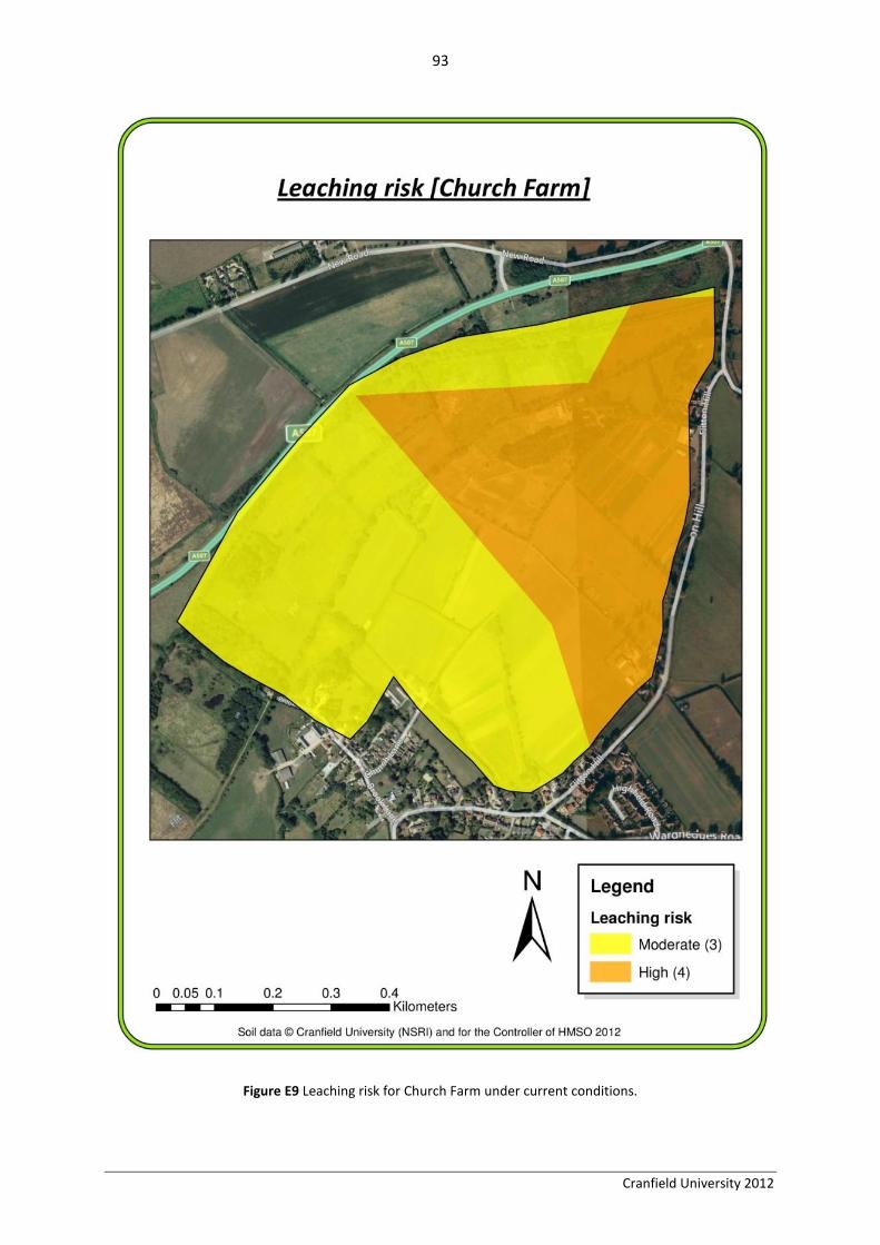
93
Cranfield University 2012
Figure E9 Leaching risk for Church Farm under current conditions.

94
Cranfield University 2012
Figure E10 Overland flow risk for Church Farm under current conditions.

95
Cranfield University 2012
Compared to the arable area, the grassland areas show a lower risk level for both leaching and
overland flow. Arable land on loam soils over red sandstone and on seasonally wet deep clay soils
were predicted to have a high risk of pollution from leaching, compared to a moderate level of risk
for the pasture. For overland flow risk, seasonally wet deep clay within arable land was predicted to
be of high risk. All other combinations of soil type and land use had a low risk.
Discussion
As cited in the literature, Brady and Weil (2010) indicate that leaching is influenced by the size and
configuration of soil pores. Preferential flow increases the possibility of polluting groundwater (e.g.
clay has worse proprieties for water flow than sand. But if it is dried and cracks appear in it, they
could become a quicker and easier way for the water to flow, and consequently pollutants) (Brady
and Weil 2010). In general, sandy soils have high leaching potential for pollutants, silty soils have
medium potential and clayey ones have a low potential (unless cracked) (Brady and Weil 2010).
These facts can be observed in the results table for leaching risk. The low risk of pollution due to
leaching from pasture, compared to arable production, is linked to the absence of pesticide risk.
Recommendations
At least some of the operation at Church Farm is currently managed in an organic way. As a certified
organic producer, the farm is expected to comply with the Compendium of UK Organic Standards
(2004) and any extra requirements of the chosen Certification Body (DEFRA, 2009). As an organic
farm, the farm could be eligible for the Organic Entry Level Stewardship (OELS) Scheme (Natural
England, 2010b). There are OELS measures (Table E11) which can improve water quality, by
reducing the source of nitrates and pesticides.

96
Cranfield University 2012
Table E11 ELS/OELS management recommendations to prevent pollution at source and therefore improve water quality (Natural England, 2010a). Note that ↓ means
reduced impact in the relative regulating ecosystem service; ↓ is reduction in impact, ↓↓ is significant reduction in impact, ↓↓↓ is dramatically high reduction in
impact.
OELS [ELS] code OES stipulation Location
Impact on runoff (nitrate,
phosphate, pesticide and
sediment pathway)
Impact on soil erosion (nitrate, phosphate and
pesticide pathway)
Recommendation
OU1 Organic Management Whole field ↓↓ ↓↓
No application of fertilisers, pesticides or any
herbicides. Application of nitrogen sourced from
animal manures limited to an average of 170kg/ha/yr
(not exceeding 250kg/ha on any one field parcel)
SPECIFIC TO PROTECTING SOIL AND WATER (EJ)
OJ2/
OJ10 [EJ2/EJ10]
Management of maize crops
Whole field ↓ ↓ Same management as ELS
OJ5 [EJ5]
Infield grass areas to prevent erosion and
runoff Within field ↓↓ ↓
Same management as ELS except that injurious weeds or invasive non-native species are to be controlled by cultivation before establishment, by cutting in the first year and by selective trimming or manual removal thereafter.
OJ5 [EJ5] Field margin grass areas (buffer strips)
Edge of field ↓↓ ↓
Same management as ELS except that injurious weeds or invasive non-native species are to be controlled by cultivation before establishment, by cutting in the first year and by selective trimming or manual removal thereafter.
OJ9 [EJ9] 12m buffer strips for Close to ↓↓ ↓ Same management as ELS except that injurious

97
Cranfield University 2012
watercourses on rotational land.
watercourses weeds or invasive non-native species are to be controlled by cultivation before establishment, by cutting in the first year and by selective trimming or manual removal thereafter.
OJ11 [EJ11]
Maintenance of
watercourse fencing
Edge of field/close to watercourses
↓ ↓ Same management as ELS
OJ13 [EJ13]
Winter cover crops Whole field ↓ ↓
Same management as ELS
MULTI-FUNCTIONAL: CONTRIBUTES TO PROTECTION OF SOIL AND WATER
OB1/OB2/OB3 [EB1/EB2/EB3]
Field boundary feature: Hedgerow
management Edge of field ↓ ↓
Same management as ELS
OB6 [EB6] Field boundary feature:
Ditch management Edge of field ↓ n/a
Same management as ELS
OC4 [EC4] Trees and Woodland:
Management of woodland edges
Edge of woodland at
edge or within field
↓↓ n/a
Same management as ELS except only apply herbicides to spot treat or weed-wipe for the control of injurious weeds or invasive non-native species and do not apply fertilisers or manures.
OC24 [EC24]
Tree and woodland: Hedgerow tree buffer
strips on rotational and organic grassland
Within field/edge of
field ↓↓ n/a
Same management as ELS except only apply herbicides to spot treat or weed-wipe for the control of injurious weeds or invasive non-native species.
OE1/OE2/OE3
OE4/OE5/OE6
[EE1/EE2/EE3/
EE5/EE6/EE6]
Buffer strips (managed as low intensity
grassland): 2-6m buffer strips on rotational
land and organic grassland.
Within field/edge of
field ↓↓ n/a
Same management as ELS except that injurious weeds or invasive non-native species are to be controlled by cultivation before establishment, by cutting in the first year and by selective trimming or manual removal thereafter.

98
Cranfield University 2012
OE10 [EE10] 6m buffering on
organic grassland next to a watercourse
Within field/edge of
field ↓ ↓ Same management as ELS
OF1/OL1 [EF1/EL1]
Management of arable, rotational and
grassland: Management of field
corners
Edge of field ↓↓ ↓
Same management as ELS except that injurious weeds or invasive non-native species are to be controlled by cultivation before establishment, by cutting in the first year and by selective trimming or manual removal thereafter.
OF6 [EF6]
Management of arable and rotational land:
Overwintered stubble and extended
overwintered stubble
Whole Field ↓ ↓ Same management as ELS.
OL2 [EL2]
Grassland: Permanent grassland with low
inputs of fertilisers and sprays
Whole field ↓↓ ↓↓
Apply up to 12.5tonnes/ha per year of farm yard manure, but only where grassland is regularly cut. Apply during growing season and only when field dry enough to prevent soil compaction. No other type of fertiliser or manures to be applied. If current manure and fertiliser use is less than this, do not increase applications. Injurious weeds or invasive non-native species are to be controlled by cultivation before establishment, by cutting in the first year and by selective trimming or manual removal thereafter.
OL3 [EL3]
Grassland: Permanent grassland with very low inputs of fertilisers and
sprays
Whole field ↓↓↓ ↓↓
Same management as ELS except that injurious weeds or invasive non-native species are to be controlled by cultivation before establishment, by cutting in the first year and by selective trimming or manual removal thereafter.

99
Cranfield University 2012
E3: Jubilee Woodland: Future BAP scenario
E3.1: Introduction
Biggleswade Woodland is one of the woodland tree plantation projects that is participating in the
Jubilee woodland project by the Woodland Trust. The project aims to plant 6 million trees in the UK
(The Woodland Trust 2012). The 8 ha area is located on the outskirts of Biggleswade and is located
near a stream that discharges into the River Ivel (Figure E11a). The area is generally flat with an
average slope of 1.30°; the surrounding area is also relatively flat. Previously, the land was used as
pasture, and the surrounding area is mostly arable land. The site has loamy/clayey soil with slightly
impeded drainage (NSRI 2008a, b, c) and is highly fertile (NSRI 2008a, b, c) (Figure E11b).
Figure E11a Location of study site at Jubilee Woodland, Biggleswade.

100
Cranfield University 2012
Figure E11b The Jubilee Woodland showing land use and soil type (NSRI 2008a, b, and c, 2009)

101
Cranfield University 2012
E3.2: Soil organic carbon
Methodology
It was assumed for the purposes of the case study that the entire area will be converted to
woodland vegetation land use, and the mean value for woodland vegetation (rather than any sub-
class) was used for the conversion. This was because it had values for each soil type, with no gaps. A
similar method was used as with the scenario, whereby new SOC density values were assigned for
each soil type, based on the mean value for that soil type under the future land use, i.e. woodland
vegetation. Then the difference between the current and future SOC density was calculated to
produce a map of SOC change (t ha-1).
Results

102
Cranfield University 2012
Figure E12 Predicted changes in soil organic carbon following the afforestation of the proposed site of the
Jubilee Woodland near Biggleswade, shown overlaid on a basemap from Bing Maps Hybrid, available in ESRI
ArcGIS 10.0.
Table E12 Initial and predicted SOC densities, and the difference between the two, for different soil types at
the Jubilee Woodland site near Biggleswade.
Soil type Initial SOC density (t
ha-1) Predicted SOC density (t ha-1)
SOC gain (t ha-1)
SOC gain (%)
Deep clay 186 235 49 26
Deep loam 127 180 53 42
Deep loam over gravel
94 142 47 50
Table E13 Initial and predicted SOC in tons, and the difference between the two, for the different soil types
and in total at the Jubilee Woodland site near Biggleswade.
Soil type Area (ha)
Initial SOC (tons)
Predicted SOC (tons)
SOC gain (tons)
Deep clay 12 2202 2783 581
Deep loam 5 650 921 271
Deep loam over gravel 4 375 563 187
Total 21 3228 4267 1040
It is clear from the map and tables above that it is predicted there will be significant gains in SOC
following afforestation of the site of the Jubilee Woodland. All three soil types will gain roughly the
same amount of SOC in terms of tons per hectare, with roughly 50 t ha-1each. Overall, the
afforestation of the site will cause an increase in SOC of 1040 tons, increasing the amount of SOC on
the site from an initial 3228 tons to 4267 tons; this is a staggering increase of nearly a third.
Discussion
It has generally been found in the literature and in this study that a conversion of arable land to
woodland vegetation causes an increase in SOC. All soils present at the Jubilee Woodland site gain
roughly the same amount of SOC in terms of t ha-1. Therefore, afforestation of arable land is highly
beneficial in terms of SOC gained.

103
Cranfield University 2012
Part E3.3: Runoff and soil erosion
D3.3.1Erosion
Methodology
Due to the presence of three soil types in the field, the K factor takes 3 different values (0.087,
0.118, and 0.123). LS varies across the field from 1 to 189 with a average of 30.3 and a standard
deviation of 23.1. The C factor changes with the land use from 0.025 for pasture to 0.001 for the
future forest. P and R remain constant equal to 1 and 66.14 respectively. Erosion rate was calculated
within the field with a 10m resolution.
Results
Figure E13 represents annual soil loss within the field. The land use change allows to cut soil loss by
96% from 44.5 to 1.8 ton/year in the 7.91 ha field. This corresponds to a soil loss reduction from 3.56
to 0.14 t/year.
Figure E13 Predicted erosion rate under forest land cover for Biggleswade Jubilee Woodland.

104
Cranfield University 2012
Discussion
As BAP scenario, pasture scenario and woodland scenario, this case study shows that the most
efficient land use to reduce erosion is the woodland. Therefore, it should be encourage in areas
where erosion reduction is a priority. Moreover, well designed forests close to urban areas have a
great cultural, ecological and aesthetic value (Forest of Marston Vale 2000).
Runoff
Methodology
Runoff generation was assessed under the Curve Number method. The site has three different
hydrologic soil types. Table E14 summarises the characteristics of the three patches at stake
assuming fair soil condition. Average previous wetness was assumed (condition II in the Curve
Number hand book).
Table E14 Soil characteristics of future woodland in Biggleswade.
Patch_ID Area (ha)
Hydrologic Soil Group
Current CN (pasture)
Future CN (forest)
1 1.58 A 58 35
2 1.93 C 82 72
3 4.56 D 86 79
Results
Applying the formulas of the SCS method (section 3), it was found that the land use change allows a
37% decrease in runoff. Detailed numbers are given in table E15.
Table E15 Infiltration improvement for Biggleswade forest creation for 2 simulated storm events
Storm event Runoff pasture (m3) Runoff forest (m
3)
Runoff reduction (%)
Infiltration improvement (%)
Worst in 10 years* 932 583 37 13.9
Worst in 100 years** 1780 1120 37 21.5
*42.6mm per day, which given the area of the patch corresponds to a catch of 3440m3
**59.7mm per day, which given the area of the patch corresponds to a catch of 4820m3
Discussion
This example illustrates how efficient forest is at controlling runoff on a variety of soil types. Indeed,
the land use change to forest implies a significant reduction of runoff, even when the previous use is
pasture whose behaviour against runoff is considered fairly good. Therefore, woodland land use
should be suggested in areas where runoff reduction is a priority.

105
Cranfield University 2012
E3.4: Water Quality
Methodology
Methodology used for analysis was the same than used for the rest of the case studies, mapping
variation of leaching and overland flow risks.
Results
Table E16 Initial and predicted leaching risk and the difference between the two for different combinations of
soil type in arable in Biggleswade Woodland.
Land Use Soil type
Arable
Mean Leaching Risk
BAP Scenario Risk
Risk variation
Deep clay 3 2 1
Deep loam 4 3 1
Deep loam over gravel 4 2 2
Table E17 Initial and predicted overland flow risk and the difference between the two for different
combinations of soil type in arable in Biggleswade Woodland.
Land Use Soil type
Arable
Mean Overland flow Risk
BAP Scenario Risk
Risk variation
Deep clay 3 2 1
Deep loam 3 1 2
Deep loam over gravel 2 1 1

106
Cranfield University 2012
Figure E14 Predicted leaching risk variation following the Jubilee Woodland project.

107
Cranfield University 2012
Figure E15 Predicted overland flow risk variation following the Jubilee Woodland project, shown overlaid on a
basemap from Bing Maps Hybrid, available in ESRI ArcGIS 10.0.

108
Cranfield University 2012
Table E16 show that deep loam and deep loam over gravel have a high leaching risk compared to
deep clay that has a moderate level. A land use conversion to woodland means a general
improvement for leaching risk in the whole area, much more noticeable in the case of loam over
gravel that enhances 2 levels, to a low risk.
A similar situation is observed for overland flow, but with different characteristics (figure E15 and
table E17). Deep clay and deep loam show a moderate risk, worse than the low risk showed by loam
over gravel. Conversion to woodland also means improvement for overland flow risk. In this case,
deep loam is the soil type with the greater improvement, 2 levels, compared to the improvement of
one level for deep clay and deep loam over gravel.
Discussion
As the current land use is the same for the whole area, differences in the risk of both leaching and
overland flow can be attributed to soil type.
Arable areas are characterised by the use of chemicals (pesticides and fertilizers) which means that
all the possible pollutants are present in the area.
The higher leaching risk for loam and loam over gravel can be justified by soil particles and soil pores
size, which are larger for loamy soils than for clayey soils (Brady and Weil 2010). This fact could also
justify the greater risk of overland flow for deep clay and deep loam due to clay particles smaller size
and loam intermediate size what which allows easily transportation within runoff.
A general improvement in both the risks of leaching and overland flow is observed when the BAP is
implemented at this site, converting the area into woodland. For both risks, change could be due to
the absence of chemicals in woodland management, and specifically for overland flow risk as a result
of the improvement of vegetation cover what reduces erosion and runoff velocity contributing to
infiltration.
Recommendations
The planned conversion of the area to woodland is beneficial with regards to water quality.