Centralized Modeling of the Communication Space for Spectral Awareness … · 2009-10-07 · Centralized Modeling of the Communication Space for Spectral Awareness in Cognitive Radio

Centralized Modeling of the Communication Space forSpectral Awareness in Cognitive Radio Networks

Jens P. Elsner, Christian Koerner and Friedrich K. JondralUniversitat Karlsruhe (TH), Germany, {elsner, koerner, fj}@int.uni-karlsruhe.de

The communication space is five dimensional: its degrees of freedom are frequency, timeand space. The use of the electromagnetic spectrum depends on these parameters. With fu-ture applications such as opportunistic overlay access or distributed spectrum monitoringin mind, it is important to estimate the state of the communication space on the basis ofincomplete or imprecise information. A promising approach are technology centric Cogni-tive Radio networks. In these networks, nodes cooperate to infer information on spectraloccupancy. This conceptual paper proposes a novel approach for centralized modelingof the communication space with emphasis on spatial dependencies through the use of aregression model. The modeling approach is verified with practical measurements.

I. Introduction

The five dimensional communication space is spannedby the dimensions frequency, time and space1. Theusage of the natural resource electromagnetic spec-trum varies with these parameters. Access to spec-trum is heavily regulated in all parts of the world. Tra-ditionally, the access rules governing spectrum usageare formulated in terms of frequency ranges, largelyignoring the two remaining degrees of freedom: timeand space. This historical approach to licensing haslead to inefficient use of spectrum. E.g., [2] reports anaverage load of 5.2 percent in the 3 - 3000 MHz range,leaving a lot of room for improvement.

To increase the efficiency in spectrum usage, trans-missions of an overlay system can take place in trans-mission opportunities or spectrum holes [3, 4]. Trans-mission opportunities are unused regions of the com-munication space spanned by time, frequency and lo-cation. The detection of spectrum holes has to be ac-curate to decrease the probability of interference withother systems. Due to the nature of measurements,identification of transmission opportunities is alwaysbased on incomplete and imprecise information. Con-ceptual challenges in radio networks such as the hid-den node and exposed node problem suggest the useof cooperative identification of transmission opportu-nies, i.e., information sharing between wireless termi-nals.

A centralized modeling approach is considered inthis paper: wireless terminals gather local information

1This work has been presented in part at the IEEE Workshopon Cognitive Radios, Las Vegas, USA, January 2008 [1]. It hasbeen expanded to include practical measurement and regulatoryconsiderations, a conceptual engine description and extended re-sults.

on their environment (e.g. spectrum usage, location)and forward this information to a centralized instance,termed network. The network uses this informationfrom distributed nodes to build an online model of thecommunication space state. This spectral awarenesscan then be used to optimize resource allocation.

The remainder of this paper is structured as fol-lows: after a brief conceptual introduction to spectralawareness and its applications in this Section, SectionII describes capabilities and requirements for spectralestimation in a Cognitive Radio (CR) terminal. Sec-tion III covers centralized modeling of the communi-cations space. Concluding remarks and a summary ofimportant research problems form Section IV.

I.A. Scenario

We consider a distribution of wireless nodes con-nected to a central instance. This central instance isreferred to as network. The scenario is depicted inFigure 1. All CR terminals are assumed to have anout-of-band connection to the network2. Furthermore,the network is aware of the position of each CR ter-minal. This location awareness is a precondition formodeling of spatial dependencies and currently underinvestigation by numerous researchers [4, 5].

During operation, the CR terminals report infor-mation relevant to the state of the communicationspace to the network. This relevant information isan estimate of the spectral environment and an esti-mate of the current CR terminal position, which thenetwork tracks. Based on the reported information,the network builds a model of the communication

2The nature of this feedback channel is not considered hereand is in fact a fundamental conceptual issue of CR networks [4].

62 Mobile Computing and Communications Review, Volume 13, Number 2

node A

node Bnode C

node D

network

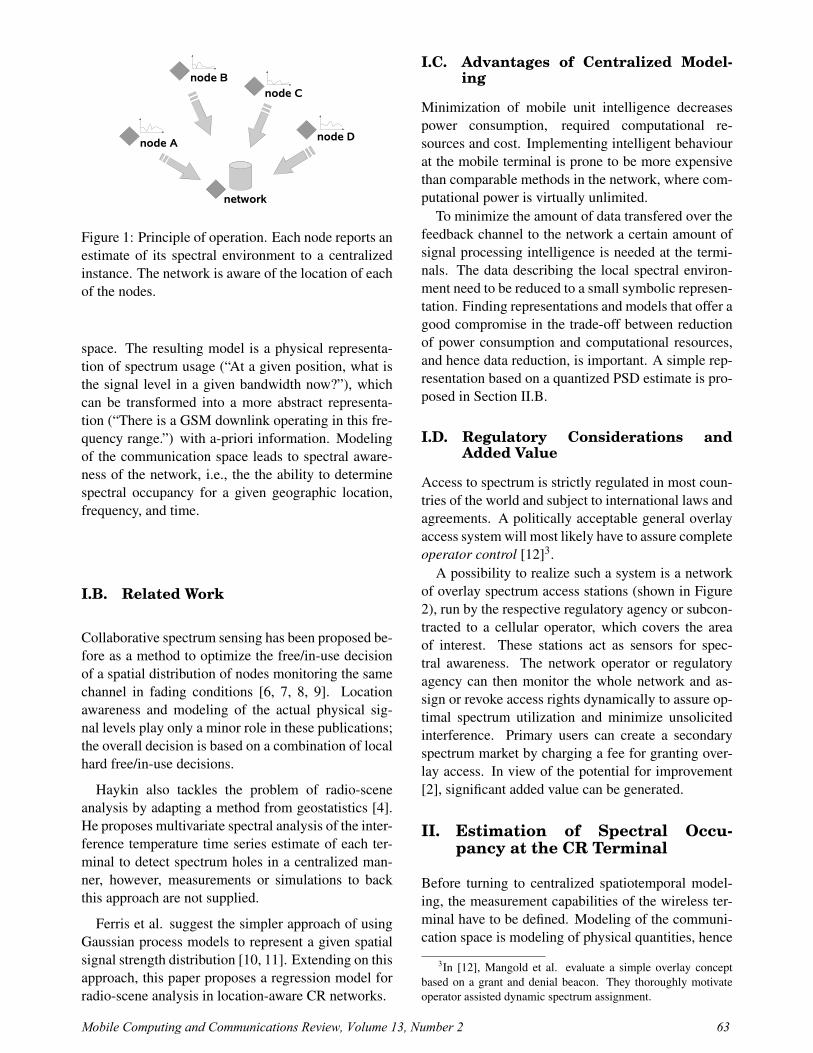
Figure 1: Principle of operation. Each node reports anestimate of its spectral environment to a centralizedinstance. The network is aware of the location of eachof the nodes.

space. The resulting model is a physical representa-tion of spectrum usage (“At a given position, what isthe signal level in a given bandwidth now?”), whichcan be transformed into a more abstract representa-tion (“There is a GSM downlink operating in this fre-quency range.”) with a-priori information. Modelingof the communication space leads to spectral aware-ness of the network, i.e., the the ability to determinespectral occupancy for a given geographic location,frequency, and time.

I.B. Related Work

Collaborative spectrum sensing has been proposed be-fore as a method to optimize the free/in-use decisionof a spatial distribution of nodes monitoring the samechannel in fading conditions [6, 7, 8, 9]. Locationawareness and modeling of the actual physical sig-nal levels play only a minor role in these publications;the overall decision is based on a combination of localhard free/in-use decisions.

Haykin also tackles the problem of radio-sceneanalysis by adapting a method from geostatistics [4].He proposes multivariate spectral analysis of the inter-ference temperature time series estimate of each ter-minal to detect spectrum holes in a centralized man-ner, however, measurements or simulations to backthis approach are not supplied.

Ferris et al. suggest the simpler approach of usingGaussian process models to represent a given spatialsignal strength distribution [10, 11]. Extending on thisapproach, this paper proposes a regression model forradio-scene analysis in location-aware CR networks.

I.C. Advantages of Centralized Model-ing

Minimization of mobile unit intelligence decreasespower consumption, required computational re-sources and cost. Implementing intelligent behaviourat the mobile terminal is prone to be more expensivethan comparable methods in the network, where com-putational power is virtually unlimited.

To minimize the amount of data transfered over thefeedback channel to the network a certain amount ofsignal processing intelligence is needed at the termi-nals. The data describing the local spectral environ-ment need to be reduced to a small symbolic represen-tation. Finding representations and models that offer agood compromise in the trade-off between reductionof power consumption and computational resources,and hence data reduction, is important. A simple rep-resentation based on a quantized PSD estimate is pro-posed in Section II.B.

I.D. Regulatory Considerations andAdded Value

Access to spectrum is strictly regulated in most coun-tries of the world and subject to international laws andagreements. A politically acceptable general overlayaccess system will most likely have to assure completeoperator control [12]3.

A possibility to realize such a system is a networkof overlay spectrum access stations (shown in Figure2), run by the respective regulatory agency or subcon-tracted to a cellular operator, which covers the areaof interest. These stations act as sensors for spec-tral awareness. The network operator or regulatoryagency can then monitor the whole network and as-sign or revoke access rights dynamically to assure op-timal spectrum utilization and minimize unsolicitedinterference. Primary users can create a secondaryspectrum market by charging a fee for granting over-lay access. In view of the potential for improvement[2], significant added value can be generated.

II. Estimation of Spectral Occu-pancy at the CR Terminal

Before turning to centralized spatiotemporal model-ing, the measurement capabilities of the wireless ter-minal have to be defined. Modeling of the communi-cation space is modeling of physical quantities, hence

3In [12], Mangold et al. evaluate a simple overlay conceptbased on a grant and denial beacon. They thoroughly motivateoperator assisted dynamic spectrum assignment.

Mobile Computing and Communications Review, Volume 13, Number 2 63

network

network

network

(a) Distributed centralized modeling in a overlay ac-cess network. A model is run for each area of in-terest. The spectrum access stations act as sensorsfor the spectral environment and collect informationfrom the CR terminals.

network

short term statistics, compress

channelize measurements

PSD estimate

terminal report

spatiotemporal modeling

(b) Principle steps from spectral estimation to cen-tralized model building. At the terminal, the PSDestimate is compressed (e.g. by channel segmenta-tion, quantizing) and then reported to the network.The network collects the measurements and aggre-gates them in discrete channels. Each channel isthen modeled separately.

Figure 2: Principle of operation

measurements of the CR terminal have to be made in-dependent of a specific wireless standard. This im-plies a three step process at the CR terminal shown inFigure 2.

In a first step, the CR terminal node measures asignal level, possibly making use of a-priori informa-tion (matched filtering, feature detection). In a secondstep, this information is aggregated, compressed andthen, in a third step, forwarded to the network. Thenetwork then uses this data to model the communica-tion space occupancy.

The most general measurement step is spectral es-timation, an energy based detection strategy.

II.A. Spectral Estimation

Spectral estimation, also known as spectral analysisor spectrum sensing in a CR context, is the simpleststandard independent detection strategy. The mea-surement capabilities of a CR terminal with spectrumestimation comprise three basic steps:

1. Appropriate spectral estimation with respect totime and frequency resolution,

2. (optional) channel segmentation,

3. spectrum estimate compression (e.g. throughquantization) and reporting.

Maximum Hold

For inherently instationary signals such as communi-cation signals, spectral estimation algorithms can un-derestimate the maximum signal level in a given fre-quency range. E.g., if we choose to average peri-odograms over the duration of a whole GSM time di-vision multiple access (TDMA) frame with only oneactive burst (cf. Figure 3 and 5), the resulting PSD es-timate significantly underestimates the maximum re-ceived power. A comparison with a peak-hold esti-mate serves as an indicator that the averaging dura-tion is too long: the estimated variance is higher thanthe expected variance for a given algorithm. This factcan be exploited to adapt spectral resolution, temporalresolution and window length to the data to get a moreaccurate maximum power estimate.

Time - Frequency Resolution

Spectral estimation methods have an inherent trade-off between time resolution and frequency resolution.Choosing a long averaging duration results in goodfrequency resolution but poor localization of frequen-cies in time. A short duration on the other hand givespoor frequency resolution but good localization of fre-quencies. This is illustrated in Figure 3, a snapshotof a GSM1800 downlink band. With high tempo-ral resolution the burst structure and power control isclearly visible but the channel bandwidth is overes-


−2 −1 0 1 2

5

10

15

20

25

30

frequency (MHz)

time

(ms)

dB

−15

−10

−5

0

5

10

15

(a) High temporal resolution

−2 −1 0 1 2

5

10

15

20

25

30

frequency (MHz)

time

(ms)

dB

−15

−10

−5

0

5

10

15

20

25

30

(b) High frequency resolution

Figure 3: Illustration of the influence of the time and frequency resolution choice. The time-frequency planeshown has a center frequency within the GSM 1800 band at 4 MHz bandwidth. Both planes were computed from131072 samples based on the Welch method with a Hamming window, yielding a frequency-time resolution of64× 2048 bins in Figure 3(a) and 2048× 64 bins in Figure 3(b). Note the frequency leakage in Figure 3(a).

timated due to leakage. Choosing a long averagingduration and hence a high frequency resolution leadsto a good estimate of the channel bandwidth while theburst structure is blurred. Furthermore, both time andfrequency resolution can be traded against accuracy ofthe estimate.

II.B. Data Representation and Report-ing

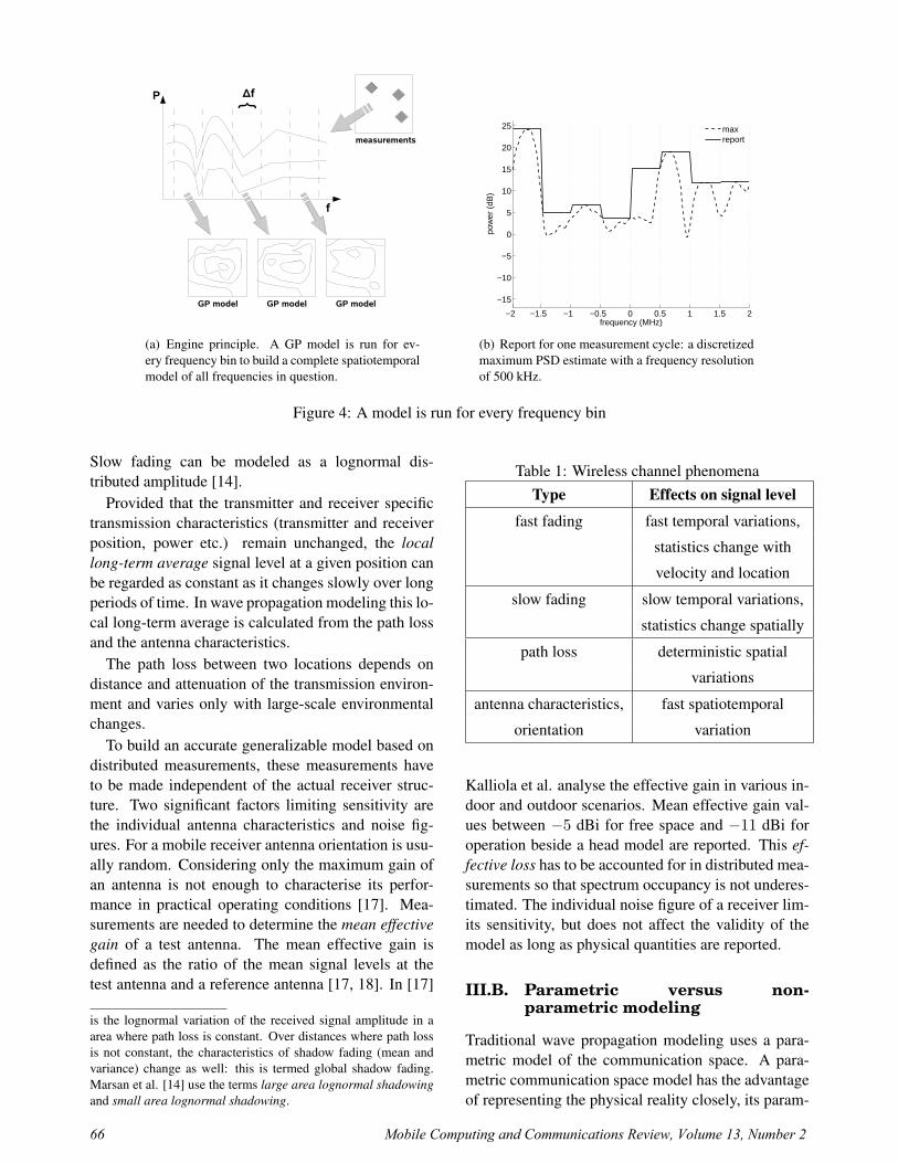
The output of the spectral estimation stage is a quan-tized PSD, essentially a description of channels andsignal levels. Figure 4(b) shows such an estimate. Op-tional channel segmentation can increase the accuracyof the PSD estimate, as quantization for data compres-sion prior to reporting to the network can then be car-ried out more exactly. With the prior knowledge of thematched filters, the node can precisely report a singlepower estimate per channel and time slot.

III. Centralized Modeling of theCommunication Space

The state of the communication space is the spa-tiotemporal distribution of signal levels in units ofWatt per Hertz: loosely speaking, a spatial general-ization of the power spectral density. An equivalentmetric, interference temperature, has been proposedby the FCC Spectrum Policy Task Force [13]. It is thechoice of the designer of the CR terminal whether touse the spectrum estimation/energy detection, equiva-lent to the interference temperature metric, or methods

with increased sensitivity incorporating prior knowl-edge such as matched filtering. The following spa-tiotemporal model has to be independent of the powermeasurement method chosen.

III.A. Physical Properties of the Wire-less Communication Channel

The physics of wave propagation, i.e., phenomenasuch as attenuation, refraction and reflection, lead tospatial and temporal dependencies of the electromag-netic field strength.

For any given center frequency and receiver lo-cation, two stochastic phenomena dominate the spa-tiotemporal characteristics of the receiver signal level,i.e., the absolute values of the complex voltages at thereceiver: fast fading and slow fading, also known asshadow fading. A third factor, long-distance variationof the signal level, can be regarded as deterministicand is described by the path loss between transmitterand receiver.

Fast fading is the location-independent fast varia-tion of the signal amplitude and phase, attributed tovarying multi-path propagation due to moving scat-teres and receiver movements in the order of a wave-length [14]. The influence of fast fading on the signalis usually modeled by a Rayleigh or Rice amplitudedistribution [15].

Slow fading is the variation of the local mean powerover distances in the order of tens of wavelengths4.

4Salo et al. [16] distinguish between local shadow fading andglobal shadow fading. According to Salo, local shadow fading


Δf

}

f

P

GP model

measurements

GP model GP model

(a) Engine principle. A GP model is run for ev-ery frequency bin to build a complete spatiotemporalmodel of all frequencies in question.

−2 −1.5 −1 −0.5 0 0.5 1 1.5 2

−15

−10

−5

0

5

10

15

20

25

frequency (MHz)

pow

er (

dB)

maxreport

(b) Report for one measurement cycle: a discretizedmaximum PSD estimate with a frequency resolutionof 500 kHz.

Figure 4: A model is run for every frequency bin

Slow fading can be modeled as a lognormal dis-tributed amplitude [14].

Provided that the transmitter and receiver specifictransmission characteristics (transmitter and receiverposition, power etc.) remain unchanged, the locallong-term average signal level at a given position canbe regarded as constant as it changes slowly over longperiods of time. In wave propagation modeling this lo-cal long-term average is calculated from the path lossand the antenna characteristics.

The path loss between two locations depends ondistance and attenuation of the transmission environ-ment and varies only with large-scale environmentalchanges.

To build an accurate generalizable model based ondistributed measurements, these measurements haveto be made independent of the actual receiver struc-ture. Two significant factors limiting sensitivity arethe individual antenna characteristics and noise fig-ures. For a mobile receiver antenna orientation is usu-ally random. Considering only the maximum gain ofan antenna is not enough to characterise its perfor-mance in practical operating conditions [17]. Mea-surements are needed to determine the mean effectivegain of a test antenna. The mean effective gain isdefined as the ratio of the mean signal levels at thetest antenna and a reference antenna [17, 18]. In [17]

is the lognormal variation of the received signal amplitude in aarea where path loss is constant. Over distances where path lossis not constant, the characteristics of shadow fading (mean andvariance) change as well: this is termed global shadow fading.Marsan et al. [14] use the terms large area lognormal shadowingand small area lognormal shadowing.

Table 1: Wireless channel phenomenaType Effects on signal level

fast fading fast temporal variations,

statistics change with

velocity and location

slow fading slow temporal variations,

statistics change spatially

path loss deterministic spatial

variations

antenna characteristics, fast spatiotemporal

orientation variation

Kalliola et al. analyse the effective gain in various in-door and outdoor scenarios. Mean effective gain val-ues between −5 dBi for free space and −11 dBi foroperation beside a head model are reported. This ef-fective loss has to be accounted for in distributed mea-surements so that spectrum occupancy is not underes-timated. The individual noise figure of a receiver lim-its sensitivity, but does not affect the validity of themodel as long as physical quantities are reported.

III.B. Parametric versus non-parametric modeling

Traditional wave propagation modeling uses a para-metric model of the communication space. A para-metric communication space model has the advantageof representing the physical reality closely, its param-


eters are number, position and power of transmitters,antenna characteristics and wave propagation environ-ment. If these parameters are known, techniques fromwave propagation modeling can be applied to makecoverage predictions. Standard approaches includesimple path loss calculations, simplified diffraction-based methods, ray tracing and field theoretic calcu-lations [15]. The type of model used in a given ap-plication depends heavily on frequency, desired accu-racy and terrain at hand. Sophisticated models useterrain information for relatively precise predictions.Unfortunately, even with these models the standarddeviation of the prediction error is in the order of10 dB [19] as the physical reality contains too manyunknown factors (e.g. metal contents of buildings,non-stationary environmental influences such as traf-fic and weather conditions) to be precise. In practice,predictions are verified and fine-tuned with measure-ments [19]. This shows that even very complex mod-els represent the physical environment inadequately.A parametric communication space model would haveto estimate the right combination of number of trans-mitters, antennae characteristics etc. from an infi-nite number of possibilities. Without a-priori informa-tion this is infeasible - a communication space modelrelying on measurements only is bound to be non-parametric5.

III.C. Choosing effects to model

The spectral estimation step proposed in Section II re-sults in a PSD estimate. The PSD does not includephase information. Accordingly, we are only inter-ested in modeling receiver signal levels, i.e., the abso-lute values of the complex voltages at the receiver an-tenna, and not the complete channel impulse response.

Table 1 shows the different wireless channel phe-nomena. The communication space model has to pro-vide means to capture the most significant effects. Tosummarize: for a fixed location, there are variations inthe signal level over time due to fading and transmitteractivity. For a fixed moment in time, there are spatialvariations in the signal level due to path loss.

The model should capture only spatiotemporal de-pendencies directly related to spectrum occupancy.Hence, we are interested in modeling deterministicspatial variations due to path loss, spatial statistical

5Even if a direct parametric modeling approach seems infeasi-ble, it is possible to infer information about locations and numberof transmitters and transmission characteristics in a second step.A parametric representation of the cause of the communicationspace state can be built on top of the non-parametric effect model:this of interest when monitoring unsolicited interference.

variations due to slow fading on top of path loss, andtransmitter activity. Fast fading is eliminated at theCR terminal during measurement by averaging.

The concrete local long-term average of the receivepower PR(xR)6 at the receiver location is calculatedwith the radiated equivalent isotropic radiated powerPT(xT), transmitter antenna gain GT, receiver antennagain GR and path loss D(xT,xR), depending on bothreceiver and transmitter location:

PR(xR) = PT(xT) + GT + GR (1)

−D(xT,xR) [dB]

The measured power at the receivers is equivalent to

PM(xR) = PR(xR)−GR + DSF [dB], (2)

where PR(xR) − GR is the variable to be modeled inthis work and DSF denotes slow fading and is equiva-lent to the measurement noise.

To account for different antenna characteristics, itis assumed that all measurements are normalized ac-cording to the mean effective gain of the receiver an-tenna.

The goal of the model is to capture the effects, notthe cause of spatial spectrum occupation. Separatingthe effects from the cause allows for non-parametricmodeling.

Spatial Dependencies

Measurements are only available for distinct loca-tions. The model should make resonable predic-tions for locations without measurements, interpolat-ing from available data. A good interpolation methodshould also provide a measure of reliability. Themodel should capture deterministic spatial variationsin a path loss component and spatial statistical varia-tions caused by slow fading.

Gaussian process regression, also known as krig-ing7, is a modeling method from geostatistics. Us-ing Gaussian processes (GPs) as a statistical non-parametric model offers an elegant way to representlocation-dependent spectrum usage.

A key question to be answered is that of spatial cor-relation between measurements, i.e., the question ofrelevancy of observations in one location to neighbor-ing locations. Spatial correlation of signal strengthmeasurements has been studied extensively in litera-ture, c.f. [21, 22] and references therein. These stud-ies aim at describing the stochastic properties of sig-nal strength distribution to develop suitable wireless

6Bold script denotes a collection of variables or a vector.7Named after South African mining engineer D. G. Krige [20].


channel simulations for different propagation environ-ments. Extending this idea, it is possible with georef-erenced statistics, i.e., location aware CR terminals, toembed measurements into a stochastic framework.

III.D. Regression with Gaussian Pro-cesses

A Gaussian process (GP) is a set of random variablesdenoted by f(xi), any finite number of which have ajointly Gaussian distribution8 [20].

The value of the underlying latent function at a lo-cation xi is represented by the GP f(xi). A GP isdefined by its mean

m(x) = E{f(x)} (3)

and covariance function cov(f(xp), f(xq)) =k(xp,xq),

k(xp,xq) = E{(f(xp)−m(xp))(f(xq)−m(xq))}.(4)

Without loss of generality, the mean function can beassumed to be zero. If the covariance function is prop-erly defined9, a GP can be used as a non-parametricmodel for machine learning: an observation (yi,xi)is thought to be related to the random variable f(xi)modeling a latent function. With a signal model anda given set of n observations D = {(yi,xi)|i =1, ..., n}, the model calculates the posterior distribu-tion of the GP at a test point.

Predictions with Noisy Observations

The signal model is defined as

y = f(x) + ε, (5)

where ε is additive independent Gaussian noise withvariance σ2

n. Taking into account the additive Gaus-sian noise, the covariance between the observationscan be written as

cov(yp, yq) = k(xp,xq) + σ2nδpq , (6)

where δpq denotes the Kronecker delta which is oneiff p = q and zero otherwise.

The n × n covariance matrix Ky of a set of noisyobservations is then

Kyp,q = cov(yp, yq) . (7)

8We follow the function-space view of Rasmussen andWilliams [20].

9The resulting covariance matrix needs to be invertible [20].

Let k(x∗) be the n× 1 vector of covariances betweenthe training points, i.e., locations at which observa-tions were obtained, and an arbitrary test point x∗:

k(x∗) = [k(x1,x∗), ..., k(xm,x∗)]T . (8)

The conditional mean with zero prior mean m(x) andvariance at the test point are then calculated as [20]

µx∗ = m∗(x∗) = k(x∗)T K−1y y (9)

and

σ2x∗ = k∗(x∗,x∗) = k(x∗,x∗)− kT

∗ K−1y k∗. (10)

The regression model is given by (9) and (10). Tomake predictions using the model an appropriate co-variance function has to be specified. This covariancefunction is application specific. The principal shapeof the covariance function is chosen based on a-prioriknowledge. The shape still has remaining degrees offreedom, the so-called hyperparameters. These hyper-parameters are estimated from the measurement dataas a whole. For a spatial signal strength distributionmodel, yi is a measurement at a location xi. Tak-ing the stochastic properties of shadow fading intoaccount, an exponential covariance function is an ap-propriate choice for modeling two dimensional spa-tial data as shown by Giancristofaro and Gudmundson[22, 23]:

k(xi,xj) = σ2f exp

((xj − xi)Σ(xj − xi)T

)+σ2

nδpq

with Σ = diag(1/l2x, 1/l2y) . (11)

A stochastic process with this covariance function isstationary in space, as it is only a function of the dis-tance of two locations |xj − xi|. The squared expo-nential covariance has different characteristic lengthslx and ly, allowing different correlation properties onthe x and y scale. σf is the GP model standard devia-tion, σn is the standard deviation of the measurementnoise. All hyperparameters Θ = [lx, ly, σ

2f , σ2

n]T

need to be estimated from the data. The maximumlikelihood estimate is given by maximizing the like-lihood log p(y|D,Θ) or equivalently by minimizingthe objective function

f = log |Ky|+ yT K−1y y, (12)

where y is the vector of all observations. This opti-mization problem is efficiently solvable by conjugategradient descent [20].


Interpretation of Model Noise and Exem-plary Measurements

Figure 6 shows the result of GP regression for a chan-nel of the GSM900 band in contour plots10. The datais displayed for a varying number of measurements,made in the GSM900 bands and georeferenced withGPS accuracy. Areas in which the estimated cumula-tive model and noise standard deviation uncertaintyexceeds 6 dB are not plotted. In these areas, onlyfew measurements were made and hence the predic-tion is uncertain. As slow fading is lognormal dis-tributed, the GP model works on logarithmic measure-ment data. The prior mean function is assumed tobe zero, m(x) = 0; the measurement data are cen-tered to account for this assumption. σ2

n describesthe model noise and the variance of lognormal fad-ing. The location-independent fast fades are averagedout during the spectrum estimation and reporting step.

III.E. Extension to Temporal Dependen-cies

The GP model for spatial dependencies can easily begeneralized to include temporal dependencies. Onehas to differentiate between long term dependencies,which are covered by the model, and short term de-pendencies of the communication space which are notincluded. This has a very practical reason: short termdependencies cannot be modeled in a centralized man-ner as this information is lost during the sporadic re-porting stage. Furthermore, the model describes onlythe state of the communication space over, e.g., thelast few minutes. This state can be regarded as current,but it does provide information about future spectrumusage. Obviously then, short term communicationspace changes have to be dealt with at the terminal.

The centralized model has a temporal resolution ap-propriate to model longer term dependencies. Withrespect to overlay system use, this approach can beused to opportunistically reuse completely unused fre-quency ranges, which tend to stay free in certain areasfor longer periods of time.

Long term dependencies

The GP model can be generalized to include longterm dependencies by temporal windowing of mea-surement data. The underlying assumption, in anal-ogy to spectral estimation, is that the latent functionmodeled by GP regression can be treated as stationaryin the window duration.

10A verification of the model and further details can be foundin [1]

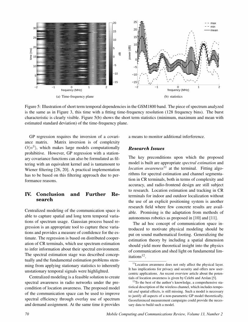
If only limited measurements are available, the sta-tionarity requirements can be relaxed if the wirelessterminals report only the maximum of all PSD es-timates to the network. Then, only the maximumsignal level for each channel has to be stationarity.This eliminates the influence of sporadic waveformsand separates long-term from short-term dependen-cies. An example is shown in Figure 5(b).

Short term dependencies

Short term dependencies are communication spacechanges not covered by the proposed GP model. Shortterm dependencies are, for example, the TDMA burststructure in a GSM system as shown in Figure 5(a) orthe periodic bursty nature of a RADAR sweep.

In an overlay context, modeling to exploit thesesmall scale transmission opportunities has to be donedirectly at the terminal. Several approaches have beenproposed in literature, e.g., Mangold et al. [24] sug-gest a histogram based approach, now part of the pro-posed IEEE 802.11k amendment [25].

If only long-term dependencies are modeled, it isnot guaranteed that, due to the processing delay ofthe network, a frequency resource assigned for trans-mission by the network, is indeed available. An over-lay terminal has to perform channel sensing regularlyto detect previously inactive primary system transmit-ters. If an active primary transmission is detected, ithas to back-off and report to the network.

III.F. Model Engine Concept

The spatial spectrum map, if available for differentfrequency ranges, can be used to identify transmis-sion opportunities in frequency and space, i.e, unusedfrequency ranges or areas in which the signal level isbelow a threshold.

A complete model of the communication space canbe constructed by running several regression modelsfor different frequency ranges. The spatial resolutionis not discretized a-priori but results from the definedtest point grid. The frequency resolution is chosensmaller than the smallest channel bandwidth of in-terest. The time resolution is a compromise betweennumber of measurements available and stationarity re-quirements.

For each frequency bin, a GP model is run, yield-ing a complete representation of the communicationspace. Figure 2 and Figure 4 illustrate the proposedconcept. The estimation of hyperparameters can bebased on the fact that the large scale environment isstationary and averaged over a long period of time.


−2 −1 0 1 2

5

10

15

20

25

30

frequency (MHz)

time

(ms)

dB

−15

−10

−5

0

5

10

15

20

(a) Time-frequency plane

−2 −1 0 1 2

−15

−10

−5

0

5

10

15

20

25

frequency (MHz)

pow

er (

dB)

maxminmean

(b) statistics

Figure 5: Illustration of short term temporal dependencies in the GSM1800 band. The piece of spectrum analyzedis the same as in Figure 3, this time with a fitting time-frequency resolution (128 frequency bins). The burstcharacteristic is clearly visible. Figure 5(b) shows the short term statistics (minimum, maximum and mean withestimated standard deviation) of the time-frequency plane.

GP regression requires the inversion of a covari-ance matrix. Matrix inversion is of complexityO(n3), which makes large models computationallyprohibitive. However, GP regression with a station-ary covariance functions can also be formulated as fil-tering with an equivalent kernel and is tantamount toWiener filtering [26, 20]. A practical implementationhas to be based on this filtering approach due to per-formance reasons.

IV. Conclusion and Further Re-search

Centralized modeling of the communication space isable to capture spatial and long term temporal varia-tions of spectrum usage. Gaussian process based re-gression is an appropriate tool to capture these varia-tions and provides a measure of confidence for the es-timate. The regression is based on distributed cooper-ation of CR terminals, which use spectrum estimationto infer information about their spectral environment.The spectral estimation stage was described concep-tually and the fundamental estimation problems stem-ming from applying stationary statistics to inherentlyunstationary temporal signals were highlighted.

Centralized modeling is a feasible solution to createspectral awareness in radio networks under the pre-condition of location awareness. The proposed modelof the communication space can be used to improvespectral efficiency through overlay use of spectrumand demand assignment. At the same time it provides

a means to monitor additional inferference.

Research Issues

The key preconditions upon which the proposedmodel is built are appropriate spectral estimation andlocation awareness11 at the terminal. Fitting algo-rithms for spectral estimation and channel segmenta-tion in CR terminals, both in terms of complexity andaccuracy, and radio-frontend design are still subjectto research. Location estimation and tracking in CRterminals for indoor and outdoor localization withoutthe use of an explicit positioning system is anotherresearch field where few concrete results are avail-able. Promising is the adaptation from methods ofautonomous robotics as proposed in [10] and [11].

The ad hoc concept of communication space in-troduced to motivate physical modeling should beput on sound mathematical footing. Generalizing theestimation theory by including a spatial dimensionshould yield more theoretical insight into the physicsof communication and shed light on fundamental lim-itations12.

11Location awareness does not only affect the physical layer.It has implications for privacy and security and offers new user-centric applications. An recent overview article about the poten-tials of location awareness is given by Celebi and Arslan [5].

12To the best of the author’s knowledge, a comprehensive sta-tistical description of the wireless channel, which includes tempo-ral and spatial effects, is still missing. Such a model is necessaryto justify all aspects of a non-parametric GP model theoretically.Georeferenced measurement campaigns could provide the neces-sary data to build such a model.


distance (m)

dist

ance

(m

)

−600 −400 −200 0 200 400 600

−400

−200

0

200

400

dBm

−90

−85

−80

−75

−70

−65

−60

−55

(a) 250 measurements

distance (m)

dist

ance

(m

)

−600 −400 −200 0 200 400 600

−400

−200

0

200

400

dBm

−90

−85

−80

−75

−70

−65

−60

−55

(b) 500 measurements

distance (m)

dist

ance

(m

)

−600 −400 −200 0 200 400 600

−400

−200

0

200

400

dBm

−90

−85

−80

−75

−70

−65

−60

−55

(c) 1000 measurements

distance (m)

dist

ance

(m

)

−600 −400 −200 0 200 400 600

−400

−200

0

200

400

dBm

−95

−90

−85

−80

−75

−70

−65

−60

−55

−50

(d) 2500 measurements

Figure 6: These contour plots show GP regression for models of varying complexity and 2σ < 12dBm, assuminglx = 40m, ly = 40m with lognormal noise of 3 dB standard deviation.


Last but not least the GP model itself has to be im-proved. Spatial non-stationary modeling is likely tobe more accurate in scenarios with different types ofenvironment [27]. Non-Gaussian noise models mighthelp to increase the robustness of the model againstoutliers [28]. Another important open question is therobustness against positional noise, neglected in thisstudy.

References

[1] J. P. Elsner, C. Korner, and F. K. Jondral, “Non-parameteric Modeling with Gaussian Processesfor Spatial Radio-Scene Analysis,” in Proceed-ings of the Consumer Communications and Net-working Conference, Las Vegas, USA, January2008.

[2] “Shared Spectrum Company,”http://www.sharedspectrum.com.

[3] F. K. Jondral, “Software Defined Radio - Basicsand Evolution to Cognitive Radio,” EURASIPJournal on Wireless Communications and Net-working, no. 3, pp. 275–283, 2005.

[4] S. Haykin, “Cognitive radio: brain-empoweredwireless communications,” IEEE Journal on Se-lected Areas in Communications, Feb. 2005.

[5] H. Celebi and H. Arslan, “Utilization of Lo-cation Information in Cognitive Wireless Net-works,” IEEE Wireless Communications, Aug.2007.

[6] E. Visotsky, S. Kuffer, and R. Peterson, “OnCollaborative Detection of TV Transmissions inSupport of Dynamic Spectrum Sharing,” Nov.2005.

[7] A. Ghasemi and E. S. Sousa, “CollaborativeSpectrum Sensing for Opportunistic Access inFading Environments,” Nov. 2005.

[8] S. M. Mishra, A. Sahai, and R. W. Brodersen,“Cooperative Sensing among Cognitive Radios,”in IEEE International Conference on Communi-cations, Jun. 2006.

[9] A. Ghasemi and E. S. Sousa, “AsymptoticPerformance of Collaborative Spectrum Sens-ing under Correlated Log-Normal Shadowing,”IEEE Communication Letters, Jan. 2007.

[10] B. Ferris, D. Hahnel, and D. Fox, “Gaussian Pro-cesses for Signal Strength-Based Location Es-timation,” in Proceedings of Robotics: Scienceand Systems, Philadelphia, USA, August 2006.

[11] B. Ferris, D. Fox, and N. Lawrence, “WiFi-SLAM Using Gaussian Process Latent VariableModels,” in Proceedings of the InternationalJoint Conferences on Artificial Intelligence, Hy-derabad, India, January 2007.

[12] S. Mangold, A. Jarosch, and C. Monney, “Op-erator Assisted Cognitive Radio and DynamicSpectrum Assignment with Dual Beacons - De-tailed Evaluation,” in First International Con-ference on Communication System Software andMiddleware, Jan. 2006.

[13] “Report of the Spectrum Efficiency WorkingGroup,” Federal Communications Commission- Spectrum Policy Task Force, Tech. Rep., Nov.2002, eT Docket no. 02-135.

[14] M. J. Marsan, G. C. Hess, and S. S. Gilbert,“Shadowing Variability in an Urban Land Mo-bile Environment at 900 MHz,” Electronics Let-ter, vol. 26, May 1990.

[15] N. Geng and W. Wiesbeck, Planungsmethodenfur die Mobilkommunikation, Funknetzplanungunter realen physikalischen Ausbreitungsbedin-gungen. Springer, 1998, In German.

[16] J. Salo, L. Vuokko, H. M. El-Sallabi, andP. Vainikainen, “An Additive Model as a Phys-ical Basis for Shadow Fading,” IEEE Transac-tions on Vehicular Technology, Jan. 2007.

[17] K. Kalliola, K. Sulonen, H. Laitinen,O. Kivekas, J. Krogerus, and P. Vainikainen,“Angular power distribution and mean effectivegain of mobile antenna in different propagationenvironments,” IEEE Transactions on VehicularTechnology, Sep. 2002.

[18] K. Ogawa, T. Matsuyoshi, and K. Monma, “AnAnalysis of the Performance of a Headset Di-versity Antenna Influenced by Head, Hand, andShoulder Effects at 900 MHz: Part I - EffectiveGain Characteristics,” IEEE Transactions on Ve-hicular Technology, May 2001.

[19] B. Belloul and S. Saunders, “Improving pre-dicted coverage accuracy in macrocells by useof measurement-based predictions,” in Proceed-ings of the Twelfth International Conference onAntennas and Propagation, March 2003.


[20] C. E. Rasmussen and C. K. I. Williams,Gaussian Processes for Machine Learn-ing. The MIT press, 2006, available online:http://www.gaussianprocess.org/gpml/.

[21] A. Algans, K. I. Pedersen, and P. E. Mogensen,“Experimental Analysis of the Joint StatisticalProperties of Azimuth Spread, Delay Spread,and Shadow Fading,” IEEE Journal on SelectedAreas in Communication, 2002.

[22] D. Giancristofaro, “Correlation model forshadow fading in mobile radio channels,” Elec-tronics Letter, May 1996.

[23] M. Gudmundson, “Correlation model forshadow fading in mobile radio channels,”Electronics Letter, Sep. 1991.

[24] S. Mangold, Z. Zhong, K. Challapali, and C.-T.Chou, “Spectrum Agile Radio: Resource Mea-surements for Opportunistic Spectrum Usage,”in Proceedings of the IEEE Global Telecommu-nications Conference (GLOBECOM), Dec 2004.

[25] “IEEE 802 LAN/MAN Standards Com-mittee, 802.11 WG on WLANs,”http://www.ieee802.org/11/.

[26] R. B. Gramacy, “Bayesian Treed Gaussian Pro-cess Models,” Ph.D. dissertation, University ofCalifornia Santa Cruz, 2006.

[27] R. B. Gramacy, H. K. H. Lee, and W. MacReady,“Parameter Space Exploration With GaussianProcess Trees,” in Proceedings of the Interna-tional Conference on Machine Learning. Om-nipress and ACM Digital Library, 2004.

[28] M. Kuss, “Gaussian Process Models for RobustRegression, Classification, and ReinforcementLearning,” Ph.D. dissertation, Technische Uni-versitat Darmstadt, 2006.


Documents

Centralized Modeling of the Communication Space for Spectral Awareness … · 2009-10-07 · Centralized Modeling of the Communication Space for Spectral Awareness in Cognitive Radio