1

CDE March, 2001

Centre for Development Economics

A Leading Index for the Indian Economy Pami Dua

Department of Economics, Delhi School of Economics, Delhi, Indiaand Economic Cycle Research Institute, New York

Fax: 91-11-7667159Email: dua@cdedse.ernet.in

&Anirvan Banerji

Economic Cycle Research Institute, New YorkFax: 001-212 5579874

Email: anirvan@businesscycle.comWorking Paper No. 90

AbstractOver the last few decades, the Indian economy has experienced both classical business

cycles and the cyclical fluctuations in its growth rate known as growth rate cycles. In theyears since the liberalization of the economy began, these cycles have been driven more byendogenous factors than by exogenous shocks. From the point of view of both policy-makersand businesses, therefore, it is important to find a way to predict Indian recessions andrecoveries, along with slowdowns and speedups in growth. This paper adopts a classicalleading indicator approach to the problem.

In earlier work, we had used the classical NBER approach to determine the dates ofIndian business cycles and growth rate cycles. These dates were used as the referencechronology against which to evaluate the performance of potential leading indicators for theIndian economy.

The indicators selected were combined into a composite index of leading economicindicators, designed to anticipate business cycle and growth rate cycle upturns and downturns.Given the paucity of suitable data for the Indian economy, the construction of such a leadingindex constitutes a significant advance. It also confirms that the durable sequences of leadsand lags seen in free market economies are now also evident in the Indian case, permittinguseful forecasts of cyclical turning points.

AcknowledgmentsThe authors are grateful to the Centre for Development Economics, Delhi School of

Economics and the Economic Cycle Research Institute, New York, for research support. Theauthors are also grateful to Geoffrey H. Moore for his early encouragement and guidance, andto Vikas S. Chitre for invaluable help in the initial stages of the project. Mi-Suk Ha, ShuchitaMehta and Manish Agarwal provided competent research assistance.

2

1. INTRODUCTION

Of late, the Indian economy has been in the international spotlight more than usual,

for a number of reasons. One of them is continued optimism about liberalization of the

Indian economy, which began in earnest in 1991. Also, international access to Indian markets

is poised to increase dramatically.

Besides, the Indian economy has been growing at a pace of about 6% over the past

year after sidestepping much of the Asian crisis because of its insular nature. In fact, GDP

growth rose to 8.6% in 1995-96, and has not fallen below 5% since the 1991 crisis. Thus,

over the last few years, India has been one of the fastest-growing Asian economies, with its

1999 GDP surpassing those of Korea and Australia. India’s GDP in terms of purchasing

power is already the fourth largest in the world, after China, the U.S. and Japan.

Another reason for the increased attention to the Indian economy is the phenomenal

growth of the Indian Information Technology (IT) sector, whose output has been doubling

every 18 months. Notably, India already has a global market share of almost 20% in software

development and customized software, and is the developing country with the best prospects

for leadership in the IT sector.

With the increasing importance of the economy of India, which just passed the one

billion mark in population, monitoring Indian economic cycles is now of more interest. An

earlier paper (Dua and Banerji, 1999) established the dates of Indian business cycles and

growth rate cycles, with the help of a coincident index created for the purpose. In this paper,

we introduce a leading index for the Indian economy, designed to anticipate those cycles.

The index of leading economic indicators is a composite of different indicators that

collectively predict future economic activity. It is designed to peak and trough earlier than the

coincident index that measures current economic activity. It is therefore a very important and

useful forecasting and planning tool for policymakers, financial analysts, financial investors,

and businesses. Together with the coincident index (Dua and Banerji, 1999), it can help to

better monitor the Indian economy and provide early warning signals of future economic

activity.

3

Section 2 describes the indicator approach to business cycles and distinguishes

between classical, growth, and growth rate cycles. Section 3 discusses the construction of the

leading index. Section 4 analyzes the Indian business and growth rate cycles. Section 5

examines the Indian leading index and the following section reflects on the usefulness of the

leading index pre and post liberalization. The last section concludes the paper.

2. INDICATOR APPROACH TO MONITORING AND PREDICTING BUSINESS

CYCLES, GROWTH CYCLES, AND GROWTH RATE CYCLES

Leading, Coincident, and Lagging Indicators

The indicator approach to macroeconomic measurement has a long and successful

history. This approach works because in a market-oriented economy, in cycle after cycle,

economic indicators reach turning points in a known sequence. Basically, leading indicators

turn before coincident indicators, which turn before lagging indicators.

The National Bureau of Economic Research (NBER), formed in 1920 to address

measurement problems in economics, pioneered research into understanding the repetitive

sequences that underlie business cycles. Wesley C. Mitchell (1927), one of the founders of

the NBER, first established a working definition of the business cycle and he along with

Arthur F. Burns (1946) characterized it later as follows:

“Business cycles are a type of fluctuation found in the aggregate economic

activity of nations that organize their work mainly in business enterprises:

a cycle consists of expansions occurring at about the same time in many

economic activities, followed by similarly general recessions, contractions

and revivals which merge into the expansion phase of the next cycle; this

sequence of changes is recurrent but not periodic; in duration business

cycles vary from more than one year to ten or twelve years; they are not

divisible into shorter cycles of similar character with amplitudes

approximating their own.”

To examine these repetitive sequences, the indicator approach consists essentially of

classifying economic indicators into leading, coincident and lagging categories and then

4

combining the relevant components into corresponding composite indexes. The coincident

index comprising of indicators that measure current economic performance is then used to

represent the level of current economic activity. Examples of such indicators include

measures of output, income, employment, and sales. These help to date peaks and troughs of

business cycles.

The leading index, on the other hand, combines series that tend to lead at business

cycle turns and provides a summary measure of what can be expected in the near future.

Leading indicators generally represent commitments made with respect to future activity or

are factors that influence such commitments. Examples are placement of new orders,

intentions to build, and changes in profitability.

The lagging index, a composite of indicators that reach their turning points after the

peaks and troughs of the coincident indicators, helps to clarify and confirm the underlying

pattern of economic activity identified with the help of coincident and leading indexes. For

instance, the levels of stocks, installment credit outstanding, and interest rates depict previous

changes in the economy.

As noted above, to track business cycles, a composite index of a group of economic

time series that show similar characteristics (timing) at business cycle turns but represent

different activities or sectors of the economy is preferred to individual series. This is because

the composite index represents a broad spectrum of the economy. Furthermore, the

performance of an individual series may vary over different business cycles. Specifically, the

components that perform best in each cycle may vary and it is not possible to gauge

beforehand which of the variables is better for each turning point. Moreover, a composite

index also reduces the measurement error associated with a given cyclical indicator. As noted

by Moore (1982):

“Virtually all economic statistics are subject to error, and hence are often

revised. Use of several measures necessitates an effort to determine what

is the consensus among them, but it avoids some of the arbitrariness of

deciding upon a single measure that perforce could be used only for a

5

limited time with results that would be subject to revision every time the

measure was revised.”

Furthermore, Zarnowitz and Boschan (1975) point out that some series “prove more

useful in one set of conditions, others in a different set. To increase the chances of getting

true signals and reduce those of getting false ones, it is advisable to rely on all such

potentially useful (series) as a group.”

The emphasis in the indicator approach thus is on the concerted nature of the

upswings and downswings in different measures of economic activity. In fact, the business

cycle is a consensus of cycles in many activities, which have a tendency to peak and trough

around the same time (Niemira and Klein, 1994, p.4). For each coincident series, a specific

cycle, that is, a set of turning points can be determined. A reference cycle chronology can

then be determined based on the central tendency of the individual turning points in a set of

coincident economic indicators that comprise the coincident index. This reference

chronology helps to date recessions as well as to identify leading indicators and their

historical leads.

Classical Cycles, Growth Cycles, and Growth Rate Cycles

The above discussion describes “classical” business cycles that measure the ups and

downs of the economy with absolute levels of the variables entering the coincident index. A

second National Bureau definition of fluctuations in economic activity is termed a growth

cycle. A growth cycle traces the ups and downs through deviations of the actual growth rate

of the economy from its long-run trend rate of growth. In other words, a speedup (slowdown)

in economic activity means growth higher (lower) than the long-run trend rate of growth.

Economic slowdowns begin with reduced but still positive growth rates and can

eventually develop into recessions. The high growth phase coincides with the business cycle

recovery and the expansion mid-way while the low growth phase corresponds to expansion in

the later stages leading to recession. Some slowdowns, however, continue to exhibit positive

growth rates and result in renewed expansions, not recessions. As a result, all classical cycles

associate with growth cycles, but not all growth cycles associate with classical cycles. Growth

6

cycle chronologies based on trend-adjusted measures of economic activity were first

developed by Mintz (1969, 1972, 1974). Burns and Mitchell noted the following about

growth cycles:

“If secular trends were eliminated at the outset as fully as are seasonal

variations, they would show that business cycles are a more pervasive and

a more potent factor in economic life...For when the secular trend of a

series rises rapidly, it may offset the influence of cyclical contractions in

general business, or make the detection of this influence difficult. In such

instances [the classical business cycle method] may indicate lapses from

conformity to contractions in general business, which would not appear if

the secular trend were removed.”

Following Mintz’s work, when the OECD developed leading indicators for its

member countries it decided to monitor growth cycles. Growth cycle analysis also formed the

basis for the international economic indicators (IEI) project (Klein and Moore, 1985) started

at the NBER in the early 1970s.

Of course, growth cycles, measured in terms of deviations from trend, necessitated the

determination of the trend of the time series being analyzed. The Phase Average Trend

(PAT), calculated by averaging business cycle phases, was used as the best trend measure by

the OECD as well as in the IEI project, in order to measure growth cycles. However, one

problem with the PAT (Boschan and Ebanks, 1978) as a benchmark for growth cycles is that

it is subject to frequent and occasionally significant revisions, especially near the end of the

series.

In other words, while growth cycles are not hard to identify in a historical time series,

it is difficult to measure them accurately on a real-time basis (Boschan and Banerji, 1990).

This is because the trend over the latest year or two is not accurately known and must be

estimated, but the PAT estimates tend to be very unstable near the end (Cullity and Banerji,

1996). More generally, any measure of the most recent trend is necessarily an estimate and

subject to revisions, so it is difficult to come to a precise determination of growth cycle dates,

at least in real time.

7

This difficulty makes growth cycle analysis less than ideal as a tool for monitoring

and forecasting economic cycles in real time, even though it may be useful for the purposes of

historical analysis. This is one reason that by the late 1980s, Moore had started moving

towards the use of growth rate cycles for the measurement of series which manifested few

actual cyclical declines, but did show cyclical slowdowns (Layton and Moore, 1989).

Growth rate cycles are simply the cyclical upswings and downswings in the growth

rate of economic activity. The growth rate used is the "six-month smoothed growth rate"

concept, initiated by Moore to eliminate the need for the sort of extrapolation of the past trend

needed in growth cycle analysis. This smoothed growth rate is based on the ratio of the latest

month's figure to its average over the preceding twelve months (and therefore centered about

six months before the latest month). Unlike the more commonly used 12-month change, it is

not very sensitive to any idiosyncratic occurrences 12 months earlier. A number of such

advantages make the six-month smoothed growth rate a useful concept in cyclical analysis

(Banerji, 1999). Cyclical turns in this growth rate define the growth rate cycle.

The growth rate cycle is related to Mintz’s earlier work on the “step cycle” except that

the former is based on the smoothed growth rate as mentioned above. Also, in concept, the

growth rate cycle does not suggest that the growth rate passes through “high growth” and low

growth steps, but moves, instead, from cyclical troughs to cyclical peaks and back again. At

the Economic Cycle Research Institute (ECRI), headed by Moore, growth rate cycles rather

than growth cycles are used as the primary tool to monitor international economies in real

time. The growth rate cycle is, in effect, a second way to monitor slowdowns in contrast to

downturns. Because of the difference in definition, growth rate cycles are different from

growth cycles. Thus, what has emerged in recent years is the recognition that business cycles,

growth cycles and growth rate cycles all need to be monitored in a complementary fashion.

However, of the three, business cycles and growth rate cycles are more suitable for real-time

monitoring and forecasting, while growth cycles are more suitable for historical analysis

(Klein, 1998).

In this paper we examine the performance of the leading index with respect to the

classical business cycle and the growth rate cycle of the Indian economy. The classical

8

business cycle as well as the growth rate reference chronologies are obtained from our earlier

work – Dua and Banerji (1999).

3. METHOD FOR CONSTRUCTING THE LEADING INDEX

The leading index provides valuable information about the future path of the

economy, combining information from several economic series and collectively forecasting

future movements in the economy. Each series in the leading index contains some

information about the future turning points but it is unlikely that the individual series will

show identical turning points. The combined information in the leading index produces better

predictions about future turning points than any one of the individual series in the index can

generate on their own.

The construction of the leading index follows well-developed procedures developed

by National Bureau of Economic Research researchers Geoffrey H. Moore (Founder of

Economic Cycle Research Institute, New York) and Julius Shiskin in the 1950s. The various

steps of the classical approach are outlined below.

• Determination of reference chronology based on coincident indicators:

• Classical Business Cycles

• The cyclical turning points of the coincident indicators are first determined.

• The composite coincident index is constructed using the NBER methodology.

• The cyclical turning points of the coincident index are then determined.

• The business cycle peak and trough dates are selected based on the consensus of

turning point dates of coincident indicators.

• The coincident index turning points are used to resolve ties.

• Growth Rate Cycles

• The cyclical turning points of the smoothed growth rates of the coincident

indicators and of the coincident index are used.

The reference chronology is already reported in Dua and Banerji (1999). Hence we proceed to

the next step of constructing the leading index.

9

• Leading Index

• Based on economic theory, empirical observation in other economies, and the

special characteristics of the Indian economy, some variables are expected to lead

the cyclical movements of the Indian economy. To verify whether or not they

actually lead, their cyclical turning points are compared to the reference

chronology. If the lead is significant and consistent, and the data are available in a

regular and timely manner, the variable can be considered a satisfactory leading

indicator and selected to be part of the leading index.

• The selected leading indicators are then combined into a composite leading index

for the Indian economy using the NBER procedure. The leads of the index with

respect to the reference chronology are determined by examining the consensus of

turning point dates of the leading indicators.

• This is done both for the classical business cycle as well as the growth rate cycle.

Determination of Turning Points

The choice of turning points is made by mechanical procedures supplemented by rules

of thumb and experienced judgment. The initial selection of turning points employs a

computer program based on the procedures and rules developed at the National Bureau of

Economic Research (see Bry and Boschan, 1971). The selection of a turning point must meet

the following criteria: (1) at least five months opposite movement must occur to qualify as a

turning point; (2) peaks (troughs) must be at least fifteen months apart; (3) if the data are flat

at the turning point, then the most recent period is selected as the turning point. These rules

of thumb trace their roots to Burns and Mitchell (1946) and continue to be applied by the

Economic Cycle Research Institute (ECRI). Finally, turning points must pass muster through

the experienced judgment of the researcher. Turning points can be rejected because of special

one-time events that produce spikes in the data, indicating turning points. Experienced

judgment also excludes non cyclical exogenous shocks.

A specific cycle, that is, a set of turning points for each series is thus obtained. For

the leading index, the lead is then determined based on the central tendency of the individual

turning points in a set of leading economic indicators. Leads for the highs and lows of the

growth rate cycle are derived from the growth rates of the leading indicators.

10

Construction of the Composite Leading Index

The construction of the index follows the traditional NBER methodology with some

modifications. The basic steps involve transformation of each series, standardization of each

transformed series using standardization factors, and combination of the standardized series

into a raw index. The raw index is adjusted for trend and finally rebased.

First, the logarithm is computed for each component series for which such a

transformation will result in the “stationarity of cyclical amplitude” (Boschan and Banerji,

1990). Amplitude stationarity requires invariance of cyclical amplitude measured over

complete cycles. Where amplitude stationarity is not a concern, including for series that are

growth rates or include negative quantities, the log transformation is not performed.

To prevent the more volatile components from dominating the index, the series are

then divided by the standardization factor, which is the standard deviation of the detrended

trend-cycle component of the series over a number of whole cycles.

Next, the standardized series are averaged with equal weights across all components

in the index. The process of scaling the series to prevent more volatile series from

dominating the index implicitly provides a weighting scheme in the index. The trend

adjustment is then performed for this series by multiplying it by a suitable factor that scales

the trend up or down to match the target trend, which is often the GDP trend over a whole

number of cycles. The antilog of this series is then calculated.

The modified procedure now used at ECRI makes two notable changes to the

traditional procedure (see Boschan and Banerji, 1990). First, the new method ensures that the

standardization factor measures only the cyclical amplitude. The old method lumped together

trend, cycle, and irregular components, so that a high-trend cyclical component would be

deemphasized compared with a trendless component for no good reason. Also, the new

method uses a multiplicative trend adjustment instead of the traditional additive trend

adjustment, which shifts turning points in the raw index. This method ensures that the final

index turning points are the same as that of the raw index. Cullity and Banerji (1996) show

11

that the ECRI method outperforms the traditional procedure as well as the OECD method

using the same set of indicators.

4. INDIAN ECONOMIC CYCLES

Most early theories of business cycles are endogenous, i.e., concentrating on the

internal relations of the economic system. Some later theories have paid more attention to

exogenous shocks and their propagation. It is amply clear from an examination of the

phenomenon in a variety of economies, however, that business cycles are driven by a

combination of endogenous and exogenous factors.

Even in the 1700s in England, bad harvests tended to adversely affect the demand for

manufactured goods from small farmers, depressing the wages of industrial workers and

leading to recessions resulting from the propagation of these shocks within an increasingly

interdependent economic system. Ashton (1959) compiled a reference chronology of cyclical

turning points for 18th century England. In some ways, until recent decades, recessions in the

Indian economy were analogous to those experienced in 18th century England, which were

driven mainly by weather and wars before the industrial revolution of the 1780s.

As noted in our earlier paper (Dua and Banerji, 1999), over the last four decades, India

has experienced six business cycle recessions characterized by pronounced, pervasive and

persistent declines in output, income, employment and trade. These are as follows:

• November 1964 to November 1965

• April 1966 to April 1967

• June 1972 to May 1973

• April 1979 to March 1980

• March 1991 to September 1991

• May 1996 to February 1997

However, until the 1970s, these recessions were triggered in large part by the failures

of monsoons, which were critical factors in an economy where agriculture accounted for over

12

40% of GDP. The agricultural sector continued to play an important role in determining

economic growth until the early 1990s. The 1991 recession was caused by an unprecedented

macroeconomic crisis, also triggered by an exogenous shock, the Gulf crisis. It was not until

1996-97 that there was a recession that could be traced in greater measure to endogenous

factors.

However, the dominance of the agricultural sector and its susceptibility to weather-

related shocks were not the only circumstances favouring exogenous shocks over endogenous

mechanisms as a driver of the Indian business cycle. The government also dominated the

"commanding heights of the economy.” In fact, for the first four decades after India’s

independence in 1947, the government owned roughly half of the economy’s productive

capacity.

Myriad regulations and rampant distortions of the free market hemmed in even the

private sector. Such distortions took the form of controls on prices and interest rates and

extensive licensing procedures for the establishment of new factories or expansion of existing

capacity. Generally, there were major barriers to entry and exit in most industries, including

the difficulty of laying off any part of the labour force regardless of profitability.

This was not merely a mixed economy, with a large role for government-owned

productive capacity - the issue was the extent of the controls and distortions that pervaded the

operation of even the private sector. This was, after all, an economy where "the prices of

almost every item, from automobiles to zarda, (had) been tampered with" by government

controls, which also extended to extensive entry and exit barriers in industry (Basu, 1992).

Under such circumstances, the endogenous cyclical mechanisms that are the major

drivers of cyclical processes in free market economies were clearly hampered in their

operation. Thus, the market mechanisms that underlie the rationale for the functioning of

leading indicators, which are linked to the normal antecedents of cyclical processes in market

economies, were severely distorted. Therefore, it was questionable to begin with whether any

leading indicators could be expected to perform creditably during the early decades after

India’s independence.

13

However, the Indian economy has undergone profound changes in recent years. By

the late 1990s, the agricultural sector accounted for only 25% of the GDP, down from 40% in

the late 1970s. Meanwhile, the spread of irrigation also made agriculture far less dependent

on rainfall, and the creation of substantial buffer stocks of foodgrain made the economy far

less vulnerable to crop failures. Thus, the economy as a whole became much less susceptible

to weather-related shocks.

Separately, especially after the crisis of 1991, the Indian economy began a far-

reaching process of liberalization, which continues to unfold. As a result, many of the

extreme distortions of free market mechanisms have already been substantially mitigated.

Under such circumstances, it is far more likely that leading indicators would start to function

in the expected fashion.

Of course, while leading indicators lead at business cycle turning points, their

deviations from trend also lead at growth cycle turning points, while their growth rates lead at

growth rate cycle turning points. A chronology of growth cycles for the Indian economy for

1951-75 was established by Chitre (1982).

However, as discussed in the last section, because growth cycles are based on

deviations from trend, monitoring growth cycles in real time requires the determination of the

current trend, which is an uncertain exercise, and thus of dubious value. Therefore, for the

purpose of real time monitoring rather than historical analysis, growth rate cycles, based on

the smoothed growth rates of the underlying variables (Banerji, 1999) are more useful.

Our earlier paper (Dua and Banerji, 1999), which established a business cycle

chronology for the Indian economy, also identified an Indian growth rate cycle chronology as

follows:

• February 1962 to November 1962

• November 1963 to November 1965

• April 1966 to March 1967

• February 1969 to February 1974

• February 1976 to December 1979

14

• November 1980 to November 1981

• April 1982 to November 1983

• August 1984 to October 1987

• June 1988 to March 1989

• March 1990 to September 1991

• April 1992 to October 1993

• September 1994 to February 1997

The business cycle and growth rate cycle turning points represent the targets that

leading indicators and their growth rates, respectively, are meant to forecast.

5. AN INDIAN LEADING INDEX

The obvious approach to the identification of leading indicators for the Indian

economy is based primarily on their empirical ability to forecast past economic cycles.

However, as we have discussed in the previous section, the structure of the Indian economy

and the likely relationships between leading indicators and the Indian economic cycle have

undergone profound changes over the last couple of decades. Therefore, any approach based

on historical data fitting is likely to be doomed to failure. Even if the performance of any

such indicators appeared to be good over past decades, it is doubtful that such performance

would persist, given the structural shifts outlined in the previous section.

The alternative would be to identify a robust set of leading indicators that are likely to

work in any free market economy. Fortunately, such an approach is feasible.

This approach is based on the findings of Klein and Moore (1985) and Moore and

Cullity (1994) that demonstrate that leading indicators selected on the basis of an

understanding of the key drivers of economic cycles consistently work in a great variety of

market economies. Moore and Cullity showed that the first-ever list of leading indicators of

recession and recovery (Moore, 1950), which Moore had picked 50 years ago based on

economic rationale as well as empirical performance between 1870 and 1938, had continued

to work very well in the second half of the 20th century, not only in the U.S., but also in 10

other economies ranging from Germany to Japan, Korea, Taiwan and New Zealand. Without

15

the soundness of the economic rationale, it would be difficult for the same indicators that

worked in the post Civil War U.S. economy to continue working in late 20th century Korea,

which is so different structurally. Similar results were obtained by Klein and Moore in their

International Economic Indicators project started at the NBER in the 1970s, and at the

Economic Cycle Research Institute (ECRI), founded by Moore, where an updated list of

leading indicators is in use. Recent work at ECRI in New York on an even more diverse

group of countries has confirmed the effectiveness of such an approach.

Accordingly, as in the case of every other country examined by ECRI, we selected

roughly equivalent indicators, instead of choosing the indicators according to the degree of

statistical fit. This approach was made possible by our extensive experience in analyzing

economic cycles in a wide variety of international economies, and choosing the most robust

indicators, or those that work in all countries covered.

Following this practice of using comparable indicators across countries, we

constructed an Indian Leading Index .

The composite index construction procedure was that used at ECRI. The design of

this procedure was based on a detailed review of the issues that concern composite index

construction (Boschan and Banerji, 1990), so that it incorporates the strengths and avoids the

weaknesses of a variety of approaches used around the world in past decades.

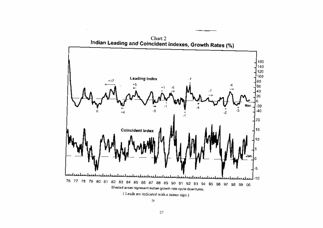
As Chart 1 and Table 1 show, the leading index had an average lead of 12 months at

business cycle peaks, zero months at troughs and six months overall. As Chart 2 and Table 2

show, the growth rate of the Indian Leading Index had an average lead of three months at

growth rate cycle peaks, zero months at troughs, and two months overall. These cyclical peak

and trough dates were determined on the basis of the classical algorithm (Bry and Boschan,

1971) developed at the National Bureau of Economic Research (NBER).

A closer look suggests that the leads were rather elusive until recent years (shaded

cells). Until the early 1990s, the leading index was roughly coincident with business cycles,

while the leading index growth rate was roughly coincident with growth rate cycles.

However, a clear pattern of leads has emerged in the last few years.

16

This experience is consistent with the logic of leading indicators, which is predicated

upon the existence of a free market economy. In the case of India, where the government had

long distorted the free market, such an assumption had questionable validity until economic

liberalization began in the early 1990s. Also, in earlier decades, a dominant agricultural

sector vulnerable to the vagaries of the monsoon made crop failures the key cause of

recessions. It is difficult for leading indicators to predict cyclical turns caused primarily by

such exogenous shocks.

Under such circumstances, it is understandable that the leading indicators did not lead

in a systematic manner, and also exhibited a number of extra cycles. However, a close look at

Chart 2 suggests that virtually all these extra cycles corresponded to smaller, roughly

contemporaneous fluctuations in the Indian Coincident Index introduced in Dua and Banerji

(1999), most of which did not exhibit the pronounced, pervasive and persistent declines that

mark true cyclical downturns.

What is clear is that the Indian economy grew at a relatively staid and steady pace in

the decades after independence, and recessions, which were caused mainly by bad monsoons,

were relatively shallow. Such behaviour was consistent with a command economy, where the

role of endogenous free market processes was limited and government action tended to

smooth out cycles.

6. LEADING INDICATORS IN A CHANGING ECONOMY

The Indian economy has changed profoundly in recent decades. The agricultural

sector, which accounted for over 50% of GDP until the early 1960s and over 40% of GDP

until the late 1970s, represented just 25% of GDP by the end of the 1990s. Meanwhile, the

spread of irrigation reduced the vulnerability of agriculture to the vagaries of the monsoon,

while a sustained nationwide build-up of buffer stocks of foodgrain broke much of the

linkage between crop failures and economic downturns. As a result, the Indian economy is

now far less dependent on good monsoons to sustain growth than it was earlier.

Separately, liberalization began in earnest in 1991 after a balance of payments crisis.

By the late 1990s, the economy had been partially liberalized and the leading indicators began

17

to show consistent leads, as in other free market economies (Table2). In fact, the average lead

of the Indian leading index growth rate in the two most recent growth rate cycles (shaded

cells) has improved to five months.

How much liberalization does it take, then, for leading indicators to start working? It

seems, based on our results, that after 1993 a sufficient degree of liberalization had occurred

for the leading index to show consistent leads. Consider the statistics shown in Table 1c.

The percentage of the time the leading index growth rate shows leads at growth rate

cycle turns has almost doubled to 100%. Meanwhile, the median lead has increased by 3.5

months and 11.5 months respectively at business cycle troughs and peaks, while it has

increased by 2.5 months and 5.0 months respectively at growth rate cycle troughs and peaks.

Does this mark a true shift in the behaviour of the leading index, or is it just a statistical

fluke?

It is important to note that it is not a simply a change in the relationship of the leading

index with the coincident index that is at issue here. The question is whether there is a

change in the behaviour of the leading index at business cycle and growth rate cycle turning

points. This is because the primary purpose of a leading index is to anticipate cyclical turns

in the economy, not necessarily to forecast economic conditions at other times.

Unfortunately, there is a very limited number of turning points that can be examined –

just six each at growth rate cycle peaks and troughs until 1993, and two each after 1993.

With such a small number of data points, it is not feasible to perform a parametric statistical

test that requires the estimation of parameters.

It is, however, possible to perform an appropriate nonparametric test (the

randomization test for two independent samples) that works for small samples of this sort

(Siegel, 1956). Despite the very small sample sizes, the changes between pre- and post-

liberalization performance are significant at the 0.067 level for growth rate cycle troughs, and

at the 0.200 level for growth rate cycle peaks. While more stringent significance levels are

normally used in statistical analysis, it is notable that even such levels of significance were

obtained given a sample size of just two in each case in the post-1993 period. While not

18

conclusive, this test therefore suggests, at least tentatively, that there was a shift in cyclical

behaviour in the early 1990s. In other words, the expected leads of the leading index do seem

to be emerging in the post-liberalization era.

7. CONCLUSIONS

The foundation for this research was the determination of business cycle and growth

rate cycles for the Indian economy, based on a traditional NBER-type approach. This earlier

research involved the creation of an index of coincident economic indicators, and the

determination of the reference chronologies based on a consensus of the turning points of this

index and its components.

An obvious approach might have been to start with a plausible set of leading

indicators, and check what worked well in predicting past cyclical turns. The problem,

however, was that the Indian economy had undergone major structural changes in recent

years, and past performance might have very little implication for future success.

Instead, we adopted a different approach inspired by the work of Klein and Moore

(1985) and Moore and Cullity (1994), as well as more recent work at ECRI on a wider variety

of economies, on robust sets of leading indicators. This work showed that, based on an

appreciation of the key drivers of the business cycle, it was possible to identify leading

indicators that were robust enough to work in a variety of market economies. Such sets of

roughly equivalent indicators are monitored monthly by ECRI for 16 countries including both

developed and developing economies, and have been shown to have good historical as well as

real time performance. This was the robust set of indicators used for India.

Since the Indian economy has been undergoing major structural changes in the

liberalization process, we believe that pre-liberalization performance may not be relevant to

the future success of the index. Instead, our approach has been to focus on the array of robust

leading indicators that work consistently in other market economies, and show that these are

now working in the Indian economy.

19

Clearly, what we are assuming by following this approach is that the new Indian

economy has more cyclical features in common with other market economies than with its

own earlier incarnation. Our consistent success in a variety of other market economies gives

us the confidence to adopt this approach. The results are consistent with this view – after all,

these same indicators work in country after country and also in the new Indian economy – but

do not work in pre-liberalization India.

Our procedure is at clear variance with more data-driven approaches. In any case,

there simply is not enough data in the post-liberalization period to try to fit the data in a way

that is likely to work in the future – and such an approach is risky, given the structural shifts.

In effect, what we have is an "out-of-sample" test for these same indicators that we have used

in many other countries, and it works in the period where it should be expected to.

Our results provide an indirect window into India’s progress towards a market

economy. In a sense, the emergence of leads since the mid-1990s is evidence that the free

market is starting to dominate the Indian economy. In this liberalized economy, it may be

expected that in spite of their indifferent record before the mid-1990s, the leading index and

its components will successfully anticipate future cycles in the Indian economy.

20

REFERENCES

Ashton, T.S. (1959), Economic Fluctuations in England, 1700-1800. Oxford:

Clarendon Press.

Banerji, A. (1999), “The Three P’s: Simple Rules for Monitoring Economic Cycles,”

Business Economics, XXXIV (4), 72-76.

Basu, K. (1992), “Markets, Laws and Governments,” in B. Jalan (ed.) The Indian Economy:

Problems and Prospects, New Delhi: Penguin Books.

Boschan, C. and A. Banerji (1990), “A Reassessment of Composite Indexes,” in P.A. Klein

(ed.) Analyzing Modern Business Cycles: Essays Honoring Geoffrey H. Moore.”

Armonk, NY: M.E.Sharpe.

_________ and W.W. Ebanks (1978), “The Phase-Average Trend: A New Way of Measuring

Growth,” Proceedings of the Business and Economic Statistics Section, American

Statistical Association, Washington D.C.

Bry, G. and C. Boschan (1971), Cyclical Analysis of Time Series: Selected Procedures and

Computer Programs, National Bureau of Economic Research, Technical Paper

No. 20, New York.

Burns, A.F. and W.C. Mitchell (1946), Measuring Business Cycles, National Bureau of

Economic Research, New York.

Chitre, V.S. (1982), “Growth Cycles in the Indian Economy,” Artha Vijnana, 24, 293-450.

_________ (1986), “Indicators of Business Recessions and Revivals in India,” Gokhale

Institute of Politics and Economics Working Paper.

Cullity, J.P. and A. Banerji (1996), “Composite Indexes: A Reassessment” presented at the

meeting on OECD Leading Indicators, Paris.

21

Dua, P. and A. Banerji (1999), “An Index of Coincident Economic Indicators for the

Indian Economy,” Journal of Quantitative Economics, 15, 177-201.

Klein, P.A. (1998), “Swedish Business Cycles – Assessing the Recent Record,” Working

Paper 21, Federation of Swedish Industries, Stockholm.

________ and G.H. Moore (1985), “Monitoring Growth Cycles in Market-Oriented

Countries, Developing and Using International Economic Indicators,” NBER Studies

in Business Cycles, No. 26, Cambridge, MA: Ballinger.

Layton, A.P. and G.H. Moore (1989), “Leading Indicators for the Service Sector,” Journal of

Business and Economic Statistics, 7, 379-386.

Mintz, I. (1969), “Dating Postwar Business Cycles: Methods and their Application to

Western Germany, 1950-67,” Occasional Paper No. 107, NBER, New York.

_______ (1972), “Dating American Growth Cycles,” in V. Zarnowitz (ed.), The Business

Cycle Today, NBER, New York.

_______ (1974), “Dating United States Growth Cycles,” Explorations in Economic Research,

1, 1-113.

Mitchell, W. (1927), Business Cycles: The Problem and its Setting,” National Bureau of

Economic Research Studies in Business Cycles, No. 1 and General Series No. 10.

Moore, G.H. (1950), Cyclical Indicators of Revivals and Recessions, National Bureau of

Economic Research, Occasional Paper No. 31.

Moore, G.H. (1982), “Business Cycles” in Encyclopaedia of Economics, D. Greenwald,

Editor in Chief, McGraw Hill Book Company, New York.

______ and J.P. Cullity (1994), “The Historical Record of Leading Indicators – An Answer

to ‘Measurement Without Theory’,” in K.H. Oppenlander and G. Poser (eds.) The

22

Explanatory Power of Business Cycle Surveys: Papers presented at the 21st CIRET

Conference Proceedings, Stellenbosch, 1993, Aldershot, UK: Avebury.

Niemira, M.P. and Klein, P.A. (1994), Forecasting Financial and Economic Cycles,

John Wiley & Sons, New York.

Siegel, S. (1956), Nonparametric Statistics for the Behavioral Sciences, New York:

McGraw-Hill.

Zarnowitz, V. and C. Boschan (1975), “Cyclical Indicators: An Evaluation and New Leading

Indexes,” in Handbook of Cyclical Indicators, Government Printing Office,

Washington, D.C.

23

Table 1Lead/Lag Record of Indian Leading Indexagainst Indian Business Cycle Chronology

Indian Business Cycle Indian Leading Index

Turning Points Turning Points Lead (-) / Lag (+) in Months

Troughs Peaks Troughs Peaks Troughs Peaks7/1977 extra

4/1979 2/1979 -23/1980 6/1980 3

4/1982 extra6/1983 extra

2/1985 extra4/1986 extra

3/1987 extra10/1987 extra

3/1991 12/1989 -159/1991 9/1991 0

5/1996 9/1994 -202/1997 12/1996 -2

Troughs PeaksOverall

0.0 -12.0Average-6.0

0.0 -15.0Median-2.0

50 100Percent Lead75

24

Table 2Lead/Lag Record of Indian Leading Index Growth

against Indian Growth Rate ChronologyIndian

Growth Rate CycleLeading IndexGrowth Rate

Turning Points

Troughs Peaks

Turning Points

Troughs Peaks

Lead (-) / Lag (+) in MonthsTroughs Peaks

2/1976 7/1975 -74/1977 extra

3/1978 extra9/1978 extra

1/1979 extra12/1979 12/1979 0

11/1980 1/1981 25/1981 extra

4/1982 extra2/1983 6/1983 4

8/1984 2/1984 -66/1984 extra

1/1985 extra4/1986 extra

3/1987 extra10/1987 10/1987 0

6/1988 6/1988 03/1989 2/1989 -1

3/1990 12/1989 -37/1990 extra

3/1991 extra9/1991 9/1991 0

4/1992 4/1992 07/1993 10/1993 3

4/1995 9/1994 -77/1995 extra

4/1996 extra2/1997 12/1996 -2

1/1998 7/1997 -610/1998 7/1998 -3

Troughs PeaksOverall

Average 0 -3-2

Median 0 -4.5-0.5

Percent Lead 56 7566

Average, 1994-99 -3 -7-5

Median, 1994-99 -2.5 -6.5-4.5

Percent Lead, 1994-99 100 100100

25

Table 3LLeeaadd(( -- )) //LLaagg((++)) ooff IInnddiiaann LLeeaaddiinngg IInnddeexx

aatt CCyycc ll ii ccaa ll TTuurrnniinngg PPooiinntt ss Until 1993 and Later

Median Lead atBusiness Cycle

Median Lead atGrowth Rate Cycle

Percent Lead atGrowth Rate Cycle

Period

Troughs Peaks Troughs Peaks Troughs Peaks1993 and earlier +1.5 -8.5 0.0 -1.5 42 67

After 1993 -2.0 -20.0 -2.5 -6.5 100 100

26

27

28