Embed Size (px)
Citation preview

Centre for Geo-Information
Thesis Report GIRS-2014-35
Cotton yield forecasting in Tashkent province by using Remote
sensing techniques
Djakhangir Atakhanov
24,
Septe
mber,
2014

ii

iii
Cotton yield forecasting in Tashkent province by using Remote
sensing techniques
Djakhangir Atakhanov
Registration number: 900327020060
Supervisors:
Dr. Ir. Jan Clevers
Dr. Alim Pulatov
A thesis submitted in partial fulfillment of the degree of Master of Science at Wageningen
University and Research Centre,
The Netherlands.
September, 2014
Wageningen, the Netherlands
Thesis code number: GRS-80436 Thesis Report: GIRS-2014-35 Wageningen University and Research Centre Laboratory of Geo-Information Science and Remote Sensing

iv
Acknowledgements
This study was benefited from constructive discussions and meetings with supervisor
Jan Clevers and Alim Pulatov. I would like to thank Alim Pulatov, for help with choosing the
Thesis topic, for discussions and expressing his knowledge about area and crop growth in study
area.
I would like to appreciate my fellow students who helped me during my thesis research
as well. Who helped with analysis and expressed me their experiences and gave me the hints to
find a solution and solve problems.
Two coordinators Ewa Wiestma and Alim Pulatov who helped to construct Double
degree program and gave me opportunity to be awarded by Erasmus Mundus CASIA 1 project
Action 2. I am thankful also for Wageningen University and Tashkent Institute of Irrigation and
Melioration for being involved for the scholarship. Moreover, I would like to appreciate all people
from both educational institutions for useful experience and knowledge.
MGI department and group, which were involved and supported me during my study and
research have to be appreciated as well. Their knowledge and experience in GIS and remote
sensing helped me and increased my level of knowledge.
I would like to thank my family and friends from home country for the help with obtaining
the data and useful information and for the great support and patience during three years of my
study.
I thank all state agencies, educational institutions and centers being involved in process
of delivering and providing me valuable, cognitive and important information. In addition, I would
like to appreciate the NASA USDA archive for providing images from diverse satellites.

v
Abstract
Crop yield forecasting is very important in every country around the world. Central Asian
countries are enriched with agricultural lands. Uzbekistan’s main sector is agriculture with a
large variety of different crops. Nowadays, 46% of all irrigated land is utilized for cotton. Cotton
is considered as most important crop in Uzbekistan. Production of cotton plays a dominant role
in the economy of Uzbekistan. Remote sensing assists to create information at a large spatial
scale. Therefore, it was used for prediction of cotton yield in Tashkent province, which has 15
administrative districts and 12 of them are located in the agricultural zone. The prediction was
made for Tashkent province (oblast) level and for the administrative district level. Classification
of cotton fields using MODIS (MOD13Q1) was applied by using a decision rule with thresholds
on the Normalized Difference Vegetation Index (NDVI) for day of the year 113, 161 and 225.
NDVI data was acquired as 16-day maximum value product in order to get information about
biomass condition. Different NDVI-based indicators were studied and analyzed in terms of
choosing the best option for that region. A regression model between NDVI indicators and yield
was applied using an overall temporal trend component and yearly deviations from this trend.
The temperature and precipitation were studied in order to find a relationship among yield, NDVI
and weather conditions. The correlations between these factors were low and it is assumed that
at least weekly observations of cotton are required for establishing a better correlation between
NDVI and weather conditions. Research has been successfully done and yield for 2013 was
predicted at the province level as well as at administrative districts level. Province level and
administrative district level showed difference in most valuable indicators, relationships between
weather conditions and yield and correlation between weather conditions and NDVI. As
indicators maximum value of NDVI and seasonal sum of NDVI (iNDVI=NDVI integral) were used
in this research. Results have shown that MODIS 250 m spatial resolution is not the most
suitable satellite sensor for Tashkent region and its administrative districts. In addition, there are
many varieties of fruits, vegetables and other crops that make it very difficult to classify and
make an error assessment of the classification and delineation of the cotton, as the cotton
growing calendar is similar to the one of other crops in the region. The results obtained at the
province level showed a decrease of yield in 2013 with 0.2 c\ha. The model was validated by
the leave-one-out cross-validation (LOOCV) procedure and the calculated RMSE for the model
at the Tashkent province level expressed a low value (RMSE=0.034), which means that error
was low. The best indicator was identified for the province level and for each administrative
district level separately, subsequently the forecasting was done for all research levels. Finally,
the correlation between the ground truth data (historical data) and NDVI forecasting was found
to be R2=0.55, which means that there was moderate correlation. Results obtained from this
research indicate that alternative satellites and indicators have to be assessed and analyzed.
The harvesting of the cotton and its time planning can be improved, as well as agricultural
management, in order to get better outcomes.

vi
Table of contents
Acknowledgements ...................................................................................................................................... iv Abstract ......................................................................................................................................................... v
Table of contents .......................................................................................................................................... vi
Abbreviations ............................................................................................................................................... vii
1. Introduction ........................................................................................................................................ 1
1.1. Background (Literature review) ..................................................................................................... 1
1.2. Yield prediction .............................................................................................................................. 2
1.3. MODIS data................................................................................................................................... 3
1.4. Problem Definition ......................................................................................................................... 4
1.5. Research Questions ...................................................................................................................... 4
1.6. Research objectives ...................................................................................................................... 4
2. Methods and Materials ...................................................................................................................... 5
2.1. Study Area ......................................................................................................................................... 5
2.2. Cotton ................................................................................................................................................. 6
2.3. Materials description .......................................................................................................................... 7
2.3.1. Methodology .............................................................................................................................. 7
2.3.2. MOD13Q1 Production ............................................................................................................... 9
2.3.3. NDVI Metrics description ........................................................................................................... 9
2.4. NDVI Analysis ............................................................................................................................. 10
2.5. Classification ............................................................................................................................... 11
2.6. Summary of methodology (Flow chart) ....................................................................................... 14
3. Results ............................................................................................................................................ 15
3.1. Tashkent Province (Oblast level) ................................................................................................ 15
3.1.1. Classification ........................................................................................................................... 15
3.1.2. Validation of the cotton raster layers ....................................................................................... 16
3.2. Yield analysis .............................................................................................................................. 18
3.3. NDVI Metrics ............................................................................................................................... 19
3.4. Results for administrative districts (District level) ........................................................................ 23
3.5. Validation of forecasting model ................................................................................................... 27
4. Discussion ....................................................................................................................................... 28
5. Conclusions and Recommendations .............................................................................................. 30
6. Reference list .................................................................................................................................. 32

vii
Abbreviations
AVHRR Advanced Very High Resolution Radiometer, LR-sensor on-board of the NOAA-
satellites
B Blue
CGMS Crop Growth Monitoring System, the combination of an agrometeorological crop
growth simulation model WOFOST, a database, and a yield prediction routine.
CropSyst Cropping System simulation model
DEM Digital Elevation Model
DOY Day of the Year
EOS Earth Observation System
EVI Enhanced Vegetation Index
fAPAR Fraction of Absorbed Photosynthetically Active Radiation
fPAR Fraction of Photosynthetically Active Radiation
GDP Gross Domestic Product
GIS Geographical Information System, software for storage of geographical data,
mostly in vector format
iNDVI NDVI integrated time series
LAI Leaf Area Index
LOOCV Leave-one-out cross-validation
MODIS Moderate Resolution Imaging Spectroradiometer
NASA National Aeronautics and Space Administration
NDVI Normalized Difference Vegetation Index. RS-indicator for amount of standing
vegetation
NIR Near infrared range of the spectrum, roughly from 780 nm to 1300nm
NOAA Series of near-polar satellites monitored by the US National Oceanographic and
Atmospheric Administration
NPP Net primary productivity
R Red

viii
Rell.eff. Relative efficiency
RMSE Root mean square error
PAR Photosynthetically Active Radiation
RS Remote Sensing: earth observation with imaging sensors on-board of
space/airborne platforms
SPOT Système Pour l’Observation de la Terre
USDA United States Department of Agriculture
UzHydromet Centre of Hydrometeorological Service at Cabinet of Ministers of the Rebublic of
Uzbekistan
WOFOST World Food Studies crop growth model, simulation model
VI Vegetation Index

1
1. Introduction
1.1. Background (Literature review)
Assessment and forecasting of crop yields are important for each country. Central Asian
countries are very rich of agricultural lands covered by various crops. Uzbekistan has the largest
sector of agriculture among five Central Asian countries. The economy of Uzbekistan mostly
depends on agriculture (Abdullaev et al., 2007). Agricultural accountings of Uzbekistan
economy cover about 30% of Gross Domestic Product (GDP), 40% of employment and 60% of
foreign exchange earnings (Abdullaev et al., 2007). There is 45 million hectares of land, where
60% of the land is used for agricultural purposes and 12% of this area are irrigated (FAO, 2003).
Cotton is the key crop in agricultural production of Uzbekistan. Other major cotton-producing
countries are USA, China, India, Pakistan, Uzbekistan, Turkey and Australia (Reddy et al.,
2000).
Nowadays, cotton is considered as the main crop on Uzbekistan agricultural lands and
its production plays a dominant role in Uzbekistan. Among all irrigated lands in this area, 46% is
covered by cotton (Zhou et al. 2007). Uzbekistan was considered as an important cotton-
growing region even in Russian Imperial times. The cotton lands were enhancing during the
Soviet Union, particularly after 1950. Main external influence to cotton yield is generally caused
by rainfall, temperature, incoming light, and nutrition. According to Muminov (1973), Central
Asia is an area with inadequate moisture and dry type of climate, therefore soil moisture is an
important factor for cotton yield evaluation in Central Asia. Water mainly is taken from two main
rivers, which are Amu Darya and Syr Darya. Amu Darya and Syr Darya are two main tributaries
of the Aral Sea (Abdullaev et al., 2007).
The estimation and forecasting of cotton crop yield is of importance for better targeting of
water resources, proper land-use planning, time management, proper use of labor forces,
enhancement of production and establishment of classification maps at a regional scale
(Ruecker et al., 2007). Remote sensing is one of the technologies which gives an unbiased
vision of large areas, provides spatial information and is widely used in assessment and
forecasting of crop yields at a regional scale (Doraiswamy et al., 2004). Satellite images allows
the accumulation of valuable information for the determination of relationships with ground truth
data by using spectral characteristics of the fields with expected harvest (Terekhov et al., 2007).
The normalized difference vegetation index (NDVI) is an indicator which uses visible and near-
infrared bands of the electromagnetic spectrum and can be useful for forecasting of crop yields.
A vegetation index such as the NDVI is adopted to analyze the remotely sensed measurements
and to assess whether the observed target contains live green vegetation or not.
Large size fields make it possible to use satellite information of medium resolution to
study the spectral characteristics of crops (Terekhov et al., 2007). Forecasting of the crop yield
can be based on empirical data using vegetation indexes, obtained from remote observation of
the fields that take place every year during the earing – flowering time (late July-early August).
According to Terekhov and Kauazov (2007), this period allows observation of the fields due to
the amount of green biomass and close relationship between the amount of plant and
productivity. Moreover, it can be a basis for forecasting model of crop yields. Aim of this
research is to forecast the cotton yield in Tashkent province by using remote sensing
techniques. The current methods of crop yield prediction in Uzbekistan are outdated. To renew

2
methods of prediction in Uzbekistan and in order to improve the time management and amount
of needed labor forces during the cotton harvest, accurate remote sensing prediction is needed.
Precise forecasting can be helpful not only for decreasing redundancy of time planning and
labor forces during cotton picking season, but also for good, accurate and statistically
straightforward prediction.
1.2. Yield prediction
Optical remote sensing techniques work sufficiently with agricultural systems, since
remote sensing provides information about actual status of plants at different stages of growth
through the reflectance and spectral signatures of a crop. This technique helps to identify crop
species of interest and also diseases, weed infestations, density, and other values of
agricultural variables (Soria-Ruiz et al., 2004). These variables can be used as an input for crop
growth models as yield indicators (Clevers et al., 1993). The status of a crop can be obtained by
using different indicators or vegetation indices like NDVI (Tucker, 1979).
There are different purposes for yield prediction in agricultural management. Among the
main goals are to categorize and forecast the amount of crop yield and to guarantee resources
for the population, obtained by agricultural and environmental services. Crop yield prediction for
large regions and for the period before the harvest time is rather an important and big problem
for many countries (Soria-Ruiz et al., 2004). Moreover, there are a lot of different models with
various issues associated with them (Soria-Ruiz et al., 2004), such as models which build and
rely on computer simulations and include weather-related variables. Other models are generally
statistical approaches which require several regression equations. In addition, there is no single
model, which can be suitable for all regions and environments. All crop growth prediction and
estimation models are limited to different conditions due to the reason that they were used and
simulated in specific research contexts and sometimes for areas as small as one field.
Moreover, they have to be used in combination with other inputs provided by various resources
such as geostatistical and geo-information systems (Soria-Ruiz et al., 2004).
Previous empirical studies were done to establish the statistical relationship between
crop yield and climate stresses. These studies had as purpose crop yield estimation and
prediction (Liang et al., 2012). The studies showed that the relationships are very complex and
depend on farming practices, climate and soil characteristics during the growing period.
According to Liang et al. (2012), weather conditions and soil characteristics have a strong
influence on cotton yield.
Different vegetation indexes were used, checked and developed in order to apply in one
of the existing models. Spectral vegetation indexes (VI) were used in order to measure the
green biomass at any given time. Satellite data such as NOAA-AVHRR (National Oceanic and
Atmospheric Administration – Advanced Very High Resolution Radiometer) and MODIS
(Moderate Resolution Imaging Spectroradiometer) have been used for different models run at
daily, monthly and yearly time step (Rucker et al. 2007a). Linear relationships were applied
between the fractions of photosynthetically active radiation (fPAR) and biomass of cotton. To
estimate the fPAR, NDVI was derived from AVHRR and the Monteith model was applied
(Bastiaansen, 2003). Moreover, different satellites and sensors have been extensively used to
monitor the condition of the crop and forecast crop yield and production in many different
countries. Studies were done to predict the yield by using remote sensing techniques.

3
Several studies by using a crop growth model instead of using the regression models
have been applied worldwide. One of the studies was done in order to predict yields using
meteorological information. The crop growth monitoring system was created for Europe and this
study led to the objective of another research, which was to monitor agricultural conditions over
the whole of the European Union and neighboring countries, and because of the importance of
wheat in Uzbekistan, the model was adapted there in order to make a quantitative within season
yield forecast at regional and national scale for specific crops by using the Crop Growth Monitor
System (CGMS) (Pulatov, 2008). Many studies have been performed using the AVHRR satellite
in order to monitor and forecast malting barley yield in Germany (Pulatov, 2008).
Many research works have been made in the last years to investigate the contribution of
remote sensing data for crop monitoring and yield prediction. In terms of forecasting the cotton
yield, MODIS (MOD13Q1) NDVI products have been used for Tashkent Province in this
research. The spatial resolution of MODIS is 250m per pixel. The research is aimed on
identifying the best indicator in order to predict cotton yield at Province (oblast) level and at
administrative district level. Forecasting of the yield can lead to better crop management, labor
forces and time management and to know whether this satellite is suitable and sufficient enough
for the scale of the field in the province.
1.3. MODIS data
According to the National Aeronautics and Space Administration (NASA), there is
MODIS (or Moderate Resolution Imaging Spectroradiometer) instrument, which is a key
instrument on aboard of TERRA and AQUA satellites (Lindsey & Herring, 2011). TERRA
satellite passes from north to south across the equator in the morning, while AQUA passes from
south to north and crosses the equator in the afternoon (Lindsey & Herring, 2011). TERRA and
AQUA MODIS acquire 36 spectral bands (Lindsey & Herring, 2011). MODIS is playing an
essential role in gathering global data and improve our understanding of global dynamics of land
surface and processes in the oceans and lower atmosphere. MODIS is a key instrument for
developing Earth System models able to monitor and predict the changes on the surface
(Lindsey & Herring, 2011).
In order to select a good model for cotton crop yield forecasting, a variety of studies on
this issue which were done in diverse countries were investigated and explored. Generally, use
of MODIS for crop yield estimation is often applied. The majority of studies have been
conducted in order to relate NDVI derived from MODIS with crop yield by monitoring the
vegetation conditions, drought, estimation and forecasting. The pros of MODIS are that it has
good spatial resolution (250m) and for example better radiometric calibration than AVHRR
(Mkhabela et al., 2011). In addition, studies on the relation of MODIS with crop yield have been
conducted in Uzbekistan but in another province, conditions and different environment
(Ruecker, 2007c). Another study, performed in China was done in order to test the suitability of
the methodology to estimate crop yield with MODIS NDVI on a regional level (Ren et al., 2008).
The study on the crop yield forecasting on Canadian prairies was taken as an example. The
objective of abovementioned study was to evaluate the possibility of using MODIS-NDVI to
forecast crop yield on the Canadian prairies and also to identify the best time for making a
reliable crop yield forecasting (Mkhabelaa, 2011). Additionally, another research on the near
real time prediction of corn yield in the U.S. was done using MODIS derived Wide Dynamic
Range Vegetation Index (WRDVI) (Sakamoto et al., 2014).

4
Based on the studies described, in terms of crop yield prediction by using MODIS
satellite, this research explained below is going to be done.
1.4. Problem Definition
The cotton harvest is time consuming and needs many labor forces. Due to outdated
methods of empirical forecasting, the amount of labor forces and needed time is unknown. The
redundancy of labor forces during the cotton harvest and weak time planning used for that,
takes a lot of financial and human resources. In order to improve the time management and
amount of labor forces, which are needed for the production of cotton, remote sensing based
yield forecasting will be done in this research as an example of Tashkent province in
Uzbekistan.
Nowadays, two most used approaches to forecast crop yield are the empirical
regression model and the biophysical crop model (Kogan et al., 2013). Currently, insufficient
input data are available in Uzbekistan for applying a dedicated cotton growth model. So, an
empirical regression model will be used in this research. It requires some selected predictors
such as a vegetation index derived from satellite images, meteorological data and historical data
of cotton yield in last 10 years (Kogan et al., 2013). Satellite data can provide continuous,
timely, human-independently information for large territories (Kussul et al., 2009).
The prediction of cotton yield may help farmers to improve the harvesting time, reduce
the risks, which they may meet with the production, and it also may help the government to
determine harvest plans strategically.
1.5. Research Questions
1. How can remote sensing prediction improve logistics of harvest in Tashkent province?
2. How accurate is the remote sensing prediction in comparison to ground truth data?
3. Which of the variables in NDVI metrics is valuable to identify the growing season?
1.6. Research objectives
1. Build statistical model for prediction of cotton yield
2. Validate the forecasting model
3. Determine the correlation between statistical data and remote sensing data
4. Identify the best variable for NDVI metrics
5. Study harvesting logistics in Tashkent province

5
2. Methods and Materials
2.1. Study Area
The study area of current research is Tashkent province (oblast) of Uzbekistan (Figure
1). Figure 2 illustrates the MODIS tile and the Tashkent province as an image.
There are 14 administrative districts: Bekobod, Bostanliq, Buka, Chinaz, Qibray,
Ohangaron, Oqqurgan, Parkent, Pskent, Quyichirchiq, Urtachirchiq, Yangiyul, Yuqorichirchiq
and Zangiota districts. Tashkent is the capital of the country and capital of the province, which
covers an area of 15300 sq. km. The major cities of the province are Angren, Olmaliq,
Ohangaron, Bekobod, Chirchiq, Tashkent, Yangiobod, and Yangiyul. The study was done for
the agricultural zone of the province. Agricultural zone contains not all the districts. As a result,
the analysis was done for Bekobod, Buka, Chinaz, Qibray, Oqqurgan, Pskent, Quyichirchiq,
Urtachirchiq, Yangiyul, Yuqorichirchiq and Zangiota districts (shown below in Figure 3). The
analysis and forecasting was done for all districts individually and at the province level as a
whole. The Tashkent province is bordered at the northeastern of Uzbekistan by ranges of
mountains named “Tian Shyan”. The main crops are cotton, grapes and grain cultivation, as well
as silkworm breeding, fruits and vegetables, cereals and citrus fruits are increasing. Substantial
parts of the province in the south and southwest are foothill flatlands. Tashkent features a
Mediterranean climate with strong continental climate influences. The weather in Tashkent is
characterized by cold and often snowy winters, but with long dry and hot summers. In total, the
winter consists of about 32 fully covered snowy days. Humidity level of air is around 56% on an
annual basis.
Figure 1 Digital Elevation Model representing Tashkent province location
Figure 2 Illustration of extent of Tashkent province on MODIS tile such as MOD13Q1
(250m)

6
Agricultural zone was taken as study area and the area covered by cotton was taken by
applying a pixel-based NDVI threshold classification on the agricultural zone. Threshold is
explained later in the classification section of the report. In Figure 3, the white color areas are
different administrative districts, which are located in the agricultural zone as explained before,
area with orange lines is an area not taken and not calculated for the prediction.
2.2. Cotton
Local varieties of cotton were planted in the study area. The sowing dates starting from
the beginning of April until the middle of May (Muminov, 1973). First harvesting was in the
middle of September.
According to Centre of Hydrometeorological Service at Cabinet of Ministers of the
Republic of Uzbekistan (UzHydromet), cotton is distinguished for 5 phases:
1. Planting
2. First square
3. Flowering
4. Accumulation of cotton bulb
5. Harvest
Figure 3 Agricultural zones and other area of Tashkent province.

7
Yields of cotton crop depend on the number of mature cotton bulb (balls) on the plant.
For the time of planting temperature plays a big role. The most suitable temperature to sow is
10 degrees °C (Muminov, 1973). Freezing also plays an essential role in the development of the
crop. Sometimes freezing can take place during the starting date of cotton growth,
subsequently requiring re-planting of big areas. According to Muminov (1973) first leaves
appear 10 days after sowing, if the temperature is larger than 10 degrees and next leaves start
to appear in 4-5 days range after first leaves. The rate of growth increases and becomes more
intense and leaves appear with intervals of 2-3 days. The agricultural management (fertilizer,
cultivation, crop rotation, soil organic matter, etc.) plays essential role in cotton growth and
productivity as well.
2.3. Materials description
In this study, following datasets were used:
- MOD13Q1 product of MODIS at 250m resolution for 2000-2013 years
- Yearly meteorological observations from 15 stations in Tashkent province for 2002-2013
- Historical data on cotton yields for Tashkent province for 2002-2013
- Historical data on cotton yields for all administrative districts in Tashkent province for
2002-2013
2.3.1. Methodology
A regression model was used as an approach to predict single dependent variable
(cotton yield) by a set of independent variables such as meteorological data and remote sensing
data.
The ground truth data (historical) were obtained from the State Statistics Committee of
Uzbekistan. This data, on cotton yield for the last 10 years, was used to predict the crop yield
and make a validation of the empirical prediction. Research was done at oblast (Province) level
and administrative district level. Oblast level is a sub-national administrative unit.
Satellite data such as MODIS were used, in order to test the suitability of spatial
resolution for Tashkent province and administrative districts of Tashkent province. Vegetation
index NDVI was derived from Terra MODIS satellite sensors product. MODIS product
MOD13Q1 was downloaded for whole period of planting-flowering-harvest. The months for
cotton calendar are approximated and determined as March-September. The MODIS product
MOD13Q1 will be described and introduced later in this report.
Meteorological data was obtained from the archive Uzhydromet. It includes information
from 15 meteorological stations of Tashkent province. All stations provide monthly
meteorological information such as precipitation, rainfall and average minimum temperature and
average maximum temperature.
All models were validated, calibrated and developed using official data on cotton crop
yield at province/oblast level for the period 2002-2013. I applied repeated procedure, which
means models were first calibrated and developed for the period 2002-2012 and forecasts
made for 2013 and 2014.
Linear regression model for cotton yield forecasting with use of satellite data derived
NDVI were applied. Statistical cotton yield data have been derived from the State Statistics

8
Committee of Uzbekistan for Tashkent province (2002-2013) and administrative district (2003-
2013).
The regression model shown below was used for yield representation:
Yi = Ti +dYi (1)
Where Yi is predicted yield, Ti is agricultural changes and in this study agricultural changes
were taken as a trend component of the yield during 11 years. Time series show yearly
changes, which can be compared with yearly NDVI and, moreover, it shows the deviation of the
yield. DYi is representing the difference of actual yield from the trend line (Kogan et al., 2013).
Deterministic component of trend Ti can be acquired from the equation below:
Ti = a+b (year) (2)
Where a is intercept of the trend and b is slope of the trend line of certain year.
Yearly variations have been estimated using the next regression model, which connects
the cotton yield dYi and NDVI.
dYi = Yi - Ti =f(NDVI)=b0+b1*NDVIij (3)
b0 and b1 was applied to include year effects (Street et al., 1988). NDVIij means NDVI indicator
such as maximum or integrated time series (Sum of NDVIij=iNDVI=NDVI integral) for some year
(i) and j represents the day of the year (DOY).
The deviations of NDVI during the growing season (14 times) for each year were
obtained in order to investigate the strength of the relationship with NDVI and to determine
whether the critical point has a strong correlation, when the crop productivity is highly sensitive
to weather conditions.
Leave-one-out cross-validation procedure was implemented for the prediction model. It
means that the forecasting model were developed for the years 2002-2012 at province level and
the years 2003-2012 at administrative district level (test data) in order to calibrate data for all
years except one. Therefore, for each province, each administrative district and each DOY for
which NDVI values are available, the n predicted values for cotton yield for testing data in this
case n=11 for province level and n=10 for administrative district level. Subsequently, after
calibration, model was used for the one left year (for instance 2013) to make a prediction for, in
this case, 2013. Validation was done by using the statistical data for 2013 obtained from State
Statistics Committee. In order to see the correlation between predicted value and statistical yield
this procedure was repeated for each year, meaning each run one year was left out of the
calibration and only used for validation. Afterwards, statistical data and predicted values were
compared.
Root mean square error (RMSE) was calculated, in order to see an error from the
forecasting model. To estimate the RMSE the official historical data and predicted data values
were used. RMSE was calculated by equation below (Kogan et al., 2013):
𝑅𝑀𝑆𝐸 = √∑((𝑃𝑖)−(𝑂𝑖))2
𝑛 , (4)
Where Pi and Oi are estimated yield data (Ti) and historical data of cotton crop, respectively. Ti
also can be determined as slow agricultural changes indicator.

9
2.3.2. MOD13Q1 Production
Global MODIS vegetation indices are designed to provide spatial and temporal data of
vegetation conditions. B, R, NIR reflectance were used to identify vegetation indices. MODIS
NDVI products provide us with time series for historical applications (USGS, 2014). MOD13Q1
has not only NDVI products but Enhanced Vegetation Index (EVI) products as well. EVI
maintains sensitivity at a dense canopy and minimizes variations of canopy background.
MOD13Q1 is computed from bi-directional surface reflectance and has been masked for clouds,
water, shadows etc. (USGS, 2014). In addition, the product data provides 250 meter pixel size
every 16 days. Due to its ease of application, simplicity and familiarity, VIs have wide range of
users (USGS, 2014), (Solano et al., 2010).
For more precise explanation of MOD13Q1 images downloaded by Julian days, Table 1
was created. It illustrates Julian days, which belongs to acquisition dates and the range of the
day acquired by MODIS satellite. Table 1 Illustration of downloaded MOD13Q1 images with NDVI for growing season available for 2002-2013
years
Day range Acquisition Date Julian Day
61-91 03.06 065
61-91 03.22 081
92-121 04.07 097
92-121 04.23 113
122-152 05.09 129
122-152 05.25 145
153-182 06.10 161
153-182 06.26 177
183-213 07.12 193
183-213 07.28 209
214-244 08.13 225
214-244 08.29 241
245-274 09.14 257
245-274 09.30 273
2.3.3. NDVI Metrics description
NDVI metrics are used to characterize the growing season under study. There are two
approaches to identify the growing period. Phenological metrics can be derived from satellite
data as a threshold-based approach and time-series of NDVI data using a curve derivative
method (USGS, 2011). The threshold-based approach use some values, which can be relative
or pre-defined values at which vegetation activity is assumed to begin. The timing and progress
of the plants may help researchers to make a conclusion about condition of the plants and their
environment (Reed et al., 1994). This study will derive the measures (metrics) from 10 years of
NDVI time series data within the period March-September. These NDVI time series data will be
derived from satellite data product MOD13Q1 with resolution of 250 m. Measurements with
NDVI metrics will provide information, which gives the ability to track the seasonal
characteristics of cotton more closely. NDVI indices will be obtained 14 times for 16-day periods

10
from March to September. Moreover, 14 data values are available for each of the 10 years,
which in total are 140 data values. The past efforts concluded assigning a threshold NDVI value
for the activity events of the plant (Reed et al., 1994). The NDVI values were investigated to
identify the photosynthetic activity and deceleration of photosynthesis. The metrics that may be
used as an indicator are shown in Figure 4:
Start of growing season (OnP)
End of growing season (EndP)
Duration of growing season (DurP)
Maximum NDVI during growing season (MaxV)
Time integrated NDVI during growing season (TINDVI)
Different indicators were described and studied in terms of precipitation and vegetation
dynamics. Two studies were done in two study areas in different climatic zones, but generally
with high amount of precipitation during the growing season of crops (Pulatov, 2008). Finally,
there was undertaken the investigation of the main driving indicators for prediction. Integrated
NDVI, which is equal to the sum of NDVI (iNDVI=sum of NDVI), is assumed as good indicator
for seasonal variation of different land types. In the current study, two indicators were taken in
order to see the relationship of NDVI to the yield and to predict the cotton yield in Tashkent
province and administrative district level. One of the best indicators is NDVI integral, which is
sum of the whole growing period (Kastens et al., 2005). This indicator can help to obtain the
acreage of the area by summation of the most greenness period, and it was found out that the
majority of yields is highly correlated with integrated NDVI summarized around the time of
maximum greenness (Tucker et al., 1980). The maximum NDVI and sum NDVI, which is the
integrated NDVI values over the year, derived from MODIS (MOD13Q1) provide with
information on yield prediction (Pulatov, 2008).
2.4. NDVI Analysis
NDVI values were taken for the Agro district of the Tashkent oblast for Julian days
shown in table 1. All 12 year images were obtained from archive of U.S. Department of Interior
Figure 4 Phenological metrics from temporal NDVI profile (Reed et al., 1994)
11
and Geological survey. NDVI analysis was done by choosing the proper and suitable indicators
(max, integrated time series shown in Figure 4). In addition, in order to obtain the cotton pixels
the thresholds were applied (explained in next section 2.5). The growing season was analyzed
between beginning of March and the end of September. Respectively, all NDVI indicators were
obtained for all years by repeating the whole growing season marked by Julian days. NDVI
indicators were analyzed by applying the threshold for certain Julian days in order to repeat and
suit the classification methodology of Platonov (2008) and Zhang (2011). Spectral signatures of
cotton for MODIS were studied and determined by analysis of Figure 6 (see next section).
Subsequently, certain dates were chosen and cotton was identified. During identification of
cotton pixels, the values of two different indicators were obtained, which helped to analyze,
understand and make calculation shown in results chapter.
2.5. Classification
Classification gives an opportunity to model an earth’s surface. Studies on this research
has a range of topics such as mapping of weed (Glenn, 2005); (Gokhale, 2006), modeling
wildfire (Ercanoglu, 2006), forecasting urban growth, and other applications. According to the
results of different scientists (Richards, 2005) classification accuracy depends on pixel’s location
similarities with training sites. Error assessment is a critical point in analysis and interpretation
process (Stehman, 1998).
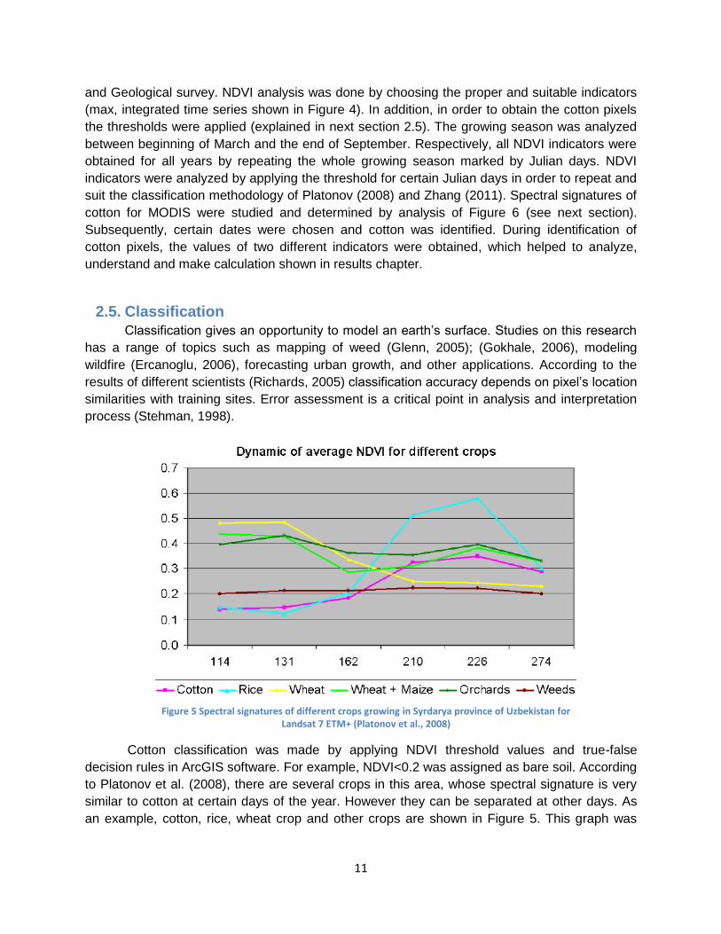
Cotton classification was made by applying NDVI threshold values and true-false
decision rules in ArcGIS software. For example, NDVI<0.2 was assigned as bare soil. According
to Platonov et al. (2008), there are several crops in this area, whose spectral signature is very
similar to cotton at certain days of the year. However they can be separated at other days. As
an example, cotton, rice, wheat crop and other crops are shown in Figure 5. This graph was
Figure 5 Spectral signatures of different crops growing in Syrdarya province of Uzbekistan for Landsat 7 ETM+ (Platonov et al., 2008)

12
shown in order to know the similarities of the spectral signatures for different crops in Syrdarya
area. Spectral signature used by Platonov was determined for Landsat ETM+ satellite.
In order to apply NDVI, threshold values and decision rules to MODIS suitable values
were explored and acquired. Figure 5 indicates that rice, cotton and wheat have very big
similarity during the growing season and at a certain DOY. For example, rice has similarities
with cotton spectral signatures on 110-114, 131, 160-162 Julian days and at the end of the
growing season has almost the same signature on 274 DOY, while wheat has close pattern with
cotton on 210, 226 and 274 DOY. So, to delineate cotton from other crops suitable values in
comparison with Landsat 7 ETM+ were applied (Figure 6). In order to differentiate cotton from
other crops the thresholds were examined from research done by Zhang (2011). That research
expresses the cognitive information about the values, which were applied as a threshold for
MODIS NDVI product, to obtain the cotton field pixels from the images. The NDVI thresholds
such as NDVI< 0.2 for 065-161 DOY have been applied. That value indicates bare soil. Second
threshold, which determines winter wheat-summer maize reflects the value such as NDVI> 0.35
and NDVI< 0.4 has been applied, moreover threshold for third critical point (225-273 DOY) of
the flowering and harvesting period of growing season is the period when maximum cotton
biomass reflectance have been caught. This period were indicated as NDVI > 0.63 and NDVI<
0.73. Last critical point helps us to get the spatially distributed cotton fields in that area (Zhang
et al., 2011). The most difficult part of acquisition was the end of growing season (225-273
DOY) when several crop signatures showed crossing or had similarities as shown in the
Platonov (2008) study. Then, some uncertainties had been discovered, such as absence of
required mean value in certain layer for certain DOY.
A pixel based threshold was applied to the images. Only three critical points had been
taken due to three critical periods as advised by Platonov (2008) (Figure 5) and Zhang (2011)
(Figure 6). Figure 5 was taken as an example of the differences of spectral signatures for the
different crops during the growing season in that area for Landsat ETM+. Meanwhile, Zhang
(2011) advised to use higher values for MODIS NDVI, which were applied for this research in
order to delineate cotton with the MODIS (MOD13Q1) NDVI product. The images cover the
growing season and have a frequency of one image close to the critical points of cotton spectral
Figure 6 Illustration of cotton, winter wheat-summer maize, and spring maize value MODIS NDVI temporal patters for China (Zhang et al., 2011)

13
signature such as April (113th day), June (161st day) and August (225th day). The limitations
have been met on this research for images of some days in certain year due to applied
thresholds. The issue of thresholds was not essential and were skipped at the moment of the
research. The problems were in insufficient values of threshold for a time when assumingly
cotton biomass, for instance, had maximum values at DOY 225, and in reality it has been less
than the minimum threshold which was applied for the certain days of certain year. More often it
has been met during the middle of the growing season. The classification gave NDVI values
with lower average pixel values spread out around the whole region. The threshold was done for
three images with NDVI by certain day of the year (NDVI DOY). The first moment was the
beginning of the growing season as 113th day of the year, when the temperature degrees are
equal or higher than the effective temperature (10 degrees Celsius). The minimum effective
temperature for cotton growth has to be equal to 10 degrees Celsius, which means cotton is not
growing in case of the less temperature. In order to record the period of wheat harvesting and
cotton sowing (bare soil), 113th day was applied. The second day has been taken as 161st day
of the year, which represents the middle of the growing season for the agricultural region.
Cotton biomass has not yet grown enough for the high VI values representation, but assumingly
it is possible to see the summer maize growth in order to divide these two crops from each
other. The last spot of the obtained NDVI data have been 225th day, which lies on August 13th
and can be counted as period with maximum NDVI value for cotton in Tashkent province level.
Data from day 65-273 for growing season was gathered for 10 years. 65-273 DOY
illustrates us the cotton growing calendar, which is expressed in Figure 6.
To check the accuracy of classification, geo-referenced points in Urtachirchik district
were taken as an example. All roads and cities were delineated from study area. The same
classification was done for each administrative district.
Validation for all regions was done by observations performed in Urtachirchik district.
GPS points taken by me in the summer of 2012 during my internship and additional GPS points
(coordinates), which were obtained by a first year master student of Tashkent institute of
Irrigation and Melioration, obtained during his internship in 2014 were used. According to
Platonov (2008), crops distributed over the area were recognized and validated with thresholds
applied to maps. Due to visible and recognizable fields of cotton in Google maps, it was
possible to check some area. The Urtachirchik administrative district was checked and validated
by control points obtained by GPS Leica Geosystems. Control points were done near cotton and
maize fields (Figure 9).
As an additional validation, the planted area from statistics was compared with the area
obtained from the classified cotton pixels using the NDVI thresholds. This comparison was done
by using data on planted area under cotton in ha. These data were obtained from Tashkent
statistical agency. Validation was done for all pixels for the whole agricultural area of Tashkent
province.

14
2.6. Summary of methodology (Flow chart)
Generally, the methodology of this research is followed by the flow chart indicated by the
conceptual model in Figure 7. There are two steps: first step is for oblast (province) level and
second step is for administrative district level. Each model has input and output. For instance,
software such as R and Microsoft Excel will be used to acquire NDVI metrics as a time series
with input from MOD13Q1 images of Tashkent province. Moreover, historical data obtained from
Uzbekistan will be analyzed in statistical graphs. Regression analysis will be done to compare
the output results collected from remote sensing and actual yield data. Results will be
represented by the yield forecasting after yield analysis. To see the amendments of NDVI
values, meteorological data were used and analyzed with the NDVI indicators.
Figure 7 Schematic overview of methodology at oblast level and district level

15
3. Results
3.1. Tashkent Province (Oblast level)
3.1.1. Classification
Thresholds used in the combination of DOY 113, 161 and 225 to identify cotton fields in
the various years are given in Table 2. Since the precise cotton distribution map is not available,
there are several different methods to check and validate the classification done in this research
(see section 3.1.2). As an example, raster layers acquired after applying the thresholds for the
signatures is shown for 2013 in Figure 8. Hereby, Figure 8 indicates three different days in three
different colors and blue considered as bare soil (113 DOY) while green color was applied for
the time of wheat harvesting. The time of wheat harvesting, which have been used for threshold
(161 DOY) is the same period as cotton sowing time. So, it means that green color illustrates
the cotton sowing period and wheat harvesting time. Finally, the red color was applied for the
period of 225 DOY, when the cotton biomass was reflecting the maximum NDVI values.
Table 2. Thresholds applied to identify cotton fields for specific DOYs
DOY NDVI
113 < 0.2
161 > 0.35 AND < 0.4
225 > 0.63 AND < 0.73
Figure 8 Cotton map distribution of cotton pixels in the study area for 2013 obtained after classification

16
3.1.2. Validation of the cotton raster layers
The major crops distributed over the agricultural zone in Tashkent province and NDVI of
crops consistent with the growing calendar of crops shown in Figure 5. The maximum NDVI for
wheat and other crops such as maize or orchard pixels is situated mainly on 161 DOY within the
given thresholds. In general, cotton pixels did not recognized on rainfed areas in Figure 8.
Control points obtained during my internship were used for validation of NDVI pixels in the study
area and showed that cotton fields at August 13th had highest NDVI value of 0.675 during the 12
years of study (2002-2013). As a comparison, according to Zhang (2011) 0.73 is the maximum
NDVI value, which was picked for cotton on their research. Red pixels illustrated in Figure 9
means that there are cotton fields on that area. The differences of the red color show
differences in amount of biomass of cotton due to weather and agricultural management
conditions (light tones represent less biomass). The points illustrated in Figure 9 expresses the
territory of study during the internship and points were obtained mainly near the cotton areas.
So, control points illustrate the fields covered nearby cotton fields and, for example, it is shown
that the left top point is located near the cotton field, which had not good green biomass at the
time image was taken. In general, all control points illustrate correct (meaning cotton) pixel
layers on the fields. In the middle of the shape of control points, there were potato, water melon
and other non-cotton, small fields, which correctly are not covered by any red pixels. On the
right hand of the shape, control points were taken in maize fields, which are not covered by
pixels as well. Six pixels illustrated on the bottom left are cotton as was discovered by the first
year student. On the top of the image it is unknown whether the cotton fields are correct.
The pattern was validated in order to compare the special critical days, meanwhile the
comparison showed good and almost similar pattern of cotton. As we can see on DOY 65,
which is 6th of March, the pattern is less than 0.2 and the minimum value on DOY 113, which is
Figure 9 Ground control points obtained by Leica GNSS and GPS systems in 2012 nearby cotton, maize,
orchards and other crops

17
0.000.200.400.600.80
ND
VI
Julian days
Comparison with pattern of Zhong (2011) to validate the classification
23rd April, is around 0.2 but increasing up to the maximum value (Figure 10), while maximum
NDVI value appeared at the same time as in the pattern mentioned by Zhang (2011), on 13th of
August (DOY 225). Those values show the similarities of the cotton pattern with Figure 6 and it
may be concluded that the classification was done appropriately.
The validation mentioned in the end of section 2.5 refers to the area covered by the cotton
pixels classified using the thresholds of table 2 for all the years as compared with the official
area statistics for cotton. Figure 11 shows that points are close to the 1:1 line for most years,
indicating that the threshold approach at least provides a good estimate of the total cotton area.
Deviations can be explained because some cotton fields can have a very low biomass, resulting
in a low NDVI value. The NDVI of cotton pixels was obtained after thresholds were applied.
Meanwhile, the obtained NDVI of pixels is the reflectance of greenness and non-greenness of
vegetation, which depends on solar radiation, photosynthetic activity (Ruecker, 2007), amount
of precipitation, water balance (Muminov et al., 1973), soil organic matter, soil bioactivity and
20
40
60
80
100
120
140
20 40 60 80 100 120 140
Pla
nte
d a
rea
(th
ou
san
d h
a)
NDVI pixel area (thousand ha)
Yearly planted area under cotton vs summarized NDVI pixel area
Figure 10 NDVI pattern for 2011 during four critical points indicates significance with the Zhang (2011) pattern of cotton.
Figure 11. 1:1 Relationship illustration comparing the planted area with NDVI area in thoiusand ha

18
other reasons, which can affect the presence of amount of chlorophyll of vegetation (Ruecker,
2007) or absence of biomass.
3.2. Yield analysis
The statistical data for the whole agricultural zone of Tashkent province expresses the
information, which is valuable for the objectives. Time series of the gross yield has a positive
trend line (Figure 12). Trend line was acquired by equation Y=0.4633x-905.69, where two
variables of trend is slope and intercept. Therefore, the slope is represented by value of 0.4633
and the interception is -905.69. In addition, Figure 12 interprets that in 2002, 2003 and 2008
yield was less than in other points of the time series. Moreover, maximum value was obtained
from 2006, continued by the decrease of the trend until 2008. Then it showed that in two last
years crop growth was decreasing. Afterwards, statistical yield data was compared with
temperature (Figure 13) to presume the influence of weather conditions to crop yield and see
the reason of low yield in some years. After the comparison of monthly average of temperature
with the yield, it interprets that there is no relationship (R2=0.01) with cotton yield (See below).
y = -0.0308x + 14.808R² = 0.0103
5.0
7.0
9.0
11.0
13.0
15.0
17.0
20.0 22.0 24.0 26.0 28.0 30.0
Tem
pe
ratu
re
Cotton Yield c\ha
Relationship among Temperature and cotton growth
Figure 12 Yield (c\ha) against time series for 12 years, Tashkent Province
Figure 13 Relationship between cotton gross yield (c\ha) and temperature average over 12 years

19
There is an assumption that, due to unavailable daily or weekly observations of cotton,
the relationship between variables is absent.
Precipitation in the study area mostly is in autumn-winter-beginning of the spring, while
cotton growth calendar starts in the end of March – beginning of April. Cotton is planted in
irrigated zones in Tashkent province and data such as monthly (growing season) or yearly
average of precipitation is not much playing a role in discovering relationship. The optimal
amount of precipitation for the cotton biomass is 5000-8000 m3\ha (Anonymous, 2014). But
generally, low amount of rainfall has to be fallen during the cotton growth, because at the same
time the amount of precipitation is valuable as well. If water content is not enough, cotton
biomass leave out the lowest layer of the boxes, in order to give the strength for the growth and
productivity to the rest (Anonymous, 2014).
Freezing has bad influence on cotton growth too (Muminov, 1973). Additionally, soil in
Central Asian region is inadequate (Muminov, 1973) and soil has to be moist during the seeding
period. This could be a reason of the low gross yield during 2007-2008 years. Assumptions are
that freezing was longer than usually, and farmers started cotton seeding later than usually.
No relationship trend line can be caused by applying the monthly average data obtained
from Uzhydromet rather than daily observations in the fields.
3.3. NDVI Metrics
The only two indicators studied in this research were the NDVImax and the NDVI
integral. The reason of using these two certain indicators are that different studies investigated
two indicators as the best indicators for such kind of studies and they are most essential for
forecasting.
Figure 14 NDVI max changes over 12 years for cotton

20
Figure 14 illustrates the time series of maximum NDVI values for cotton biomass over 12
years (2002-2013). Thus, changes illustrated in Figure 14 says that NDVI maximum indicator
varied not much and expresses very small range of changes during 12 year time series for
Tashkent province level. These small changes indicating negative decrease of an NDVI value
for cotton biomass, which leads to assumption that the temperature is increasing, which in its
turn can be observed in the statistical data and the biomass slightly became drier, and uniformly
lost chlorophyll content.
Figure 15 expresses NDVI integral (iNDVI) changes over 12 years. iNDVI shows wide
range in changes over 12 years and that graph has cognitive information for research. Figure 15
also illustrates the presence of agricultural changes as cotton growth increased and decreased
over 12 years in comparison with Figure 14. Figure 15 expresses that cotton NDVI integral is
decreasing over 10 years but for the last years the pattern shows development and increase,
which can be the influence of agricultural improvements. NDVI integral values is decreasing
from 2003 (4.890) then the maximum value was caught in 2008 (5.043) and shows more
temporal variability than the weather variability during 12 years.
The changes over 12 years of NDVI values shows that the cotton NDVI values are
decreasing, which means that biomass is not growing in some areas anymore or another
assumption is that farmers started to pay more attention to production of cotton boxes than to
growth of biomass. The causes of this kind of assumptions are that NDVI is the reflection of
greenness and non-greenness of vegetation, absence and presence of chlorophyll amount in
biomass, which is dependent on different variables (solar radiation, dry matter content, soil
organic matter, herbicides, fertilizers, water content), but not cotton bulbs (section 3.2.). The
increase of production in 2013 makes to think that predicted yield can be higher (Figure 15).
4.650
4.700
4.750
4.800
4.850
4.900
4.950
5.000
5.050
5.100
2002 2003 2004 2005 2006 2007 2008 2009 2010 2011 2012 2013
iND
VI
Year
NDVI integrated time series
Figure 15 Changes of NDVI integrated time series over 12 years

21
Figure 16 and 17 illustrate the relationship between the deviation of cotton yield from the
trend line and NDVI indicators. Both indicators at province (oblast) level showed weak
correlations (R2=0.0067 for maximum NDVI and R2=0.0838 for NDVI integral). There is an
assumption that there is an outlier in both graphs, whereas the indicator relationships with the
outlier included are shown. An outlier is interpreted as the maximum deviated point. iNDVI show
us an outlier with a big deviation on point, where deviation is equal to 4.31 and NDVI indicator is
equal to 4.9, while all other deviation values varying near trend line. The negative trend line can
be understood as the biomass reflectance was high and rich with chlorophyll content, while yield
(cotton boxes) production was low. It means that cotton plant was wet and did not produce the
cotton or production was later than usually, as biomass produces cotton boxes when the plant
becomes dry (Anonymous, 2014). In order to produce cotton, farmers increase dry matter
content with herbicides. So, assumptions are that herbicides were added to the biomass late
August or beginning of September. Generally, there is state standard for cotton growth
management, but each farmer can adjust these schemes according to his own circumstances
and conditions, i.e. skip one irrigation or change the date and time of agricultural input activity
due to weather condition or farmer circumstances (Anonymous, 2014).
For all levels the linear trend was chosen. The assumption consequently obtained after
studying Figure 16 and Figure 17 can state that NDVI indicators and MODIS satellites spatial
resolution of 250m is not the most suitable and good enough for the oblast level.
The best indicator for province level is stated as NDVI maximum, it became known after
RMSE value was calculated for all tested indicators. Obtained RMSE for NDVI maximum is
small and announcing a low value such as 0.14, which means that there is a weak error, and
accurate prediction can be done by using this indicator.
y = -70.003x + 46.719R² = 0.0067
-3.00
-2.00
-1.00
0.00
1.00
2.00
3.00
4.00
5.00
0.664 0.665 0.666 0.667 0.668 0.669 0.670 0.671 0.672
DYi
NDVI max
Illustration of yield deviation and NDVI max
Figure 16 Regression model for Tashkent province. Estimated parameters for Eq.(3) were b0=46.719 and b1=-70.003

22
The forecasting of the yield for 2013 is giving a positive result and it interprets that yield
will decrease in comparison with the previous year but cotton production increase. Figure 18
represents the predicted yield (red line) after using the LOOCV procedure. In order to see the
correlation between original yield and predicted yield the scatter plot Figure 19 is created. After
the LOOCV procedure was applied the prediction was fitted and done for 2013. Correlation
shows good relationship on Figure 19, which means that prediction is accurate.
0.0
5.0
10.0
15.0
20.0
25.0
30.0
20
02
20
03
20
04
20
05
20
06
20
07
20
08
20
09
20
10
20
11
20
12
20
13Pre
dic
ted
an
d o
bse
rved
yie
ld c
\ha
Year
Representation of predicted yield and observed data time series
Observed data
Predicted yield
y = -6.6608x + 32.624R² = 0.0838
-3.00
-2.00
-1.00
0.00
1.00
2.00
3.00
4.00
5.00
4.750 4.800 4.850 4.900 4.950 5.000 5.050 5.100
Dyi
iNDVI
Illustration of yield deviation and NDVI integrated
Figure 18 Illustration of predicted yield and original yield obtained from State Statistics Committee
Figure 17 Regression model for Tashkent province. Estimated parameters for Eq.(3) were b0= 32.624 and b1=-6.6608

23
3.4. Results for administrative districts (District level)
For each individual district various results and relationships between predicted yield and
observed (original) yield were found, but the strength of the relationships depended upon the
amount and quality of the imagery used. Figure 20 illustrates that cotton yield in Bekobod district
increases year by year. It also shows unexpected fluctuations in 2004-2005 and 2007-2008
years. Moreover, it can be stated that NDVI integrated performed well in the relationship with
yield deviation over 11 years for almost all districts. All districts show weak correlation, while the
strongest is for Bekobod district. It shows positive correlation and RMSE is 0.28 (Figure 24).
The linear trend indicates the performed correlation. The NDVI integrated indicator shows the
best results for Bekobod, Buka, Oqqurgan and Urtachirchik districts, while NDVI maximum
shows better results in other districts (table3). Several districts also had obstacles in this
y = 0.6409x - 1264.2R² = 0.3375
0.0
5.0
10.0
15.0
20.0
25.0
30.0
2002 2004 2006 2008 2010 2012 2014
Yiel
d c
\ha
Year
Hystorical data time series for Bekobod district
19.0
21.0
23.0
25.0
27.0
29.0
19.0 21.0 23.0 25.0 27.0 29.0
Ob
serv
ed d
ata
Predicted yield
Corelation between Statistical data and predicted yield
Figure 19 Relationship between original yield data obtained from State Statistical Committee
Figure 20 Historical data for Bekobod district. Estimated a0=0.6409 and a1=-1264.2 for that district as slope and intersect for Eq. (2)

24
research such as not complete set of historical data.
As an example, Bekobod district is taken and shown. The best indicator for that
district is iNDVI. The relationship shown in Figure 21 illustrates the deviation of the yield and
iNDVI, where it was explored very low with negative linear trend. Figure 21 expresses the
cognitive information such as illustration of the period when the production of the yield is high,
NDVI expresses low values, or when the yield is low but biomass reflectance is high. The
assumptions are that the agricultural management of cotton requires different inputs such as
herbicides, before harvesting to drive the biomass for drought. If biomass reflects well, the
assumption can appear such as there was rainfall in that area and cotton had increased water
content, which subsequently leads to less or late production while NDVI reflectance is high.
R² = 0.1807
-6.00
-4.00
-2.00
0.00
2.00
4.00
6.00
4.6500 4.7000 4.7500 4.8000 4.8500 4.9000 4.9500
DYi
NDVI integrated
Illustration of yield deviation and NDVI integrated
4.5000
4.6000
4.7000
4.8000
4.9000
5.0000
18.019.020.0
21.022.023.0
24.0
iND
VI
Tem
per
atu
re
Year
Illustration of temperature relationship with NDVI integrated in Bekobod district
Temperature mean iNDVI
Figure 21 Illustration of yield deviation and NDVI integrated
Figure 22 Temperature influence on NDVI integrated in Bekobod district

25
Comparison of the influence between weather conditions and NDVI (reflectance of
biomass) shows similarities from 2007. Meanwhile, temperature shows low relationship with
NDVI integrated. The reason could be that data used in this research, is an average of the
temperature for the growing season of the cotton (Figure 22), which means there are no critical
dates with high or low temperature inside. Positive correlation (Figure 23) with value of R2=0.34
indicates that there is correlation between temperature and cotton growth. According to
personal communication and interview (2014) with an anonymous interviewer, cotton growth
depends on an optimal temperature, and positive trend proves this statement. Statement says
that there is optimal temperature for good and normal tense of cotton growth. In case of
decrease and increase of the temperature, cotton plant decreases or stop growing.
R² = 0.3416
4.6500
4.7000
4.7500
4.8000
4.8500
4.9000
4.9500
20.0 20.5 21.0 21.5 22.0 22.5 23.0 23.5
iND
VI
Temperature mean
Illustration of temperature relationship with NDVI integrated in Bekobod district
15.0
20.0
25.0
30.0
15.0 20.0 25.0 30.0
Ob
serv
ed y
ield
Predicted yield
Correlation between predicted yield and observed historical yield
Figure 23 Correlation of the temperature and NDVI integrated in Bekobod district
Figure 24 Correlation between predicted yield (Yi) and observed yield

26
This district shows good relationship and RMSE is 0.28 between predicted yield and
observed yield (Figure 24). Figure 20 illustrates the historical data time series, which was
correlated with predicted date in Figure 24.
Table 3 illustrates the results of RMSE values estimation for all administrative districts of
Tashkent province. The most suitable for all regions, as was mentioned before, is NDVI
integrated. The correlation (R2) between predicted yield and observed yield is low for almost all
districts except the Tashkent province, which shows better results. Moreover, Bekobod and
Buka indicate the best results among all administrative districts.
Table 3 Results of Root Mean Square Error (RMSE) for all administrative districts in Tashkent province
MODIS (MOD13Q1) indicators
Name NDVI max NDVI
integrated R2
Tashkent province 0.14 0.16 0.45
Bekobod 0.31 0.28 0.47
Buka 0.02 0.005 0.51
Chinaz 0.08 0.12 No
correlation
Kybray NO NO No trend
Kuyichirchik 0.59 0.61 No
correlation
Oqqurgan 0.0078 0.0072 0.28
Pskent 0.054 0.12 0.28
Urtachirchik 0.007 0.002 0.25
Yangiyul NO NO No trend
Yukorichirchik 0.07 0.11 0.37
Zangiota NO NO No trend
The Best

27
Table 4 Illustrates overall results for all districts and all indicators. It expresses the predicted
yield in comparison with observed yield for 2013. The best results are shown for the NDVI
indicators and as correlation between predicted yield and observed yield are Buka, Oqqurgan,
Pskent, Urtachirchik and Yukorichirchik districts.
3.5. Validation of forecasting model
The validation at the province level and administrative district level was done for an
individual year. Root mean square error for Tashkent province and district level was calculated
for the calibration and validation with the results. The results indicate that predicted yield and
observed yield are relatively efficient. The correlation between all of the regions is shown in
Table 3 as R2. By the table and the results of RMSE done according to Eq.(4), it can be
concluded that cotton prediction can be done by using and validating this model. The accuracy
has been calculated as RMSE for the administrative districts as well.
Table 4 Illustration of all indicators for all distrits in 2013 predicted yield.

28
4. Discussion A cotton plant is dependent on many external variables like other crops in the study
area. In addition, cotton plant growth is very sensitive to various inputs and outputs. The results,
which were obtained by models in previous sections, proves it. The personal communication
helped to understand different aspects of this influence. There is a schematic plan, which is
called “technological map of cotton growth” (Ibragimov et al., 2007). According to interviews
(2014), cotton productivity depends on agricultural management.
Different farmers try to keep and follow the rules of the technological map, which
indicates proper and accurate cotton growth methods. In order to explore the influence of
weather conditions on cotton yield and the best NDVI indicator available from MOD13Q1
(MODIS NDVI product) for cotton yield prediction in the study area, regression models and
NDVI prediction models were applied. Due to different crops growing in Tashkent province, the
research needs to delineate the cotton fields from other crops. Classification methods were
applied and some obstacles during this step have been met. According to Platonov, for cotton
classification some thresholds can be applied. The reason of choosing that methodology was
that the research of Platonov was done in a neighboring province, but for the scale of a farm.
The plot made by Platonov gave information about different crops in the region growing at the
same time. Method of Platonov says that in order to classify cotton some decision rules (section
2.4.) can be applied. That method expresses that NDVI pixel value for DOY 113 should be <0.2,
which can be considered as bare soil or water. Then, NDVI pixel value was limited to <0.2 in
order to see rice spectral differences with cotton, as rice is growing at the same time and with
almost the same spectral signatures by DOY. Differences between cotton and rice can be seen
in section 2.4, where spectral signature of rice rises much higher during the period of the
maximum reflectance value of cotton (DOY 225). Previously mentioned DOY 225 has been
chosen in order to classify cotton from other crops as this day has to be the period when the
reflected MODIS NDVI value reflects maximum value, as NDVI at DOY 225 is <0.3 and NDVI at
DOY 225 is >0.5. After applying these thresholds and limits have been met, the question was
whether MODIS NDVI product needs the same NDVI values for the classification and the same
reflections for cotton as Landsat ETM+. Meanwhile, Zhang et al. (2011) stated that MODIS
pixels need higher thresholds for decision rule classification, as NDVI(@DOY113)>0.2,
0.35>NDVI(@DOY161)>0.4 and the latest critical point was NDVI(@DOY225)<0.63 and
NDVI(@DOY225)>0.73. Two methodologies were compared and the results in this research
showed similarities with Zhang’s methodology (Figure 6), where the thresholds for DOY were
taken from.
The reason of deviating outcomes was that cotton at that time had weak biomass, which
just had been grown up and not reflected a strong greenness value. In order to know it, the
thresholds were lower than at the end of cotton calendar and higher than at the beginning of the
growing calendar. So, results illustrated that due to different temporal and spatial resolutions of
both satellites thresholds to distinguish cotton biomass from rice, wheat and maize, has to be
different. MODIS NDVI values are higher than for the Landsat ETM+ satellite. In order to make
an assumption the MODIS spatial resolution and temporal range of images against the Landsat
temporal and spatial resolution were studied and taken into account.
The delineation of the cotton biomass from the rest drove us to more difficulties, as
wheat, maize, rice and cotton have the same growing calendar and the most similar spectral
signature has been studied between rice and cotton. The differences between them were

29
discovered only in one critical point at the end of the growing season for cotton plant and
harvesting time. This period is 225 DOY and acquisition date is equal to 13th of August. Rice
reflects much higher greenness than the cotton because rice is growing on the water, and water
increases the water content of the biomass. Meanwhile cotton is stopping to grow as farmers
apply different agricultural management, such as herbicide inputs in order to increase dry matter
content of the cotton (Anonymous, 2014). The reason of using the herbicides in the end of
cotton is that cotton flowers do not become boxes and seeds are not appearing as well as
cotton wool, when biomass is green and full of water content (Anonymous, 2014).
The reason of choosing the 225th DOY as a critical point is, that farmers chase the
cotton plants on July when 10-12th leaves have appeared in order to stop the growing strength
and drive the plant to give power to the flowers and bulbs. Subsequently, farmers irrigate the
fields in July as a last time (Ibragimov et al., 2007), in order to give water content and then start
to dry it (Anonymous, 2014). After chasing and increasing the water content, herbicides have to
be applied to increase dry matter content as was mentioned before. So, the period between
irrigation was done and herbicides are applied is DOY 225. In case of chasing time was delayed
the herbicides input will delay as well, which means that cotton will give good reflectance but
productivity will decrease (linear trend line illustrated in Figure 16 and Figure 17). Chasing time
and herbicides input time is dependent on money, labor forces, appropriate time management
and time of the last freezing in the beginning of the cotton calendar (Anonymous, 2014).
According to personal communication with the cotton classifier (2014), the results of NDVI
indicators for Tashkent province and for administrative district level leads to make an
assumption that current agricultural management is not leading to better outcomes or MODIS
NDVI indicators are not the most suitable for these regions. The reason of MODIS’
unsuitableness for this area is that the spatial resolution (250m) of the MOD13Q1 NDVI product
is too large to apply it on Tashkent province and district level. Because the fields in Tashkent
province are less than 60 ha (Djanibekov et al., 2010).
Different literature indicates that better classification can be made by using the cotton
distribution map or ground truth data in order to know the province and district. For this research
several points had been used in order to validate cotton fields and it illustrates (Figure 10) that
mostly cotton pixels lay on cotton fields and include other fields as well because of the
resolution of the satellite. In theory, the ideal approach for classification for the purpose of crop
yield forecasting the cotton distribution map is needed.
The optimal temperature for good cotton plant growth during the season is 25-30
degrees. Data used in order to find a correlation between weather conditions and cotton yield
were monthly and yearly averages for 12 years. Using monthly average data is not efficient for
such discovery. For finding better relationships, data has to be daily, because during the month,
there are critical temperatures and there might be critical days with precipitations, which are not
influence to an average number, and data represents small values. The weak negative
relationship between cotton yield and weather conditions helps to find explanations about
limitations and bottlenecks of cotton growth. Assumptions carry information not only in non-
sufficient and no quality data, but in addition it leads to an understanding of the impact of
weather conditions on the growth of cotton. In case the amount of precipitation increases the
adequate and optimal limit of good cotton growth or precipitation decreases below limit, the
cotton biomass stops growing and throw out the lower leaves, in order to give the strength to the

30
leaves on the top of the plant. It means the production will be low but plant will reflect well to the
sensors.
This research was done on a limited area, with restricted time range, with use of specific
methodology and model. Thus, this research might not indicate precise information for the
whole Republic.
5. Conclusions and Recommendations The prediction of the annual cotton yield can lead to knowledge of acreage under cotton
and of gross yield, which gives the opportunity to use proper logistics such as time planning the
amount of labor and others. Better schema of agricultural management will help to increase and
improve the production of the cotton, since cotton is very essential for Uzbekistan and is playing
one of the important roles of economy. The methods used in this research can help the
government of The Republic of Uzbekistan to create their own new-modern forecasting
methodology and improve time management on spending and planning the cotton harvest
(picking). The information and methodology helps to obtain cognitive information, which
subsequently might express the amount of labor forces needed in order to harvest and pick the
cotton without using excessive time and labor. Moreover, the results of this study could be
helpful in time management for use of another sensor in order to predict cotton yield by
accurately delineation of the cotton on that area. Therefore, this research expresses the
selection of other alternative indicators or satellites in order to forecast crop yield in Tashkent
province.
This forecasting used in this research for the cotton crop can effectively and accurately
lead to information about the amount of the yield before the harvesting time and gives to
farmers and others, the hints and the opportunity to make better, accurate and more efficient
cotton management and market decision with good time planning, and govern the harvesting.
The results show negative results for the prediction, which means that cotton product will
decrease in 2013, which is confirmed by historical data. This research leads to the assumption
that remote sensing prediction can transfer better and larger information than the ground truth
prediction because remote sensing gives information not only about crop yield, but it provides
more information such as vision of larger areas and subsequently helps to create the spatial
maps of the area. However, the most crucial things for precise prediction is to select and use
the good, suitable and sufficient indicators for the Tashkent region and moreover the better
sensors with lower resolution.
The best indicators for the province and its administrative districts are NDVI integrated
and NDVI maximum, which had been identified during the research. Other indicators should be
checked as different regions and different scales might require different variables. The districts,
which did not show good results, have to be studied better and more precisely in order to find
the most suitable sensor, model and indicator.
So, methods used in this research can conclude that farmers do not have enough
knowledge about production rather than to increase biomass, which in this case is cotton wools.
In addition, for better cotton prediction, there is need for a cotton distribution map or
ground truth data, which will help for more accurate cotton delineation from other crops.
However, classification was studied and learnt by literature review, which recommends cotton

31
NDVI values for MODIS sensors to apply decision rules. Classification was applied successfully
and it was concluded that other satellites have to be checked in that region as well because
cotton is growing on small scale fields. Therefore for better production, the transfer of
knowledge of the scientist has to be done and farmers have to study all schemes and
agricultural management to improve production. Farmers have to solve all obstacles and
problems to earn or take a loan from a bank to cover financial expenses such as for buying
fertilizers and herbicides, fuels and other costs. However, cotton growing procedure has to be
done according to state technological map (scheme for proper plant growth). This will lead to
better agricultural management, time planning and logistics.
More assumptions are that daily observations have to be done for temperature and
precipitation against cotton growth. Secondly, biweekly cotton observation has to be done in
order to see the influences of the daily changes of the temperature or precipitation instead of
comparing monthly measurements of temperature and precipitations against cotton gross yield,
which can show us the influence of weather conditions on daily growing and the time of
harvesting.
This research can help to understand cotton growth. Moreover, research can derive
valuable information such as to know the amount of data and the valuable data for prediction in
that area. Therefore, this study explains which indicators are the best ones for prediction in
Tashkent province level and at administrative level.
Before making any conclusions regarding cotton yield prediction in Tashkent province
and its administrative districts more research should be done, like collection of ground truth
data, time series analysis and cotton distribution mapping.

32
6. Reference list Abdullaev, I., Giordano, M., Rasulov, A. (2007). Cotton in Uzbekistan: Water and welfare.
Cotton sector in Central Asia (pp. 112-128). London: SOAS.
Anonymous. (2014, September 15). Personal communication with certified classifier of cotton.
(D. Atakhanov, Interviewer)
Asrar, G. Fuchs, M., Kanemasu, E.T., Hatfield, J.L. (1984). Estimating absorbed photosynthetic
radiation and leaf area index from spectral reflectance in wheat. Agronomy Journal 76,
300-306.
Bastiaanssen, W. G., & Ali, S. (2003). A new crop yield forecasting model based on satellite
measurements applied across the Indus Basin, Pakistan. Agricultural, Ecosystem and
Environment, Volume 94, Issue 3, 321-340.
Clevers, J.G.P.W., Bouwman, B., Buker, C., van Leuween, H.J.C. (1993). A conceptual
framework for estimating crop growth using optical remote sensing data. International
archive of phtogrammetry and remote sensing, 29, 18.
Djanibekov, N., Rudenko, I., Lamers, J.P.A., Bobodjonov, I. (2010). Pros and Cons of Cotton
Production in Uzbekistan: Case study #7-9. Ithaca, New York: Cornell University .
Doraiswamy, P.C., Hatfield, J.L., Jackson , T.J., Akhmedov, B., Prueger, J., Stern, A. (2004).
Crop condition and yield simulations using Landsat and MODIS. Remote Sensing of
Environment 92(4), 548-559.
Ercanoglu, M., Weber, K.T., Langille, J., Nevers, R. (2006). Modeling Wildland Fire
Susceptibility Using Fuzzy Systems. GIScience & Remote Sensing 43, №3, 268-282.
FAO. (2003). Fertilizer use of crop in Uzbekistan. Rome: Foor and Agricultural Organisation of
the United Nations.
Gallego, F.J., Carfagna, E., Peedell, S. (1999). The use of CORINE Land Cover to improve area
frame survey estimates. Research in Official Statistics 2 (2),, 99-122.
Glenn, N.F., Munt, T.J., Weber, K.T., Prather, T.S., Lass, L.W., Pettingill, J. (2005).
Hyperspectral data processing for repeat detection of small infestations of leafy spurge.
Remote Sensing of Environment 95, 399-412.
Gokhale, B., Weber,K.T. (2006). Modeling Cheatgrass using Quickbird Imagery. Final Report:
Detection, Prediction, Impact, and Management of Invasive Plants using GIS.
Goward, S.N., Markhan, B., Dye, D.G., Dulaney, W., Yang, J. (1991). Normalized difference
vegetation index measurements from the Advanced Very High Resolution Radiometer.
Remote sensing of Environment 35, 257-277.
Ibragimov, N., Evett, S.R., Esanbekov, Y., Kamilov, S.B., Mirzaev, L., Lamers, P.A.J. (2007).
Water use efficiency of irrigated cotton in Uzbekistan under drip and furrow irrigation.
Agricultural Water Management 90, 112-120.

33
Investopedia US, a. d. (2014). Investopedia US. Retrieved from (I) Investopedia web site:
http://www.investopedia.com/terms/p/polynomial_trending.asp
Kastens, J.H., Kastens, T.L., Kastens, D.L.A., Martinko, E.A., Lee, R.Y. (2005). Image masking
for crop yield forecasting using AVHRR NDVI time series imagery. Remote Sensing of
Environment 99 , 341-356.
Kogan, F., Kussul, N., Adamenko, T., Skakun, S., Kavchenko, O., Kryvobok, O., Shelestov, A.
Kolotii, A., Kussul, O., Lavrenyuk, A. (2013). Winter wheat yield forecasting in Ukraine
based on Earth observation, meteorological data and biophysical models. Journal of
Applied Earth Observation and Geoinformation, 23, 192-203.
Kussul, N., Shelestov, A., Skakun, S. (2009). Grid and sensor web technologies for
environmental monitoring. Earth science informatics 2(1), 37-51.
Liang, X.Zh., Xu, M. Gao, W., Reddy, K.R., Kunkel, K., Schmoldt, D.L., Samel, A.N. (2012).
Physical Modeling of U.S. Cotton Yields and Climate Stresses during 1979 to 2005.
Agronomy Journal, Volume 104, Issue 3, 675-683.
Lindsey, R., Herring, D. (2011). NASA Earth Observing System. Retrieved from NASA:
earthobservatory.nasa.gov
Mkhabela, M.S., Bullock, P., Raj, S., Wang, S., Yang, Y. (2011). Crop yield forecasting on the
Canadian Prairies using MODIS NDVI data. Agricultural and Forest Meteorology 151,
385-393.
Muminov, F.A., Karnaukhov, V.V. (1973). Methods of observing the cotton harvest. SARNIGMI.
Paruelo, J.M., Lauenroth, K.W. (1998). Interannula variability of NDVI and its relationship to
climate for North America Shrublands and grasslands. Biogeograhy 25, 721-733.
Platonov, A., Thenkabail, P.S., Biradar, Ch.M., Cai, X., Muralikrishna, G., Venkateswarlu, D.,
Cohen, Y., Alchanatis, V., Goldshlager, N., Ben-Dor, E., Vithanage, J., Manthrithilake,
H., Kendjabaev, Sh., Isaev, S. (2008). Water Productivity Mapping (WPM) Using
Landsat ETM+ Data for the Irrigated Croplands of the Syrdarya River Basin in Central
Asia. Sensors 8, 8156-8180.
Pulatov, B. (2008). Prediction of wheat yield in Uzbekistan by using the CGMS model and
SPOT-Vegetation data. Wageningen, The Netherlands: Wageningen University and
Research center.
Reddy, K.R., Hodjes, H.F., Kimball, B.A. (2000). Crop Ecosystem Responses to Climatic
Change: Cotton. In J. B. Nösberger, Climate change and global crop productivity (pp.
161-187). Wallingford: CAB International Publishing.
Reed, B.C., Brown, J.F., VanderZee, D., Loveland, Th.R., Merchant, J.W., Ochlend, D.O.
(1994). Measuring ohenological variablity from satellite imagery. Journal of Vegetation
Science 5(5), 703-714.

34
Ren, J., Chen, Zh., Zhou, Q., Tang, H. (2008). Regional yield estimation for winter wheat with
MODIS-NDVI data in Shandong, China. International Journal of Applied Earth
Observation and Geoinformation 10, 403-413.
Ressl, R. Dech, S.W., Ptichnikov, A., Novikova, N., Micklin, P., (1998). Desertification
monitoring and land use optimization in Aral Sea area with GIS. Geoinformationsysteme,
6:25-32.
Richards, J.A. (2005). Remote Sensing Digital Image Analysis. New York: Springer-Verlag.
Ruecker, G.R., Shi, Z., Muller, M., Conrad, C., Ibragimov, N. (2007a). Regional Scale
Estimation of Cotton Yield in Uzbekistan by Integrationg Remote Sensing and Field Data
into an Agrometeorological Model. Tashkent: Uzbekistan Cotton Research Institute.
Ruecker G.R., Wouter, A.D., Lamers,J., Ibragimov, N., Kienzler, K. (2007b). Regional
Estimation of Leaf Chlorophyll in Cotton in Uzbekistan by Upscaling a Vegetation Index
From Plant Scale to PROBA-1/CHRIS Hyperspectral Staellite Data.
Ruecker, G.R., Shi, Z., Muller, M., Conrad, C., Ibragimov, N., Lamers, J.P.A., Martius, C.,
Strunz, G., Dech, S.W. (2007c). Cotton Yield Estimation in Uzbekistan Integrating
MODIS, Landsat ETM+ and Field Data. 123-129. Khorezm province, Uzbekistan.
Sakamoto, T., Gittelson, A.A., Arkebauerc, T.J. (2014). Near real-time prediction of U.S. corn
yields based on time-series MODIS data. Remote Sensing of Environment 147,, 219-
231.
Solano, R., Didan, K. Jacobson, A., Huete, A. (2010). MODIS Vegetation Index User’s Guide.
Arizona: The University of Arizona.
Soria-Ruiz, J. Fernandez-Ordonez, Y., Granados-Ramirez, R. (2004). Methodology for
prediction of corn yield using remote sensing satellite data in Central Mexico.
Investigaciones Geograficas, Boletin del Instituto de Geografia, UNAM, 55, 61-78.
Stehman, S.V.. Czaplewski, R.L. (1998). Design and Analysis for Thematic Map Accuracy
Assessment: Fundamental Principles. Remote sensing and environment 64, 331-344.
Street, J.O., Carroll, R.J., Ruppert, D. (1988). A note on computing robust regression estimates
via iteratively reweighted least squares. American Statistician 42, 152-154.
Terekhov, A.G., Kauazov, A.M. (2007). Sub-satellite MODIS-oriented analysis informative
vegetation indices for the description of the state of spring wheat in Northern
Kazakhstan. Modern problems of remote sensing of the Earth from space 2(4), 352-357.
Tucker, C.J., Holben, B.N., Elgin, J.H.Jr, McMurtrey, J.E. (1980). Relationship of spectral data
to grain yield variation. Photogrammetric Engineering and Remote Sensing 45, 657-666.
Tucker, C.J. (1979). Red and photographic infrared linear combinations for monitoring
vegetation. Remote Sensing of Environment, 8(2), 127-150.

35
USGS. (2011, January 06). USGS Science for a changing the world. Retrieved from USGS
Science for a changing the world: http://phenology.cr.usgs.gov/methods_deriving.php
USGS, (2014, April 14). Retrieved June 17, 2014, from LAND PROCESSES DISTRIBUTED
ACTIVE ARCHIVE CENTER: https://lpdaac.usgs.gov
Zhang, Sh., Lei, Y., Wang, L., Li, H., zhao, H. (2011). Crop Classification Using MODIS NDVI
Data Denoised by Wavelet: A Case Study in Hebei Plain, China. China Geografical
science, 21(3), 322-333.
Zhou, Sh., Ruecker, G.R., Shi, Z., Muller, M., Conrad, C., Ibragimov, N., Lamers, J.P.A.,
Martius, C., Strunz, G., Dech, S.W., Vlek, P.L.G. (2007). Modeling of Cotton Yields in the
Amu Darya River Floodplains of Uzbekistan Integrating Multitemporal Remote Sensing
and Minimum Field Data. Agronomy Journal 99(5), 1317-1326.