CEO Horizon, Optimal Pay Duration, and the

Escalation of Short-termism∗

Ivan Marinovic† Felipe Varas ‡

April 27, 2018

Abstract

This paper studies optimal CEO contracts when managers manipulate their per-

formance measure, sometimes at the expense of firm value. Optimal contracts defer

compensation. The manager’s incentives vest over time at an increasing rate, and

compensation becomes increasingly sensitive to short-term performance. This process

generates an endogenous CEO horizon problem whereby managers intensify perfor-

mance manipulation in their final years in office. Contracts are designed to foster

effort while minimizing the adverse effects of manipulation. We characterize the opti-

mal mix of short- and long-term compensation along the manager’s tenure, the optimal

vesting period of incentive pay, and the resulting dynamics of managerial short-termism

over the CEO’s tenure. Our paper provides a rationale for issuing stock awards with

performance-based vesting provisions, a practice increasingly adopted by U.S. firms.

∗We thank Jeremy Bertomeu, Tim Baldenius, Peter Cziraki, Alex Edmans (discussant), Simon Gervais,Ilan Guttman, Zhiguo He, Francois Larmande (discussant), Gustavo Manso (discussant), Ross Morrow,Adriano Rampini, Florin Sabac, Alex Storer, Vish Vishwanathan, and Jaime Zender (discussant) for helpfulcomments and seminar participants at Alberta (Canada), Duke University (Fuqua), Bocconi, NYU, SFSFinance Cavalcade, Tilburg, FIRS Conference, Texas Finance Festival, WFA, U. of Vienna, U. of Mannheim,and the 10th Accounting Research Workshop for their helpful feedback.

†Stanford University, GSB. email: imvial@stanford.edu‡Duke University, Fuqua School of Business. email: felipe.varas@duke.edu

1

Disclosure Statement

I have nothing to disclose.

Ivan Marinovic

I have nothing to disclose.

Felipe Varas

2

1 Introduction

Short-termism is prevalent among managers. Graham, Harvey, and Rajgopal (2005) find

that 78% of U.S. CEOs are willing to sacrifice long-term value to beat market expectations.

For example, Dechow and Sloan (1991) argue that, by the end of tenure, CEOs tend to cut

R&D investments which, though profitable, have negative implications for the firm’s reported

earnings. Managerial short-termism has been an important concern for many years, but it

has assumed a particularly prominent role in recent years following the Enron scandal and

the financial crisis in 2008.

To understand this phenomenon, the theoretical literature has adopted two approaches.

One approach studies CEO behavior, taking managerial incentives as given, and thus it is

silent about optimal incentives (see e.g., Stein (1989)). However, the complexity of CEO con-

tracts in the real world (which include accounting-based bonuses, stock options, restricted

stock, deferred compensation, clawbacks, etc.) suggest that shareholders are aware of CEO’s

potential manipulations and design compensation to mitigate the consequences of such ma-

nipulations. An alternative approach studies optimal compensation contracts that are de-

signed to fully remove CEO manipulations. In this class of models, manipulation is not

observed on the equilibrium path (Edmans, Gabaix, Sadzik, and Sannikov (2012)). This

approach is particularly helpful in settings in which CEO manipulations are too costly to

the firm or easy to rule out, but it cannot explain why manipulation seems so frequent in

practice or why real world contracts may tolerate them or even induce manipulation (see

Bergstresser and Philippon (2006)).

We study optimal compensation contracts when CEOs exert hidden effort but can also

manipulate the firm’s performance to increase their compensation, sometimes at the expense

of firm value. Building on Holmstrom and Milgrom (1987), we consider a setting with a risk-

averse CEO, who can save privately and consume continuously, and who exerts two costly

actions: effort and manipulation. Both actions increase the CEO’s performance in the short

run, but manipulation also has negative consequences for firm value. As in Stein (1989),

we assume these consequences are not perfectly/immediately captured by the performance

measure but rather take time to be verified, potentially creating an externality when the

CEO tenure is shorter than the firm’s life span.

Our paper makes two contributions to the literature. First, on the normative side, we

3

study the contract that maximizes firm value in the presence of manipulation. We character-

ize the optimal mix of long- and short-term incentives, the duration of CEO pay throughout

CEO tenure, and the ideal design of clawbacks and post-retirement compensation. Second,

on the positive side, we are able to make predictions about the evolution of CEO manip-

ulations along CEO tenure, and we establish the existence of an endogenous CEO horizon

problem.

We study the timing of manipulation: how it evolves over the CEO tenure and whether

optimal contracts may generate a horizon effect in which the CEO distorts performance

at the end of his tenure. Previous literature has shown that in dynamic settings one can

implement positive effort and zero manipulation at the same time (unlike in static settings)

by appropriately balancing the mix of short- and long-run incentives. However, in our

setting, inducing zero manipulation is not optimal; rather, tolerating some manipulation

is desirable because, in return, this allows the firm to elicit higher levels of effort than a

manipulation-free contract. Furthermore, to fully discourage manipulations, the firm would

have to provide the CEO with a large post-retirement compensation package that ties his

wealth to the firm’s post-retirement performance. Such post-retirement compensation is

costly to the firm, as it imposes risk on the CEO during a period of time when effort does

not need to be incentivized, and the CEO must be compensated for bearing this extra risk

(see, e.g., Dehaan et al. (2013)).

In the absence of manipulation, short-term incentives, measured as the contract’s pay-

performance sensitivity (PPS), are constant over time, as in Holmstrom and Milgrom (1987).

Unfortunately, the simplicity of this contract vanishes under the possibility of manipulation.

A constant PPS contract is no longer optimal because it induces excessive manipulation,

particularly in the final years in office. Indeed, offering the CEO a stationary contract would

lead him to aggressively shift performance across periods, boosting current performance at

the expense of firm value. To mitigate this behavior, an optimal contract implements lower

levels of short-term compensation and higher levels of long-term compensation, measured,

roughly, as the present value of the contract’s future slopes.

Also, in the absence of manipulation, the CEO incentives vest deterministically, but,

under the possibility of manipulation, vesting is contingent upon firm performance. This is

empirically relevant. Bettis, Bizjak, Coles, and Kalpathy (2010) assert that, even though

restricted stock awards with time-vesting provisions historically account for the majority of

4

performance-based pay in U.S. companies, shareholder advocacy groups and proxy research

services have expressed concern that these provisions do not provide sufficiently strong in-

centives and have suggested that compensation contracts should include performance-based

vesting conditions. In fact, since the mid-1990s, U.S. firms have increasingly issued option

and stock awards with sophisticated performance-based vesting conditions. Our paper pro-

vides a rationale for this phenomenon. Under the possibility of manipulation, the optimal

contract defers compensation and includes performance-based vesting provisions. In the ab-

sence of manipulation, the vesting date of incentives is known at the start of the CEO’s

tenure, and it is independent of the firm’s performance. When the CEO can manipulate

performance, the optimal contract includes performance-based vesting. Thus, the duration

of incentives is random: vesting accelerates with positive shocks and is delayed with neg-

ative shocks. Random vesting is helpful in the presence of manipulation because it allows

the principal to change the level of long-term incentives without having to simultaneously

distort the short-term incentives to avoid creating an imbalance, which would trigger extra

manipulation. Hence, performance-based vesting provides the principal with an additional

degree of freedom to reduce the CEO’s long term incentives without having to distort effort

to contain manipulation.

The optimal contract also includes a post-retirement package that ties the manager’s

wealth value to the performance of the firm, observed for some time after his retirement.

This contracting tool is helpful but has limited power when the CEO is risk averse: even

when the firm has the ability to tie forever – and to any degree – the manager’s wealth to

the firm’s post-retirement performance, the contract generally induces some manipulation.

Although it would be possible to defer compensation long enough to deter manipulation

altogether, firms might not do so, given the cost. A key insight in this paper is that firms

find it more beneficial to defer compensation while the CEO is still on the job rather than

after he retires. This result implies that long-term incentives are larger at the beginning of

the CEO’s tenure and decay toward the end.

Under the possibility of manipulation, optimal CEO contracts are non-linear, unlike in

Holmstrom and Milgrom (1987). Following Edmans et al. (2012), we first characterize the

optimal contract within the subclass of contracts that implement deterministic sequences of

effort and manipulation. Under such deterministic contracts, long-term incentives and effort

are intertwined. Long-term incentives can be reduced only via increasing the current slope

5

of short-term compensation, which necessarily distorts the level of effort. This is why, in

general, the optimal contract implements incentives that are path dependent. The benefit

of providing stochastic incentives which are history dependent and lead to stochastic effort

and manipulation, resides precisely in allowing the principal to control the evolution of long-

term incentives independently of the CEO’s effort. We find that at the beginning of the

CEO’s tenure, the performance sensitivity of long-term incentives is close to zero. However,

towards the end of the tenure, such sensitivity becomes negative; positive shocks accelerate

vesting thereby reducing long-term incentives. Generally, we find that long-term incentives

are mean reverting and follow a target level. If, due to their stochastic nature, the long-term

incentives increase relative to its target, the sensitivity of long-term incentives with respect

to shocks becomes negative, in order to drive the long-term incentives back down.

Related Literature Beginning with Narayanan (1985), Dye (1988), and Stein (1989), a

large number of studies in accounting, economics, and finance have examined the causes

and consequences of performance manipulation in corporate settings. Most of the literature

studying managerial short-termism has either taken incentives as exogenously given (Stein

(1989); Fischer and Verrecchia (2000); Guttman et al. (2006), Kartik, Ottaviani, and Squin-

tani (2007)) or has restricted attention to static or two-period settings with linear contracts,

which are unsuited for studying the dynamics of short-termism and its relation to optimal

long-term incentives (Baker, 1992; Goldman and Slezak, 2006; Dutta and Fan, 2014; Peng

and Roell, 2014). A related strand of the literature examines optimal compensation con-

tracts in the presence of moral hazard and adverse selection (Beyer et al. (2014); Maggi and

Rodriguez-Clare (1995); Crocker and Slemrod (2007)).

A more recent literature stream studies dynamic contracts under the possibility of ma-

nipulation (Edmans, Gabaix, Sadzik, and Sannikov, 2012; Varas, forthcoming; Zhu, 2018).

These studies restricts their attention to contracts that prevent manipulation altogether.

Because we are interested in making predictions about the evolution of short-termism, we

consider more general contracts that implement optimal levels of manipulation. Sabac (2008)

studies CEO horizon effects in a multi-period model with renegotiation where effort has

long-term consequences. He finds that effort can decrease while incentive rates increase as

managers approach retirement. DeMarzo et al. (2013) study a dynamic agency model where

the CEO can take on “tail risk,” thereby gambling with the firm’s money. The optimal con-

6

tract must strike a balance between providing effort incentives and controlling the manager’s

risk-taking behavior. The authors show that when the manager’s continuation value reaches

low levels, due to poor performance, the manager engages in excessive risk taking.

On the technical side, we borrow heavily from Holmstrom and Milgrom (1987), Williams

(2011), He, Wei, and Yu (2014), and Sannikov (2014). The problem of managerial short-

termism is closely related to the long-run moral hazard problem in Sannikov (2014), and we

model the inter-temporal effect of the CEO’s action in a similar way as Sannikov (2014).

In Sannikov (2014), the future CEO’s productivity is determined by today’s effort, so long-

term incentives are required to incentivize effort today. He et al. (2014) studies the design

of long-term contracts when the manager’s ability is unknown and learned over time and

shows that a combination of private saving and CARA utility provides great tractability to

analyze dynamic contracting problems with persistent private information.

2 Model

We study a dynamic agency problem where the agent (hereafter, CEO) can manipulate the

firm’s performance to boost his own compensation. The CEO exerts two costly actions,

effort at and manipulation mt. The principal observes neither action but a noisy measure of

firm performance.

Let {Bt}t≥0 be a standard Brownian motion in a probability space with measure P, and

let {Ft}t≥0 be the filtration generated by B. For any Ft -adapted effort, at, and manipulation,

mt, processes, the firm’s cash flow process is given by

dXt = (at +mt − θMt)dt+ σdBt

Mt =

∫ t

0

e−κ(t−s)msds,

whenMt is the stock of manipulation accumulated through time t. The stock of manipulation

Mt reduces the firm cash flows; at each point, the marginal effect of manipulation on the

firm cash flows is −θ. At the same time, the stock Mt depreciates at rate κ; this means that

the consequences of manipulation are more persistent when κ is smaller. Also, as θ vanishes,

manipulation ceases to have future cash-flow consequences as it is qualitatively equivalent

to effort.

7

This representation of short-termism goes back to Stein (1989) and captures the idea

that manipulation may increase current cash flows but eventually destroys firm value. The

accounting literature refers to this behavior as real earnings management. Some examples of

this behavior arise when managers cut advertising expenditures or R&D to boost reported

earnings, offer excessive discounts to meet earnings expectations; or risk the firm’s reputa-

tion by lowering product quality/safety. More generally, we can think of manipulation as

any potentially unproductive actions aimed at boosting the firm’s short-run profits. Notice

that unlike effort, manipulation is inherently dynamic: it increases today’s performance but

decreases the firm’s cash flows in future periods. In a nutshell, manipulation is a bad in-

vestment, or a mechanism the manager might use to borrow performance from the future to

boost current performance.1

Following Holmstrom and Milgrom (1987), we assume that the CEO has exponential

preferences given by

u(c, a,m) = −e−γ(

c−h(a)−g(m))

/γ,

where h(a) ≡ a2/2 and g(m) ≡ gm2/2. By assuming that manipulation is costly to the

manager, we thus follow the literature on costly state falsification (Dye, 1988; Fischer and

Verrecchia, 2000; Lacker and Weinberg, 1989; Crocker and Morgan, 1998; Kartik, 2009).

The cost of manipulation g(m) captures the various personal costs the CEO bears from

manipulating the firm’s performance. These costs include the effort required to find ways of

distorting cash-flows, litigation risk, fines imposed by the SEC, or the natural distaste from

behaving unethically.2 We allow the cost parameter g to be zero, which captures the case

when manipulation is costless.

The CEO is infinitely-lived but works for the firm for a finite time period, t ∈ [0, T ].

We refer to T as the manager’s retirement date, and to T − t as his horizon at time t. We

assume the contract can stipulate compensation beyond retirement, until time T + τ for

τ ≥ 0. In other words, the manager’s compensation can be made contingent on outcomes

1Prior literature (see Dutta and Fan (2014)) has modeled the reversal of manipulation as taking place inthe second period of a two-period setting. Although not fundamental, one of the benefits of our specificationis its flexibility to accommodate different reversal speeds. In our model, the effect of manipulation vanishesgradually based on κ. As we shall see, this parameter is a key determinant of the manager manipulationpatterns.

2This last interpretation is consistent with introspection and existent experimental evidence (Gneezy,2005).

8

observed after his retirement. This possibility captures the principal’s ability to implement

a clawback: a longer τ represents an environment where clawbacks can be enforced for a

longer period of time.

In practice, T is random. For tractability reasons, we assume that the retirement date

T is known. One can think of T as an approximation to some predictable separation date.

For example, Cziraki and Xu (2014) find that CEO terminations are mostly concentrated

around the end date of their contracts. The CEO’s expected utility given a consumption

flow {ct}t≥0 is

U(c, a,m) = E(a,m)

[∫ T

0

e−rtu(ct, at, mt)dt+

∫ T+τ

T

e−rtuR(ct)dt+ e−r(T+τ)uR(cT+τ )

r

]

,

where uR(c) ≡ u(c, 0, 0) is the flow utility accrued to the CEO after retirement. Notice again

that the CEO tenure is finite but the principal effectively controls the CEO’s compensation

over his entire life, even after T + τ. As will become clear, this assumption make it possible

to study the effect of changes in the contracting environment while holding the CEO’s life

expectancy constant. By doing so, we remove dynamic effects on the structure of the CEO’s

compensation driven merely by the shortening of the period length available to pay the CEO

as he grows old. Edmans et al. (2012) show that with a finite life, pay-performance sensitivity

rises over time as the number of periods to pay the agent his promised compensation is

reduced. The same would be true in our setting if we assumed the CEO’s life ends at T + τ .

Following He et al. (2014), we assume that the CEO can borrow and save privately –

that is, a hidden action – at the common interest rate r. This possibility allows the CEO

to smooth consumption intertemporally and hence restricts the ability of the principal to

implement compensation schemes that lead to steep expected consumption patterns. Being

able to privately save and borrow, the CEO can smooth consumption over time.

The principal designs the contract to maximize firm value. A contract is a consumption

process {ct}t≥0 and an effort-manipulation pair {(at, mt)}t∈[0,T ] adapted to the filtration

generated by the performance measure Xt. Formally, the principal chooses the contract to

maximize the present value of the firm’s discounted cash flow net of the CEO’s compensation,

as given by

V (c, a,m) = E(a,m)

[∫ ∞

0

e−rt(

dXt − ct1{t≤T+τ}dt)

− e−r(T+τ)cT+τr

]

.

9

The firm value is thus equal to the discounted net stream of cash flows, which includes a

terminal bonus granting the manager a consumption flow cT+τ from time T+τ onward (these

are the CEO pension benefits).

We assume that the negative long-run effect of manipulation dominates the instant bene-

fit, so manipulation destroys value. In other words, manipulation is a negative NPV project.

Using integration by parts we find that

E

[∫ ∞

0

e−rtdXt

]

= E

[∫ T

0

e−rt(at − λmt)dt

]

,

where λ ≡ θr+κ

− 1 captures the value-destroying effect of manipulation. When θ is large

relative to r+κ, manipulation is detrimental to firm value – yet potentially attractive to the

manager. In other words, manipulation destroys value when either the stock of manipulation

Mt is highly persistent (i.e., r + κ is small) or the marginal effect of Mt on the firm current

cash flows is large (i.e., θ is large). Throughout the paper, we make the following parametric

assumption.

Assumption 1. θ ≥ r + κ.

If θ = r + κ, that is if λ = 0, then manipulation has no cash flow effect; it only shifts

income across periods, being akin to accrual earnings management. In contrast, if θ > r+κ,

(λ > 0), then manipulation not only shifts cash flows across periods but also destroys firm

value, being akin to real earnings management.

The principal’s expected payoff given (ct, at, mt) is

V (c, a,m) = E

[∫ T

0

e−rt(at − λmt)dt−

∫ T+τ

0

e−rtctdt− e−r(T+τ)cT+τr

]

.

3 The CEO’s Problem

In order to solve for the optimal contract, we first characterize the CEO’s behavior given

an arbitrary contract. We state the CEO’s problem given an arbitrary contract, state the

necessary incentive compatibility constraints, and provide an informal discussion of these

conditions. After describing the necessary conditions for incentive compatibility in Propo-

sition 1, we provide a formal analysis of the CEO’s optimization problem and derive these

10

conditions using the stochastic maximum principle.

The CEO can save and borrow privately. We denote by St the balance in the CEO’s

savings account, so given an arbitrary contract prescribing actions (ct, at, mt) the CEO solves

the following problem:

supc,a,m U(c, a, m)

subject to

dXt = (at + mt − θMt)dt+ σdBt

dSt = (rSt − ct + ct)dt, S0 = 0.

(1)

We rely on the first-order approach to characterize the necessary incentive compatibility

constraints: that is, we characterize incentive compatibility by looking at the first order

conditions of the CEO’s problem. We verify the sufficiency of the first-order conditions later

on in Section 7.

As is common in dynamic contracting problems, we use the CEO’s continuation utility,

Wt as a state variable in the recursive formulation of the contract. The continuation utility

can be written as

Wt = Et

[∫ T+τ

t

e−r(s−t)u(cs, as, ms)ds+ e−r(T+τ−t)uR(cT+τ )

r

]

. (2)

The contract stipulates the sensitivity of Wt to cash flow shocks, dWt/dXt, as captured by

the slope of incentives, which we denote by −Wtβt. We refer to βt as the contract pay-

performance sensitivity.

Often in models of dynamic contracting, the continuation value is a sufficient statistic;

however, in our setting, manipulation has a persistent effect on the firm’s performance. Thus,

the CEO’s incentive to manipulate is tied to the manager’s expectation of the contract’s

future pay-performance sensitivities, βt. Because of the persistent effect of manipulation, we

need to include an additional state variable that measures the impact of manipulation on

future outcomes. This inter-temporal effect is captured by the state variable pt given by

pt = Et

[∫ T+τ

t

e−(r+κ)(s−t)dWs

dXsds

]

. (3)

11

When choosing manipulation, the CEO faces a trade-off between boosting current compen-

sation and lowering future compensation. The latter effect is discounted by the interest rate

r and the “depreciation rate” of the manipulation stock, κ.

The presence of long term-incentives is crucial to attenuate manipulation. When the

CEO inflates dXt by an extra dollar, he expects compensation to go down in the future,

as the manipulation reverses, more so the larger the CEO’s long-term incentives pt become.

The speed κ and intensity θ of the manipulation reversal determines how much effort the

CEO will exert before resorting to manipulation.

The contract also specifies how long-term incentives pt react to shocks, namely, the

performance sensitivity of long-term incentives, which we denote by σpt.

We can now state the necessary incentive compatibility constraint. In Section 7 we return

to the issue of sufficiency.

Proposition 1. A necessary condition for the contract (ct, at, mt) to be incentive compatible

is that for any t ∈ [0, T ]:

rγh′(at) = βt (4a)

g′(mt) = φptWt

+βtrγ

if mt > 0 (4b)

g′(mt) ≥ φptWt

+βtrγ

if mt = 0, (4c)

where φ ≡ θrγ

and (Wt, pt, βt, σpt)t≥0 solves the backward stochastic differential equation

dWt = −σβtWtdBt, WT+τ =uR(cT+τ )

r(5a)

dpt =[

(r + κ)pt + βtWt

]

dt + σσptWtdBt, pT+τ = 0. (5b)

Finally, the private savings condition requires that for any t ∈ [0, T+τ ] consumption satisfies

rWt = u(ct, at, mt). (6)

The previous result states necessary incentive compatibility constraints using the first-

order approach. It remains to prove that the first-order approach is valid so the above

conditions are sufficient. We address this issue in Section 7. Equation (4a) states that the

12

CEO’s marginal cost of effort must equal the sensitivity of his continuation utility to perfor-

mance βt, which captures the CEO’s marginal benefit of effort. This condition is analogous

to the incentive compatibility constraint in a static setting with linear contracts, which states

that the marginal cost of effort is equal to the slope of incentives. Equations (4b)–(4c) are

analogous incentive constraints for manipulation: The marginal cost of manipulation equals

the marginal benefit of manipulation. The latter has two components: i) a positive compo-

nent capturing the extra compensation the manager gets by manipulating the performance

measure today βt, and ii) a negative component capturing the decrease in future compen-

sation arising from the reversal of future cash flows triggered by manipulations, which is

proportional to pt in equation (3). This represents the negative effect in present value that

today’s manipulation has on future payoffs. Equations (5a)–(5b) provide the evolution of

the state variables (Wt, pt), which is derived in the appendix. Equation (6) is a consumption

Euler equation arise as a consequence of the private savings assumption and the absence of

wealth effects under CARA preferences. The Euler equation for consumption implies that

the marginal utility of consumption is a martingale while CARA utility implies that the

marginal utility is proportional to the current utility. Hence, which means that the cur-

rent utility ut equals rWt, so the continuation value Wt is a martingale (its drift is given by

rWt−ut = 0). As He et al. (2014) point out, for general utility functions, allowing for private

savings introduces an additional state variable, but this is not the case in a CARA setting,

where the marginal value of savings is proportional to the level of current utility. Introduc-

ing private savings greatly simplifies our problem and the characterization of the optimal

contract. When the agent cannot smooth consumption, the principal chooses the agent’s

consumption to control the ratio between the agent’s current utility and his continuation

value to provide incentives.

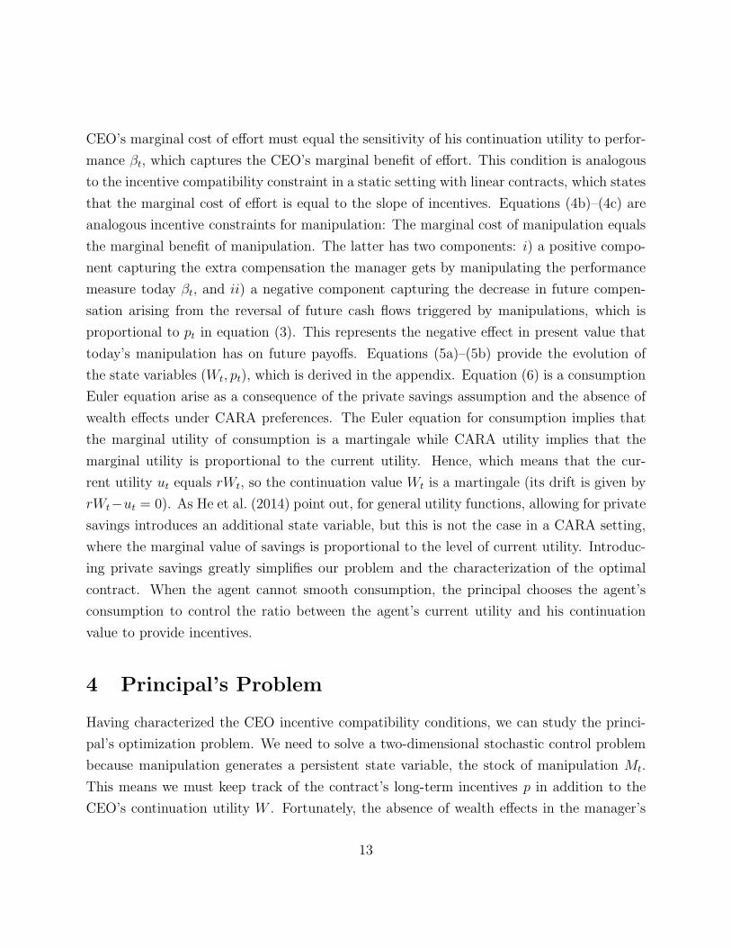
4 Principal’s Problem

Having characterized the CEO incentive compatibility conditions, we can study the princi-

pal’s optimization problem. We need to solve a two-dimensional stochastic control problem

because manipulation generates a persistent state variable, the stock of manipulation Mt.

This means we must keep track of the contract’s long-term incentives p in addition to the

CEO’s continuation utility W . Fortunately, the absence of wealth effects in the manager’s

13

CARA preference, along with the possibility of private savings, allows us to work with a

single state variable, as we shall demonstrate.

The principal’s original optimization problem can be written as follows:

V (W0, p0) = supc,a,m,β,σp V (c, a,m)

subject to

dWt = −σβtWtdBt, WT+τ =uR(cT+τ )

r

dpt =[

(r + κ)pt + βtWt

]

dt+ σσptWtdBt, pT+τ = 0

rWt = u(ct, at, mt)

IC constraints (4a)-(4c).

In principle, we need to keep track of two state variables, W and p. However, using the

properties of CARA preferences under private savings, we can rewrite the principal’s op-

timization problem as a function of a single state variable: zt ≡ −pt/Wt. This variable

represents the contract’s long-term incentives p scaled by the agent’s continuation utility W .

We can think of z as measuring the importance of deferred compensation (e.g., the number

of equity grants that will vest in the future, scaled by the total continuation value of the

CEO). From now on, we refer to zt as long-term incentives.

Before reformulating the principal’s problem, notice that the private savings condition

immediately pins down the manager’s consumption process as, given by:

ct = h(at) + g(mt)−log(−rγWt)

γ. (7)

Given private savings, consumption depends on the CEO’s continuation value, effort, and

manipulation, so we do not need to consider it as a separate control variable. This further

simplifies the formulation of the problem.

Lemma 1. The principal value function can be written as

V (W, p) = constant+log(−rγW )

rγ+ F

(

−p

W

)

,

where, defining z ≡ −p/W , F (z) solves the maximization problem

14

F (z) = supa,m,β,σz

E

[∫ T

0

e−rt (at − λmt − h(at)− g(mt)) dt−

∫ T+τ

0

e−rtσ2β2

t

2rγdt

]

(8)

subject to the incentive compatibility constraints (4a)–(4b), and the law of motion for zt

dzt = [(r + κ)zt + βt(σσzt − 1)]dt+ σztdBt, zT+τ = 0, (9)

where σzt ≡ σ(βtzt − σpt).

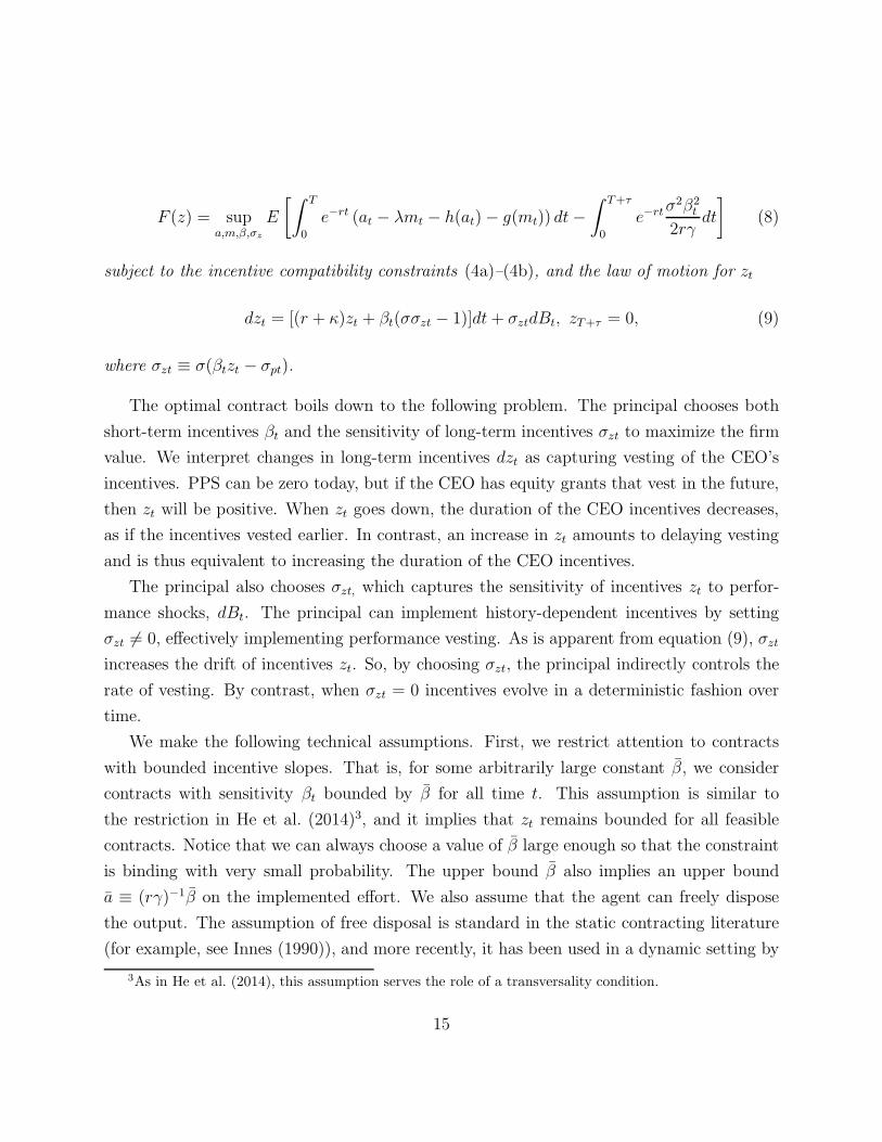
The optimal contract boils down to the following problem. The principal chooses both

short-term incentives βt and the sensitivity of long-term incentives σzt to maximize the firm

value. We interpret changes in long-term incentives dzt as capturing vesting of the CEO’s

incentives. PPS can be zero today, but if the CEO has equity grants that vest in the future,

then zt will be positive. When zt goes down, the duration of the CEO incentives decreases,

as if the incentives vested earlier. In contrast, an increase in zt amounts to delaying vesting

and is thus equivalent to increasing the duration of the CEO incentives.

The principal also chooses σzt, which captures the sensitivity of incentives zt to perfor-

mance shocks, dBt. The principal can implement history-dependent incentives by setting

σzt 6= 0, effectively implementing performance vesting. As is apparent from equation (9), σzt

increases the drift of incentives zt. So, by choosing σzt, the principal indirectly controls the

rate of vesting. By contrast, when σzt = 0 incentives evolve in a deterministic fashion over

time.

We make the following technical assumptions. First, we restrict attention to contracts

with bounded incentive slopes. That is, for some arbitrarily large constant β, we consider

contracts with sensitivity βt bounded by β for all time t. This assumption is similar to

the restriction in He et al. (2014)3, and it implies that zt remains bounded for all feasible

contracts. Notice that we can always choose a value of β large enough so that the constraint

is binding with very small probability. The upper bound β also implies an upper bound

a ≡ (rγ)−1β on the implemented effort. We also assume that the agent can freely dispose

the output. The assumption of free disposal is standard in the static contracting literature

(for example, see Innes (1990)), and more recently, it has been used in a dynamic setting by

3As in He et al. (2014), this assumption serves the role of a transversality condition.

15

Zhu (2018). The free disposal imposes a non-negativity constraint on βt. This means that

we restrict attention to contracts that have a sensitivity βt ∈ [0, β] before retirement.

5 Infinite Tenure and Irrelevance of Manipulation

What is the role of the retirement date T on the structure of CEO pay? As a benchmark,

here we study the case with T = ∞. We start with a variation of the moral-hazard-without-

manipulation problem studied by Holmstrom and Milgrom (1987) but allow for both interme-

diate consumption and private savings. This problem serves as a benchmark for evaluating

the effect of short-termism on the optimal contract.

In the absence of manipulation (namely when the manager cannot manipulate the per-

formance measure), deferring compensation beyond T plays no role; hence, zT = 0 and the

principal’s problem boils down to

maxat

E

[∫ T

0

e−rt(

at − h(at)−σ2rγh′(at)

2

2

)

dt

]

.

The principal can optimize the agent’s effort point-wise, which yields

aHM ≡1

1 + rγσ2.

aHM is the optimal effort arising in the absence of manipulation concerns, as Holmstrom

and Milgrom (1987) have shown (this is also the level of effort arising in the case without

learning studied by He, Wei, and Yu (2014)). We have thus confirmed that under CARA

preferences and Brownian shocks the optimal contract is linear and implements constant

effort over time.

In practice, the benefits of non-linear contracts are controversial. The executive com-

pensation literature often argues that firms should get rid of non-linearities in compensation

schemes to prevent performance manipulation. For example, Jensen (2001, 2003) argues that

non-linearities induce managers to manipulate compensation over time, distracting them

from the optimal long-term policies. Consistent with this view, we show that even when

manipulation is possible, the above linear contract remains optimal as long as the CEO

works forever. More precisely, we show that when T = ∞, the optimal contract is linear

16

and induces no manipulation. In fact, a perpetual linear contract aligns the incentives of

the principal and the CEO, eliminating his incentive to manipulate performance over time.

Later on we show that a no manipulation contract is no longer optimal when T < ∞, even

though it might still be feasible.

The no manipulation constraint can be written as follows:

βt − θEt

[∫ ∞

t

e−(r+κ)(s−t)βsWs

Wtds

]

≤ 0.

If pay-performance-sensitivity, βt, is constant, then the no manipulation constraint can be

reduced to

β

(

1− θ

∫ ∞

t

e−(r+κ)(s−t)ds

)

≤ 0

becauseWt is a martingale. In turn, this is always satisfied under the condition that manipu-

lation has negative NPV, as stated in Assumption 1 (i.e., θ ≥ r+κ). Hence, we have verified

that, under infinite tenure, the optimal contract in the relaxed problem that ignores the pos-

sibility of manipulation continues to be feasible when the manager is allowed to manipulate.

When the manager’s tenure is infinite, the possibility of manipulation is thus irrelevant and

the optimal contract implements no manipulation, being thus identical to that in Holmstrom

and Milgrom (1987). We summarize the previous discussion in the following proposition.

Proposition 2. When θ ≥ r + κ and T = ∞ the optimal contract entails no manipulation.

The optimal contract is linear and stationary implementing at = aHM .

6 Finite Tenure

In the sequel, we solve the principal’s problem for finite T, using backward induction. First,

we characterize the optimal contract after retirement, in t ∈ (T, T + τ ], and then solve for

the contract before retirement, in t ∈ [0, T ], taking as given the optimal post-retirement

compensation.

6.1 Post-Retirement Compensation

An important aspect of a CEO contract is post-retirement compensation and the extent to

which it is tied to the firm’s performance. By linking the CEO’s wealth to the firm’s post-

17

retirement performance the firm can mitigate the CEO’s manipulation in the final years in

office. In this section, we fix the contract’s promised post-retirement incentives, zT , and

study how the contract optimally allocates incentives over time after retirement.

We focus on contracts in which zt is deterministic after retirement (that is, on (T, T +τ ]).

This means we set σzt = 0 over the interval (T, T + τ ], so vesting is indeed deterministic

once the CEO is out of office. We make this assumption for tractability, as accommodating

the terminal condition zT+τ = 0 is extremely difficult in the case of stochastic contracts.4

Moreover, the restriction to contracts with deterministic vesting makes it possible to solve

for the value function at time T in closed form, which simplifies the analysis of the HJB

equation (13). However, the restriction to deterministic contracts is not fundamental for

the qualitative aspects of the contract during the employment period [0, T ], which is the

main focus of our paper. The main qualitative results follow from the fact that the cost of

providing long-term incentives zT is convex in zT , which should hold for stochastic contracts.

In fact, the structure of the stochastic problem for the post-retirement compensation in the

particular case where τ = ∞ is similar to the one in He et al. (2014), who show in their

setting that the cost of providing long-term incentives is convex.

For a fixed promise zT , the principal must spread payments to the manager over the period

(T, T + τ ] to minimize the overall cost of providing incentives. As previously mentioned, we

focus on contracts that implement deterministic vesting after retirement. Hence, we can

formulate the problem as the following cost minimization problem:

minβ∫ T+τ

Te−r(t−T )

σ2β2t

2rγdt

subject to

zT =∫ T+τ

Te−(r+κ)(t−T )βtdt.

(10)

This formulation shows that providing post-retirement incentives is particularly costly when

cash flows are noisy or the manager is more risk-averse. Risk aversion explains why the flow

cost to the firm is convex (quadratic) in βt. The principal prefers to smooth the stream of

incentives rather than cluster them in a short time period.

4We are not aware of a treatment of this terminal value problem in the stochastic control literature.

18

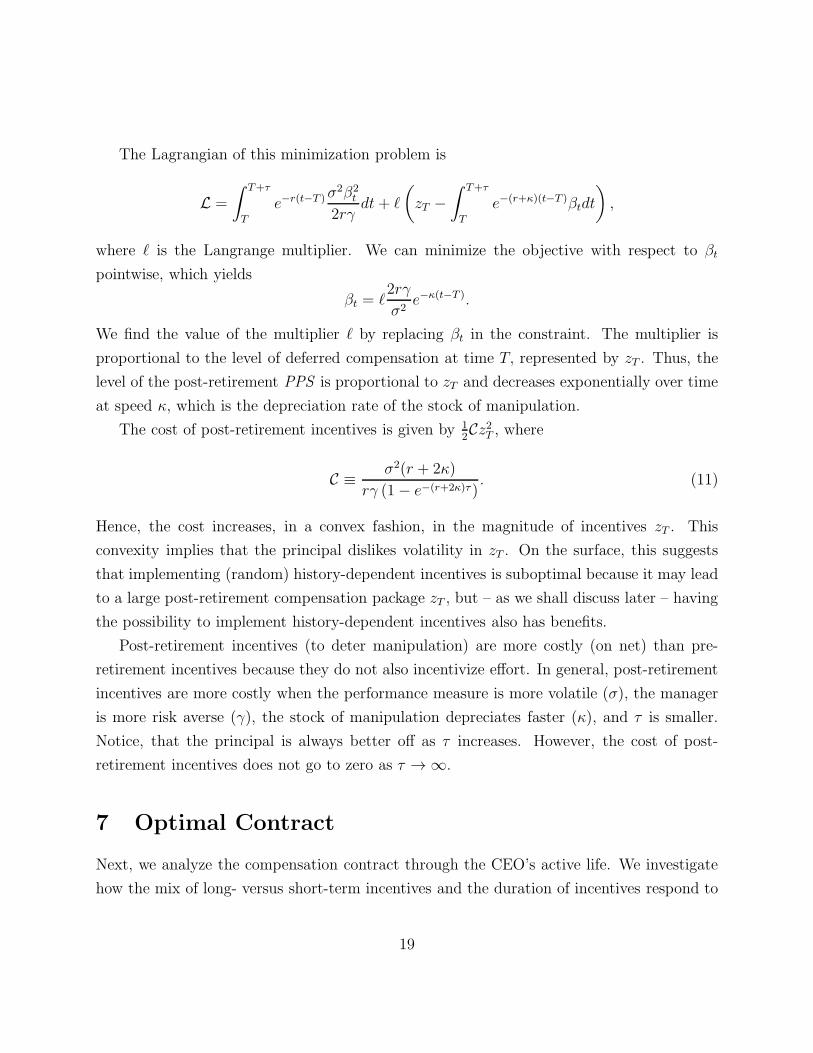
The Lagrangian of this minimization problem is

L =

∫ T+τ

T

e−r(t−T )σ2β2

t

2rγdt+ ℓ

(

zT −

∫ T+τ

T

e−(r+κ)(t−T )βtdt

)

,

where ℓ is the Langrange multiplier. We can minimize the objective with respect to βt

pointwise, which yields

βt = ℓ2rγ

σ2e−κ(t−T ).

We find the value of the multiplier ℓ by replacing βt in the constraint. The multiplier is

proportional to the level of deferred compensation at time T, represented by zT . Thus, the

level of the post-retirement PPS is proportional to zT and decreases exponentially over time

at speed κ, which is the depreciation rate of the stock of manipulation.

The cost of post-retirement incentives is given by 12Cz2T , where

C ≡σ2(r + 2κ)

rγ (1− e−(r+2κ)τ ). (11)

Hence, the cost increases, in a convex fashion, in the magnitude of incentives zT . This

convexity implies that the principal dislikes volatility in zT . On the surface, this suggests

that implementing (random) history-dependent incentives is suboptimal because it may lead

to a large post-retirement compensation package zT , but – as we shall discuss later – having

the possibility to implement history-dependent incentives also has benefits.

Post-retirement incentives (to deter manipulation) are more costly (on net) than pre-

retirement incentives because they do not also incentivize effort. In general, post-retirement

incentives are more costly when the performance measure is more volatile (σ), the manager

is more risk averse (γ), the stock of manipulation depreciates faster (κ), and τ is smaller.

Notice, that the principal is always better off as τ increases. However, the cost of post-

retirement incentives does not go to zero as τ → ∞.

7 Optimal Contract

Next, we analyze the compensation contract through the CEO’s active life. We investigate

how the mix of long- versus short-term incentives and the duration of incentives respond to

19

shocks throughout the CEO’s tenure.

Given the optimal post-retirement scheme derived previously, we can specialize the prin-

cipal problem in Lemma 1. Hereafter, it is convenient to eliminate manipulation as one of

the controls by noting that manipulation is given by5 mt = (at − φzt)+/g and defining the

payoff function as

π(a, z) ≡ a−λ

g(a− φz)+ −

1

2g

[

(a− φz)+]2

−(1 + rγσ2) a2

2.

We can rewrite the principal problem in Lemma 1 as

F (z, 0) = supz0,a,σz E[

∫ T

0e−rtπ(at, zt)dt− e−rT 1

2Cz2T

]

subject to

dzt = [(r + κ)zt + rγat(σσzt − 1)]dt+ σztdBt

(12)

The Hamilton–Jacobi–Bellman equation associated with problem (12) is as follows:6

rF = maxa,σz π(

a, z)

+ Ft + [(r + κ)z + rγa(σσz − 1)]Fz +12σ2zFzz

F (z, T ) = −12Cz2.

(13)

The terminal condition captures the cost of providing post-retirement incentives zt, as

derived in Section 6.1. Once we solve for the value function for arbitrary z0, we initialize the

contract at z0 = argmaxz F (z, 0).

Optimizing with respect to σz requires that the value function is concave. We can al-

ways ensure that the value function is weakly concave by introducing public randomization.

However, we have not been able to prove that the solution is strictly concave. Hereafter,

we assume that the value function is concave so that the following characterization applies

to regions of the state space where such randomization is not required. We have not found

instances in our examples where the use of randomization is required. Moreover, F (z, t) is

strictly concave in z at time T (because it satisfies the terminal condition), so F (z, t) is also

5We use the usual notation x+ ≡ max{x, 0}.6We omit the specification of the value function at the upper bound on zt as this is not needed for the

following analysis. We provide the specification of the boundary condition at the upper bound to the onlineappendix when we provide the numerical algorithm used for the solution of the HJB equation.

20

strictly concave for t close to T .7,8

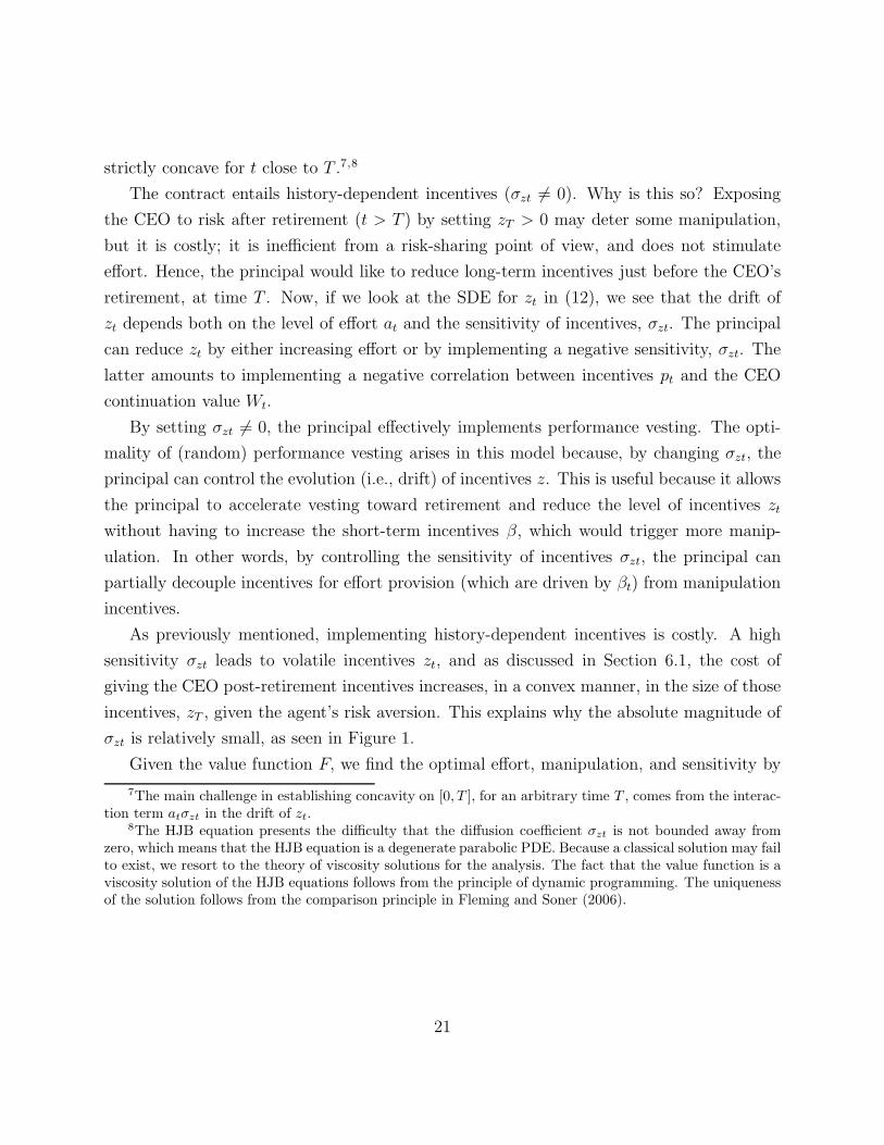
The contract entails history-dependent incentives (σzt 6= 0). Why is this so? Exposing

the CEO to risk after retirement (t > T ) by setting zT > 0 may deter some manipulation,

but it is costly; it is inefficient from a risk-sharing point of view, and does not stimulate

effort. Hence, the principal would like to reduce long-term incentives just before the CEO’s

retirement, at time T . Now, if we look at the SDE for zt in (12), we see that the drift of

zt depends both on the level of effort at and the sensitivity of incentives, σzt. The principal

can reduce zt by either increasing effort or by implementing a negative sensitivity, σzt. The

latter amounts to implementing a negative correlation between incentives pt and the CEO

continuation value Wt.

By setting σzt 6= 0, the principal effectively implements performance vesting. The opti-

mality of (random) performance vesting arises in this model because, by changing σzt, the

principal can control the evolution (i.e., drift) of incentives z. This is useful because it allows

the principal to accelerate vesting toward retirement and reduce the level of incentives zt

without having to increase the short-term incentives β, which would trigger more manip-

ulation. In other words, by controlling the sensitivity of incentives σzt, the principal can

partially decouple incentives for effort provision (which are driven by βt) from manipulation

incentives.

As previously mentioned, implementing history-dependent incentives is costly. A high

sensitivity σzt leads to volatile incentives zt, and as discussed in Section 6.1, the cost of

giving the CEO post-retirement incentives increases, in a convex manner, in the size of those

incentives, zT , given the agent’s risk aversion. This explains why the absolute magnitude of

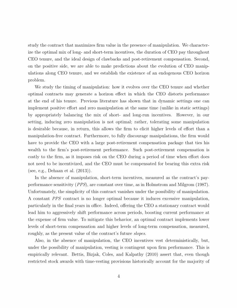
σzt is relatively small, as seen in Figure 1.

Given the value function F, we find the optimal effort, manipulation, and sensitivity by

7The main challenge in establishing concavity on [0, T ], for an arbitrary time T , comes from the interac-tion term atσzt in the drift of zt.

8The HJB equation presents the difficulty that the diffusion coefficient σzt is not bounded away fromzero, which means that the HJB equation is a degenerate parabolic PDE. Because a classical solution may failto exist, we resort to the theory of viscosity solutions for the analysis. The fact that the value function is aviscosity solution of the HJB equations follows from the principle of dynamic programming. The uniquenessof the solution follows from the comparison principle in Fleming and Soner (2006).

21

solving the optimization problem in the HJB equation. The optimal policy is then given by

a(z, t) = min{a(z, t), a}+ (14a)

a(z, t) =

g−λ+φz−rγgFz1+gH(Fz ,Fzz)

if 1− rγFz ≥ φzH(Fz, Fzz) +λg

1−rγFzH(Fz ,Fzz)

if 1− rγFz < φzH(Fz, Fzz)

φz otherwise

m(z, t) =1

g(a(z, t)− φz)+ (14b)

σz(z, t) = −rγσa(z, t)FzFzz

, (14c)

where H(Fz, Fzz) ≡ 1 + rγσ2 + r2γ2σ2(Fzz)−1F 2

z . The second-order condition requires that

1 + gH(Fz, Fzz) ≥ 0. σz(z, t) remains determined by (14c) if this condition is not satisfied.

However, the optimal effort now is either φz or a. In the particular case where g > λ, effort

is given by min(φz, a).

Due to its non-linearity, it is difficult to obtain analytical results by analyzing the HJB

equation (13) directly. However, we can derive some insights about the optimal contract

indirectly by analyzing the sample paths of the dual variable ψt = Fz(zt, t), which captures

the Principal’s marginal value of providing long-term incentives to the CEO. The approach

of analyzing the optimal contract by studying the sample paths of ψt follows the approach

used by Farhi and Werning (2013) and Sannikov (2014), and it is similar to the analysis

of deterministic contracts using optimal control developed in Section 8 (and the analogous

stochastic maximum principle). In fact, ψt is the stochastic analogue to the traditional

co-state variable in optimal control problems.

Because the payoff function π(a, z) fails to be differentiable at a = φz when λ > 0, we

assume that λ = 0 throughout the rest of this section. This assumption is required purely

for technical considerations and is not required when we solve the model numerically. Using

Ito’s Lemma and the Envelope Theorem, we derive the following representation for the dual

variable ψt, which is key in the characterization of the optimal contract. We find that the

22

pair (ψt, zt) solves the forward–backward stochastic differential equation

dψt = − (κψt + φmt) dt− rγσatψtdBt, ψ0 = 0,

dzt = [(r + κ)zt + rγat(σσzt − 1)]dt+ σztdBt, zT = −C−1ψT .

This means that, for any t ∈ [0, T ], the value of ψt is given by

ψt = −φ

∫ t

0

e−κ(t−s)Es,tmsds (15)

Es,t ≡ exp

{

−

∫ t

s

rγσaudBu −1

2

∫ t

s

r2γ2σ2a2udu

}

,

and hence ψt ≤ 0 for all t ∈ [0, T ]. Notice that ψt = 0 if and only if ms = 0 for all s < t. This

implies that σzt is zero (so incentives are deterministic) if there has been no manipulation

before time t.9 Equation (15) makes it possible to derive the qualitative properties of the

optimal contract and has the following implication: The marginal value of incentives has an

upper boundary at zero, and this implies that if the value function is concave, then there is

a lower bound z(t) for the long-term incentives; that is, zt ≥ z(t) where Fz(z(t), t) = 0. We

provide a qualitative characterization of the lower boundary z(t) in Proposition 3 and show

that this boundary decreases over time. This is consistent with the notion that the principal

wishes to reduce long-term incentives over time to avoid leaving the manager with a large

post-retirement package.

Furthermore, combining Equations (14c) and (15), we find that the sensitivity of incen-

tives is non-positive: positive shocks reduce the long-term incentive, reducing the duration of

incentives. This establishes the optimality of performance vesting discussed at the beginning

of this section. The following proposition records these results.

Proposition 3. If θ = r + κ, then the optimal contract has the following properties:

1. Lower bound on long-term incentives: There is a decreasing function z(t) ≥ 0 such

that zt ≥ z(t) for all t ∈ [0, T ], where z(T ) = 0 and z(t) > 0 for all t < T .

2. Long-term incentives and performance are negatively correlated: σzt ≤ 0 for all t ∈

[0, T ].

9We can show that this never happens if λ = 0, but the analysis of deterministic contracts suggests thatit could be the case if λ > 0.

23

3. Whenever mt > 0 the drift of long term incentives is negative, that is, Et(dzt) < 0.

Performance vesting is optimal (i.e., σzt < 0) because it provides an extra degree of

freedom to control the level of incentives zt without triggering excessive manipulation mt. In

contrast, under deterministic vesting, the only way to reduce the long-term incentives is by

increasing short-term incentives βt, which exacerbates manipulation and lowers the level of

effort the principal can implement in the future. This is precisely where performance vesting

helps: Long-term incentives can be reduced over-time without necessarily distorting the level

of effort. By adjusting the sensitivity of incentives σzt, the principal can control the drift of

zt while holding the trajectory of effort constant.

It is precisely the possibility of manipulation that justifies performance vesting in our

setting. On the surface, one might think that performance vesting exacerbates the CEO’s

incentive to manipulate since, by inflating performance, the CEO can accelerate vesting.

This logic is flawed. The manager’s manipulation incentive at a given point depends upon

the sensitivity of his continuation value to performance βt and duration zt, not upon the

sensitivity of duration σzt. Making vesting more or less sensitive to performance at time t,

by modifying σzt, does not affect the CEO manipulation incentives at time t. For example,

consider the case when βt = 0. The manager has no incentive to manipulate performance,

and this is true independent of the sensitivity of incentives σzt. In other words, as long as

βt does not change, the choice of σzt will not affect manipulation incentives at time t. Of

course, σzt has an indirect effect on incentives to manipulate in future periods due to its

effect on the duration of incentives (zt).

By setting a negative sensitivity σzt, the principal effectively implements a negative cor-

relation between pt andWt. Hence, positive shocks that boost the agent’s continuation value

Wt reduce the duration of incentives pt. In brief, good performance accelerates vesting.

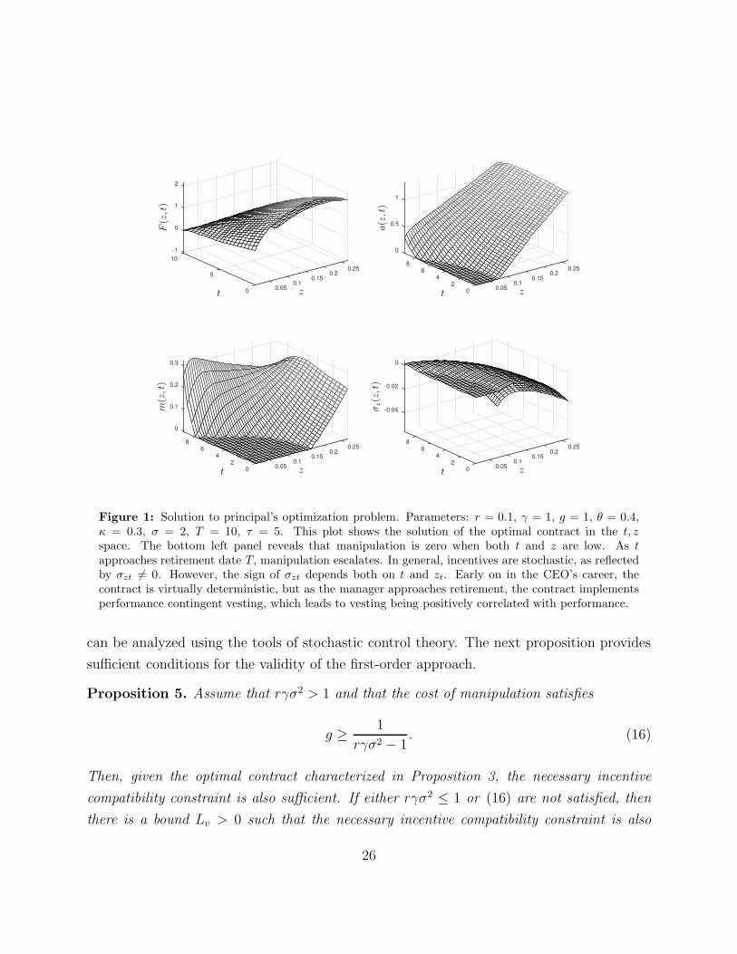
The evolution of zt resembles a mean-reverting process that follows a time-varying target

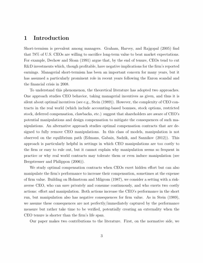
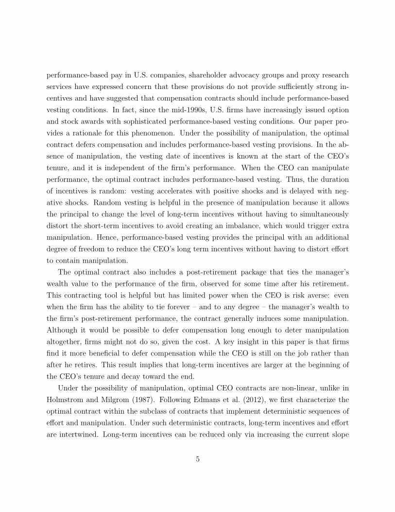
z(t) converging to zero as T becomes closer. Figure 2 shows the evolution of the lower

boundary z(t) together with the drift of zt. The lower bound decreases over time towards

zero, and the drift of z is negative above the lower bound on incentives, z(t). Moreover,

we show that whenever the optimal contract implements positive manipulation, the drift

of long-term incentives is negative. In particular, we have shown that the drift is negative

when zt is close to the lower boundary. 10 Long-term incentives revert toward the target z(t)

10We have not been able to sign the drift for values of zt such that mt = 0. However, we show that in the

24

over time, and the magnitude of the negative drift of zt increases when we are close to the

retirement date T . The relative importance of short-term incentives increases as the CEO

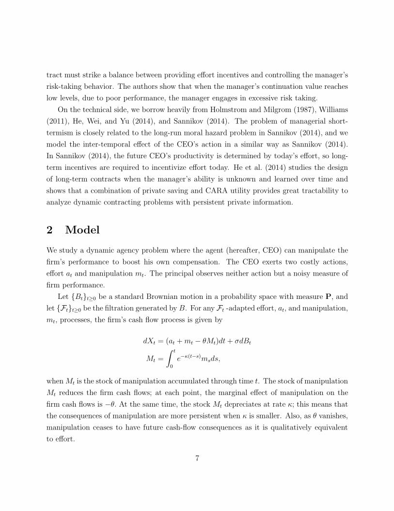
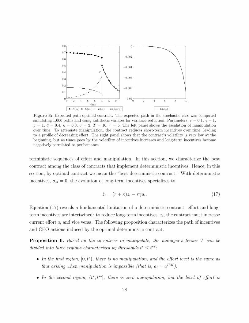
gets closer to retirement, explaining the CEO horizon effect. Figure 3 shows the evolution

of expected long-term incentives, effort, manipulation and sensitivity. Long-term incentives

and effort decrease, and manipulation increases over time. The volatility of incentives is low

at the beginning of tenure – so the contract’s evolution is close to deterministic; so that it

decreases over time (its absolute value increases). This means that the contract becomes

more sensitive to performance over time.

Consider the effect of enforcement on the optimal contract. Our model includes an upper

bound τ for the length of the clawback period [T, T + τ ]. This parameter captures the fact

that the principal cannot impose risk on the manager’s wealth forever, as this would be

impossible to enforce. It is not surprising then that a lower τ reduces the level of long-term

incentives. When the clawback period is shorter, providing long-term incentives towards

the end of the CEO’s tenure is more costly because it makes the CEO compensation more

risky. Moreover, a lower τ reduces the overall duration of CEO incentives. In fact, a lower

τ reduces the importance of long-term incentives at the beginning of the CEO’s tenure and

the lower bound on long-term incentives z(t), as the following proposition proves.

Proposition 4. If θ = r + κ, then

1. The lower boundary on long-term incentives, z(t), is increasing in τ .

2. Initial long-term incentive z0 are increasing in τ and T .

3. This implies that the initial effort is increasing in τ and T while the initial manipulation

is decreasing in both τ and T .

We conclude this section by revisiting the CEO’s problem and establishing sufficient

conditions for the validity of the first-order approach. This approach makes it possible to

find a recursive formulation for the principal problem and analyze the relaxed problem in

which we only consider the first-order conditions. Solving for the optimal contract is not

possible if the first-order approach is not valid because one lacks a recursive formulation that

case of contracts with deterministic vesting, that is σzt = 0, the drift of zt is always negative on the optimalpath.

25

-1

10

0

0.25

1

0.25

2

0.150.1

0.050

0

0.5

80.256

1

0.24 0.15

0.120.05

0

0

0.1

80.25

0.2

60.2

0.3

4 0.150.12

0.050

-0.04

80.25

-0.02

60.2

0

4 0.150.12

0.050 zz

zz

F(z,t)

m(z,t)

a(z,t)

σz(z,t)

tt

tt

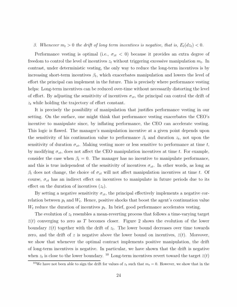
Figure 1: Solution to principal’s optimization problem. Parameters: r = 0.1, γ = 1, g = 1, θ = 0.4,κ = 0.3, σ = 2, T = 10, τ = 5. This plot shows the solution of the optimal contract in the t, z

space. The bottom left panel reveals that manipulation is zero when both t and z are low. As t

approaches retirement date T, manipulation escalates. In general, incentives are stochastic, as reflectedby σzt 6= 0. However, the sign of σzt depends both on t and zt. Early on in the CEO’s career, thecontract is virtually deterministic, but as the manager approaches retirement, the contract implementsperformance contingent vesting, which leads to vesting being positively correlated with performance.

can be analyzed using the tools of stochastic control theory. The next proposition provides

sufficient conditions for the validity of the first-order approach.

Proposition 5. Assume that rγσ2 > 1 and that the cost of manipulation satisfies

g ≥1

rγσ2 − 1. (16)

Then, given the optimal contract characterized in Proposition 3, the necessary incentive

compatibility constraint is also sufficient. If either rγσ2 ≤ 1 or (16) are not satisfied, then

there is a bound Lv > 0 such that the necessary incentive compatibility constraint is also

26

0 1 2 3 4 5 6 7 8 9

0

0.05

0.1

0.15

0.2

0.25

-0.035

-0.0

3

-0.03

-0.03

-0.03

-0.0

25

-0.025

-0.025

-0.025

-0.0

2

-0.02

-0.02

-0.0

15

-0.015

-0.015

-0.01

-0.01

-0.005

z z(t)

Tenure, tFigure 2: Lower bound (z(t)) and drift (Et(dzt)) of incentives. Parameters: r = 0.1, γ = 1, g = 1,θ = 0.4, κ = 0.3, σ = 2, T = 10, τ = 5. This plot shows the evolution of z(t) together with thedrift of the continuation value. The lower bound z(t) decreases over time towards zero, and the driftof zt is negative, which means that long-term incentives revert toward the target z(t). The black curverepresents z(t) while the contour lines represent the value of drift, Et(dzt), for different pairs (t, z).The relevant state space on-path corresponds to the the pairs (t, z) above the curve z(t), and a darkerbackground represents a lower (more negative) drift.

sufficient if −Lv ≤ σzt.

As in previous literature (He et al., 2014; Sannikov, 2014), the sufficiency of the first-

order approach requires that the sensitivity of long term incentives be bounded. However,

because in our setting this sensitivity is never positive, we only need to bound the sensitivity

from below. Moreover, when rγσ2 and g are high enough, the first-order approach is valid

for any non-positive sensitivity, and there is no need to impose any additional bound on

the sensitivity of incentives. Finally, notice that the first-order approach is always valid if

σzt = 0; so, the first order approach is always valid for the deterministic contracts considered

later in Section 8.

8 Deterministic Incentives

In general, effort and manipulation are history dependent; however, one can gain further

insights into the dynamics of compensation and CEO behavior by following Edmans et al.

(2012) and He et al. (2014) and looking at the subclass of contracts that implement de-

27

0 2 4 6 8 10 12 140

0.1

0.2

0.3

0.4

0.5

0.6

0.7

0.8

T

time

E(at) E(mt) E(zt) E(βt/rγ)

0 2 4 6 8 10−0.01

−0.008

−0.006

−0.004

−0.002

0

E(σzt)

Figure 3: Expected path optimal contract. The expected path in the stochastic case was computedsimulating 1,000 paths and using antithetic variates for variance reduction. Parameters: r = 0.1, γ = 1,g = 1, θ = 0.4, κ = 0.3, σ = 2, T = 10, τ = 5. The left panel shows the escalation of manipulationover time. To attenuate manipulation, the contract reduces short-term incentives over time, leadingto a profile of decreasing effort. The right panel shows that the contract’s volatility is very low at thebeginning, but as times goes by the volatility of incentives increases and long-term incentives becomenegatively correlated to performance.

terministic sequences of effort and manipulation. In this section, we characterize the best

contract among the class of contracts that implement deterministic incentives. Hence, in this

section, by optimal contract we mean the “best deterministic contract.” With deterministic

incentives, σzt = 0, the evolution of long-term incentives specializes to

zt = (r + κ)zt − rγat. (17)

Equation (17) reveals a fundamental limitation of a deterministic contract: effort and long-

term incentives are intertwined: to reduce long-term incentives, zt, the contract must increase

current effort at and vice versa. The following proposition characterizes the path of incentives

and CEO actions induced by the optimal deterministic contract.

Proposition 6. Based on the incentives to manipulate, the manager’s tenure T can be

divided into three regions characterized by thresholds t∗ ≤ t∗∗:

• In the first region, [0, t∗), there is no manipulation, and the effort level is the same as

that arising when manipulation is impossible (that is, at = aHM).

• In the second region, (t∗, t∗∗], there is zero manipulation, but the level of effort is

28

bounded by the magnitude of long-term incentives (at = φzt).

• In the third region, (t∗∗, T ], manipulation is positive and increasing over time.

• Depending on parameters, the regions (t∗, t∗∗] and (t∗∗, T ] can be empty.

Over time, long-term incentives zt are weakly decreasing while manipulation mt is weakly

increasing.

There are three distinct regions. In the first region, manipulation is not a concern. In the

second region, there is no manipulation, but preventing manipulation forces the principal to

lower the level of effort implemented. In the third region, preventing manipulation is too

costly: both effort and manipulation go up over time. The region (t∗∗, T ] is empty when

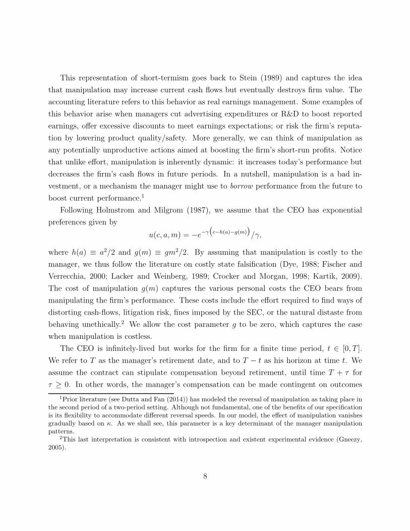
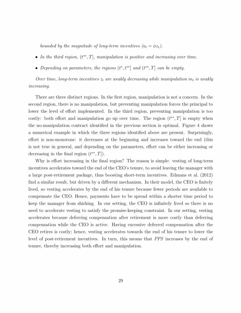
the no-manipulation contract identified in the previous section is optimal. Figure 4 shows

a numerical example in which the three regions identified above are present. Surprisingly,

effort is non-monotone: it decreases at the beginning and increases toward the end (this

is not true in general, and depending on the parameters, effort can be either increasing or

decreasing in the final region (t∗∗, T ]).

Why is effort increasing in the final region? The reason is simple: vesting of long-term

incentives accelerates toward the end of the CEO’s tenure, to avoid leaving the manager with

a large post-retirement package, thus boosting short-term incentives. Edmans et al. (2012)

find a similar result, but driven by a different mechanism. In their model, the CEO is finitely

lived, so vesting accelerates by the end of his tenure because fewer periods are available to

compensate the CEO. Hence, payments have to be spread within a shorter time period to

keep the manager from shirking. In our setting, the CEO is infinitely lived so there is no

need to accelerate vesting to satisfy the promise-keeping constraint. In our setting, vesting

accelerates because deferring compensation after retirement is more costly than deferring

compensation while the CEO is active. Having excessive deferred compensation after the

CEO retires is costly; hence, vesting accelerates towards the end of his tenure to lower the

level of post-retirement incentives. In turn, this means that PPS increases by the end of

tenure, thereby increasing both effort and manipulation.

29

0 2 4 6 8 100

0.05

0.1

0.15

0.2

0.25

0 2 4 6 8 100.1

0.2

0.3

0.4

0.5

0.6

t∗ t∗∗

time

Effort,Man

ipulation

Lon

gterm

incentives

at mtat mt zt

Figure 4: Parameters: r = 0.1, γ = 1, g = 1, θ = 0.5, κ = 0.3, σ = 2, T = 10, τ = 1. The deterministiccontract exhibits three regions. First, the CEO horizon is long enough such that manipulation is notan issue and effort is relatively high. Second, the contract implements zero manipulation but themanipulation constraint is binding, which leads to a decreasing effort profile.

The optimal contract induces manipulation sometimes, but not necessarily in every in-

stant of the manager’s tenure. As mentioned above, the CEO’s tenure consists of three

phases, ranked by the intensity of manipulation. During the first phase, manipulation in-

centives are weak because the CEO horizon is long, which means the principal has enough

time to “detect” and penalize the manager’s manipulation. As a consequence, short-run

incentives are strong and the manager exerts high effort and zero manipulation. During

the second phase, the manager’s manipulation incentives are binding, but the contract still

implements zero manipulation. However, to prevent manipulation, the principal is forced to

distort the contract PPS downward, which leads to a pattern of decreasing effort. During the

third phase, vesting speeds up, manipulation incentives become stronger, and manipulation

escalates.

Long-term incentives have to mature over time, as the manager approaches retirement,

and this process tilts incentives toward the short run. In turn, this triggers manipulation,

but may also boost effort in the final years. We can think of these two effects as mirror

images: providing high post-retirement compensation is costly. To reduce it, some of the

contract’s long-term incentives must mature, which in turn increases short-term incentives.

The relative length of the three phases in the manager’s tenure depends on the severity of the

30

manipulation problem. Thus, for instance, when the reversal of manipulation is slow (low

θ), enforcement is weak (low τ), or manipulation is easy (low g), the relative importance of

the third phase grows at the expense of the other two phases, especially the first one.

We find that the optimal contract follows similar patterns to the ones in the contract with

deterministic vesting. In the next section, we discuss the predictions of the model and provide

some numerical examples and comparative statics. In most of our examples, the long-term

incentive sensitivity implemented by the stochastic contract – which is itself random – is very

small on average. Hence, the deterministic contract seems like a good approximation of the

state-contingent contract, and it captures the evolution of CEO behavior and incentive-pay

very accurately, particularly at the beginning of CEO’s tenure.

9 The Model at Work: Numerical Examples and Em-

pirical Implications

In this section, we discuss the empirical implications of the model and relate them to existing

evidence.

Vesting and short-termism With regard to short-termism and vesting, Edmans et al.

(2013) show that CEO manipulations increase during years with significant amounts of shares

and option vesting. The authors find that, in years in which the CEOs experience signif-

icant equity vesting, they cut investments in R&D, advertising, and capital expenditures.

Seemingly, vesting induces CEOs to act myopically in order to meet short-term targets.

Horizon, Short-Termism, and Pay Duration. The executive compensation literature

hypothesizes the existence of a “CEO Horizon problem” whereby CEO short-termism would

be particularly severe in the final years of CEO office, in so far as the manager is unable to

internalize the consequences of his actions. Gibbons and Murphy (1992) indeed hypothesize

that existing compensation policies induce executives to reduce investments during their last

years of office but do not find conclusive evidence of greater manipulation. Gonzalez-Uribe

and Groen-Xu (2015) find that “CEOs with more years remaining in their contract pursue

more influential, broad and varied innovations.” Dechow and Sloan (1991) document that

31

managers tend to reduce R&D expenditures as they approach retirement, and the reductions

in R&D are mitigated by CEO stock ownership.

Although intuitive, the CEO horizon hypothesis seems to ignore the fact that manager

incentives are endogenous. If shareholders anticipate the CEO horizon problem, arguably

they will adjust compensation contracts accordingly. This could explain why the empirical

evidence regarding the relation between manipulation and tenure is ambivalent (Gibbons and

Murphy (1992)). Cheng (2004), for instance finds that compensation contracts become par-

ticularly insensitive to accounting performance measures that are easily manipulable by the

end of the manager’s tenure, suggesting that compensation committees are able to anticipate

the manager’s incentives. In this paper, we show that a CEO horizon problem exists even in

the presence of endogenous incentives. The finite nature of CEO’s tenure and the fact that

deferring compensation after retirement is costly, explain why optimal contracts implement

manipulation in our setting. In Section 5, we show that when the manager horizon grows

large (T → ∞), the possibility of manipulation is irrelevant. Linear contracts such as the

one analyzed by Holmstrom and Milgrom (1987) suffice to eliminate manipulation. This

result is consistent with Jensen (2001, 2003), who recommends linear contracts to prevent

managers from gaming compensation systems. In sum, our analysis suggests that when the

CEO has a limited horizon, linear contracts are unable to prevent short-termism and may

even induce too much.11

From a contracting perspective, two tools are effective at dealing with the possibility of

manipulations: i) deferred compensation and ii) clawbacks. Both tools are used in practice.

Some empirical evidence suggests that after SOX the average duration of CEO compensa-

tion increased, and firms started to rely more on restricted stock to compensate managers.

Gopalan et al. (2014) provide evidence that the duration of stock-based compensation is

about three to five years. They document a negative association between the duration of

incentives and measures of manipulation such as discretionary accruals. In particular, they

find that this duration is shorter for older executives and those with longer tenures. The

second instrument is clawbacks. A clawback is a contractual clause included in employment

contracts whereby the manager is obliged to return previously awarded compensation due

to special circumstances, which are described in the contract, for example a fraud or re-

11Kothari and Sloan (1992) provides evidence that accounting earnings commonly take up to three yearsto reflect changes in firm value

32

statement. The growing popularity of clawback provisions is due, at least in part, to the

Sarbanes–Oxley Act of 2002, which requires the U.S. Securities and Exchange Commission

(SEC) to pursue the repayment of incentive compensation from senior executives who are

involved in a fraud or a restatement.12 Although we do not incorporate clawbacks – as a

discrete event triggered by a restatement – in our model, the fact that the manager’s income

depends on post-retirement performance captures the essence of clawbacks as an incentive

mechanism.

Pay-for-Performance The executive compensation literature has documented at least

two puzzles regarding pay-performance sensitivity. First, pay for performance evolves with

CEO tenure (Brickley et al. (1999)). Unlike in Holmstrom and Milgrom (1987), a constant

PPS is not optimal in our setting. Indeed, a constant PPS would lead to excessive manip-

ulation, especially around the retirement date. Our model predicts a profile of increasing

manipulation along with a relatively low but potentially increasing PPS. Some evidence sug-

gests that the PPS of CEO compensation increases over time, as manager’s stock ownership

grows (Gibbons and Murphy (1992)). At first blush, this fact seems to contradict the predic-

tions of our model. In our setting, PPS may increase over time; however, it is never higher

than at the start of tenure, and it is non-monotonic in time; it only increases at the end. A

time profile of increasing PPS is consistent with an extended version of the model in which

the performance measure is a distorted version of the firm’s cash flows (for example, the

firm earnings). A second empirical puzzle that was identified in the 1990s is the low PPS in

CEO contracts (see e.g., Jensen (2001)). Our model predicts that such low PPS could be

the result of the possibility of manipulation, as already suggested by Goldman and Slezak

(2006).

Corporate Governance and Short-Termism The CEO horizon problem is ultimately

a corporate governance weakness reflecting the inability of the firm to monitor the CEO’s

actions. If we understand corporate governance as a set of mechanisms (some of which are

exogenous to the firm) that make it more costly for the manager to manipulate performance

(for example, by increasing the cost of manipulation g), then our model predicts that better

12The prevalence of clawback provisions among Fortune 100 companies increased from less than 3% priorto 2005 to 82% in 2010.

33

corporate governance would result in higher short-term compensation (lower duration) and

greater firm value. Maybe paradoxically, it does not predict that the levels of manipulation

will be lower. If better corporate governance makes short-run incentives relatively more

effective at stimulating effort, vis-a-vis manipulation, then the firm may find it optimal to

offer stronger short-term incentives, even at the expense of tolerating greater manipulations.

This effect is present in previous static models of costly state falsification. For example,

Lacker and Weinberg (1989) show that no manipulation is optimal when the cost of manip-

ulation is not overly convex. In our setting, with a quadratic falsification cost, this condition

translates into a low value of g. From the IC constraint, we find that the sensitivity of ma-

nipulation to changes in effort (for a fixed z) is 1/rγg. This means that when the marginal

cost of manipulation g is low, the trade-off between higher effort and higher manipulation

is too high. A small increment in effort generates so much manipulation that it makes the

no-manipulation optimal. In fact, when g = 0, the optimal contract implements no manip-

ulation. Hence, in this case, the optimal contract implements no manipulation. Of course

one needs to be careful when interpreting this observation as evidence that short-run incen-

tives cause manipulation (Bergstresser and Philippon (2006)). As the cost of manipulation

g grows large, the manager’s manipulation incentives are vanishingly low. The contract then

becomes stationary – with constant PPS – because short-term incentives suffice to induce

effort.

Another parameter that relates to corporate governance is τ . Recall that τ captures the

length of the clawback period; namely, how long after retirement principal the principal can

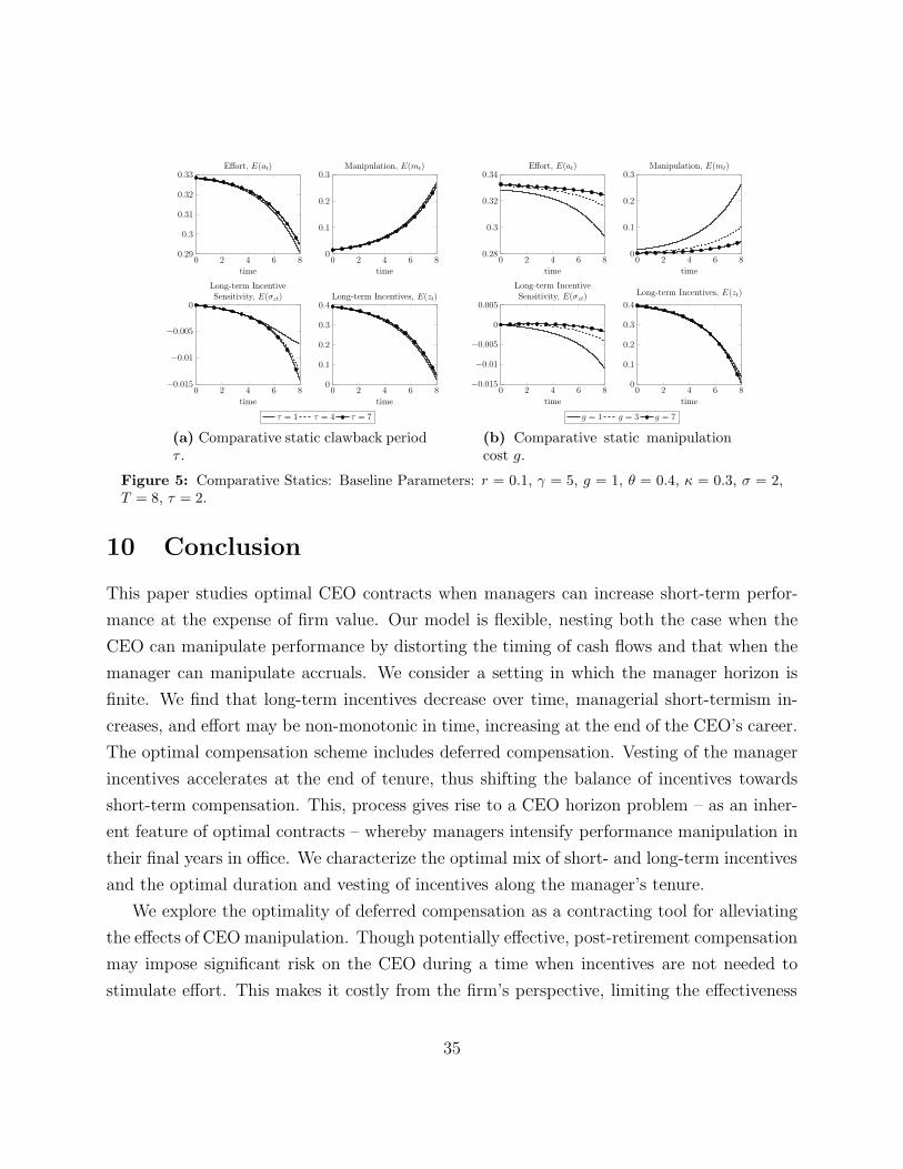
tie the CEO’s wealth to the firm’s performance. Figure 5a shows that a longer clawback

period allows the principal to induce higher effort and less manipulation. The contract tends

to rely more on performance-contingent vesting, and long-term incentives tend to be higher.

As mentioned previously, extending τ is not a panacea. The consequences of manipulation

are present even as τ grows large because providing a large post-retirement package over

a long clawback period can eliminate manipulation, although, as a downside, this would

impose excessive risk on the manager.

34

0 2 4 6 80.29

0.3

0.31

0.32

0.33

time

Effort, E(at)

τ = 1 τ = 4 τ = 7

0 2 4 6 80

0.1

0.2

0.3

time

Manipulation, E(mt)

0 2 4 6 8−0.015

−0.01

−0.005

0

time

Long-term IncentiveSensitivity, E(σzt)

0 2 4 6 80

0.1

0.2

0.3

0.4

time

Long-term Incentives, E(zt)

(a) Comparative static clawback periodτ .

0 2 4 6 80.28

0.3

0.32

0.34

time

Effort, E(at)

0 2 4 6 80

0.1

0.2

0.3

time

Manipulation, E(mt)

0 2 4 6 8−0.015

−0.01

−0.005

0

0.005

time

Long-term IncentiveSensitivity, E(σzt)

g = 1 g = 3 g = 7

0 2 4 6 80

0.1

0.2

0.3

0.4

time

Long-term Incentives, E(zt)

(b) Comparative static manipulationcost g.

Figure 5: Comparative Statics: Baseline Parameters: r = 0.1, γ = 5, g = 1, θ = 0.4, κ = 0.3, σ = 2,T = 8, τ = 2.

10 Conclusion

This paper studies optimal CEO contracts when managers can increase short-term perfor-

mance at the expense of firm value. Our model is flexible, nesting both the case when the

CEO can manipulate performance by distorting the timing of cash flows and that when the

manager can manipulate accruals. We consider a setting in which the manager horizon is

finite. We find that long-term incentives decrease over time, managerial short-termism in-

creases, and effort may be non-monotonic in time, increasing at the end of the CEO’s career.

The optimal compensation scheme includes deferred compensation. Vesting of the manager

incentives accelerates at the end of tenure, thus shifting the balance of incentives towards

short-term compensation. This, process gives rise to a CEO horizon problem – as an inher-

ent feature of optimal contracts – whereby managers intensify performance manipulation in

their final years in office. We characterize the optimal mix of short- and long-term incentives

and the optimal duration and vesting of incentives along the manager’s tenure.

We explore the optimality of deferred compensation as a contracting tool for alleviating

the effects of CEO manipulation. Though potentially effective, post-retirement compensation

may impose significant risk on the CEO during a time when incentives are not needed to

stimulate effort. This makes it costly from the firm’s perspective, limiting the effectiveness

35

of such compensation.

Unlike in Holmstrom and Milgrom (1987), the optimal contract is non-linear in perfor-

mance. Moreover, it implements path-dependent effort and manipulation, effectively making

the firm’s performance more noisy. Under a deterministic contract, the firm can modify the

long-term incentives only by distorting the CEO’s effort (for the contract to preserve in-

centive compatibility). History-dependent incentives help because they allow the firm to

control the evolution of long-term incentives without exacerbating manipulations. The op-

timal contract is one in which the sensitivity of long-term incentives to firm performance at

the beginning of the CEO’s tenure and at the end are qualitatively different. At the begin-

ning, positive performance shocks increase the use of long-term incentives; in other words,

the duration of incentives increases when the firm is performing well. On the contrary, at

the end of the CEO’s tenure, long-term incentives are negatively correlated to the firm’s

performance. Positive performance shocks lead to an acceleration of incentive vesting.

We conclude by noting that the design of monetary incentives alone is not enough to

eliminate managerial short-termism. In practice, other corporate governance tools may com-

plement the disciplining role of compensation. For example, we can presume that CEOs’

discretion to make short-term investments or cut long-term ones evolves over time, being a

function of the manager’s horizon. There are different ways in which this could be addressed.

For example, the level of discretion a CEO receives affects the freedom he has to manipulate

performance, but it also makes him less productive. In other words, the CEO might not

be able to manipulate performance as freely as before, and the associated lack of flexibility

could also reduce his productivity. Specifically, assume that under low discretion the man-

ager’s effort only produces a fraction of what it produces otherwise (that is, the marginal

productivity of effort is αat for some α < 1). Our analysis suggests that CEOs should be

given more discretion at the beginning of their tenures, with an increment in board oversight

taking place as he gets close to retirement. Of course, this policy recommendation must be

taken with a grain of salt. There are additional factors that we have ignored in the model.

One of these factors is learning; a young and inexperienced CEO’s talent may be uncertain,

and the board may want to monitor his actions more closely.

36

References

Baker, G. P. 1992. Incentive contracts and performance measurement. Journal of Political

Economy 100(3):598–614.

Barles, G and P. E. Souganidis. 1991. Convergence of approximation schemes for fully

nonlinear second order equations. Asymptotic analysis 4(3):271–283.

Bergstresser, D and T. Philippon. 2006. CEO incentives and earnings management. Journal

of Financial Economics 80(3):511–529.

Bettis, C, J. Bizjak, J. Coles. and S. Kalpathy. 2010. Stock and option grants with

performance-based vesting provisions. Review of Financial Studies :hhq060.

Beyer, A, I. Guttman. and I. Marinovic. 2014. Optimal contracts with performance manip-

ulation. Journal of Accounting Research 52(4):817–847.

Brickley, J. A, J. S. Linck. and J. L. Coles. 1999. What happens to ceos after they retire? new

evidence on career concerns, horizon problems, and ceo incentives. Journal of Financial

Economics 52(3):341–377.

Cheng, S. 2004. R&d expenditures and ceo compensation. The Accounting Review 79(2):305–

328.

Crandall, M. G, H. Ishii. and P.-L. Lions. 1992. User’s guide to viscosity solutions of sec-

ond order partial differential equations. Bulletin of the American Mathematical Soci-

ety 27(1):1–67.

Crocker, K. J and J. Morgan. 1998. Is honesty the best policy? curtailing insurance fraud

through optimal incentive contracts. Journal of Political Economy 106(2):355–375.

Crocker, K. J and J. Slemrod. 2007. The economics of earnings manipulation and managerial

compensation. The RAND Journal of Economics 38(3):698–713.

Cziraki, P and M. Xu. 2014. Ceo job security and risk-taking. Technical report, London

School of Economics.

37

Dechow, P. M and R. G. Sloan. 1991. Executive incentives and the horizon problem: An

empirical investigation. Journal of Accounting and Economics 14(1):51–89.

Dehaan, E, F. Hodge. and T. Shevlin. 2013. Does voluntary adoption of a clawback provision

improve financial reporting quality? Contemporary Accounting Research 30(3):1027–1062.

DeMarzo, P. M, D. Livdan. and A. Tchistyi. 2013. Risking other people’s money: Gambling,

limited liability, and optimal incentives.

Dutta, S and Q. Fan. 2014. Equilibrium earnings management and managerial compensation

in a multiperiod agency setting. Review of Accounting Studies 19(3):1047–1077.

Dye, R. A. 1988. Earnings management in an overlapping generations model. Journal of

Accounting Research:195–235.

Edmans, A, V. W. Fang. and K. A. Lewellen. 2013. Equity vesting and managerial myopia.

Technical report, National Bureau of Economic Research.

Edmans, A, X. Gabaix, T. Sadzik. and Y. Sannikov. 2012. Dynamic CEO compensation.

Journal of Finance 67(5):1603–1647.

Farhi, E and I. Werning. 2013. Insurance and taxation over the life cycle. The Review of

Economic Studies 80(2):596–635.

Fischer, P. E and R. E. Verrecchia. 2000. Reporting bias. The Accounting Review 75(2):229–

245.

Fleming, W. H and H. M. Soner. 2006. Controlled Markov Processes and Viscosity Solutions,

Volume 25. Springer.

Forsyth, P. A and K. R. Vetzal. 2012. Numerical methods for nonlinear pdes in finance. In

Handbook of Computational Finance, pp. 503–528. Springer.

Gibbons, R and K. J. Murphy. 1992. Does executive compensation affect investment? NBER

Working Paper (w4135).

Gneezy, U. 2005. Deception: The role of consequences. The American Economic Re-

view 95(1):384–394.

38

Goldman, E and S. L. Slezak. 2006. An equilibrium model of incentive contracts in the

presence of information manipulation. Journal of Financial Economics 80(3):603–626.

Gonzalez-Uribe, J and M. Groen-Xu. 2015. Ceo contract horizon and innovation. Available

at SSRN 2633763 .

Gopalan, R, T. Milbourn, F. Song. and A. V. Thakor. 2014. Duration of executive compen-

sation. Journal of Finance 69(6):2777–2817.

Graham, J. R, C. R. Harvey. and S. Rajgopal. 2005. The economic implications of corporate

financial reporting. Journal of Accounting and Economics 40(1):3–73.

Guttman, I, O. Kadan. and E. Kandel. 2006. A rational expectations theory of kinks in

financial reporting. The Accounting Review 81(4):811–848.

He, Z, B. Wei. and J. Yu. 2014. Optimal long-term contracting with learning. Review of

Financial Studies 30(6):2006–2065.

Holmstrom, B and P. Milgrom. 1987. Aggregation and linearity in the provision of intertem-

poral incentives. Econometrica:303–328.

Jensen, M. C. 2001. Budgeting is broken - let’s fix it. Harvard Business Review 79(10):94–

101.

———. 2003. Paying people to lie: The truth about the budgeting process. European

Financial Management 9(3):379–406.

Kartik, N. 2009. Strategic communication with lying costs. The Review of Economic Stud-

ies 76(4):1359–1395.

Kartik, N, M. Ottaviani. and F. Squintani. 2007. Credulity, lies, and costly talk. Journal of

Economic theory 134(1):93–116.

Katzourakis, N. 2014. An Introduction to Viscosity Solutions for Fully Nonlinear PDE with

Applications to Calculus of Variations in L∞. Springer.

39

Kothari, S. P and R. G. Sloan. 1992. Information in prices about future earnings: Implica-

tions for earnings response coefficients. Journal of Accounting and Economics 15(2):143–

171.

Kushner, H and P. G. Dupuis. 2013. Numerical Methods for Stochastic Control Problems in

Continuous Time, Volume 24. Springer.

Lacker, J. M and J. A. Weinberg. 1989. Optimal contracts under costly state falsification.

The Journal of Political Economy :1345–1363.

Ma, J and J. Yong. 1999. Forward-Backward Stochastic Differential Equations and their

Applications. Number 1702. Springer.

Maggi, G and A. Rodriguez-Clare. 1995. Costly distortion of information in agency problems.

The RAND Journal of Economics :675–689.

Narayanan, M. 1985. Managerial incentives for short-term results. Journal of Fi-

nance 40(5):1469–1484.

Peng, L and A. Roell. 2014. Managerial incentives and stock price manipulation. The Journal

of Finance 69(2):487–526.

Pham, H. 2009. Continuous-Time Stochastic Control and Optimization with Financial Ap-

plications, Volume 61. Springer.

Protter, P. E. 1990. Stochastic Integration and Differential Equations (Second ed.). Springer.

Sabac, F. 2008. Dynamic incentives and retirement. Journal of Acccounting and Eco-

nomics 46(1).

Sannikov, Y. 2014. Moral hazard and long-run incentives. Technical report, mimeo, Princeton

University.

Stein, J. C. 1989. Efficient capital markets, inefficient firms: A model of myopic corporate

behavior. The Quarterly Journal of Economics :655–669.

Tourin, A. 2013. Introduction to finite differences methods. In Optimal Stochastic Control,

Stochastic Target Problems, and Backward SDE, pp. 201–212. New York, NY: Springer.

40

Varas, F. forthcoming. Managerial short-termism, turnover policy, and the dynamics of

incentives. Review of Financial Studies .

Williams, N. 2011. Persistent private information. Econometrica 79(4):1233–1275.

Yong, J and X. Y. Zhou. 1999. Stochastic Controls: Hamiltonian Systems and HJB equations,

Volume 43. Springer.

Zhu, J. Y. 2018. Myopic agency. Review of Economic Studies 85:1352–1388.

41

Appendix

A Necessary Conditions Incentive Compatibility

First we analyze the CEO’s optimization problem in (19) and derive the conditions stated

in Proposition 1. Given a contract prescribing actions (ct, at, mt), and any CEO strategy

(c, a, m), we denote a deviation from the contract’s recommended actions by ∆c ≡ c − c,

∆a ≡ a − a and ∆m ≡ m − m. We simplify the notation by denoting the CEO’s utility

flow if he follows the contract’s recommendation by ut ≡ u(ct, at, mt) and by u∆t ≡ u(ct +

∆ct, at +∆at, mt +∆mt) if he deviates.

A contract is a function of the entire performance path Xt, which makes the analysis of

the CEO’s problem involved. To overcome this challenge, we follow the approach proposed

by Williams (2011) and introduce the following change of measure. Let P be the probability

measure under recommendation {(a,m)}t∈[0,T ] and let P∆ be the probability measure induced

by the deviation {(a, m)}t∈[0,T ]. For any such deviation, we define the exponential martingale:

ξt ≡ exp

(

−1

2

∫ t

0

η2sds+

∫ t

0

ηsdBs

)

ηt ≡1

σ(∆at +∆mt − θ∆Mt).

By Girsanov’s theorem, the Radon-Nikodym derivative between P∆ and P is given by

dP∆/dP = ξT+τ . Using the fact that E (ξT+τ | Ft) = ξt and the law of iterated expectations,

we can write the CEO’s expected payoff given a deviation as

U(c, a, m) = E(a,m)

[∫ T+τ

0

e−rtξtu∆t dt + e−r(T+τ)ξT+τ

u∆T+τr

]

. (18)

The change of variables in equation (18) is useful because it allows to fix the expectation

operator by introducing the new state variable ξt in the CEO’s optimization problem. Under

this change of variables the agent problem is a stochastic control problem with random

coefficients (Williams (2011)).

Notice that, without loss of generality, we can take the recommendation (ct, at, mt) as a

reference point and consider the optimization with respect to (∆ct,∆at,∆mt). A contract is

42

incentive compatible if and only if ∆c = ∆a = ∆m = 0 is the CEO’s optimal choice. Using

equation (18), we can write the CEO’s problem as

sup∆c,∆a,∆mU(c+∆c, a +∆a,m+∆m)

subject to

dξt = − ξtσ(∆at +∆mt − θ∆Mt)dBt

d∆Mt = (∆mt − κ∆Mt)dt

dSt = (rSt −∆ct)dt.

(19)

As mentioned above, this is a stochastic control problem which can be can analyzed using

the stochastic maximum principle – a generalization of Pontryagin’s maximum principle to

stochastic control problems (Yong and Zhou, 1999).

We begin by defining the (current value) Hamiltonian function H as follows:

H = ξu∆ + qM(∆m− κ∆M) + qS(rS −∆c)− νξξ

σ(∆a +∆m− θ∆M), (20)

There are three control variables (∆a,∆m,∆c) three state variables (∆M,S, ξ) and their

associated adjoint variables (qM ,qS, qξ). The first two state variables (∆M,S) have drift but

are not (directly) sensitive to cash flow shocks. The third state variable ξ is a martingale;

its sensitivity to shocks is νξ.

We maximize the Hamiltonian with respect to the control variables. Because the Hamil-

tonian is jointly concave in (∆c,∆a,∆m), it suffices to consider the first order conditions

evaluated at ∆a = ∆m = ∆c = 0. This yields the following first order conditions:

uat =νξtσ

umt =νξtσ

− qMt uct = qSt

along with the complementary slackness conditions for the non-negativity constraint of mt.

The three adjoint variables (qSt , qMt , q

ξt ) follow stochastic differential equations which are the

43

stochastic analogue of the differential equations in optimal control theory:

dqSt = rqSt dt−∂Ht

∂Stdt+ νSt dBt = νSt dBt

dqMt = rqMt dt−∂Ht

∂∆Mt

dt+ νMt dBt =

(

(r + κ)qMt + θνξtσ

)

dt+ νMt dBt

dqξt = rqξt dt−∂Ht

∂ξtdt+ νξt dBt = (rqξt − ut)dt+ νξt dBt.

The adjoint equations must satisfy the transversality conditions qξT+τ =uT+τ

r, qMT+τ = 0 and

qST+τ =uc,T+τ

r. Theses equations are standard in stochastic control theory, but their economic

meaning will become clear later.

First, we solve for qξt by integrating its SDE and using the corresponding transversality

condition, which yields

qξt = Et

[∫ T+τ

t

e−r(s−t)usds+ e−r(T+τ)uT+τr

]

.

It’s now apparent that the adjoint variable qξt captures the evolution of the CEO’s contin-

uation value, so we follow the standard notation in the contracting literature and denote

Wt = qξt . It is also convenient to write the sensitivity of the continuation value to cash flow

shocks as νξt ≡ −βtWtσ. The SDE of the continuation value can thus be rewritten as

dWt = (rWt − ut)dt− βtWtσdBt. (21)

βt thus captures the sensitivity of Wt to shocks dBt (recall that Wt is negative, given the

negative exponential utility). βt is often referred to as the pay-performance-sensitivity.13

Hereafter, we refer to βt as the CEO’s short-run incentives or PPS.

We arrive at equation (5a) by plugging the private savings condition (6) in the above

equation. Equation (5b), on the other hand, is derived from the stochastic differential

equation for the adjoint variable of manipulation, qMt . Specifically, pt ≡ qMt /θ captures the

contract’s long-term incentives and measures the incentive power of deferred compensation

13In the case of contracts implementing a deterministic sequence of effort and manipulation, βt is propor-tional to the sensitivity of consumption to cash-flows that corresponds to the traditional definition of PPSin the empirical literature adapted to our setting.

44

to deter manipulation.

Finally, we study the CEO’s saving strategy. Using the first order condition for consump-

tion uc = qS and the stochastic differential equation for the adjoint variable qSt , we conclude

that the marginal utility of consumption follows the following stochastic differential equation:

duct = νSt σdBt. (22)

Equation (22) is the continuous-time version of the classic Euler equation for consumption,

which states that the marginal utility of consumption must be a martingale when the CEO’s

discount rate is equal to the market’s interest rate, or else the CEO would save or borrow

money to smooth-out his consumption path.

We find equation (22) by using a guess and verify approach. As in He et al. (2014), we

conjecture that Wt = rut, and given the CARA utility, we find that uc = −γu = −γrW .

Replacing this relation into equation (22) and setting νSt = rγβtWtσ, we obtain that

duct = −rγdWt = rγβtWtσdBt. (23)

Dividing by −rγ we find that equation (23) coincides with equation (21) and verify that

uct = −rγWt solves the adjoint equation for qSt . Hence, the marginal utility of consumption

uc and the continuation utility Wt are martingales. This result, due to He et al. (2014),

combines two observations. First, the CEO can smooth consumption inter-temporally, so

his marginal utility of consumption is a martingale. Second, under CARA preferences, the

CEO’s continuation value Wt is linear in flow utility ut.

The first order conditions along with the private savings condition, u = rW, yield the

necessary incentive conditions for effort and manipulation stated in Proposition 1:

rγh′(at) = βt (24a)

rγg′(mt) = βt + θptWt

, (24b)

The complementary slackness condition equation (5a) is obtained by replacing ut = rWt into

equation (21) and defining νMt ≡ σptWtσ.

45

B Sufficiency Agent Incentive Compatibility

To prove sufficiency, we follow Sannikov (2014) and He et al. (2014) in the construction of

an upper bound for the payoff after a deviation. In particular, we construct an upper bound

of the form

Wt = Wte−rγ(St+L1∆M2

t )+θzt∆Mt.

Let P∆ be the measure induced by a deviation (∆at,∆mt)t∈[0,T ] and let

B∆t ≡ Bt −

∫ t

0

(∆as +∆ms − θ∆Ms)

σds.

By Girsanov’s theorem, B∆t is a Brownian motion under P∆, which means that under P∆

dWt = −βtWt(∆at +∆mt − θ∆Mt)dt− βtWtσdB∆t

dzt =[

(r + κ)zt + βt(σσzt − 1) + σztσ(∆at +∆mt − θ∆Mt)

]

dt+ σztdB∆t

WT+τ =uR(cT+τ )

r

zT+τ = 0

Using Ito’s Lemma we find that

dWt = Wt(µWt dt+ σWt dB

∆t )

where

µWt =− rγ(rSt −∆ct) + 2rγκL1∆M2t − rγ(−φzt + 2L1∆Mt)∆mt +

1

2r2γ2φ2∆M2

t σ2zt

+ rγφ∆Mt[rzt + βt(σσzt − 1)] + rγφ∆Mtσztσ

(∆at +∆mt − θ∆Mt)

− rγat(∆at +∆mt − θ∆Mt)− rγφσβt∆Mtσzt.

Let W∆t be the expected payoff given the deviation (∆at,∆mt,∆ct)t∈[0,T+τ ]. For any

fixed t0 and t ∈ [t0, T + τ ], define the process

Gt0,t ≡

∫ t

t0

e−r(s−t0)u∆s ds+ e−r(t−t0)Wt,

46

where

u∆t ≡ u(

ct +∆ct, (at +∆at)1t≤T , (mt +∆mt)1t≤T)

,

and notice that by definition E[Gt0,T+τ ] =W∆t . Differentiating Gt0,t we get

ertdGt0,t = u∆t − rWtdt− rγµWt Wtdt+ σWt WtdBt.

Using the first order condition for the agent’s consumption, rWt = ut ≡ u(ct, at1t<T , mt1t<T ),

we can write the previous expression as

ertdGt0,t = rWt

[(

u∆tuterγ(St+L1∆M2

t )−θ∆ztMt − 1

)

dt− γµWt

]

+ σWt WtdB∆t .

Given that Wt < 0, we need to show that

Qt ≡u∆tuterγ(St+L1∆M2

t )−θ∆ztMt − 1 +µWtr

≥ 0

Using the inequality ex ≥ 1 + x, we find that that

erγ(St+L1∆M2

t )−θ∆ztMt−γ

(

∆ct−at∆at−∆a2t2

−gmt∆mt−g∆m2

t2

)

− 1 ≥

γ

[

r(St + L1∆M2t )− θzt∆Mt −

(

∆ct − at∆at −∆a2t2

− gmt∆mt − g∆m2

t

2

)]

.

47

Replacing µWt we get

Qt

γ=(

(r + 2κ)L1 − φθσztσ

)

∆M2t +

(

∆a2t2

+ gmt∆mt + g∆m2

t

2

)

+ (φzt − 2L1∆Mt)∆mt +1

2rγφ2∆M2

t σ2zt + θat∆Mt(σσzt − 1) + φ∆Mt

σztσ

(∆at +∆mt)

− at(∆mt − θ∆Mt)− θσat∆Mtσzt

=

(

(r + 2κ)L1 − φθσztσ

+1

2rγφ2σ2

zt

)

∆M2t +

∆a2t2

+ g∆m2

t

2+ (gmt − (at − φzt))∆mt

− 2L1∆Mt∆mt + θatσ∆Mtσzt + φ∆Mtσztσ

(∆at +∆mt)− θσat∆Mtσzt

≥

(

(r + 2κ)L1 − φθσztσ

+1

2rγφ2σ2

zt

)

∆M2t +

∆a2t2

+ g∆m2

t

2+(

φσztσ

− 2L1

)

∆mt∆Mt

+ φσztσ

∆at∆Mt,

where in last line we have used that (gmt − (a− φzt))∆mt ≥ 0. Completing squares

Qt

γ≥

[

(r + 2κ)L1 − φθσztσ

+1

2rγφ2σ2

zt −φ2σ2

zt

2σ2−

1

2g

(

φσztσ

− 2L1

)2]

∆M2t +

1

2

(

∆at + φσztσ

∆Mt

)2

+g

2

(

∆mt +1

g

(

φθσztσ

− 2L1

)

∆Mt

)2

Hence, if

(r + 2κ)L1 − φθσztσ

+1

2rγφ2σ2

zt −φ2σ2

zt

2σ2−

1

2g

(

φσztσ

− 2L1

)2

≥ 0, (25)

then Gt0,t has a negative drift so

W∆t0

= E∆t0[Gt0,T+τ ] ≤ Gt0,t0 = Wt0 .

Accordingly, if inequality (25) is satisfied, the optimality of ∆at = 0, ∆mt = 0, ∆ct = 0

follows directly from the fact thatW0 = W0 ≥W∆0 , and for any t such that ∆as = 0, ∆ms =

0, ∆cs = 0 for all s ≤ t we have Wt = Wt ≥W∆t .

Next, we find conditions such that (25) holds. We can write the LHS of equation (25) as

48

a function of L1:

H(L1) ≡ (r + 2κ)L1 − φ

(

θ −L1

g

)

σztσ

+

(

rγ

2−

1

2σ2−

1

2σ2g

)

φ2σ2zt −

2L21

g.

First, if rγσ2 − 1 > 0 and

g ≥1

rγσ2 − 1, (26)

then, because σzt ≤ 0, we can simply consider L1 = 0 and get

H(0) = −φθσztσ

+

(

rγ −1

σ2−

1

σ2g

)

φ2σ2zt

2≥ 0.

Second, if rγσ2 − 1 > 0 or (26) does not hold, then we can take L1 to maximize

(r + 2κ)L1 −2L2

1

g,

which yields

L1 =(r + 2κ)g

4.

After replacing in H(L1) we get

H(L1) =(r + 2κ)2g

8−φ

4(4θ − r − 2κ)

σztσ

+

(

rγ

2−

1

2σ2−

1

2σ2g

)

φ2σ2zt.

Because σzt ≤ 0, we only need to consider the negative root, so there is Lv > 0 such that if

σzt ≥ −Lv then H(L1) ≥ 0, where Lv is the absolute value of the negative root and is given

by

Lv =rγσ

4θ

(4θ − r − 2κ) +√

(4θ − r − 2κ)2 − 4(r + 2κ)2 (rγgσ2 − g − 1)

1 + g−1 − rγσ2.

49

C Principal Problem

Proof Lemma 1

Proof. Plugging equation (7) in the the objective function yields the principal’s expected

payoff as a function of at, mt, and Wt alone:

E

[∫ T

0

e−rt (at − λmt − h(at)− g(mt)) dt+

∫ T+τ

0

e−rt(

log(−Wt)

γ+

log(rγ)

γ

)

dt

+e−r(T+τ)log(−rγWT+τ )

rγ

]

. (27)

Using Ito’s Lemma, we compute the expected value of log(−Wt), which is given by

E[log(−Wt)] = log(−W0)−1

2E

[∫ t

0

σ2β2sds

]

.

If we change the order of integration we obtain that

E

[∫ T+τ

0

e−rt∫ t

0

σ2β2sdsdt

]

= E

[∫ T+τ

0

(

e−rt − e−r(T+τ))σ2β2

t

rdt

]

.

Replacing this expression in equation (27), and ignoring constant terms, we can write the

principal’s expected payoff as:

E

[∫ T

0

e−rt (at − λmt − h(at)− g(mt)) dt−

∫ T+τ

0

e−rtσ2β2

t

2rγdt

]

. (28)

The first term inside brackets captures the cash flow realized throughout the CEO’s

tenure. The second term captures the monetary impact of the compensation risk borne by

the manager till the end of the clawback period, at time T + τ .

After removing the dependence of the principal’s payoff on the manager’s continuation

utility Wt, we proceed to remove such dependence from the incentives constraints as well.

As mentioned above we shall use zt ≡ −pt/Wt as state variable. Hereafter, we refer to z as

the contract’s long-term incentives.

Using the law of motion of Wt and pt in (5a) and (5b), along with Ito’s lemma, we find

50

that the law of motion of z follows the following stochastic differential equation:

dzt = [(r + κ)zt + βt(σσzt − 1)]dt+ σztdBt, (29)

where σzt ≡ σ(βtzt−σpt). Also, the incentive compatibility constraint is defined by g′(mt) =

h′(at) − φzt = (at − φzt)/g. We have thus reduced the optimal contract to a finite horizon

one dimensional stochastic control problem that can be written as follows:

F (z) = supa,m,β,v

E

[∫ T

0

e−rt (at − λmt − h(at)− g(mt)) dt−

∫ T+τ

0

e−rtσ2β2

t

2rγdt

]

subject to the law of motion of zt in (9) and the manager’s participation and incentive

constraints (equations (4a) and (4b)).

C.1 Optimal Contract

Maximization HJB Equation

We have the following HJB equation

rF = maxa,m,v

π(a,m) + Ft + [(r + κ)z + arγ(σv − 1)]Fz +1

2σztFzz,

subject to

m ≥a− φz

g

m ≥ 0.

with boundary conditions

F (z, T ) = −1

2Cz2

F (0, t) = 0.

51

The Lagrangean for the optimization problem is

L = a− λm−gm2

2−

(1 + rγσ2) a2

2+ [(r + κ)z + arγ(σσz − 1)]Fz +

1

2σ2zFzz

+ η

(

m−a− φz

g

)

+ νm.

The first order condition with respect to a and m is

1− (1 + rγσ2)a−η

g+ rγ(σσz − 1)Fz = 0

−λ− gm+ η + ν = 0

arγσFz + σzFzz = 0,

where ν = 0 if m > 0 and η = 0 if m > (a−φz)/g (which means that m = 0). The volatility

of the continuation value is

v = −arγσFzFzz

Suppose that m > 0. If this is the case, we have that ν = 0 and

η = λ+ gm = λ+ a− φz.

Replacing in the first order condition for effort, we get

g −

(

1 + g

(

1 + rγσ2 +r2γ2σ2F 2

z

Fzz

))

a− λ+ φz − rγgFz = 0,

hence, we get

a =g − λ+ φz − rγgFz

1 + g(

1 + rγσ2 + r2γ2σ2F 2z

Fzz

)

m =a− φz

g

σz = −arγσFzFzz

52

This solution satisfies the constraints if and only if

g − λ− rγgFzg

≥ φz

(

1 + rγσ2 +r2γ2σ2F 2

z

Fzz

)

.

If this condition is violated, it must be the case that mt = 0. Suppose that η = 0, which

means that the constraint m ≥ (a− φz)/g is slack. In this case, we find that

a =1− rγFz

1 + rγσ2 + r2γ2σ2F 2z

Fzz

.

Replacing in the constraints, we find that m ≥ (a− φz)/g is slack if and only if

1− rγgFz < φz

(

1 + rγσ2 +r2γ2σ2F 2

z

Fzz

)

.

Finally, if the two conditions above are violated, that is if

1−λ+ rγgFz

g< φz

(

1 + rγσ2 +r2γ2σ2F 2

z

Fzz

)

< 1− rγgFz,

then it must be the case that mt = 0 and at = φzt. We find then that the solution to the

maximization problem in the HJB equation is

a(z, t) =

g−λ+φz−rγgFz1+gH(z,t)

if 1− λ+rγgFzg

≥ φzH(z, t)

1−rγFzH(z,t)

if 1− rγFz < φzH(z, t)

φz otherwise

m(z, t) =1

g(a(z, t)− φz)+

σz(z, t) = −a(z, t)rγσFzFzz

,

where

H(z, t) = 1 + rγσ2 +r2γ2σ2F 2

z

Fzz

Finally, we need to show that the second order conditions are satisfied. Lets consider the

function

53

G(a,m, σz) ≡ a− λm−gm2

2−

(1 + rγσ2) a2

2+ arγ(σσz − 1)Fz +

1

2σzFzz

If we maximize with respect to σz we get that

σz = −rγσaFzFzz

The second order condition for this maximization is that Fzz < 0. Replacing in G we get

the following optimization problem for a and m

maxa,m

a− λm−gm2

2−

(1 + rγσ2) a2

2− rγaFz −

1

2r2γ2σ2a2

F 2z

Fzz

subject to

gm− a + φz ≥ 0

Because, zt ≥ z(t) (so Fz(zt, t) ≤ 0), we can restrict attention to z such that Fz(zt, t) ≤ 0

when we check the second order condition. We consider three cases:

1. H(z, t) > 0

2. H(z, t) < 0 and 1 + gH(z, t) > 0

3. 1 + gH(z, t) < 0.

Let’s consider the case in which the IC constraint for m holds with equality. In this case,

we can consider the bordered Hessian which is given by

0 g −1

g −g 0

−1 0 − (1 + rγσ2)− r2γ2σ2 F2z

Fzz

.

Thus, the second order condition for the maximization problem for a, m is

∣

∣

∣

∣

∣

∣

∣

0 g −1

g −g 0

−1 0 − (1 + rγσ2)− r2γ2σ2 F2z

Fzz

∣

∣

∣

∣

∣

∣

∣

> 0,

54

which corresponds to the condition

1 + g

(

1 + rγσ2 + r2γ2σ2 F2z

Fzz

)

= 1 + gH(z, t) > 0.

If this condition is not satisfied, then the solution to the optimization problem is an

extreme point. We can notice this considering the optimization problem

maxa

a−λ

g(a− φz)+ −

[(a− φz)+]2

2g−

(1 + rγσ2) a2

2− rγaFz −

1

2r2γ2σ2a2

F 2z

Fzz(30)

The optimal effort is an extreme point when 1 + gH(z, t) < 0, which means that there are

two candidate for the solution φz and a. Suppose that φz < a. In this case we have that

a−λ

g(a− φz)−

(a− φz)2

2g−

(1 + rγσ2) a2

2− rγaFz −

1

2r2γ2σ2a2

F 2z

Fzz≥

φz −(1 + rγσ2) (φz)2

2− rγφzFz −

1

2r2γ2σ2(φz)2

F 2z

Fzz

or

g − λ− rγgFz −1

2

(

1 + g(

1 + rγσ2)

+ gr2γ2σ2 F2z

Fzz

)

(a+ φz) > 0

This condition is satisfied if g > λ and 1 + gH(z, t) < 0.

Finally, we consider the situation in which the constraint for mt is slack. In this case, the

second order condition for a in (30) is 1+rγσ2+r2γ2σ2 F2z

Fzz= H(z, t) > 0 (which immediately

implies that 1 + gH(z, t) > 0). If this condition is not satisfied, then it must be the case

that a ∈ [φz, a] because the solution can not be an interior point of [0, φz] and in this case

1− rγFz −φz

2H(z, t) > 0

so the value of a = φz is higher than the value of a = 0.

55

Internet Appendix

A Optimal Contract

Stochastic Representation ψt

First, we obtain the stochastic representation using the HJB equation together with the en-

velope theorem. This derivation is intuitive but requires that the value function is sufficiently

smooth (which is not guaranteed in our setting). Later we provide an alternative proof that

relies in the stochastic maximum principle and does not require the smoothness assumption

(Yong and Zhou, 1999; Pham, 2009).

With some abuse of notation, let Fz(t) ≡ Fz(zt, t) = ψt, Ftz(t) ≡ Ftz(zt, t), Fzz(t) ≡

Fzz(zt, t) and Fzzz(t) ≡ Fzzz(zt, t). Applying Ito’s Lemma we get

dFz(t) =

[

Fzt(t) +(

(r + κ)zt + rγat(σσzt − 1))

Fzz(t) +1

2σ2ztFzzz(t)

]

dt+ σztFzz(t)dBt

Applying the Envelope theorem to the HJB equation we get

rFz = πz(a, z) + Fzt + (r + κ)Fz + [(r + κ)z + rγa(σσz − 1)]Fzz +1

2σ2zFzzz

Replacing in the stochastic differential equation for Fz we get

dFz(t) = − [κFz(t)− πz(at, zt)] dt+ σztFzz(t)dBt

Finally, we arrive to the desired expression after replacing the first order condition for σzt

we get

dFz(t) = − [κFz(t)− πz(at, zt)] dt− rγσatFz(t)dBt

The terminal condition is obtained by differentiating the terminal condition in the HJB

equation.

The only step left is to solve the SDE for ψt and show that ψt ≤ 0. Let’s define the

56

following processes:

Yt = eκtψt

Ht =

∫ t

0

(−φms)ds

Ut =

∫ t

0

(−rγσas)dBs

E(U)t = exp

{

Ut −1

2[U, U ]t

}

,

where [U, U ]t is the quadratic variation of the martingale U . Applying Theorem V.52 in

Protter (1990) we get that

Yt =

∫ t

0

E(U)tE(U)s

(−φms)ds.

The result follows from replacing the previous variables and using the fact that [H,U ]t = 0

and

[U, U ]t = r2γ2σ2

∫ t

0

a2sds

Stochastic Maximum Principle As we already mentioned, we can also derive the repre-

sentation for ψt using the stochastic maximum principle. The Hamiltonian for the stochastic

control problem is

H = ψ[(r + κ)z + arγ(σσz − 1)] + σzσψ + π(a, z)

where the co-state variable solves

dψt = − (κψt + πz(a, z)) dt+ σψ,tdBt, ψT = −CzT

Moreover, given that the initial state z0 is free, the co-state variable also satisfies the initial

condition ψ0 = 0. A necessary condition of optimality is that σzt maximizes H, which yields

σzt = −rγσat so

dψt = − (κψt + πz(at, zt)) dt− rγσatdBt, ψT = −CzT .

57

The representation follows from the relation between the co-state variable and the derivative

(more generally the superdifferential) in Yong and Zhou (1999). Note that this condition is

necessary and not sufficient; however, for the purpose of the representation for ψt we only

need its necessity as we are not using the stochastic maximum principle to solve for at but

only using it to describe some qualitative aspects that an optimal contract must satisfy.

Proof of Proposition 3

The subsequent analysis relies on the notion of viscosity solution for parabolic PDEs. For

completeness, we start introducing the notion of viscosity solution: A standard reference

for the theory of viscosity solutions is Crandall, Ishii, and Lions (1992); Fleming and Soner

(2006) presents the theory in the context of stochastic control of diffusion processes, while

Katzourakis (2014) provides a more accessible introduction.

Viscosity Solutions: Let G(ψ, z, p, Q) be a continuous function satisfying

G(ψ, z, p, Q′′) ≤ G(ψ, z, p, Q′) (31)

whenever Q′ ≤ Q′′. If G satisfies (31) we say that it is degenerate elliptic (Crandall et al.,

1992). Consider the partial differential equation (PDE)

− Zt +G(ψ, Z, Zψ, Zψψ) = 0 (32)

Definition 1. Let Z : R× (0, T ) → R be a locally bounded continuous function.

1. Z is a viscosity subsolution of (32) on R× (0, T ) if

−Zt(ψ, t) +G(ψ, Z(ψ, t), ϕψ(ψ, t), ϕψψ(ψ, t)) ≤ 0,

for all (ψ, t) ∈ R × (0, T ) and for all ϕ ∈ C2,1(R × (0, T )) such that Z(ψ, t) = ϕ(ψ, t)

and (ψ, t) is a maximum of Z − ϕ.

2. Z is a viscosity supersolution of (32) on R× (0, T ) if

−Zt(ψ, t) +G(ψ, Z(ψ, t), ϕψ(ψ, t), ϕψψ(ψ, t)) ≥ 0,

58

for all (ψ, t) ∈ R × (0, T ) and for all ϕ ∈ C2,1(R × (0, T )) such that Z(ψ, t) = ϕ(ψ, t)

and (ψ, t) is a minimum of Z − ϕ.

3. We say that Z is a viscosity solution of (32) on R × (0, T ) if it is both a subsolution

and a supersolution of (32).

Proof: The strategy is to analyze the function Z(ψ, t) defined as the inverse ψ = Fz (Z(ψ, t), t)

and note that the boundary z(t) corresponds by definition to the curve Z(0, t); and finally,

we use the fact that z(t) ≥ 0 to conclude that at > 0 so σzt ≤ 0.

Before deriving a PDE for Z, we introduce some definitions.

Σz(z, Fz, Fzz) = −rγσA(z, Fz , Fzz)FzFzz

Let

A∗(ψ, z, Fzz) =

g+φz−rγgψ1+gH(ψ,Fzz)

if 1− rγψ ≥ φzH(ψ, Fzz)

1−rγψH(ψ,Fzz)

if 1− rγψ < φzH(ψ, Fzz)

and

A(z, Fz, Fzz) =

a if A∗(z, Fz , Fzz) > a

A∗(z, Fz, Fzz) if A∗(z, Fz , Fzz) ∈ [0, a]

0 if A∗(z, Fz , Fzz) < 0

If the objective function fails to be concave, that is if 1+g (1 + rγσ2 + r2γ2σ2(Fzz)−1F 2

z ) <

0, then the solution belongs to the extreme set {0, a}, and it can be verified that the solution

is a. If we denote Fzz(t) ≡ Fzz(zt, t), then we can write the FBSDE for (ψt, zt) as

dψt = −

(

κψt +φ

g(A(z, ψt, Fzz(t))− φzt)

+

)

dt− rγσA(zt, ψt, Fzz(t))ψtdBt

ψ0 = 0

dzt = [(r + κ)zt + rγA(zt, ψt, Fzz(t))(σΣz(zt, ψt, Fzz(t))− 1)]dt+ Σz(zt, ψt, Fzz(t))dBt

ψT = −CzT

59

Next, let Z(ψ, t) be the inverse ψ = Fz (Z(ψ, t), t) so

Zψ =1

Fzz (Z(ψ, t), t)< 0

We can write the optimal policy as a function of Z as

Σz(ψ, Zψ) = −rγσA(ψ, Zψ)ψZψ (33)

A∗(ψ, Z, Zψ) =

φZ+g(1−rγψ)1+gH(ψ,Zψ)

if 1− rγψ ≥ φzH(ψ, Zψ)

1−rγψH(ψ,Zψ)

if 1− rγψ < φzH(ψ, Zψ)(34)

Using Ito’s lemma, we find that the drift of Z(ψt, t) is

Zt −

(

κψt +φ

g(A(z, ψt, Zψ)− φZ)+

)

Zψ +1

2r2γ2A(zt, ψt, Zψ(t))

2ψ2tZψψ

and the diffusion is

−rγσA(z, ψt, Zψ)Zψ)ψtZψ.

If we match the drift and the diffusion, above to the one in the FBSDE we get the system

of equations

Zt −

(

κψt +φ

g(A(Z(ψt), ψt, Zψ)− φZ)+

)

Zψ +1

2r2γ2σ2A(zt, ψt, Zψ(t))

2ψ2tZψψ =

(r + κ)Z(ψt) + rγA(Z(ψt), ψt, Zψ)(σΣz(ψt, Zψ)− 1)

where

Σz(ψt, Zψ) = −rγσA(z, ψt, Zψ)ψtZψ.

Combining these two equations, we get the following quasilinear parabolic PDE

Zt +12r2γ2σ2A(ψ, Z, Zψ)

2ψ2Zψψ −(

κψ + φgm(ψ, Z, Zψ)

)

Zψ

−(r + κ)Z + rγA(ψ, Z, Zψ)(rγσ2A(ψ, Z, Zψ)ψZψ + 1) = 0 (ψ, t) ∈ R

− × (0, T )

Z(ψ, T ) = −C−1ψ (ψ, t) ∈ R− × {T}

(35)

60

The previous equation is degenerated at ψ = 0; thus, there is no guarantee that a smooth

solution exists and we need to consider viscosity solutions (Ma and Yong, 1999, Theorem

8.2.1). By definition, the free boundary z(t) is given by Z(0, t); hence, it is enough to show

that Z(0, t) is decreasing to show that the free boundary z(t) is decreasing as well. Before

proceeding with the analysis of Z(0, t) we prove the following useful Lemma

Lemma 2. If λ = 0, then φz0 < aHM and for any t such that ψt = 0 we have that at < aHM

Proof. We only need to prove the statement for t = 0. Suppose that φz0 ≥ aHM , then at

time zero we have that

a0 =1− rγψ0

H(ψ0, Fzz)=

1

1 + rγσ2= aHM .

This means that σz0 = 0 and

dz0 = ((r + κ)z0 − rγaHM)dt ≥ ((r + κ)z0 − rγφz0)dt = 0,

where we have used the fact that φ ≡ θ/rγ and r + κ = θ. In particular, this means that

φzt > aHM in a small interval (0, ǫ). In such an interval, we have thatmt = 0 and accordingly

ψt = 0∀t ∈ (0, ǫ). We can conclude that φzǫ > aHM , ψǫ = 0 and so σzǫ = 0. Using induction

over t and repeating the same argument for any arbitrary t such that ψt = 0 and φzt ≥ aHM ,

we can conclude that φZT > aHM and ψT = 0, which violates the transversality condition

ZT = −C−1ψT .

Lemma 2 implies that φZ(0, t) < aHM , and replacing in Equation (34) we conclude that

(r + κ)Z(0, t)− rγA(0, Z, Zψ) < 0. (36)

Now, we can proceed to complete the proof.

Monotonicity of z(t): In order to apply results of viscosity solutions, we reverse the sign

in Equation (35) so the equation is degenerate elliptic as required by the theory of viscosity

61

solutions (Crandall et al., 1992). Defining the function

G(ψ, z, p, Q) ≡ −1

2r2γ2σ2A(ψ, z, p)2ψ2Q+

(

κψ +φ

gm(ψ, z, p)− r2γ2σ2A(ψ, z, p)ψ

)

p

+ (r + κ)z − rγA(ψ, z, p),

we can write the PDE for Z as

−Zt +G(ψ, Z, Zψ, Zψψ) = 0.

Consider a time t and smooth function ϕ(ψ, t) such that ϕ(0, t) = Z(0, t) and Z − ϕ has

a minimum at (0, t) [The set of points (ψ, t) on which such a function exists is dense in

R × [0, T ], so we can assume that such a function exists at t (Katzourakis, 2014, Lemma

2.8)14]. Given that Z is a viscosity solution, and so a fortiori a viscosity supersolution, we

get that

−ϕt +G(0, ϕ, ϕψ, ϕψψ) ≥ 0,

or replacing in G

−ϕt +φ

gm(0, ϕ, ϕψ)ϕψ + (r + κ)ϕ− rγA(0, ϕ, ϕψ) ≥ 0

Due to the concavity of F , it is the case that Z is decreasing in ψ and so ϕψ ≤ 0. Moreover,

the drift of zt at ψ = 0 [(r + κ)zt − rγat)] is nonpositive (Equation (36)) so (r + κ)ϕ −

rγA(0, ϕ, ϕψ) ≤ 0. Hence, we get that

−ϕt ≥ −φ

gm(0, ϕ, ϕψ)ϕψ −

(

(r + κ)ϕ− rγA(0, ϕ, ϕψ))

> 0.

This implies that ϕt < 0 so there is an interval (t− ǫ, t) such that ϕ(0, t) ≥ ϕ(0, t) = Z(0, t)

for all t ∈ (t − ǫ, t). Moreover, Z − ϕ has a local minimum at (0, t) which means that

Z(0, t) − ϕ(0, t) ≥ 0 in (t − ǫ, t), and so Z(0, t) ≥ ϕ(0, t) ≥ ϕ(0, t) = Z(0, t). We conclude

that Z(0, t) ≥ Z(0, t) for all t ∈ (t − ǫ, t). And, because t ∈ [0, T ] was arbitrary and

Z(0, T ) = 0, we can conclude that Z(0, t) is nonincreasing in t and that Z(0, t) ≥ 0.

14For any time t in which such a test function ϕ does not exist, we can show that Z(0, tn) is decreasingalong a sequence tn → t, which by continuity implies that is decreasing at t.

62

Sign diffusion coefficient of zt: Finally, we can verify that σzt ≤ 0. The diffusion

coefficient of zt is

Σz(ψt, Zψ(ψt, t)) = −rγσA(ψt, Zψ(ψt, t))ψZψ(ψt, t),

We know that ψt ≤ 0, and given the hypothesis that F (·, t) is concave we get that Zψ(ψt, t) ≤

0. Hence, given that A(ψt, Zψ(ψt, t)) ≥ 0 so Σz(ψt, Zψ(ψt, t)) ≤ 0 (the free disposal assump-

tion implies that βt is positive and so at. Moreover, because Z is decreasing in ψ and

Z(0, t) ≥ 0 we can conclude that Z(ψ, t) ≥ 0 for all ψ ≤ 0 so A∗ defined in (34) is positive).

Drift of zt: We have that

Et (dzt)

dt= (r + κ)zt + rγat(σσzt − 1)

Using the fact that atσzt ≤ 0 we get that

Et (dzt)

dt≤ (r + κ)zt − rγat

Notice that when mt > 0 we have that

at = gmt + φzt

which means thatEt (dzt)

dt≤ (r + κ− θ)zt − rγgmt < 0,

where the second inequality follows from the fact that r + κ− θ ≤ 0.

Proof of Proposition 4

Consider the family of stochastic control problems

F (z0, t|C) = supa,v Et

[

∫ T

te−r(s−t)π(as, zs)ds− e−r(T−t) 1

2Cz2T

]

subject to

dzs = [(r + κ)zs + rγas(σσzs − 1)]ds+ σzsdBs, zt = z0

63

By the envelope theorem,

∂

∂CF (z0, t|C) = −e−r(T−t)

1

2Et(z

2T ).

Let zT (z0) be the solution to zt at time T given an initial condition z0. If we take z20 > z10 ,

then we get by the comparison theorem for SDEs in (Protter, 1990, Theorem V.54) that

zT (z20) ≥ zT (z

10); hence, as zT ≥ 0, we conclude that

∂

∂C

(

F (z20, t|C)− F (z10 , t|C))

= −e−r(T−t)1

2Et

[

(

zT (z20))2

−(

zT (z10))2]

≤ 0.

Hence, F (z, t|C) has decreasing differences in (z, C) which means that z∗(t) = argmaxz F (z, t|C)

is nonincreasing in C. Moreover, noting that z∗(t) = z(t) we find that z(t) is nonincreasing

in C. The result follows as C is decreasing in τ .

B Deterministic Contracts

B.1 Best Deterministic No-Manipulation Contract

We start considering contracts that implement zero manipulation (Edmans, Gabaix, Sadzik,

and Sannikov, 2012; Varas, forthcoming; Zhu, 2018), that is, we study the contract that

induces zero manipulation mt = 0 throughout the CEO tenure. Such a contract can be

represented by the following optimization problem:

maxz0,a

∫ T

0

e−rt(

at −(1 + rγσ2)a2t

2

)

dt− e−rTCz2T

s.t.

zt = (r + κ)zt − rγat

at ≤ φzt.

We solve the problem using Pontryagin’s maximum principle for problems with mixed-state

constraints. Because the objective function is concave, and the dynamics and mixed con-

straint are linear, the necessary conditions in the maximum principle are also sufficient. The

64

Hamiltonian of the optimal control problem is

H(zt, at, mt, ψt) = π(at, mt) + ψt((r + κ)zt − rγat).

Given the constraints of the optimization problem, we must consider the augmented Hamil-

tonian

L(zt, at, mt, ψt, µt) = H(zt, at, mt, ψt) + µt(φzt − at)

where µt is a Lagrange multiplier and the adjoint variable ψt solves the initial value problem

ψt = −κψt − φµt, ψ0 = 0.

with the transversality condition ψT = −CzT . The optimal effort solves the first order

condition

at =1− rγψt − µt

1 + rγσ2.

If the no manipulation constraint is not binding before time t, then we have that ψt = µt = 0

and so at = anm. If the no manipulation constraint is binding, increasing effort requires

to increase long term incentives today. The multiplier µt represents the shadow cost of

such increment at t while ψt represents the effect of the associated increment of long term

incentives in future periods. Integrating the equation for ψt and using the transversality

condition we get

ψt = −CzT + φ

∫ T

t

eκ(s−t)µsds. (37)

Equation (37) shows that the marginal effect of increasing long term incentives today has

two effects. It relaxes the no manipulation constraint in all future periods with an associated

shadow benefit of µt. However this increment in long term incentives also increases the cost

of providing post-retirement compensation after time T . The following proposition presents

the optimal effort path implemented by the zero manipulation contract.

Proposition 7. In the best contract implementing zero manipulation there is t∗ ≤ T such

that at = anm, all t ∈ [0, t∗) and at = φzt for all t ∈ [t∗, T ].

In particular,

65

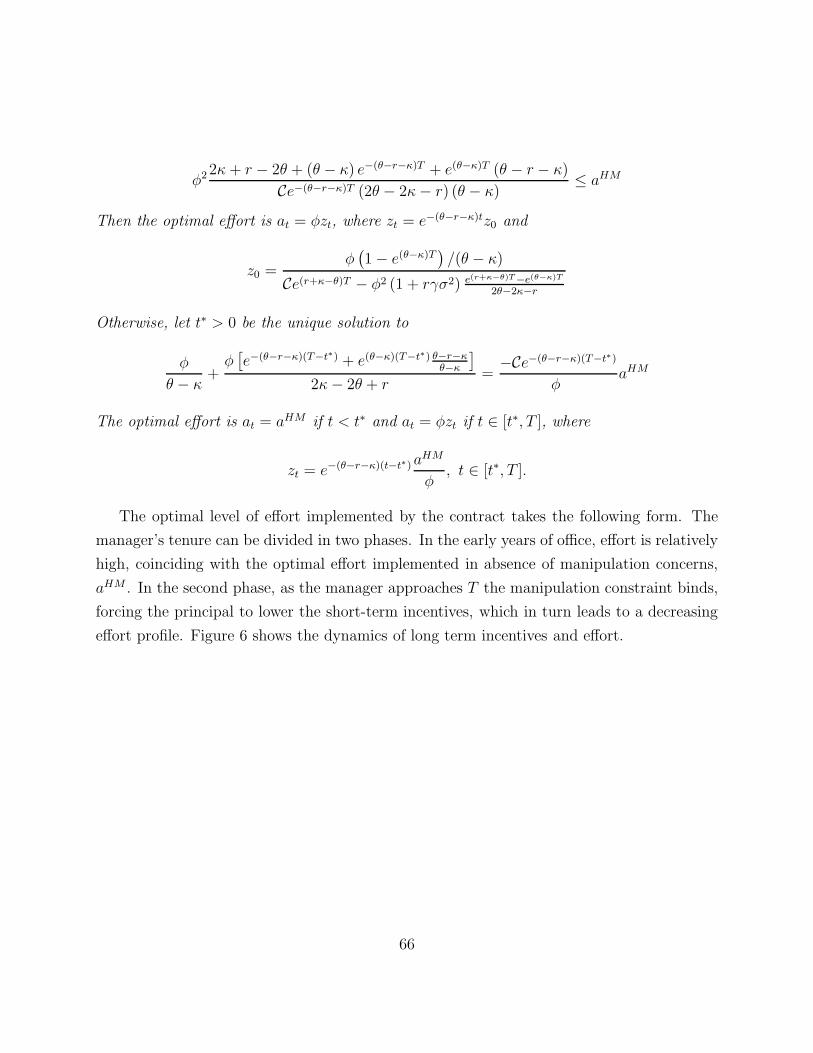
φ22κ+ r − 2θ + (θ − κ) e−(θ−r−κ)T + e(θ−κ)T (θ − r − κ)

Ce−(θ−r−κ)T (2θ − 2κ− r) (θ − κ)≤ aHM

Then the optimal effort is at = φzt, where zt = e−(θ−r−κ)tz0 and

z0 =φ(

1− e(θ−κ)T)

/(θ − κ)

Ce(r+κ−θ)T − φ2 (1 + rγσ2) e(r+κ−θ)T−e(θ−κ)T

2θ−2κ−r

Otherwise, let t∗ > 0 be the unique solution to

φ

θ − κ+φ[

e−(θ−r−κ)(T−t∗) + e(θ−κ)(T−t∗) θ−r−κ

θ−κ

]

2κ− 2θ + r=

−Ce−(θ−r−κ)(T−t∗)

φaHM

The optimal effort is at = aHM if t < t∗ and at = φzt if t ∈ [t∗, T ], where

zt = e−(θ−r−κ)(t−t∗)aHM

φ, t ∈ [t∗, T ].

The optimal level of effort implemented by the contract takes the following form. The

manager’s tenure can be divided in two phases. In the early years of office, effort is relatively

high, coinciding with the optimal effort implemented in absence of manipulation concerns,

aHM . In the second phase, as the manager approaches T the manipulation constraint binds,

forcing the principal to lower the short-term incentives, which in turn leads to a decreasing

effort profile. Figure 6 shows the dynamics of long term incentives and effort.

66

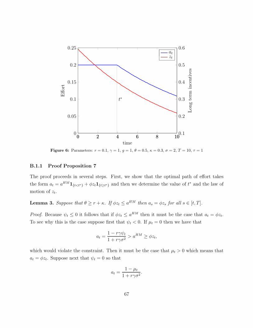
0 2 4 6 8 100

0.05

0.1

0.15

0.2

0.25

0 2 4 6 8 100.1

0.2

0.3

0.4

0.5

0.6

t∗

time

Effort

Lon

gterm

incentives

atatzt

Figure 6: Parameters: r = 0.1, γ = 1, g = 1, θ = 0.5, κ = 0.3, σ = 2, T = 10, τ = 1

B.1.1 Proof Proposition 7

The proof proceeds in several steps. First, we show that the optimal path of effort takes

the form at = aHM1{t<t∗} + φzt1{t≥t∗} and then we determine the value of t∗ and the law of

motion of zt.

Lemma 3. Suppose that θ ≥ r + κ. If φzt ≤ aHM then as = φzs for all s ∈ [t, T ].

Proof. Because ψt ≤ 0 it follows that if φzt ≤ aHM then it must be the case that at = φzt.

To see why this is the case suppose first that ψt < 0. If µt = 0 then we have that

at =1− rγψt1 + rγσ2

> aHM ≥ φzt,

which would violate the constraint. Then it must be the case that µt > 0 which means that

at = φzt. Suppose next that ψt = 0 so that

at =1− µt

1 + rγσ2.

67

If µt = 0, we have at = aHM which can only satisfy the constraint if φzt = aHM , in which

case the equality at = φzt is trivially satisfied. On the other hand, if φzt < aHM then it must

be the case that µt > 0 which implies that at = φzt. Hence, we can conclude that at = φzt.

The next step is to show that as = φzs for s ∈ (s, T ]. Replacing at = φzt in the law

of motion for zt we get that zt = (r + κ − rγφ)zt = (r + κ − θ)zt ≤ 0. Hence, we have

that φzs ≤ aHM for some h and all s ∈ (t, t + h). Repeating the same argument we get

that at+h = φzt+h and zt+h ≤ 0 so we can conclude that φzs ≤ anm and so as = φzs for all

s ∈ [t, T ].

Lemma 4. Let t∗ ≡ inf{t ∈ [0, T ] : φzt ≤ aHM}. The solution to the optimal control problem

is at = aHM if t ∈ [0, t∗) and at = φzt if t ∈ [t∗, T ].

Proof. We have already proven in Lemma 3 that at = φzt for t ∈ [t∗, T ]. Hence, the only

step left is to show that at = aHM for t < t∗. If φz0 ≤ aHM then by Lemma 3 we have t∗ = 0

and there is nothing to prove. Suppose next that φz0 > aHM . Using the initial condition

ψ0 = 0 we get that the optimal effort at time zero satisfies the first order condition

a0 =1− rγψ0 − µ0

1 + rγσ2=

1− µ0

1 + rγσ2≤ aHM .

If µt > 0 then we have φz0 = a0 < aHM which contradicts the hypothesis that φz0 > aHM .

Thus, we can conclude that µ0 = 0 and a0 = aHM . Replacing in the law of motion of ψt we

get that ψ0 = 0 and ψ0 = 0. This means that we can extend the previous argument to the

interval [0, t∗) and get ψt = 0, µt = 0, and at = aHM for all t ∈ [0, t∗).

Proof of Proposition 7 Using the previous two lemmas, we can solve for the optimal

path of effort, for t < t∗ we have that ψt = 0, at = aHM , and

zt = (r + κ)zt − rγaHM .

For t ≥ t∗ we have that at = φzt

zt = (r + κ− θ)zt,

68

and

ψt = −κψt − φµt,

where µt = 1 − rγψt − (1 + rγσ2)φzt. In addition, the system of equations satisfies the

terminal condition ψT = −CzT . For t ≥ t∗, the solution is

zt = e−(θ−r−κ)(t−t∗)zt∗ .

Solving for ψt and using the initial condition ψt∗ = 0 we get

ψ (t) =φ

θ − κ+φ[

e−(−r−κ+θ)(t−t∗) + e(θ−κ)(t−t∗) θ−r−κ

θ−κ

]

−2θ + 2κ + r(38)

Using the terminal condition we get the equation ψT = −CzT t∗ = 0 if and only if

φz0 ≤ aHM which means that t∗ = 0 if and only if

φ2−2θ + 2κ+ r + (θ − κ) e−(−r−κ+θ)T + e(θ−κ)T (θ − r − κ)

−Ce−(θ−r−κ)T (−2θ + 2κ+ r) (θ − κ)≤ aHM

If this condition is not satisfied, then t∗ > 0 and zt∗ = aHM/φ. Using this relation, we get

that t∗ is the unique solution to

φ2

θ − κ+φ2[

e−(−r−κ+θ)(T−t∗) + e(θ−κ)(T−t∗) θ−r−κ

θ−κ

]

−2θ + 2κ+ r= −Ce−(θ−r−κ)(T−t∗)aHM

Given t∗, we can find z0 solving the differential equation

zt = (r + κ)zt − rγaHM ,

with the terminal condition zt∗ = aHM/φ. This yields,

zt =

[

rγ

κ+ r−

(θ − r − κ)e−(r+κ)(t∗−t)

(r + κ)φ

]

aHM

B.2 Optimal Deterministic Contract

In the remainder of this section we analyze the principal’s optimization problem. We solve the

problem using Pontryagin’s maximum principle. Once again, as in Appendix B.1, because

69

the objective function is concave, and the dynamics and mixed constraint are linear, the

necessary conditions in the maximum principle are also sufficient. The principal optimization

problem reduces to

maxz0,at,mt≥0

∫ T

0e−rtπ(at, mt)dt− e−rT 1

2Cz2T

subject to

zt = (r + κ)zt − rγat

mt ≥at−φzt

g,

(39)

where

π(a,m) ≡ a− λm−gm2

2−

(1 + rγσ2) a2

2.

This is an optimal control problem with mixed state constraints. The main challenge posed

by this problem is the determination of the time intervals over which manipulation is positive

and the manipulation constraint binds. We solve for the optimal path in closed form (up to

the solution of a nonlinear equation). The current value Hamiltonian for this optimal control

problem is

H(zt, at, mt, ψt) = π(at, mt) + ψt((r + κ)zt − rγat).

We incorporate the different constraints by considering the augmented Hamiltonian

L(zt, at, mt, ψt, ηt, νt) = H(zt, at, mt, ψt) + ηt

(

mt −at − φzt

g

)

+ νtmt

where ηt and νt are Lagrange multipliers. The co-state variable ψt solves the initial value

problem

ψt = −κψt −φ

gηt, ψ0 = 0.

together with the transversality condition ψT = −CzT . By maximizing the augmented

Hamiltonian, we find that effort and manipulation solves the first order conditions

1−(

1 + rγσ2)

at − rγψt −ηtg

= 0

−λ− gmt + ηt + νt = 0

70

and the complementary slackness conditions

ηt = 0 if mt >at − φzt

g

νt = 0 if mt > 0.

If mt > 0 then νt = 0 so effort is

at =g − λ+ φzt − rγgψt1 + g (1 + rγσ2)

. (40)

This equation shows the determinants of effort. The relation between effort and ψt is in-

tuitive: recall that ψt < 0 represents the shadow marginal cost of providing long-term

incentives. The level of effort is higher when maintaining long term incentives is more costly

because the firm has stronger incentives to accelerate vesting of long-term incentives. Simi-

larly, providing more long term incentives (higher zt) leads to higher effort as we can increase

the amount of effort while keeping manipulation at moderate levels. Manipulation is interior

only if mt = (at − φzt)/g > 0 which requires that at > φzt. Replace at we find the condition

g − λ− rγgψtg (1 + rγσ2)

≥ φzt (41)

If this condition is not satisfied, then mt = 0 and we must consider the two cases that we

already considered in Appendix B.1: i) at = φzt and ii) at > φzt. If the solution is given by

case i), then the multiplier ηt is determined by the first order condition for at and

ηt = g(

1−(

1 + rγσ2)

φzt − rγψt)

. (42)

The optimality condition is satisfied only if the multiplier ηt in (42) is positive. If neither

inequality (41) holds nor ηt > 0, then the solution must be such at < φzt, which means that

ηt = 0 so

at =1− rγψt1 + rγσ2

.

Figure 7 provides a summary of the previous analysis and illustrates the optimal effort and

manipulation for different combinations of (zt, ψt) as we move through the phase diagram.

71

0

at > φzt

mt > 0

at = φzt

mt = 0

at < φzt

mt = 0

−Czt

(z0, ψ0)

(zT , ψT )

zt

ψt

Figure 7: This figure summarizes the optimal effort and manipulation as we move through the phasediagram. There are three regions: in the first region we have positive manipulation, in the second regionwe have zero manipulation and effort is determined by the binding no-manipulation constraint, in thefinal region we have zero manipulation and the no-manipulation constraint is slack.

If we replace the solution for (at, mt) in the differential equation for (zt, ψt), we find a

linear system of ordinary differential equations that can be solved in closed form for each

time interval identified in the proposition. We identify the thresholds t∗ and t∗∗ using the

transversality condition and pasting the solution for (zt, ψt) in the different intervals. The

proof of Proposition 6 follows from an analysis of the behavior of this dynamic system as we

move through the three regions identified in Figure 7. In particular, in Figure 7, we show

that the system moves through the phase diagram from the northeast towards the southwest.

The detailed formal analysis is provided next.

B.2.1 Proof Proposition 6

We start with 3 claims that we will use extensively in the proof.

Claim 1 If φzt > aHM and ψt = 0 then at = aHM , mt = 0 and ψt = 0.

72

Proof. Suppose that mt > 0. If this is the case, then we have that

at − φzt =g − λ+ φzt

1 + g(1 + rγσ2)− φzt

=g − λ− φztg(1 + rγσ2)

1 + g(1 + rγσ2)

<g − λ− aHMg(1 + rγσ2)

1 + g(1 + rγσ2)

=−λ

1 + g(1 + rγσ2)≤ 0,

which implies that mt < 0, contradiction. Accordingly, we have

at =1− rγψt1 + rγσ2

= aHM .

Hence, we have that mt = 0 > at − φzt which yields η = 0. Replacing in the law of motion

for ψt we find that ψt = 0.

Claim 2 If φzt ∈[

1−λ/g−rγψt/g1+rγσ2

, aHM]

then at = φzt, mt = 0 and zt ≤ 0.

Proof. Suppose that mt > 0, then at − φzt < 0 which means that mt < 0 a contradiction.

Hence, it must be the case that mt = 0. Using the first order condition a we get

at =1 + η/g

1 + rγσ2.

If η = 0 we get at = aHM which violates the constraint at ≤ φzt for mt = 0. Hence, it must

be the case that η > 0, which means that at = φzt. Replacing in the ODE for zt we get

zt ≤ 0.

Claim 3 φzt <1−λ/g−rγψt/g

1+rγσ2⇒ mt > 0, and zt < 0.

Proof. Suppose that mt = 0, then we have that η = 0 and

at =1− rγψt1 + rγσ2

≥ aHM > φzt

73

which means that the constraint at ≤ φzt is violated. Thus, we have that mt > 0, ηt > 0

and at > φzt. Using the law of motion of zt we get that

zt = (r + κ)zt − rγat < (r + κ)zt − rγφzt = (r + κ− θ)zt ≤ 0.

Proof Proposition 6 The first step is to show that φz0 ≤ θr+κ

aHM . Suppose this is not

the case, then we have that φz0 >θ

r+κaHM > aHM . By Claim 1 we have that a0 = aHM ,

ψ0 = 0 and z0 > 0. Repeating the same argument at any time t we find that φzt > aHM ,

at = aHM and ψt = 0, all t ∈ [0, T ]. However, this violates the transversality condition

ψT = −Ψ′(zT ).

The previous upper bound implies that we only need to consider three cases:

Case 1: φz0 ∈ [aHM , θr+κ

aHM ]

Case 2: φz0 ∈[

1−λ/g1+rγσ2

, aHM]

Case 3: φz0 <1−λ/g1+rγσ2

First, we consider Case 1. From Claim 1 we have that a0 = aHM , z0 ≤ 0 and ψ0 = 0. We

can also conclude from Claim 1 that at = aHM , zt ≤ 0 and ψt = 0 for all t ∈ [0, t∗] where

t∗ = inf{t > 0 : φzt < aHM}, where it must be the case that t∗ < T because otherwise

ψT = 0 which violates the transversality condition.

Next, Claim 2 implies that that at∗ = φzt∗ , mt∗ = 0 and zt∗ ≤ 0. Let’s define t∗∗ =

inf{t > 0 : φzt <1−λ/g−rγψt/g

1+rγσ2}. If t∗∗ > T then there is nothing else to prove. Hence,

suppose that t∗∗ < T . Claim 2 implies that at = φzt, mt = 0 and zt ≤ 0 for all t ∈ [t∗, t∗∗].

Next, we show that it is also the case that ψt < 0, all t ∈ [t∗, t∗∗]. Using the law of motion

of ψt we get that ψt∗ < 0. Differentiating ψt we get that

ψt = −κψt −φ

gηt,

where

ηt = g − g(

1 + rγσ2)

at − ψtrγg = g − g(

1 + rγσ2)

φzt − ψtrγg

74

so

ηt = −g(

1 + rγσ2)

φzt − ψrγg.

Suppose there is t ∈ [t∗, t∗∗] such that ψt > 0, then there is t < t such that ψt = 0. Replacing

in the law of motion of η and ψt we find that ηt > 0 and ψt < 0. Hence, ψt can never cross

zero which means that ψt < 0 for all t ∈ [t∗, t∗∗].

The final step is to analyze the behavior of (zt, ψt) for t ∈ [t∗∗, T ]. We know that

zt∗∗ < 0 and ψt∗∗ ≤ 0, which means that ddt

(

φzt −1−λ/g−rγψt/g

1+rγσ2}) ∣

∣

∣

t=t∗∗< 0. Accordingly,

φzt <1−λ/g−rγψt/g

1+rγσ2for t ∈ (t∗∗, t∗∗ + ǫ). Claim 3 implies that mt > 0 and zt < 0 for all

t ∈ (t∗∗, t∗∗ + ǫ). Differentiating ψt, we get that

ψt = −κψt −φ

gηt = −κψt − φmt.

Differentiating the solution for mt we get that ψt = 0 implies mt < 0. Thus, ψt = 0 implies

ψt < 0 which implies that ψt < 0 for all t ∈ (t∗∗, t∗∗+ǫ). We can repeat the argument beyond

t∗∗ + ǫ to conclude that mt > 0, zt < 0, ψt < 0 all t ∈ (t∗∗, T ]. Manipulation is given by

mt =g − λ+ φzt − rγgψt1 + g (1 + rγσ2)

− φzt

=g − λ− φg (1 + rγσ2) zt − rγgψt

1 + g (1 + rγσ2)

Hence, we get that

mt = −φg (1 + rγσ2) zt + rγgψt

1 + g (1 + rγσ2)> 0.

Thus, whenever φz0 ∈ [aHM , θr+κ

aHM ] the contract satisfies all the properties in Proposition

6.

We conclude the proof considering Cases 2 and 3. For Case 2, we repeat the argument

in Case 1 using the initial condition ψ0 = 0 and setting t∗ = 0, and for Case 3 we repeat the

argument Case 1 using the initial condition ψ0 = 0 and setting t∗∗ = 0.

75

B.3 Closed Form Solution Optimal Deterministic Contract

The first step is to solve the case with mt > 0, all t ∈ [0, T ]. That is, we start looking at the

solution assuming that the inequality φz0 <1−λ/g1+rγσ2

holds.

Whenever effort and manipulation are interior they solve the first order condition

at =g − λ+ φzt − rγgψt1 + g (1 + rγσ2)

mt =at − φzt

g.

Replacing (at, mt) in the differential equation for zt and ψt we arrive to the forward-backward

differential equations

(

zt

ψt

)

= −

rγ(g−λ)1+g(1+rγσ2)

λφg+ φ(g−λ)

g(

1+g(1+rγσ2))

+

(

r + κ− θ1+g(1+rγσ2)

r2γ2g1+g(1+rγσ2)

φ2 1+rγσ2

1+g(1+rγσ2)θ

1+g(1+rγσ2)− κ

)(

zt

ψt

)

with the initial condition ψ0 = 0 and terminal condition ψT = −CzT . The eigenvalues of the

system are

µ− =1

2

(

r −D

1 + g(1 + rγσ2)

)

µ+ =1

2

(

r +D

1 + g(1 + rγσ2)

)

where

D ≡

√

4θ2g (1 + rγσ2) +(

(r + 2κ)(

1 + g(1 + rγσ2))

− 2θ)2.

with the associated eigenvectors are

v− =

(

(r+2κ)(1+g(1+rγσ2))−2θ−D

2φ2(1+rγσ2)

1

)

and

v+ =

(

(r+2κ)(1+g(1+rγσ2))−2θ+D

2φ2(1+rγσ2)

1

)

76

Hence, by the theory of linear system of differential equations with constant coefficients

we get that he solution is given by

(

zt

ψt

)

=

(

z

ψ

)

+ A−v−eµ−t + A+v+eµ

+t,

where v ≡ (v− v+),

(

z

ψ

)

=

(

r + κ− θ1+g(1+rγσ2)

r2γ2g1+g(1+rγσ2)

φ2

g− φ2

g(1+g(1+rγσ2))θ

1+g(1+rγσ2)− κ

)−1

rγ(g−λ)1+g(1+rγσ2)

λφg+ φ(g−λ)(

1+g(1+rγσ2))

and (A−, A+) constants to be determined. Using the initial conditions ψ0 = 0 and given an

arbitrary initial value z0 we get that

(

A−

A+

)

= v−1

(

z0 − z

−ψ

)

Similarly, using the terminal condition ψT = −CzT we get

(

A−

A+

)

=(

veµT)−1

(

zT − z

−CzT − ψ

)

where veµT ≡ (eµ−Tv−, eµ

+Tv+). Combining these two expressions for (A−, A+)⊤ we get

and equation for (z0, zT ),

v−1

(

z0 − z

−ψ

)

=(

veµT)−1

(

zT − z

−CzT − ψ

)

Finally, using the previous system of equations, we find that the solution (z0, zT ) is

(

z0

zT

)

=(

v−1e1,−( (

veµT)−1

e1 − C(

veµT)−1

e2)

)−1 (

v−1 −(

veµT)−1)

(

z

ψ

)

,

where e1 = (1, 0)⊤ and e2 = (0, 1)⊤ are the unit vectors. Finally, using Proposition 6 we

check if the condition φz0 <1−λ/g1+rγσ2

is satisfied. The next proposition provides a summary of

77

the solution:

Proposition 8. If the optimal contract implements positive manipulation (mt > 0, all t ∈

[0, T ]) then, the optimal effort and manipulation path are

at =g − λ+ φzt − rγgψt1 + g (1 + rγσ2)

mt =at − φzt

g.

The long-term incentives, zt and the co-state variable, ψt are

(

zt

ψt

)

=

(

z

ψ

)

+ A−v−eµ−t + A+v+eµ

+t,

where

µ− =1

2

(

r −D

1 + g(1 + rγσ2)

)

µ+ =1

2

(

r +D

1 + g(1 + rγσ2)

)

D ≡

√

4θ2g (1 + rγσ2) +(

(r + 2κ)(

1 + g(1 + rγσ2))

− 2θx)2

are the eigenvalues of the system (zt, ψt) and

v− =

(

(r+2κ)(1+g(1+rγσ2))−2θ−D

2φ2(1+rγσ2)

1

)

v+ =

(

(r+2κ)(1+g(1+rγσ2))−2θ+D

2φ2(1+rγσ2)

1

)

are the associated eigenvectors. The long term steady state, (z, ψ) is

(

z

ψ

)

=

(

r + κ− θ1+g(1+rγσ2)

r2γ2g1+g(1+rγσ2)

φ2

g− φ2

g(1+g(1+rγσ2))θ

1+g(1+rγσ2)− κ

)−1

rγ(g−λ)1+g(1+rγσ2)

λφg+ φ(g−λ)

g(

1+g(1+rγσ2))

78

The initial value (z0, ψ0) and the constants (A−, A+) are given by

(

A−

A+

)

= v−1

(

z0 − z

−ψ

)

z0 = e⊤1

(

v−1e1,−( (

veµT)−1

e1 − C(

veµT)−1

e2)

)−1 (

v−1 −(

veµT)−1)

(

z

ψ

)

ψ0 = 0

where v ≡ (v−,v+), veµT ≡ (eµ−Tv−, eµ

+Tv+), and e1 = (1, 0)⊤ and e2 = (0, 1)⊤ denote the

unit vectors.

If the solution in the previous case does not satisfies the inequality φz0 <1−λ/g1+rγσ2

, then it

must be the case that the optimal contract entails φz0 ≥1−λ/g1+rγσ2

. The next step is to solve the

principal optimization problem assuming that φz0 ∈[

1−λ/g1+rγσ2

, aHM]

. In this case, we have to

intervals [0, t∗∗] and (t∗∗, T ]. Using the previous solution of the ode for (zt, ψt), we find that

in the interval (t∗∗, T ) we have

at =g − λ+ φzt − rγgψt1 + g (1 + rγσ2)

mt =at − φzt

g.

and(

zt

ψt

)

=

(

z

ψ

)

+ A−v−eµ−(t−t∗∗) + A+v+eµ

+(t−t∗∗), (43)

where(

A−

A+

)

= v−1

(

zt∗∗ − z

ψt∗∗ − ψ

)

. (44)

Repeating computations similar to the ones we did in Proposition 8 we get the system of

equations

v−1

(

zt∗∗ − z

ψt∗∗ − ψ

)

=(

veµ(T−t∗∗))−1

(

zT − z

−CzT − ψ

)

(45)

79

The solution to this system is:

(

zt∗∗

zT

)

=(

v−1e1,−( (

veµ(T−t∗∗))−1

e1 − C(

veµ(T−t∗∗))−1

e2)

)−1

(46)

×

[

(

v−1 −(

veµ(T−t∗∗))−1)

(

z

ψ

)

− v−1e2ψt∗∗

]

,

and in particular,

zt∗∗ = e⊤1

(

v−1e1,−( (

veµ(T−t∗∗))−1

e1 − C(

veµ(T−t∗∗))−1

e2)

)−1

×

[

(

v−1 −(

veµ(T−t∗∗))−1)

(

z

ψ

)

− v−1e2ψt∗∗

]

. (47)

After solving the system of equations in the interval [t∗∗, T ], we move backward and solve

the solution in the interval [0, t∗∗]. In this interval, we have that at = φzt, which means that

zt = (r + κ− θ)zt; hence, we have that zt = z0e−(θ−r−κ)t. In particular, we have that

zt∗∗ = z0e−(θ−r−κ)t∗∗ .

The next step is to solve for ψt. In the interval [0, t∗∗], the constraint mt ≥ (at − φzt)/g is

binding; thus, we have that the multipliers ηt > 0. In particular, we have that

ηtg

= 1− (1 + rγσ2)at − rγψt = 1− (1 + rγσ2)φzt − rγψt. (48)

Accordingly, ψt solves the following ODE

ψt = (θ − κ)ψt − φ+ (1 + rγσ2)φ2zt, ψ0 = 0. (49)

This equations yields the solution

ψt∗∗ =φ

θ − κ

(

1− e(θ−κ)t∗∗)

−(1 + rγσ2)φ2

2θ − 2κ− r

(

e−(θ−r−κ)t∗∗ − e(θ−κ)t∗∗)

z0 (50)

Step 2 in the proof of Proposition 6 implies that t∗∗ is define as t∗∗ = inf{t > 0 : φzt =

80

1−λ/g−rγψt1+rγσ2

}. Accordingly,

φz0 =1− λ

g+ θ

θ−κ

(

e(θ−κ)t∗∗

− 1)

(1 + rγσ2)e−(θ−r−κ)t∗∗ − (1+rγσ2)θ2θ−2κ−r

(e(θ−κ)t∗∗ − e−(θ−r−κ)t∗∗)(51)

Finally, we can solve for t∗∗ using φz0 in combination with (zt∗∗ , ψt∗∗) and Equation (47).

The following Proposition summarizes the previous computations

Proposition 9. Let t∗∗ > 0 be a solution of the equation

zt∗∗ = e⊤1

(

v−1e1,−( (

veµ(T−t∗∗))−1

e1 − C(

veµ(T−t∗∗))−1

e2)

)−1

×

[

(

v−1 −(

veµ(T−t∗∗))−1)

(

z

ψ

)

− v−1e2ψt∗∗

]

,

where

φz0 =1− λ

g+ θ

θ−κ

(

e(θ−κ)t∗∗

− 1)

(1 + rγσ2)e−(θ−r−κ)t∗∗ − (1+rγσ2)θ2θ−2κ−r

(e−(θ−r−κ)t∗∗ − e(θ−κ)t∗∗)

zt∗∗ = z0e−(θ−r−κ)t∗∗

ψt∗∗ = −φ

θ − κ

(

e(θx−κ)t∗∗

− 1)

−(1 + rγσ2)φ2

2θ − 2κ− r

(

e−(θ−r−κ)t∗∗ − e(θ−κ)t∗∗)

z0.

If φz0 ∈[

1−λ/g1+rγσ2

, aHM]

and t∗∗ ≤ T , then the solution to the Principal’s problem is at = φzt,

mt = 0, zt = z0e−(θ−r−κ)t, all t ∈ [0, t∗∗], and

at =g − λ+ φzt − rγgψt1 + g (1 + rγσ2)

mt =at − φzt

g

for t ∈ (t∗∗, T ], where

(

zt

ψt

)

=

(

z

ψ

)

+ A−v−eµ−(t−t∗∗) + A+v+eµ

+(t−t∗∗),

81

and(

A−

A+

)

= v−1

(

zt∗∗ − z

ψt∗∗ − ψ

)

.

If t∗∗ > T and

φz0 =φ2

θ−κ

(

e(θx−κ)T − 1)

Ce−(θ−r−κ)T − (1+rγσ2)φ2

2θ−2κ−r(e−(θ−r−κ)T − e(θ−κ)T )

∈

[

1− λ/g

1 + rγσ2, aHM

]

then, at = φzt and mt = 0 for all t ∈ [0, T ].

The final case is when φz0 > aHM . In this case, we have that at = aHM up to time

t∗ = inf{t > 0 : φzt = aHM}. The value of zt at time t ∈ [0, t∗] is given by

zt = z0e(r+κ)t −

rγaHM

r + κ

(

e(r+κ)t − 1)

.

Hence, we have that

φzt∗ = φz0e(r+κ)t∗ −

θaHM

r + κ

(

e(r+κ)t∗

− 1)

= aHM .

Replacing z0 by zt∗ in Proposition 9 and using the condition aHM = φzt∗ we get that the

solution to the Principal problem is

Proposition 10. Let 0 < t∗ < t∗∗ be a solution to

aHM =1− λ

g+ θ

θ−κ

(

e(θ−κ)(t∗∗−t∗) − 1

)

(1 + rγσ2)e−(θ−r−κ)(t∗∗−t∗) − (1+rγσ2)θ2θ−2κ−r

(e−(θ−r−κ)(t∗∗−t∗) − e(θx−κ)(t∗∗−t∗))

zt∗∗ = e⊤1

(

v−1e1,−( (

veµ(T−t∗∗))−1

e1 − C(

veµ(T−t∗∗))−1

e2)

)−1

×

[

(

v−1 −(

veµ(T−t∗∗))−1)

(

z

ψ

)

− v−1e2ψt∗∗

]

,

82

where

zt∗∗ =aHM

φe−(θ−r−κ)(t∗∗−t∗)

ψt∗∗ = −φ

θ − κ

(

e(θx−κ)(t∗∗−t∗) − 1

)

−(1 + rγσ2)φ

2θ − 2κ− r

(

e−(θ−r−κ)(t∗∗−t∗) − e(θ−κ)(t∗∗−t∗)

)

aHM .

The initial condition z0 is given by

φz0 = aHM[

e−(r+κ)t∗ +θ

r + κ

(

1− e−(r+κ)t∗)

]

.

If φz0 > aHM and t∗∗ ≤ T , then the solution to the Principal’s problem is at = aHM , mt = 0,

all t ∈ [0, t∗]; at = φzt, mt = 0, zt =aHM

φe−(θ−r−κ)(t−t∗), all t ∈ [t∗, t∗∗], and

at =g − λ+ φzt − rγgψt1 + g (1 + rγσ2)

mt =at − φzt

g

for t ∈ (t∗∗, T ], where

(

zt

ψt

)

=

(

z

ψ

)

+ A−v−eµ−(t−t∗∗) + A+v+eµ

+(t−t∗∗),

and(

A−

A+

)

= v−1

(

zt∗∗ − z

ψt∗∗ − ψ

)

.

If t∗∗ > T and there is t∗ such that

aHM =φ2

θ−κ

(

e(θx−κ)(T−t∗) − 1

)

Ce−(θ−r−κ)(T−t∗) − (1+rγσ2)φ2

2θ−2κ−r(e−(θ−r−κ)(T−t∗) − e(θ−κ)(T−t∗))

then mt = 0, all t ∈ [0, T ], at = aHM , all t ∈ [0, t∗], at = φzt, all t ∈ (t∗, T ] and

φz0 = aHM(

e−(r+κ)t +θ

r + κ

(

1− e−(r+κ)t)

)

83

C Numerical Computation HJB Equation

In this section we describe the numerical approach based on Barles and Souganidis (1991)

(See Forsyth and Vetzal (2012) and Tourin (2013) for a more applied exposition with a focus

on financial applications). We start writing the HJB equation in a way more suitable for

computation. For computational purposes, it is convenient to measure the time backward,

so we let s = T − t, and define the value function f(z, s) = F (z, T − s). The infinitesimal

generator is

La,σzf = [(r + κ)z + arγ(σσz − 1)]fz +1

2σzfzz − rf,

so the HJB equation can be writen as

fs = maxa∈[0,a]σz

{

La,σzf + π(a, z)}

with a Dirichlet boundary condition

f(z, 0) = −1

2Cz2

The upper bound β implies that zt is bounded so we can restrict the domain of the value

function to a finite region. Unless τ = ∞, the upper bound on zt varies over time. For

the numerical implementation, it is convenient to consider a constant upper bound. On the

other hand, the free disposal assumption implies that βt ≥ 0 so zt ≥ 0 (Formally, the free

disposal implies that βt ≥ 0 for t ≤ T . In principle, it could be possible that βt < 0 for

t > T so zt < 0 for some t ≤ T . However, it is easy to verify that it is never optimal to let

zt to become negative on [0, T ]). Thus, we consider z ∈ Q ≡ [0, Zmax] for some large Zmax.

Notice that, if we let TQ ≡ inf{t > 0 : zt /∈ Q}, we have that T ∧ TQ → T when Zmax → ∞,

which means that we can choose Zmax large enough so the constraint has an arbitrarily small

effect on the solution of the contract. This type of boundary condition is suggested as an

alternative by Kushner and Dupuis (2013). This means that we solve the problem

F (z, 0) = supa,σz

E

[∫ T∧TQ

0

e−rtπ(at, zt)dt− e−rT1

2Cz2T1T≤TQ + e−rTQF (zTQ, TQ)1T>TQ

]

84

subject to

dzt = [(r + κ)zt + rγat(σσzt − 1)]dt+ σztdBt

mt ≥at − φzt

g

mt ≥ 0,

where {0, Zmax} are absorbing boundaries. Accordingly, at {0, Zmax} the condition dzt = 0

must be satisfied so σz = 0 and amax = (r + κ)Zmax/rγ when z = Zmax and a = 0 when

z = 0. Thus, the value function at the boundaries is given by

f(0, s) = 0

f(Zmax, s) =π(

amax,max{

0, amax−φZmax

g

})

r

(

1− e−rs)

− e−rs1

2CZ2

max.

We solve the partial differential equation using finite differences. We introduce the uni-

form grid {z0, . . . , zNz} such that z0 = Zmin and zNz = Zmax and zi+1 − zi = h for all

0 ≤ i ≤ Nz − 1. Similarly, we consider the grid for the time variable {s0, . . . , sNs} such that

s0 = 0, sNs = T and sn+1 − sn = ∆s for all 0 ≤ n ≤ Ns − 1. We denote the value function

at the grid point (zi, sn) by fni .

Next, we discretize the infinitesimal generator using an upwind scheme: In particular,

we use the discretization

(La,σzh fn+1)i = α(a, σz, zi)fn+1i+1 + ρ(a, σz, zi)

σz2h2

fn+1i−1 − (α(a, σz, zi) + ρ(a, σz , zi) + r) fn+1

i .

where

α(a, σz, zi) =

σz2h2

+ (r+κ)zi+arγ(σσz−1)h

if σz2h2

+ (r+κ)zi+arγ(σσz−1)h

> 0

σz2h2

otherwise

ρ(a, σz , zi) =

σz2h2

if σz2h2

+ (r+κ)zi+arγ(σσz−1)h

> 0

σz2h2

− (r+κ)zi+arγ(σσz−1)h

otherwise

The previous discretization is such that whenever σz2h2

+ (r+κ)zi+arγ(σσz−1)h

> 0 we have

85

(La,σzh fn+1)i = [(r + κ)zi + arγ(σσz − 1)]fn+1i+1 − fn+1

i

h+

1

2σzfn+1i+1 − 2fn+1

i + fn+1i−1

h2− rfn+1

i .

and whenever σz2h2

+ (r+κ)zi+arγ(σσz−1)h

≤ 0 we have

(La,σzh fn+1)i = [(r + κ)zi + arγ(σσz − 1)]fn+1i − fn+1

i−1

h+

1

2σzfn+1i+1 − 2fn+1

i + fn+1i−1

h2− rfn+1

i .

That is, the discretization La,σzh switches between forward and backward difference approx-

imation of the derivatives to guarantee that the coefficients α(a, σz, zi) and ρ(a, σz, zi) are

always positive. The finite difference version of the HJB equation is

fn+1i − fni

∆s= max

a, σz

{

(La,σzh fn+1)i + π (a, zi)}

, (52)

The previous discretization is stable, consistent, and monotone, which means that the

discretization (52) converges to the unique viscosity solution (Barles and Souganidis, 1991).

The combination of forward and backward approximations in the discretized operator La,σzh

makes difficult to solve the maximization problem in (52) analytically. We discretize the

control set and consider controls in the grids a ∈ {0, . . . , aK} and σz ∈ {σz0, . . . , σzK}. Notice

that once we have approximated the value function, we can use the closed form solution for

the maximization in the original HJB equation to get a more precise approximation of the

policy function. In the numerical implementation we use a uniform grid for a and a non-

uniform grid for σz ; in particular, in the case of σz we use a grid that is finer near σz = 0.

The use of an implicit scheme in (52) requires to solve a highly nonlinear equation at each

time step: We solve this nonlinear equation using policy iteration. Let fn = (fn0 , · · · , fnNz)

be the value unction at the time step n. For n = 0 we set

f 0i = −

1

2Cz2i ,

and for each time step n ≥ 1, we use the following policy iteration algorithm

1. Set (fn+1)0 = fn

2. Set fk = (fn+1)k

86

3. For each i ∈ {1, · · · , Ns − 1}, set

(aki , σkzi) = argmax

a,σz

{

(La,σzh fk)i + π (a, zi)}

4. Find (fn+1)k+1 solving the linear system of equations

(

1−∆sLaki ,σ

kzi

h

)

(fn+1i )k+1 = fni +∆sπ

(

aki , zi)

, i = 1, . . . , Nz − 1

(fn+10 )k+1 = 0

(fn+1Nz

)k+1 = f(Zmax, sn+1),

5. Stop if

maxi

|(fn+1i )k+1 − fki |

max(

1, |(fn+1i )k+1|

) < tolerance,

otherwise go back to step 2.

The previous policy iteration algorithm converges monotonically to the unique solution of

the nonlinear equation.

87