Embed Size (px)
Citation preview
JSS Journal of Statistical SoftwareFebruary 2017, Volume 76, Issue 8. doi: 10.18637/jss.v076.i08
CEoptim: Cross-Entropy R Package forOptimization
Tim BenhamThe University of
Queensland, Brisbane
Qibin DuanThe University of
Queensland, Brisbane
Dirk P. KroeseThe University of
Queensland, Brisbane
Benoît LiquetThe University of
Queensland, Brisbane
Abstract
The cross-entropy (CE) method is a simple and versatile technique for optimization,based on Kullback-Leibler (or cross-entropy) minimization. The method can be applied toa wide range of optimization tasks, including continuous, discrete, mixed and constrainedoptimization problems. The new package CEoptim provides the R implementation of theCE method for optimization. We describe the general CE methodology for optimizationand well as some useful modifications. The usage and efficacy of CEoptim is demonstratedthrough a variety of optimization examples, including model fitting, combinatorial opti-mization, and maximum likelihood estimation.
Keywords: constrained optimization, continuous optimization, cross-entropy, discrete opti-mization, Kullback-Leibler divergence, lasso, maximum likelihood, R, regression.
1. IntroductionThe cross-entropy (CE) method originates from an adaptive variance minimization algorithmin Rubinstein (1997) for the estimation of rare event probabilities in stochastic networks. Itwas realized in Rubinstein (1999) that many optimization problems could be converted intorare-event estimation problems, providing a rare-event based approach to optimization, wherea sequence of probability densities is generated that converges to a degenerate density thatconcentrates its mass close to the optimizer.Generally, the CE method involves two iterative phases:
1. Generation of a set of random samples (vectors, trajectories, etc.) according to a spec-ified parameterized model.
2. Updating of the model parameters, based on the best samples generated in the previousstep. This is done by Kullback-Leibler (also called cross-entropy) minimization.
2 CEoptim: Cross-Entropy R Package for Optimization
Since the appearance of the CE monograph (Rubinstein and Kroese 2004) and tutorial(De Boer, Kroese, Mannor, and Rubinstein 2005), the CE method has continued to de-velop and has been successfully applied to a great variety of difficult optimization problems,including motion planning in robotic systems (Kobilarov 2012), electricity network gener-ation, (Kothari and Kroese 2009), control of infectious diseases (Sani and Kroese 2008),buffer allocation (Alon, Kroese, Raviv, and Rubinstein 2005), Laguerre tessellation (Duan,Kroese, Brereton, Spettl, and Schmidt 2014), and network reliability (Kroese, Hui, and Nar-iai 2007). An extensive list of recent work can be found in Botev, Kroese, Rubinstein, andL’Ecuyer (2013). Websites that provide MATLAB (The MathWorks Inc. 2014) code includehttp://www.cemethod.org/ and http://www.montecarlohandbook.org/. Since R (R CoreTeam 2016) has become an essential tool for statistical computation, it is useful to provide anaccessible implementation of the CE method for R users, similar to R packages for simulatedannealing (Xiang, Gubian, Suomela, and Hoeng 2013), evolutionary methods (Mullen, Ardia,Gil, Windover, and Cline 2011), and particle swarm optimization methods (Bendtsen 2012).Some advantages of the CE method are:
• The CE method is a global optimization method which is particularly useful when theobjective function has many local optima.
• The CE method can be used to solve continuous, discrete, and mixed optimizationproblems, which may also include constraints.
• The CE code is extremely compact and is readily written in native R, making furtherdevelopment and modifications easy to implement.
• The CE method is based on rigorous mathematical and statistical principles.
Our aim is not to replace the standard optimization solvers such as optim and nlm but toprovide a viable alternative in cases where standard gradient or simplex-based solvers arenot applicable (e.g., when the optimization problem contains both discrete and continuousvariables) or are expected to do poorly (e.g., when there are many local optima).The rest of this paper is organized as follows. In Section 2, we sketch the general theory behindthe CE method, which leads to the basic CE algorithm. In Section 3, we describe a varietyof optimization scenarios, including continuous, discrete and constrained mixed problems, towhich CE can be applied effectively. The description and usage of the CEoptim package(Benham, Duan, Kroese, and Liquet 2017) are given in Section 4. Section 5 demonstratesthe capability of the package through a range of numerical examples. In the final section wemake concluding remarks for CEoptim.
2. CE method for optimizationLet X be an arbitrary set of states and let S be a real-valued performance function on X .Suppose the goal is to find the minimum of S over X , and the corresponding minimizer x∗(assuming, for simplicity, that there is only one). Denote the minimum by γ∗, so that
S(x∗) = γ∗ = minx∈X
S(x). (1)
Journal of Statistical Software 3
The CE methodology for optimization is adapted from the CE methodology for rare eventestimation in the following way. Associate with the above problem (1) the estimation ofthe probability ` = P(S(X) ≤ γ), where X has some probability density f(x; u) on X (forexample corresponding to the uniform distribution on X ) depending on a parameter u anda level γ. Thus, for optimization problems randomness is deliberately introduced in orderto make the model stochastic. If γ is chosen close to the unknown γ∗, then ` is typicallya rare-event probability. One of the most effective ways to estimate rare-event probabilitiesis to use importance sampling. In particular, to estimate ` = P(S(X) ≤ γ) one can use theimportance sampling estimator
ˆ= 1N
N∑i=1
f(Xi)g(Xi)
I{S(Xi) ≤ γ},
where X1, . . . ,XN are iid samples from a well-chosen importance sampling density g. Theoptimal importance sampling density is in this case g∗(x) = f(x)I{S(x) ≤ γ}/`, which givesa zero-variance estimator, but depends on the unknown quantity `. The main idea behind theCE method for estimation is to adaptively determine an importance sampling pdf f(x; v∗) –hence within the same family as the original distribution – that is close to g∗ in Kullback-Leibler sense. Specifically, a parameter v∗ is sought that minimizes the cross-entropy distance
D(g∗, f(·; v)) = Eg∗
[log g∗(X)
f(X; v)
]=∫g∗(x) log g∗(x) dx−
∫g∗(x) log f(x; v) dx .
This is equivalent to maximizing, with respect to v,∫f(x; u)I{S(x) ≤ γ} log f(x; v) dx = Eu [I{S(X) ≤ γ} log f(X; v)] ,
which in turn can be estimated by maximizing the sample average
1N
N∑i=1
[I{S(Xi) ≤ γ} log f(Xi; v)] , (2)
where X1, . . . ,XN is an iid sample from f(x; u). This is, in essence, maximum likelihoodestimation. In particular, (2) gives the maximum likelihood estimator of v based on onlythe samples X1, . . . ,XN that have a function value less than or equal to γ. These are theso-called elite samples.The relevance to optimization is that when γ is close to the (usually unknown) minimumγ∗, then the importance sampling density g∗ concentrates most of its mass in the vicinity ofthe minimizer x∗. Sampling from such a distribution thus produces optimal or near-optimalstates. The CE method for optimization produces a sequence of levels (γt) and referenceparameters (vt) determined from (2) such that the former tends to the optimal γ∗ and thelatter to the optimal reference vector v∗, where f(x; v∗) corresponds to the point mass at x∗;see, e.g., Rubinstein and Kroese (2017, page 251).The generic steps for CE optimization are specified in Algorithm 1.
To run the algorithm, one needs to provide the class of sampling densities {f(·; v)}, the initialvector v0, the sample size N , the rarity parameter ρ, and the stopping criterion. It is prudentto keep track of the overall best function value and corresponding state, and report these at
4 CEoptim: Cross-Entropy R Package for Optimization
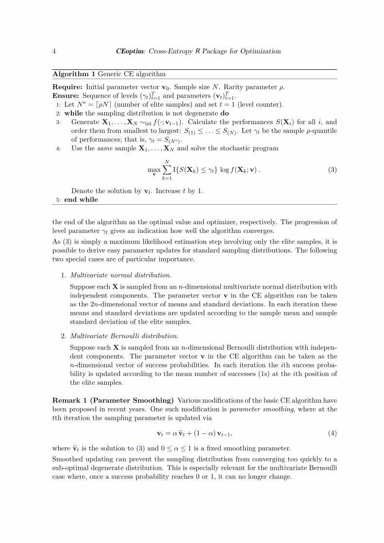
Algorithm 1 Generic CE algorithm
Require: Initial parameter vector v0. Sample size N . Rarity parameter ρ.Ensure: Sequence of levels (γt)Tt=1 and parameters (vt)Tt=1.
1: Let N e = dρNe (number of elite samples) and set t = 1 (level counter).2: while the sampling distribution is not degenerate do3: Generate X1, . . . ,XN ∼iid f(·; vt−1). Calculate the performances S(Xi) for all i, and
order them from smallest to largest: S(1) ≤ . . . ≤ S(N). Let γt be the sample ρ-quantileof performances; that is, γt = S(Ne).
4: Use the same sample X1, . . . ,XN and solve the stochastic program
maxv
N∑k=1
I{S(Xk) ≤ γt} log f(Xk; v) . (3)
Denote the solution by vt. Increase t by 1.5: end while
the end of the algorithm as the optimal value and optimizer, respectively. The progression oflevel parameter γt gives an indication how well the algorithm converges.As (3) is simply a maximum likelihood estimation step involving only the elite samples, it ispossible to derive easy parameter updates for standard sampling distributions. The followingtwo special cases are of particular importance.
1. Multivariate normal distribution.Suppose each X is sampled from an n-dimensional multivariate normal distribution withindependent components. The parameter vector v in the CE algorithm can be takenas the 2n-dimensional vector of means and standard deviations. In each iteration thesemeans and standard deviations are updated according to the sample mean and samplestandard deviation of the elite samples.
2. Multivariate Bernoulli distribution.Suppose each X is sampled from an n-dimensional Bernoulli distribution with indepen-dent components. The parameter vector v in the CE algorithm can be taken as then-dimensional vector of success probabilities. In each iteration the ith success proba-bility is updated according to the mean number of successes (1s) at the ith position ofthe elite samples.
Remark 1 (Parameter Smoothing) Various modifications of the basic CE algorithm havebeen proposed in recent years. One such modification is parameter smoothing, where at thetth iteration the sampling parameter is updated via
vt = α vt + (1− α) vt−1, (4)
where vt is the solution to (3) and 0 ≤ α ≤ 1 is a fixed smoothing parameter.Smoothed updating can prevent the sampling distribution from converging too quickly to asub-optimal degenerate distribution. This is especially relevant for the multivariate Bernoullicase where, once a success probability reaches 0 or 1, it can no longer change.
Journal of Statistical Software 5
It is also possible to use different smoothing parameters for different components of theparameter vector (e.g., the means and the standard deviations). Note that the smoothingparameters for means and standard deviations should not be very small. When setting thesmoothing parameters too small, the means would be improved very slowly and it would takemuch longer to run before the standard deviation converged.
Remark 2 (Choice of sampling densities) Although sampling distributions with inde-pendent components are the most convenient to use in a CE implementation, it is sometimesadvantageous to consider more complex sampling models, such as mixture models. In thiscase the updating of parameters (maximum likelihood estimation) may no longer be triv-ial, but one can instead employ fast methods such as the EM algorithm to determine theparameter updates.
Remark 3 (Choice of the CE parameters) The CE method is fairly robust with respectto the choice of the parameters. The rarity parameter ρ is typically chosen between 0.01 and0.1. The number of elite samples N e = dρNe should be large enough to obtain a reliableparameter update in (3). For example, if the dimension of v is d, the number of elites shouldbe in the order of 10 d or higher.
3. Optimization scenariosIn this section we consider a number of optimization scenarios to which CEoptim could beapplied.
3.1. Continuous optimization
Consider a continuous optimization problem with state space X = Rn. The sampling distri-bution on Rn can be quite arbitrary and does not need to be related to the objective functionS. Usually, the random vector X = (X1, . . . , Xn)> ∈ Rn is generated from a Gaussian distri-bution with independent components, characterized by a vector µ of means and a vector σof standard deviations. At each iteration of the CE method, these vectors of parameters areupdated as the means and standard deviations of the elite samples. During the course of thealgorithm a sequence of (µt) and (σt) are generated, such that µt tends to the optimizer x∗,while the vector of standard deviations tends to the zero vector. At the end of the algorithmone should obtain a degenerate probability density with mean µT approximately equal to theoptimizer x∗ and all standard deviations close to 0. A possible stopping criterion is to stopwhen all components in σT are smaller than some ε. This scheme is referred to as normalupdating.CEoptim implements the normal updating scheme for continuous optimization.
3.2. Discrete optimization
If the state space X is finite, the optimization problem is often referred to as a discrete orcombinatorial optimization problem, where X could be the space of combinatorial objects,such as binary vectors, trees, graphs, etc. To apply the CE method to a discrete optimizationproblem, one needs a conveniently parameterized random mechanism to generate samples.
6 CEoptim: Cross-Entropy R Package for Optimization
For discrete optimization CEoptim implements sampling from state spaces X of the form{0, 1, . . . , c1 − 1} × · · · × {0, 1, . . . , cn − 1}, where the {ci} are strictly positive integers. Thecomponents of the random vector X = (X1, . . . , Xn)> ∈ X are taken to be independent, sothat its distribution is determined by a sequence of probability vectors p1, . . . ,pn, with thejth component of pi corresponding to pij = P(Xi = j). For a given elite sample set E of sizeN e, the CE updating formulas for these probabilities are
pij =∑
X∈E I{Xi = j}N e , i = 1, . . . , n, j = 0, . . . , cn − 1, (5)
where I denotes the indicator function. Hence at each iteration probability pij is updatedsimply as the average number of times that the ith component of the elite vectors is equalto j. A possible stopping rule for a discrete optimization problem is to stop when the overallbest objective value does not change over a number of iterations. Alternatively, one couldstop when the sampling distribution has degenerated sufficiently; for example, when all {pij}are no further than ε away from either 0 or 1.
3.3. Constrained optimization
The general optimization problem (1) also covers constrained optimization, where the searchspace X could, for example, be defined by a system of inequalities:
Gi(x) ≤ 0, i = 1, . . . , k. (6)
One way to deal with constraints is to use acceptance-rejection: Generate a random vectorX on a simple search space that contains X , and accept or reject it based on whether thesample falls into X or not. Alternatively, one could try to sample directly from a truncateddistribution on X , e.g., using Gibbs sampling.CEoptim implements linear constraints for continuous optimization of the form Ax ≤ b,where A is a matrix and b a vector. The program will use either acceptance-rejection or Gibbssampling to sample from the multivariate normal distribution truncated to the constraint set.A second approach to handle constraints is to introduce a penalty function. For example, forthe constraints (6), the objective function could be modified to
S(x) = S(x) +k∑i=1
Hi max{Gi(x), 0}, (7)
where Hi < 0 measures the importance of the ith penalty. To use the penalty approach withCEoptim the user simply needs to modify the objective function according to (7). The choiceof the penalty constants {Hi} is problem specific and may need to be determined by trial anderror.
4. CEoptim descriptionIn this section we describe how to use CEoptim. The CEoptim function is the main function ofthe package CEoptim. It can be used to solve continuous and discrete optimization problemsas well as mixtures thereof.

Journal of Statistical Software 7
4.1. Usage
CEoptim(f, f.arg = NULL, maximize = FALSE, continuous = NULL,discrete = NULL, N = 100L, rho = 0.1, iterThr = 1e4L, noImproveThr = 5,verbose = FALSE)
4.2. Arguments
f : Function to be optimized. Can have continuous and discrete arguments.
f.arg : List of additional fixed arguments passed to function f.
maximize : Logical value determining whether to maximize or minimize the objective func-tion.
continuous : List of arguments for the continuous optimization part, consisting of:
• mean: Vector of initial means.• sd: Vector of initial standard deviations.• smoothMean: Smoothing parameter for the vector of means. Default value 1 (no
smoothing).• smoothSd: Smoothing parameter for the standard deviations. Default value 1 (no
smoothing).• sdThr: Positive numeric convergence threshold. Check whether the maximum
standard deviation is smaller than sdThr. Default value 0.001.• conMat: Coefficient matrix of linear constraint conMat x ≤ conVec.• conVec: Value vector of linear constraint conMat x ≤ conVec.
discrete : List of arguments for the discrete optimization part, consisting of:
• categories: Integer vector which defines the allowed values of the categorical vari-ables. The ith categorical variable takes values in the set {0, 1, . . . , categories(i)−1}.
• probs: List of initial probabilities for the categorical variables. Defaults to equal(uniform) probabilities.
• smoothProb: Smoothing parameter for the probabilities of the categorical samplingdistribution. Default value 1 (no smoothing).
• probThr: Positive numeric convergence threshold. Check whether all probabilitiesin the categorical sampling distributions deviate less than probThr from either 0or 1. Default value 0.001.
N : Integer representing the CE sample size.
rho : Value between 0 and 1 representing the elite proportion.
iterThr : Termination threshold on the largest number of iterations.

8 CEoptim: Cross-Entropy R Package for Optimization
noImproveThr : Termination threshold on the largest number of iterations during which noimprovement of the best function value is found.
verbose : Logical value set for CE progress output.
4.3. Value
CEoptim returns a list with the following components.
optimum : Optimal value of f.
optimizer : The location of the optimal value. A list consisting of:
• continuous: Continuous part of the optimizer.• discrete: Discrete part of the optimizer.
termination : Termination information. A list consisting of:
• niter: Total number of iterations upon termination.• nfe: Total number of function evaluations.• convergence: One of the following termination statements:
– Not converged, if the number of iterations reaches iterThr.– The optimum did not change for noImproveThr iterations, if the best
value has not improved for noImproveThr iterations.– Variances converged, otherwise.
states : List of intermediate results computed at each iteration. It consists of the iterationnumber (iter), the best overall value (optimum) and the worst value of the elite samples,(gammat). The means (mean) and maximum standard deviation (maxSd) of the elite setare also included for continuous cases, and the maximum deviations (maxProbs) of thesampling probabilities to either 0 or 1 are included for discrete cases.
states.probs : List of categorical sampling probabilities computed at each iteration. Willonly be returned for discrete and mixed cases.
4.4. Note
• Although partial parameter passing is allowed outside lists, it is recommended thatparameter names be specified in full. Parameters inside lists have to be specified com-pletely.
• Because CEoptim is function internally using pseudo-random number generation it isuseful to (1) set the seed for the random number generator (for testing purposes), and(2) investigate the quality of the results by repeating the optimization a number oftimes.
Journal of Statistical Software 9
5. Numerical examplesThe following examples illustrate the use, flexibility, and efficacy of the CEoptim functionfrom the package CEoptim.
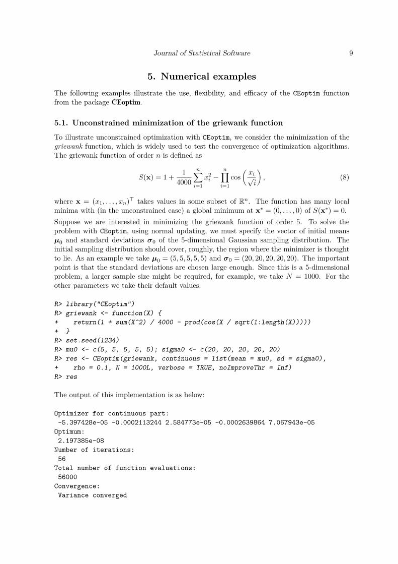
5.1. Unconstrained minimization of the griewank function
To illustrate unconstrained optimization with CEoptim, we consider the minimization of thegriewank function, which is widely used to test the convergence of optimization algorithms.The griewank function of order n is defined as
S(x) = 1 + 14000
n∑i=1
x2i −
n∏i=1
cos(xi√i
), (8)
where x = (x1, . . . , xn)> takes values in some subset of Rn. The function has many localminima with (in the unconstrained case) a global minimum at x∗ = (0, . . . , 0) of S(x∗) = 0.Suppose we are interested in minimizing the griewank function of order 5. To solve theproblem with CEoptim, using normal updating, we must specify the vector of initial meansµ0 and standard deviations σ0 of the 5-dimensional Gaussian sampling distribution. Theinitial sampling distribution should cover, roughly, the region where the minimizer is thoughtto lie. As an example we take µ0 = (5, 5, 5, 5, 5) and σ0 = (20, 20, 20, 20, 20). The importantpoint is that the standard deviations are chosen large enough. Since this is a 5-dimensionalproblem, a larger sample size might be required, for example, we take N = 1000. For theother parameters we take their default values.
R> library("CEoptim")R> griewank <- function(X) {+ return(1 + sum(X^2) / 4000 - prod(cos(X / sqrt(1:length(X)))))+ }R> set.seed(1234)R> mu0 <- c(5, 5, 5, 5, 5); sigma0 <- c(20, 20, 20, 20, 20)R> res <- CEoptim(griewank, continuous = list(mean = mu0, sd = sigma0),+ rho = 0.1, N = 1000L, verbose = TRUE, noImproveThr = Inf)R> res
The output of this implementation is as below:
Optimizer for continuous part:-5.397428e-05 -0.0002113244 2.584773e-05 -0.0002639864 7.067943e-05
Optimum:2.197385e-08
Number of iterations:56
Total number of function evaluations:56000
Convergence:Variance converged

10 CEoptim: Cross-Entropy R Package for Optimization
Remark 4 (Extraction and print method) The user could easily extract any output us-ing:
R> res$optimum
[1] 2.197385e-08
R> res$optimizer$continuous
[1] -5.397428e-05 -0.0002113244 2.584773e-05 -0.0002639864 7.067943e-05
The print method for ‘CEoptim’ objects provides by default the main description of the‘CEoptim’ object including: optimizer; optimum; termination. To get the states andstates.probs outputs, one should set the corresponding arguments to TRUE. The user couldalso specify the output to print:
R> print(res, optimum = TRUE)
Optimum:2.197385e-08
5.2. Constrained minimization of the griewank function
To illustrate constrained optimization with CEoptim, we wish to minimize the griewank func-tion of order 2 over the triangle with vertex points (1, 4), (4, 0), and (8, 4); see Figure 1.The constraint set can be written as the linearly constrained region {x ∈ R2 : Ax ≤ b} with
A =
0 1−1 −1
1 1
and b =
4−4
4
.To solve the problem with CEoptim we proceed as follows:
R> library("CEoptim")R> set.seed(123)R> griewank <- function(X) {+ return(1 + sum(X^2) / 4000 - prod(cos(X / sqrt(1:length(X)))))+ }R> A <- rbind(c(0,1), c(-1,-1), c(1,-1))R> b <- c(4, -4, 4)R> res <- CEoptim(griewank, continuous = list(mean = c(0,0), sd = c(10,10),+ conMat = A, conVec = b), rho = 0.1, N = 200L, verbose = TRUE,+ noImproveThr = Inf)R> cat("direct optimizer = ", res$optimizer$continuous, "\n")R> cat("direct minimum = ", res$optimum, "\n")

Journal of Statistical Software 11
−2 0 2 4 6 8 10
−1
01
23
45
Figure 1: Contour plot of the griewank function and the triangular constraint region. Theoptimal solution (indicated by a cross) lies on the boundary of the constraint region.
The corresponding output shows that the minimum is obtained at the boundary of the trian-gle.
direct minimizer = 3.139669 3.991955direct minimum = 0.05685487
It is also possible to use a penalty approach for this problem. Here we take the penaltyfunction
S(x) = S(x) + 100 ‖Ax− b‖,
which can be implemented in the following way.
R> griewank.penalty <- function(X, A, b) {+ fn <- griewank(X)+ if (any(A %*% as.vector(X) > b)) {+ penalty <- norm(A %*% as.vector(X) - b)+ fn <- fn + 100 * penalty+ }+ return(fn)+ }
The optimization now proceeds as follows (note that we have also changed rho and N):
R> set.seed(123)R> res.pen <- CEoptim(griewank.penalty, f.arg = list(A, b),+ continuous = list(mean = c(0, 0), sd = c(10, 10)), rho = 0.01,+ N = 2000L, verbose = TRUE, noImproveThr = Inf)
12 CEoptim: Cross-Entropy R Package for Optimization
0 5 10 15 20
−3
−2
−1
01
23
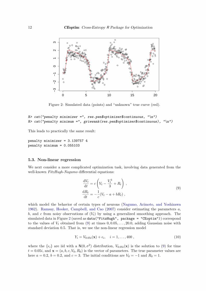
Figure 2: Simulated data (points) and “unknown” true curve (red).
R> cat("penalty minimizer =", res.pen$optimizer$continuous, "\n")R> cat("penalty minimum =", griewank(res.pen$optimizer$continuous), "\n")
This leads to practically the same result:
penalty minimizer = 3.139757 4penalty minimum = 0.055103
5.3. Non-linear regression
We next consider a more complicated optimization task, involving data generated from thewell-known FitzHugh-Nagumo differential equations:
dVtdt = c
(Vt −
V 3t
3 +Rt
),
dRtdt = −1
c(Vt − a+ bRt) ,
(9)
which model the behavior of certain types of neurons (Nagumo, Arimoto, and Yoshizawa1962). Ramsay, Hooker, Campbell, and Cao (2007) consider estimating the parameters a,b, and c from noisy observations of (Vt) by using a generalized smoothing approach. Thesimulated data in Figure 2 (saved as data("FitzHugh", package = "CEoptim")) correspondto the values of Vt obtained from (9) at times 0, 0.05, . . . , 20.0, adding Gaussian noise withstandard deviation 0.5. That is, we use the non-linear regression model
Yi = V0.05i(x) + εi, i = 1, . . . , 400 , (10)
where the {εi} are iid with a N(0, σ2) distribution, V0.05i(x) is the solution to (9) for timet = 0.05i, and x = (a, b, c, V0, R0) is the vector of parameters. The true parameter values arehere a = 0.2, b = 0.2, and c = 3. The initial conditions are V0 = −1 and R0 = 1.

Journal of Statistical Software 13
Estimation of the parameters via the CE method can be established by minimizing the least-squares performance
S(x) =400∑i=0
(yi − V0.05i(x))2 , (11)
where the {yi} are the simulated data from the model (10). Note that we assume also thatthe initial conditions are unknown.We use the deSolve package (Soetaert, Petzoldt, and Setzer 2010) to numerically solve theFitzHugh-Nagumo differential equations (9). Hereto, we first define the function FN.
R> FN <- function(t, state, parameters) {+ with(as.list(c(state, parameters)), {+ dV <- c * (V - V^3/3 + R)+ dR <- -1 / c * (V - a + b * R)+ list(c(dV, dR))+ })+ }
The following function ssres now implements the objective function in (11).
R> ssres <- function(x, fundf, times, y) {+ parameters <- c(a = x[1], b = x[2], c = x[3])+ state <- c(V = x[4], R = x[5])+ out <- ode(y = state, times = times, func = fundf, parms = parameters)+ return(sum((out[, 2] - y)^2))+ }
CEoptim could be used with µ0 = (0, 0, 5, 0, 0) and σ0 = (1, 1, 1, 1, 1). Constant smoothingparameters α = 0.9 and β = 0.5 were used for the {µt} and the {σt} respectively. To see theprogress of the algorithm we set verbose to TRUE. The other arguments remain default.
R> library("deSolve")R> library("CEoptim")R> set.seed(123405)R> times <- seq(0, 20, by = 0.05)R> data("FitzHugh", package = "CEoptim")R> res <- CEoptim(ssres, f.par = list(fundf = FN, times = times, y = ySim),+ continuous = list(mean = c(0, 0, 5, 0, 0), sd = c(1, 1, 1, 1, 1),+ smoothMean = 0.9, smoothSd = 0.5), verbose = TRUE)
The final output is as follows:
R> res
Optimizer for continuous part:0.1959748 0.2395983 3.001453 -0.9938222 0.9791585
Optimum:102.8005
14 CEoptim: Cross-Entropy R Package for Optimization
−0.4−0.2 0.0 0.2 0.4 0.6 0.8 010
020
030
040
0
15 20 25 30 35 40 45
First parameter
Itera
tionDen
sity
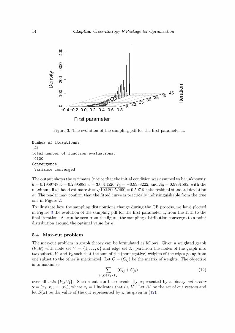
Figure 3: The evolution of the sampling pdf for the first parameter a.
Number of iterations:41
Total number of function evaluations:4100
Convergence:Variance converged
The output shows the estimates (notice that the initial condition was assumed to be unknown):a = 0.1959748, b = 0.2395983, c = 3.0014526, V0 = −0.9938222, and R0 = 0.9791585, with themaximum likelihood estimate σ =
√102.8005/400 = 0.507 for the residual standard deviation
σ. The reader may confirm that the fitted curve is practically indistinguishable from the trueone in Figure 2.To illustrate how the sampling distributions change during the CE process, we have plottedin Figure 3 the evolution of the sampling pdf for the first parameter a, from the 15th to thefinal iteration. As can be seen from the figure, the sampling distribution converges to a pointdistribution around the optimal value for a.
5.4. Max-cut problemThe max-cut problem in graph theory can be formulated as follows. Given a weighted graph(V,E) with node set V = {1, . . . , n} and edge set E, partition the nodes of the graph intotwo subsets V1 and V2 such that the sum of the (nonnegative) weights of the edges going fromone subset to the other is maximized. Let C = (Cij) be the matrix of weights. The objectiveis to maximize ∑
(i,j)∈V1×V2
(Cij + Cji) (12)
over all cuts {V1, V2}. Such a cut can be conveniently represented by a binary cut vectorx = (x1, x2, . . . , xn), where xi = 1 indicates that i ∈ V1. Let X be the set of cut vectors andlet S(x) be the value of the cut represented by x, as given in (12).
Journal of Statistical Software 15
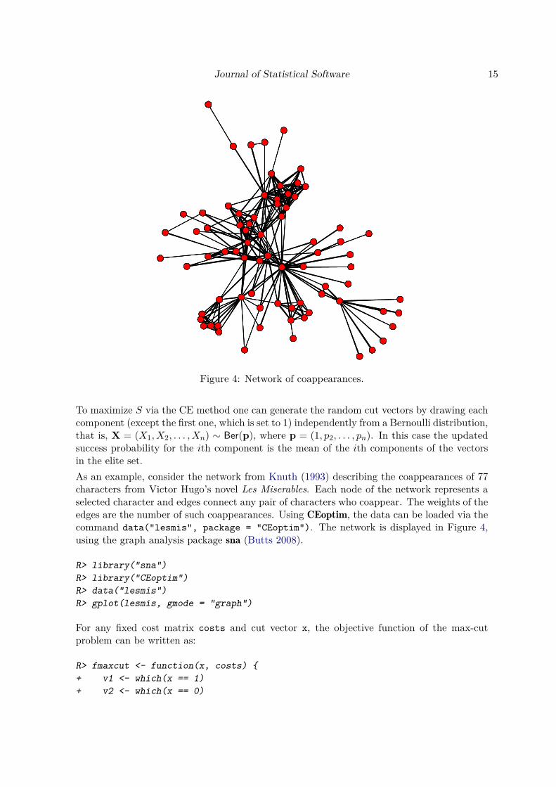
Figure 4: Network of coappearances.
To maximize S via the CE method one can generate the random cut vectors by drawing eachcomponent (except the first one, which is set to 1) independently from a Bernoulli distribution,that is, X = (X1, X2, . . . , Xn) ∼ Ber(p), where p = (1, p2, . . . , pn). In this case the updatedsuccess probability for the ith component is the mean of the ith components of the vectorsin the elite set.As an example, consider the network from Knuth (1993) describing the coappearances of 77characters from Victor Hugo’s novel Les Miserables. Each node of the network represents aselected character and edges connect any pair of characters who coappear. The weights of theedges are the number of such coappearances. Using CEoptim, the data can be loaded via thecommand data("lesmis", package = "CEoptim"). The network is displayed in Figure 4,using the graph analysis package sna (Butts 2008).
R> library("sna")R> library("CEoptim")R> data("lesmis")R> gplot(lesmis, gmode = "graph")
For any fixed cost matrix costs and cut vector x, the objective function of the max-cutproblem can be written as:
R> fmaxcut <- function(x, costs) {+ v1 <- which(x == 1)+ v2 <- which(x == 0)
16 CEoptim: Cross-Entropy R Package for Optimization
+ return(sum(costs[v1, v2]))+ }
To optimize this function with the CEoptim package, we specify the following arguments:discrete$probs = {(0,1); (0.5.0.5);...;(0.5,0.5)}, sample size N = 3000 and opti-mization type: maximize = TRUE. To see the output we set verbose = TRUE. The otherarguments are taken as default. Note that users only need to specify either categories orprobs; if both of them are specified, then categories will be overridden.
R> set.seed(5)R> p0 <- list()R> for (i in 1:77) {+ p0 <- c(p0, list(rep(0.5, 2)))+ }R> p0[[1]] <- c(0, 1)R> res <- CEoptim(fmaxcut, f.arg = list(costs = lesmis), maximize = TRUE,+ verbose = TRUE, discrete = list(probs = p0), N = 3000L)R> ind <- res$optimizer$discreteR> group1 <- colnames(lesmis)[which(ind == TRUE)]R> group2 <- colnames(lesmis)[which(ind == FALSE)]
The output of CEoptim is as follows:
R> res
Optimizer for discrete part:1 0 1 0 0 0 0 0 0 0 1 0 0 1 1 1 0 0 1 1 0 1 01 0 1 1 1 1 0 0 1 1 1 1 1 1 0 0 0 0 1 0 1 0 01 0 1 1 1 0 1 1 1 0 0 0 0 1 1 0 1 0 0 1 1 1 10 0 1 0 1 0 0 0
Optimum:535
Number of iterations:20
Total number of function evaluations:60000
Convergence:Optimum did not change for 5 iterations
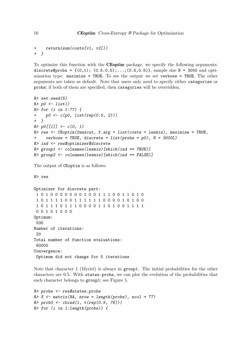
Note that character 1 (Myriel) is always in group1. The initial probabilities for the othercharacters are 0.5. With states.probs, we can plot the evolution of the probabilities thateach character belongs to group1; see Figure 5.
R> probs <- res$states.probsR> X <- matrix(NA, nrow = length(probs), ncol = 77)R> prob0 <- cbind(1, t(rep(0.5, 76)))R> for (i in 1:length(probs)) {
Journal of Statistical Software 17
t=0
Index
0.5
t=1
Index
0.5
t=2
Index
0.5
t=3
Index
0.5
t=4
0.5
t=5
Index
0.5
t=9
Index
0.5
t=13
Index0.
5
t=17
Index
0.5
t=21
0.5
Figure 5: Evolution of categorical sampling probabilities that characters in group 1.
+ for (j in 1:77) {+ X[i, j] <- res$states.probs[[i]][[j]][2]+ }+ }R> X <- rbind(prob0, X)R> par(mfcol = c(5, 2), mar = c(1, 1.5, 1, 1.5), oma = c(1, 1, 1, 1))R> for (i in 1:5) {+ plot(X[i, ], type = "h", lwd = 4, col = "blue", ylim = c(0, 1),+ xaxt = "n", yaxt = "n", ylab = "",+ main = paste("t=", i - 1, sep = ""))+ axis(2, at = 0.5, labels = 0.5)+ }R> for (i in 1:5) {+ plot(X[1 + 4 * i, ], type = "h", lwd = 4, col = "blue",+ ylim = c(0, 1), xaxt = "n", yaxt = "n", ylab = "",+ main = paste("t=", 1 + 4 * i, sep = ""))+ axis(2, at = 0.5, labels = 0.5)+ }
Based on the output above, the two groups of characters are indicated in Table 1: We ranthe program 1000 times with different inital random number generator seeds. In 312 casesthe optimal solution (535) was found. The frequency of the results of CEoptim is given inFigure 6.
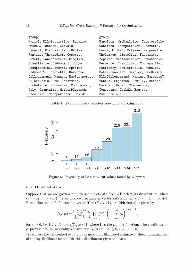
18 CEoptim: Cross-Entropy R Package for Optimization
group1 group2Myriel, MlleBaptistine, Labarre,MmeDeR, Isabeau, Gervais,Fameuil, Blacheville , Dahlia,Fantine, Thenardier, Cosette,Javert, Fauchelevent, Simplice,Scaufflaire, Oldwoman1, Judge,Champmathieu, Brevet, Eponine,Oldwoman2, Jondrette, Gavroche,Gillenormand, Magnon, MmePontmercy,MlleVaubois, LtGillenormand,Combeferre, Prouvaire, Courfeyrac,Joly, Grantaire, MotherPlutarch,Gueulemer, Montparnasse, Child1
Napoleon, MmeMagloire, CountessDeLo,Geborand, Champtercier, Cravatte,Count, OldMan, Valjean, Marguerite,Tholomyes, Listolier, Favourite,Zephine, MmeThenardier, Bamatabois,Perpetue, Chenildieu, Cochepaille,Pontmercy, Boulatruelle, Anzelma,MotherInnocent, Gribier, MmeBurgon,MlleGillenormand, Marius, BaronessT,Mabeuf, Enjolras, Feuilly, Bahorel,Bossuet, Babet, Claquesous,Toussaint, Child2, Brujon,MmeHucheloup
Table 1: Two groups of characters providing a maximal cut.
Fre
quen
cy
050
150
250
6 1329
75
128
216 221
312
528 529 530 531 532 533 534 535
Figure 6: Frequency of best max-cut values found by CEoptim.
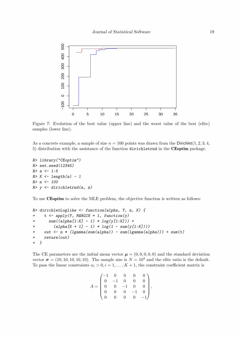
5.5. Dirichlet data
Suppose that we are given a random sample of data from a Dirichlet(α) distribution, whereα = (α1, . . . , αK+1)> is an unknown parameter vector satisfying αi > 0, i = 1, . . . ,K + 1.Recall that the pdf of a random vector Y = (Y1, . . . , YK) ∼ Dirichlet(α) is given by
f(y;α) = Γ(∑K+1i=1 αi)∏K+1
i=1 Γ(αi)
K∏i=1
yαi−1i
(1−
K∑i=1
yi
)αK+1−1
,
for yi ≥ 0, i = 1, . . . ,K and∑Ki=1 yi ≤ 1, where Γ is the gamma function. The conditions on
α provide natural inequality constraints: Gi(α) ≡ −αi ≤ 0, i = 1, . . . ,K + 1.We will use the CE method to obtain the maximum likelihood estimate by direct maximizationof the log-likelihood for the Dirichlet distribution given the data.
Journal of Statistical Software 19
0 5 10 15 20 25 30 35
−10
00
100
200
300
400
500
res$
stat
es[,
"gam
mat
"]
Figure 7: Evolution of the best value (upper line) and the worst value of the best (elite)samples (lower line).
As a concrete example, a sample of size n = 100 points was drawn from the Dirichlet(1, 2, 3, 4,5) distribution with the assistance of the function dirichletrnd in the CEoptim package.
R> library("CEoptim")R> set.seed(12345)R> a <- 1:5R> K <- length(a) - 1R> n <- 100R> y <- dirichletrnd(a, n)
To use CEoptim to solve the MLE problem, the objective function is written as follows:
R> dirichletLoglike <- function(alpha, Y, n, K) {+ t <- apply(Y, MARGIN = 1, function(y)+ sum((alpha[1:K] - 1) * log(y[1:K])) ++ (alpha[K + 1] - 1) * log(1 - sum(y[1:K])))+ out <- n * (lgamma(sum(alpha)) - sum(lgamma(alpha))) + sum(t)+ return(out)+ }
The CE parameters are the initial mean vector µ = (0, 0, 0, 0, 0) and the standard deviationvector σ = (10, 10, 10, 10, 10). The sample size is N = 104 and the elite ratio is the default.To pass the linear constraints αi > 0, i = 1, . . . ,K + 1, the constraint coefficient matrix is
A =
−1 0 0 0 00 −1 0 0 00 0 −1 0 00 0 0 −1 00 0 0 0 −1
,

20 CEoptim: Cross-Entropy R Package for Optimization
and the constraint vector is b = (0, 0, 0, 0, 0). No smoothing parameter is applied to themean vector, but a constant smoothing parameter of smoothSd = 0.5 is applied to each ofthe standard deviations. This is a maximization problem, so we set maximize = TRUE.
R> mu0 <- rep(0, times = K + 1)R> sigma0 <- rep(10, times = K + 1)R> A <- matrix(rep(0, times = 25), nrow = 5)R> diag(A) <- rep(-1, times = 5)R> b <- rep(0, times = 5)R> res <- CEoptim(dirichletLoglike, f.arg = list(Y = y, n = 100, K = 4),+ maximize = TRUE, continuous = list(mean = mu0, sd = sigma0,+ conMat = A, conVec = b, smoothSd = 0.5), N = 10000L, verbose = TRUE)
With the returned states variable, we can plot the evolution of optimal values per iteration,as shown in Figure 7, where the upper line indicates the best value found so far, while thelower line gives the worst value of the current elite sample.
R> par(mai = c(0.6, 1, 0.5, 0.2), oma = c(0, 0, 0, 1))R> plot(res$states[, "iter"], res$states[, "gammat"], type = "s",+ col = "blue", xlab = "", ylab = "")R> lines(res$states[, "optimum"], type = "s", col = "red")R> res
Optimizer for continuous part:1.111656 2.000186 3.534268 3.983616 5.142336
Optimum:486.2124
Number of iterations:35
Total number of function evaluations:350000
Convergence:Variance converged
Maximum likelihood estimates for Dirichlet data can be computed to a high accuracy via thefixed-point techniques of Minka (2012). This requires sophisticated numerical techniques forinverting digamma functions. When applying this method to the same Dirichlet(1, 2, 3, 4, 5)data, we obtained the estimate α = (1.111715, 2.000243, 3.534321, 3.983752, 5.142596), witha likelihood value of 486.2124, giving excellent agreement between the two approaches.
5.6. Lasso regression
Suppose that we observed some data from the following model:
Yi = x>i β + εi, i = 1, . . . , n ,
where xi = (xi1, . . . , xip)> is the p-vector of explanatory variables, β = (β1, . . . , βp)> is the p-vector of regression coefficients, and the {εi} are the noise terms with E[εi] = 0, Var[εi] = σ2,
Journal of Statistical Software 21
for all i and Cov(εi, εj) = 0 (∀i 6= j). Consider a lasso regression approach to estimate theregression vector β:
βlasso = argmin
β∈Rp
12n
n∑i=1
(Yi − x>i β)2 + λp∑j=1|βj |
= argminβ∈Rp
12n‖Y −Xβ‖
22︸ ︷︷ ︸
Loss
+λ ‖β‖1︸ ︷︷ ︸Penalty
,
where Y = (Y1, . . . , Yn)> and X = (x1, . . . ,xn)> is the (n × p) design matrix. The tuningparameter λ controls the amount of regularization.For a given value of λ, we will use the CE method to obtain the lasso regression coefficientand compare our results with those obtained by the function glmnet from the package glmnetpresented by Friedman, Hastie, and Tibshirani (2008).We generate a set of test data of size n = 150, with p = 60 explanatory variables independentlygenerated from a standard normal distribution. The true coefficients β are chosen such that10 are large (between 0.5 and 1) and 50 are exactly 0. The variance of the noise is equal to 1.
R> set.seed(10)R> n <- 150R> p <- 60R> beta <- c(runif(10, 0.5, 1), rep(0, 50))R> X <- matrix(rnorm(n * p), ncol = 60)R> Y <- X %*% matrix(beta, ncol = 1) + rnorm(n)
We first use the glmnet function to find the lasso regression coefficient that gives a sparsityof 10; that is, exactly 10 coefficients are non-zero.
R> library("glmnet")R> res.glmnet <- glmnet(X, Y)R> sparsity.10 <- which(res.glmnet$df == 10)R> (lambda.10 <- res.glmnet$lambda[sparsity.10[1]])
0.2731371
R> beta.glmnet <- res.glmnet$beta[, sparsity.10[1]]
The corresponding indices are correctly identified by glmnet:
R> (ind.beta <- which(res.glmnet$beta[, sparsity.10[1]] != 0))
V1 V2 V3 V4 V5 V6 V7 V8 V9 V101 2 3 4 5 6 7 8 9 10
The values of the non-zero coefficients (NZ) are given by:
R> (beta.glmnet.NZ <- res.glmnet$beta[ind.beta, sparsity.10[1]])

22 CEoptim: Cross-Entropy R Package for Optimization
V1 V2 V3 V4 V5 V60.39006188 0.39345242 0.40795534 0.57510345 0.18776598 0.19553092
V7 V8 V9 V100.02929225 0.55435619 0.57656731 0.56279719
We now use CEoptim to estimate the lasso regression function for the given λ = 0.2731371.
R> library("CEoptim")R> RSS.penalized <- function(x, X, Y, lambda) {+ out <- (1/2) * mean((Y-X %*% matrix(x, ncol = 1, nrow = dim(X)[2],+ byrow = TRUE))**2) + lambda * sum(abs(x))+ return(out)+ }R> mu0 <- rep(0, times = p)R> sigma0 <- rep(5, times = p)R> N <- 1000R> set.seed(1212)R> res <- CEoptim(RSS.penalized, f.arg = list(X = X, Y = Y,+ lambda = lambda.10), continuous = list(mean = mu0, sd = sigma0,+ sdThr = 0.00001), N = N)R> beta.CEoptim <- res$optimizer$continuousR> (ind.beta.CEoptim.NZ <- which(abs(beta.CEoptim) > 0.000001))
[1] 1 2 3 4 5 6 7 8 9 10
R> beta.CEoptinm.NZ <- beta.CEoptim[ind.beta.CEoptim.NZ]R> (compare.beta.NZ <- rbind(beta.glmnet.NZ, beta.CEoptinm.NZ))
V1 V2 V3 V4 V5 V6beta.glmnet.NE 0.3900619 0.3934524 0.4079553 0.5751035 0.1877660 0.1955309beta.CEoptinm.NE 0.3631798 0.3826273 0.4419025 0.6014707 0.1639559 0.1721753
V7 V8 V9 V10beta.glmnet.NE 0.029292247 0.5543562 0.5765673 0.5627972beta.CEoptinm.NE 0.005821685 0.5537388 0.5854710 0.6034473
The two methods give similar values for the non-zero coefficients, although they are notexactly the same. Note, however, that of the two solutions the one found by CEoptim givesthe smaller value for the objective function RSS
2n + λ‖β‖1 (where residual sum of squares:RSS = ‖Y −Xβ‖22).
R> (RSS.penalized(beta.CEoptim, X = X, Y = Y, lambda = lambda.10))
[1] 1.990268
R> (RSS.penalized(beta.glmnet, X = X, Y = Y, lambda = lambda.10))
[1] 1.993622
Journal of Statistical Software 23
0.0 0.2 0.4 0.6 0.8 1.0
0.00
00.
005
0.01
00.
015
λ
RS
S(g
lmne
t)−
RS
S(C
Eop
tim)
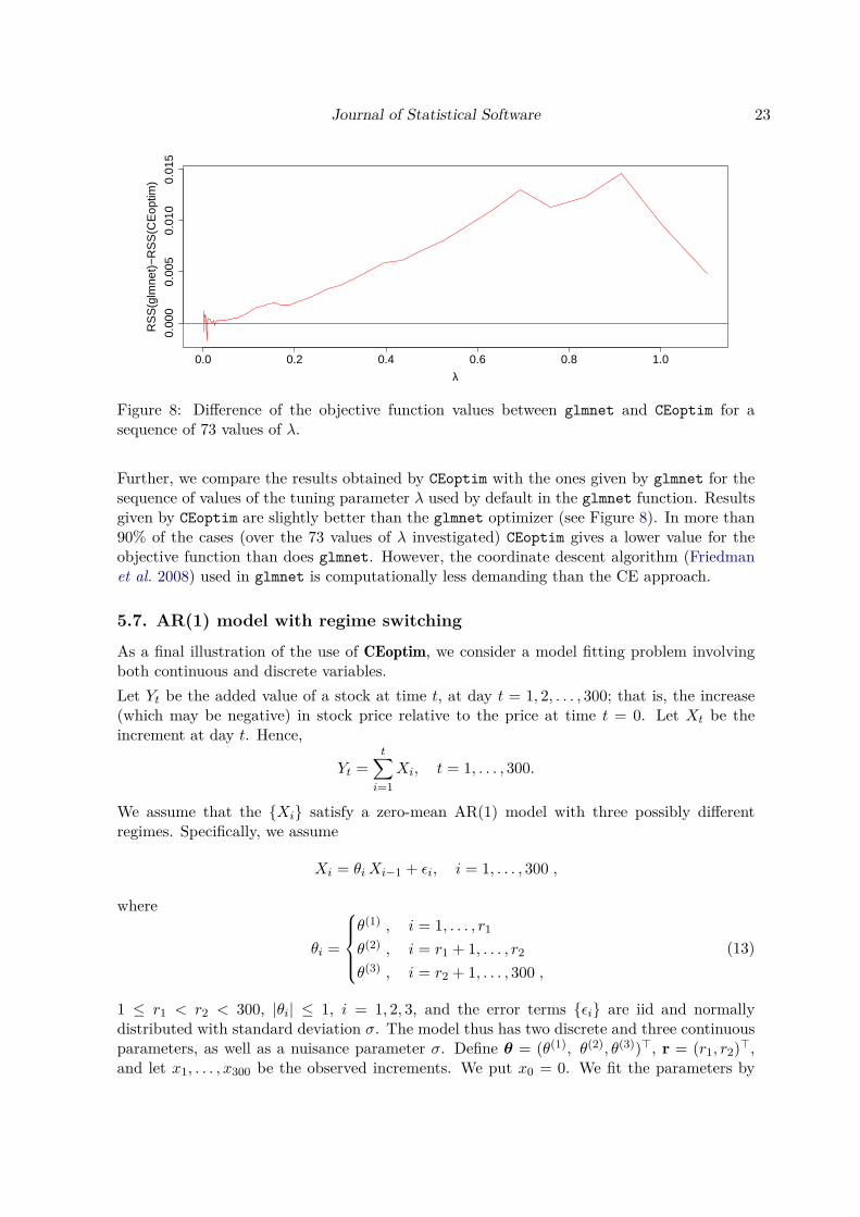
Figure 8: Difference of the objective function values between glmnet and CEoptim for asequence of 73 values of λ.
Further, we compare the results obtained by CEoptim with the ones given by glmnet for thesequence of values of the tuning parameter λ used by default in the glmnet function. Resultsgiven by CEoptim are slightly better than the glmnet optimizer (see Figure 8). In more than90% of the cases (over the 73 values of λ investigated) CEoptim gives a lower value for theobjective function than does glmnet. However, the coordinate descent algorithm (Friedmanet al. 2008) used in glmnet is computationally less demanding than the CE approach.
5.7. AR(1) model with regime switching
As a final illustration of the use of CEoptim, we consider a model fitting problem involvingboth continuous and discrete variables.Let Yt be the added value of a stock at time t, at day t = 1, 2, . . . , 300; that is, the increase(which may be negative) in stock price relative to the price at time t = 0. Let Xt be theincrement at day t. Hence,
Yt =t∑i=1
Xi, t = 1, . . . , 300.
We assume that the {Xi} satisfy a zero-mean AR(1) model with three possibly differentregimes. Specifically, we assume
Xi = θiXi−1 + εi, i = 1, . . . , 300 ,
where
θi =
θ(1) , i = 1, . . . , r1
θ(2) , i = r1 + 1, . . . , r2
θ(3) , i = r2 + 1, . . . , 300 ,(13)
1 ≤ r1 < r2 < 300, |θi| ≤ 1, i = 1, 2, 3, and the error terms {εi} are iid and normallydistributed with standard deviation σ. The model thus has two discrete and three continuousparameters, as well as a nuisance parameter σ. Define θ = (θ(1), θ(2), θ(3))>, r = (r1, r2)>,and let x1, . . . , x300 be the observed increments. We put x0 = 0. We fit the parameters by

24 CEoptim: Cross-Entropy R Package for Optimization
minimizing the least squares function
L(θ, r) =300∑i=1
(xi − xi)2 ,
where xi is the fitted value θi xi−1, and θi is determined by θ and r via (13). The vectorof fitted values, say x, can be written in matrix notation as x = Xθ, where X is a 300 × 3matrix where the elements in rows 1, . . . , r1 in the first column are equal to x0, . . . , xr1−1; theelements in rows r1 + 1, . . . , r2 in the second column are equal to xr1 , . . . , xr2−1; the elementsin rows r2 + 1, . . . , 300 in the third column are equal to xr2 , . . . , x299; and all other elementsare 0. The implementation of the least squares function is given below. Note that the functionrequires input r − 1 rather than r, because each categorical variable used in CEoptim takesvalue in a set {0, . . . , c} for some c.
R> sumsqrs <- function(theta, rm1, x) {+ N <- length(x)+ r <- 1 + sort(rm1)+ if (r[1] == r[2]) {+ return(Inf)+ }+ thetas <- rep(theta, times = c(r, N) - c(1, r + 1) + 1)+ xhat <- c(0, head(x, -1)) * thetas+ sum((x - xhat)^2)+ }
The data were generated using the parameters θ = (0.3, 0.9,−0.9), r = (100, 200) and σ = 0.1.The data are included in the package and are available by using:
R> data("yt", package = "CEoptim")R> xt <- yt - c(0, yt[-300])
The following code implements the use of CEoptim for this constrained mixed problem.
R> A <- rbind(diag(3), -diag(3))R> b <- rep(1, 6)R> set.seed(123)R> library("CEoptim")R> res <- CEoptim(f = sumsqrs, f.arg = list(xt), continuous =+ list(mean = c(0, 0, 0), sd = rep(1.0, 3), conMat = A, conVec = b),+ discrete = list(categories = c(298L, 298L), smoothProb = 0.5),+ N = 10000, rho = 0.001, verbose = TRUE)
The output is as follows:
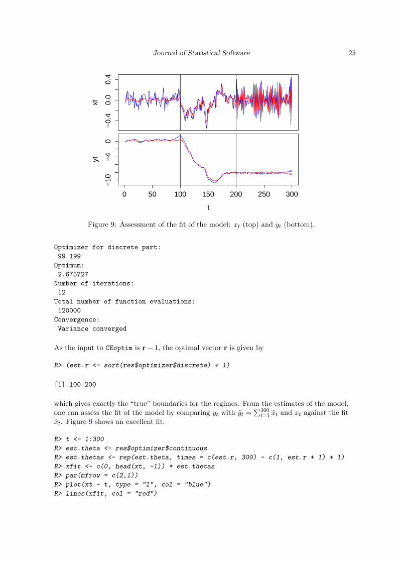
R> res
Optimizer for continuous part:0.2702714 0.8801672 -0.8975874
Journal of Statistical Software 25
−0.
40.
00.
4
xt
0 50 100 150 200 250 300
−10
−4
0
t
yt
Figure 9: Assessment of the fit of the model: xt (top) and yt (bottom).
Optimizer for discrete part:99 199
Optimum:2.675727
Number of iterations:12
Total number of function evaluations:120000
Convergence:Variance converged
As the input to CEoptim is r− 1, the optimal vector r is given by
R> (est.r <- sort(res$optimizer$discrete) + 1)
[1] 100 200
which gives exactly the “true” boundaries for the regimes. From the estimates of the model,one can assess the fit of the model by comparing yt with yt =
∑300i=1 xt and xt against the fit
xt. Figure 9 shows an excellent fit.
R> t <- 1:300R> est.theta <- res$optimizer$continuousR> est.thetas <- rep(est.theta, times = c(est.r, 300) - c(1, est.r + 1) + 1)R> xfit <- c(0, head(xt, -1)) * est.thetasR> par(mfrow = c(2,1))R> plot(xt ~ t, type = "l", col = "blue")R> lines(xfit, col = "red")
26 CEoptim: Cross-Entropy R Package for Optimization
0 50 150 250
−0.
3−
0.1
0.1
Residuals
t
−3 −2 −1 0 1 2 3
−0.
3−
0.1
0.1
Normal Q−Q Plot
Theoretical Quantiles
resi
dual
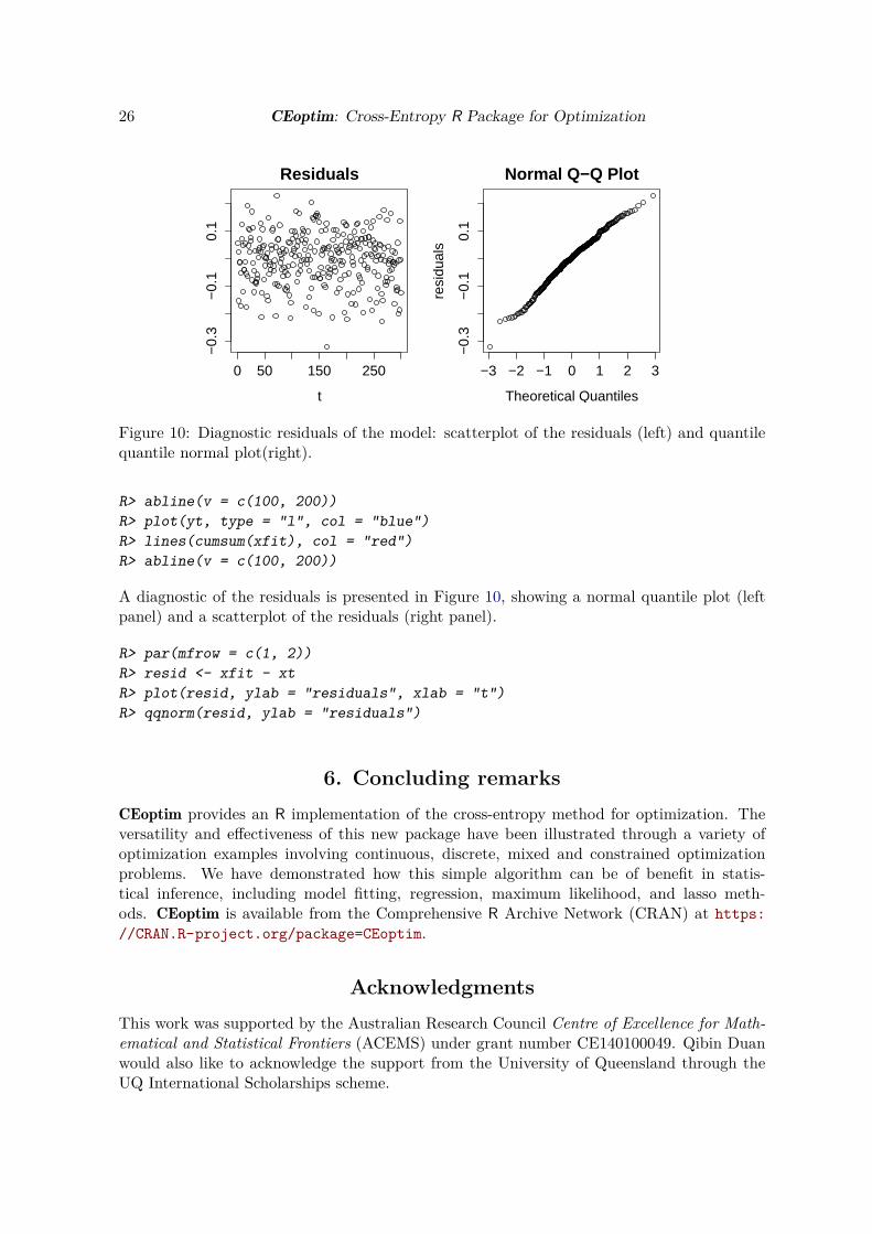
sFigure 10: Diagnostic residuals of the model: scatterplot of the residuals (left) and quantilequantile normal plot(right).
R> abline(v = c(100, 200))R> plot(yt, type = "l", col = "blue")R> lines(cumsum(xfit), col = "red")R> abline(v = c(100, 200))
A diagnostic of the residuals is presented in Figure 10, showing a normal quantile plot (leftpanel) and a scatterplot of the residuals (right panel).
R> par(mfrow = c(1, 2))R> resid <- xfit - xtR> plot(resid, ylab = "residuals", xlab = "t")R> qqnorm(resid, ylab = "residuals")
6. Concluding remarksCEoptim provides an R implementation of the cross-entropy method for optimization. Theversatility and effectiveness of this new package have been illustrated through a variety ofoptimization examples involving continuous, discrete, mixed and constrained optimizationproblems. We have demonstrated how this simple algorithm can be of benefit in statis-tical inference, including model fitting, regression, maximum likelihood, and lasso meth-ods. CEoptim is available from the Comprehensive R Archive Network (CRAN) at https://CRAN.R-project.org/package=CEoptim.
AcknowledgmentsThis work was supported by the Australian Research Council Centre of Excellence for Math-ematical and Statistical Frontiers (ACEMS) under grant number CE140100049. Qibin Duanwould also like to acknowledge the support from the University of Queensland through theUQ International Scholarships scheme.
Journal of Statistical Software 27
References
Alon G, Kroese DP, Raviv T, Rubinstein RY (2005). “Application of the Cross-EntropyMethod to the Buffer Allocation Problem in a Simulation-Based Environment.” The Annalsof Operations Research, 134(1), 137–151. doi:10.1007/s10479-005-5728-8.
Bendtsen C (2012). pso: Particle Swarm Optimization. R package version 1.0.3, URL https://CRAN.R-project.org/package=pso.
Benham T, Duan Q, Kroese DP, Liquet B (2017). CEoptim: Cross-Entropy R Packagefor Optimization. R package version 1.2, URL https://CRAN.R-project.org/package=CEoptim.
Botev ZI, Kroese DP, Rubinstein RY, L’Ecuyer P (2013). “The Cross-Entropy Method forOptimization.” In Handbook of Statistics – Machine Learning: Theory and Applications,volume 31, pp. 35–59. Elsevier. doi:10.1016/b978-0-444-53859-8.00003-5.
Butts CT (2008). “Social Network Analysis with sna.” Journal of Statistical Software, 24(6),1–51. doi:10.18637/jss.v024.i06.
De Boer PT, Kroese DP, Mannor S, Rubinstein RY (2005). “A Tutorial on the Cross-Entropy Method.” The Annals of Operations Research, 134(1), 19–67. doi:10.1007/s10479-005-5724-z.
Duan Q, Kroese DP, Brereton T, Spettl A, Schmidt V (2014). “Inverting Laguerre Tessella-tions.” The Computer Journal, 57(9), 1431–1440.
Friedman J, Hastie T, Tibshirani R (2008). “Regularization Paths for Generalized LinearModels via Coordinate Descent.” Journal of Statistical Software, 33(1), 1–22. doi:10.18637/jss.v033.i01.
Knuth DE (1993). The Stanford GraphBase: A Platform for Combinatorial Computing. ACMPress, Reading.
Kobilarov M (2012). “Cross-Entropy Motion Planning.” The International Journal of RoboticsResearch, 31(7), 855–871. doi:10.1177/0278364912444543.
Kothari RP, Kroese DP (2009). “Optimal Generation Expansion Planning via the Cross-Entropy Method.” In Winter Simulation Conference, pp. 1482–1491.
Kroese DP, Hui KP, Nariai S (2007). “Network Reliability Optimization via the Cross-Entropy Method.” IEEE Transactions on Reliability, 56(2), 275–287. doi:10.1109/tr.2007.895303.
Minka TP (2012). “Estimating a Dirichlet Distribution.” Technical report, Machine In-telligence and Perception Group. URL https://tminka.github.io/papers/dirichlet/minka-dirichlet.pdf.
Mullen KM, Ardia D, Gil DL, Windover D, Cline J (2011). “DEoptim: An R Package forGlobal Optimization by Differential Evolution.” Journal of Statistical Software, 40(6), 1–26.doi:10.18637/jss.v040.i06.
28 CEoptim: Cross-Entropy R Package for Optimization
Nagumo J, Arimoto S, Yoshizawa S (1962). “An Active Pulse Transmission Line SimulatingNerve Axon.” Proceedings of the IRE, 50(10), 2061–2070. doi:10.1109/jrproc.1962.288235.
Ramsay JO, Hooker G, Campbell D, Cao J (2007). “Parameter Estimation for DifferentialEquations: A Generalized Smoothing Approach.” Journal of the Royal Statistical SocietyB, 69(5), 741–796. doi:10.1111/j.1467-9868.2007.00610.x.
R Core Team (2016). R: A Language and Environment for Statistical Computing. R Founda-tion for Statistical Computing, Vienna, Austria. URL https://www.R-project.org/.
Rubinstein RY (1997). “Optimization of Computer Simulation Models with Rare Events.”European Journal of Operational Research, 99(1), 89–112. doi:10.1016/s0377-2217(96)00385-2.
Rubinstein RY (1999). “The Cross-Entropy Method for Combinatorial and Continuous Op-timization.” Methodology and Computing in Applied Probability, 1(2), 127–190. doi:10.1023/a:1010091220143.
Rubinstein RY, Kroese DP (2004). The Cross-Entropy Method: A Unified Approach to Com-binatorial Optimization, Monte-Carlo Simulation and Machine Learning. Springer-Verlag,New York.
Rubinstein RY, Kroese DP (2017). Simulation and the Monte Carlo Method. 3rd edition.John Wiley & Sons, New York.
Sani A, Kroese DP (2008). “Controlling the Number of HIV Infectives in a Mobile Population.”Mathematical Biosciences, 213(2), 103–112. doi:10.1016/j.mbs.2008.03.003.
Soetaert K, Petzoldt T, Setzer RW (2010). “Solving Differential Equations in R: PackagedeSolve.” Journal of Statistical Software, 33(9), 1–25. doi:10.18637/jss.v033.i09.
The MathWorks Inc (2014). MATLAB – The Language of Technical Computing, VersionR2014b. Natick, Massachusetts. URL http://www.mathworks.com/products/matlab/.
Xiang Y, Gubian S, Suomela B, Hoeng J (2013). “Generalized Simulated Annealing forGlobal Optimization: The GenSA Package.” The R Journal, 5(1), 13–28. doi:10.1080/10556780008805777.
Affiliation:Tim Benham, Qibin Duan, Dirk P. KroeseSchool of Mathemathics and PhysicsThe University of QueenslandBrisbane, AustraliaE-mail: [email protected], [email protected], [email protected]

Journal of Statistical Software 29
Benoît LiquetSchool of Mathemathics and PhysicsThe University of QueenslandARC Centre of Excellence for Mathematical and Statistical FrontiersQueensland University of Technology (QUT)Brisbane, AustraliaLaboratoire de Mathématiques et de leurs Applications,Université de Pau et des Pays de l’Adour,UMR CNRS 5142, Pau, FranceE-mail: [email protected] (corresponding author)
Journal of Statistical Software http://www.jstatsoft.org/published by the Foundation for Open Access Statistics http://www.foastat.org/
February 2017, Volume 76, Issue 8 Submitted: 2015-02-27doi:10.18637/jss.v076.i08 Accepted: 2015-11-15