ISSN 2042-2695

CEP Discussion Paper No 1373

September 2015

Loss Aversion on the Phone

Christos Genakos Costas Roumanias Tommaso Valletti

Abstract We analyze consumer switching between mobile tariff plans using consumer-level panel data. Consumers receive reminders from a specialist price-comparison website about the precise amount they could save by switching to alternative plans. We find that the effect on switching of being informed about potential savings is positive and significant. Controlling for savings, we also find that the effect of incurring overage payments is also significant and six times larger in magnitude. Paying an amount that exceeds the recurrent monthly fee weighs more on the switching decision than being informed that one can save that same amount by switching to a less inclusive plan, implying that avoidance of losses motivates switching more than the realization of equal-sized gains. We interpret this as evidence of loss aversion. We are also able to weigh how considerations of risk versus loss aversion affect mobile tariff plan choices: we find that a uniform attitude towards risk in both losses and gains has no significant influence on predicting consumers’ switching, whereas perceiving potential savings as avoidance of losses, rather than as gains, has a strong and positive effect.

Keywords: loss aversion, consumer switching, tariff plans, risk aversion, mobile telephony JEL codes: D03; D12; D81; L96

This paper was produced as part of the Centre’s Growth Programme. The Centre for Economic Performance is financed by the Economic and Social Research Council.

We thank seminar audiences at several universities and conferences for useful comments. We especially thank Stelios Koundouros, founder and CEO of Billmonitor.com, for sharing the data and his industry experience with us. The opinions expressed in this paper and all remaining errors are those of the authors alone.

Christos Genakos, Athens University of Economics and Business and Associate at Centre for Economic Performance, London School of Economics. Costas Roumanias, Athens University of Economics and Business. Tommaso Valletti, Imperial College London, University of Rome “Tor Vergata” & CEPR.

Published by Centre for Economic Performance London School of Economics and Political Science Houghton Street London WC2A 2AE

All rights reserved. No part of this publication may be reproduced, stored in a retrieval system or transmitted in any form or by any means without the prior permission in writing of the publisher nor be issued to the public or circulated in any form other than that in which it is published.

Requests for permission to reproduce any article or part of the Working Paper should be sent to the editor at the above address.

C. Genakos, C. Roumanias and T. Valletti, submitted 2015.

2

1. Introduction

Understanding consumer choice behavior under uncertainty is a central issue across a range

of social sciences. Following Kahneman and Tversky’s (1979) and Tversky and Kahneman’s

(1992) pioneering work, a large literature has shown that individuals evaluate economic

outcomes not only according to an absolute valuation of the outcomes in question, but also

relative to subjective reference points. Loss aversion, one of the pillars of prospect theory,

asserts that losses relative to a reference point are more painful than equal-sized gains are

pleasant. Yet, despite the overwhelming laboratory evidence,5 relatively few field studies

document this phenomenon, and the ones that do involve choices in which risk plays a minor,

even non-existent, role.

In this paper, we present novel evidence that loss aversion plays a pivotal role in explaining

how people select their contracts in the mobile telecommunications industry. We use a new

individual-level panel dataset of approximately 60,000 mobile phone users in the UK

between 2010 and 2012. Consumers in our sample subscribe to monthly plans with a fixed

payment component (the monthly rental) that includes several allowances (for call minutes,

text messages, data usage, etc.). We argue that the monthly rental payment provides a natural

reference point. If a customer exceeds her allowance, she pays extras fees, called overage

fees. This customer could save money by switching to a higher, more inclusive, plan. A

customer could also save money by switching to a lower, less inclusive tariff if her

consumption is systematically lower than her allowance. We conjecture that, in line with loss

aversion, paying more than the reference point is a more “painful” experience and should

prompt consumers to switch with higher probability than they would if they could save the

exact same amount by switching to a lower tariff.6

A unique feature of our data is the way that savings are calculated. In general, people can

make mistakes in predicting their phone usage or have a limited ability to compute the

savings from the many available alternatives, which might generate both biases and inertia. In

our setting, phone users have registered with a specialist mobile comparison website, and

customers’ potential savings are calculated by an optimizing algorithm devised by a company

that is allowed to look into their past bills. Consumers then receive personalized information

5 For an excellent summary of this evidence, see Camerer et al. (2004). 6 Kahneman (2003), in his Nobel acceptance speech, similarly observed: “The familiar observation that out-of-pocket losses are valued much more than opportunity costs is readily explained, if these outcomes are evaluated on different limbs of the value function.”

3

on the exact amount they could save by switching to the best contract for them. In other

words, it can be argued that in our sample, consumers know precisely how much they can

save by switching to a lower- or a higher-tariff plan.

Based on this information, we evaluate the within-person changes affecting the likelihood of

switching contracts over time. We show that potential savings are a significant determinant of

switching. More importantly, and in line with our loss-aversion conjecture, we find that,

controlling for savings, switching is six times more likely if the customer was charged

overage fees.

The case of the mobile phone industry is of particular interest, as mobile phones are

ubiquitous and people spend a considerable amount of money on them.7 Our findings are also

applicable beyond cellular services to many economic settings in which consumers choose

“three-part” tariff contracts that specify fixed fees, allowances, and payments for exceeding

the allowances (e.g., car leases, credit cards, subscription services; see Grubb, forthcoming).

Note that these environments are, almost by definition, uncertain, as there is a random

element in people’s behavior that determines what is ultimately consumed and charged. This

uncertainty brings with it an element of risk.

Placing risk aversion vis-à-vis loss aversion is of economic importance, as, in many real-life

environments, the potential of both gain and loss is most likely to co-exist with risk. In

situations of choice under uncertainty, prospect theory first foregrounded the importance of

loss versus gain, whereas expected utility theory typically assumes a uniform attitude towards

risk. Although a large body of literature has focused on assessing the relevant merits of the

two theories (e.g., Rabin, 2000; Fehr and Göette, 2007), to the best of our knowledge, no one

has attempted to account for both with field data. We believe that this is important, as we do

not see loss aversion and risk aversion as antagonistic, just as we do not necessarily see loss

aversion and traditional expected utility theory as mutually exclusive. In principle, they can

both help us understand the determinants of choice. Given the appropriate data, it becomes an

empirical question to test whether the predictions from either theory are consistent with the

data, as well as the extent to which they can help predict observed behavior. In this study, we

do not assume or impose constraints on our consumers but, rather, allow both risk and loss

aversion to affect their choices.

7 In the UK, mobile revenues have been stable at over £15bn ($23bn) per year over the past decade. This corresponds to about £200 ($300) per year per active subscriber. See Ofcom (2013).

4

Testing for the influence of both, we actually find that risk aversion cannot explain

consumers’ switching, as traditional expected utility theory would suggest, whereas loss

aversion remains strong and significant under all specifications examined. We also find that

individuals seem to be risk-averse in the domain of gains and risk seekers in the domain of

losses: this differential risk attitude, resulting in an S-shaped behavior of their value function,

is consistent with prospect theory.8

Our work is related to a large empirical literature on consumer search and choice behavior.

Five key aspects distinguish our work from earlier studies.9 First, we use actual consumer-

level information from a large sample of consumers in an advanced economy.10

Second, the leading mobile price comparison site in the UK calculates the savings, and each

consumer receives personalized information via email. Thus, in our environment, customers

should suffer significantly less from “comparison frictions,” as in Kling et al. (2012), who

show that simply making information available does not ensure that consumers will use it.

Third, we test for loss aversion in an environment in which uncertainty is not fixed. Existing

work typically establishes an asymmetric attitude between gains and losses either when

choices are riskless (the example of the “endowment effect”)11 or in environments in which

uncertainty is excluded as an explanation of observed behavior because it is held constant

throughout the experiment. For example, Fryer et al. (2012) present evidence of loss aversion

by fixing the mean and variance and exposing subjects to choices between losses and gains in

a field experiment in education. Teachers were shown to have better results when faced with

a compensation program that initially presented them with a bonus that was taken away if

targets were not met (loss) than when facing the same average compensation and same

8 Genesove and Mayer (2001) observe that house market prices are more flexible upward than downward, which implies that sellers’ reservation prices are less flexible downward than buyers’ offers. They suggest that the sellers’ reservation price depends on the purchase price of their house (reference point). Sellers with an expected selling price below the purchase price set a reservation price that is higher than the price set by sellers who do not incur losses. This is also what we find in our data. 9 There is a large body of literature summarizing the main theories of individual decision making in psychology and economics. Rabin (1998), DellaVigna (2009), Barberis (2013), Kőszegi (2014) and Chetty (2015) provide excellent reviews of the evidence in the field. 10 In related work, Jiang (2012) uses survey data from the US, whereas Grubb (2009) and Grubb and Osborne (2015) use data from a student population only. 11 The “endowment effect” is the observation that experimental subjects, who are randomly endowed with a commodity, ask for a selling price that substantially exceeds the buying price of subjects who merely have the possibility to buy the commodity (see, e.g., Kahneman et al., 1990; Knetsch, 1989). List (2003, 2004) questions the robustness of this effect, demonstrating that experienced dealers are much more willing to exchange an initial object they are given for another one of similar value. However, Kőszegi and Rabin (2006) argue that List’s results may be fully consistent with prospect theory, and more recent research tries to explore this hypothesis further (Ericson and Fuster, 2011; Heffetz and List, 2014).

5

variance that awarded them a bonus only if targets were met (gain). Similarly, Pope and

Schweitzer (2011) show that professional golfers react differently to the same shot when they

are under par than when they are over. Although this clearly provides evidence of asymmetric

reaction to loss, golfers over par do not face a more uncertain environment than those under

par, so loss aversion cannot be tested alongside risk aversion. Our environment offers a

natural interpretation of loss-gain asymmetry, and, furthermore, variance can be easily and

naturally measured through bill variability to provide an index for testing risk’s contribution

to consumer choice. In other works, authors have taken stances in favor of one or the other,

while arguing that alternative explanations would not be realistic in the setting they study.

For example, Cohen and Einav (2007) estimate risk aversion in insurance and argue that

alternative preference-based explanations are not relevant in their context, while Ater and

Landsman (2013) study retail banking and base their approach on loss aversion, reasoning

that risk plays a minor, possibly non-existent, role.

Fourth, we analyze a context in which switching can ensure rather large monetary savings. In

related research, Ater and Landsman (2013) analyze customers’ switching decisions after

observing the overcharges on their previously held plans in a retail bank. They find that

customers who incur higher surcharges (losses) have a greater tendency to switch, a finding

that we also share. However, despite the large estimated effect of surcharges, the absolute

monetary value in their case is very small compared to average consumers’ income or

savings. Moreover, their data do not allow them to distinguish between classic risk aversion

and loss aversion: it is possible that customers with risk aversion choose systematically

higher plans than needed and switch more rarely. Most importantly, although Ater and

Landsman (2013) calculate potential savings ex post, it is not likely that customers

themselves know or could easily calculate the level of savings before their switching

decision. So it is possible that customers with overage react to what they perceive as a

savings opportunity, which customers with usage that falls below their allowance cannot

easily detect or calculate. In this, our framework is drastically different. Our customers are

explicitly informed about their potential savings by an expert company that they have chosen

to register with. So they are fully aware of their potential savings when they make their

switching decisions. Asymmetries cannot be attributed to misconstruing overage as a greater

savings opportunity.

Fifth, we study telecoms in a mature phase of the industry. We expect customers in our

sample to have considerable experience in searching and selecting among operators’ tariffs,

6

given that mobile penetration has exceeded 100% of the population since 2004 in the UK,12

and that mobile operators have tried and tested their pricing schemes to optimize profits in a

highly competitive industry.13

In this paper, we concentrate on understanding the determinants of consumer switching. We

do not attempt to evaluate the optimality of consumers’ decisions and refrain from making

welfare claims.14 Therefore, though closely related, our application of behavioral economics

to cellular phones is different from the extant literature on overconfidence and flat-rate bias.15

The remainder of the paper is organized as follows. Section 2 introduces the UK mobile

communications industry and describes the consumer-switching problem. Data are presented

in Section 3, while Section 4 introduces the empirical strategy. Results are discussed in

Section 5, alongside several robustness checks. Section 6 concludes.

2. The industry and the consumer decision process

2.1 Mobile communications in the UK

Mobile communications in the UK are provided by four licensed operators: Vodafone, O2

(owned by Telefonica), Everything Everywhere16 and the latest entrant, Three (owned by

Hutchison). They all provide their services nationally. In 2011 (midway through our sample),

there were 82 million mobile subscribers among a population of 63 million. These

subscribers were split 50:50 between pre-paid (pay-as-you-go) and post-paid (contract)

customers. The latter typically consume and spend more than the former.

12 Hence, we differ, e.g., from Miravete (2002), who considers the early days of the US cellular industry, and

from Jiang (2012), who also uses early data to simulate policies introduced later. 13 Our paper is also related to recent literature that has exploited rich data from cellular companies to analyze a wide range of issues, such as optimal contracts (Miravete, 2002), consumer inertia (Miravete and Palacios-Huerta, 2014), as well as competitive dynamics and the impact of regulation (Economides et al., 2008; Seim and Viard, 2011; Genakos and Valletti, 2011). 14 We have no information on the tariff recommended by the comparison website, and, hence, we cannot evaluate whether customers followed that advice or chose some other tariff. 15 Using cellular contracts, Lambrecht and Skiera (2006), Lambrecht et al. (2007) and Grubb and Osborne (2015) discuss how, in the presence of mistakes related primarily to underusage, the consumers’ bias might be systematic overestimation of demand and could cause a flat-rate bias. Were mistakes due primarily to overusage, the consumers’ bias might be systematic underestimation of demand, consistent, instead, with naive quasi-hyperbolic discounting (DellaVigna and Malmendier, 2004). 16 Everything Everywhere was formed after the 2009 merger between Orange and T-Mobile (owned by Deutsche Telekom).

7

The industry is supervised by a regulator, the Office of Communications (Ofcom). The

regulator controls licensing (spectrum auctions) and a few technical aspects (such as mobile

termination rates and mobile number portability), but, otherwise, the industry is deregulated.

Operators freely set prices to consumers. The four operators have entered into private

agreements with Mobile Virtual Network Operators (MVNOs) to allow them use of their

infrastructure and re-branding of services (e.g., Tesco Mobile and Virgin Mobile). These

MVNOs typically attract pre-paid customers and account for less than 10% of the overall

subscriber numbers (and less in terms of revenues).

Post-paid tariff plans are multi-dimensional. They include a monthly rental, a minimum

contract length, voice and data allowances, and various add-ons and may be bundled with a

handset and various services. Pre-paid tariffs have a simpler structure.

As in other industries, there have been concerns about the complexity of the tariffs and the

ability of consumers to make informed choices. Ofcom, however, has never intervened

directly in any price setting or restricted the types of tariffs that could be offered.17 Instead,

Ofcom has supported the idea that information should let consumers make better choices, as

consumers are more likely to shop around when there is information available with which to

calculate savings from switching tariff plans. The regulator has, therefore, awarded

accreditations to websites that allow consumers to compare phone companies to find the

lowest tariffs. In 2009, Billmonitor.com (henceforth BM), the leading mobile phone price

comparison site in the UK, was the first company to receive such an award for mobile phone

services, and its logo appears on Ofcom’s website.18

Based on Ofcom’s (2013) report, the annual switching between operators (churn rate) varies

between 12% and 14% for the years 2010-2012. There is no publicly available data on

within-operator switching, as this is private information held by operators. In the BM sample,

we observe that some 23% of the customers switch contracts within-operator at least once

annually during the same period. Although the BM sample consists only of post-paid

customers that, on average, consume and spend more, we will demonstrate that it has a very

good geographic spread across the UK and closely matches mobile operators’ market shares

17 In the UK, this has instead occurred in the energy and banking sectors. For price controls in the UK energy sector, see https://www.ofgem.gov.uk/ofgempublications/64003/pricecontrolexplainedmarch13web.pdf. For price controls in the banking sector, see Booth and Davies (2015). 18 http://consumers.ofcom.org.uk/tv-radio/price-comparison/. It is important to note that Ofcom emphasizes the independence of these websites. In the BM case, there is no conflict of interest between the advice that they provide and the choice that consumers make, as the site neither sponsors nor accepts advertising from any mobile provider.

8

and consumer tariff categories, indicating that it is representative of contract customers rather

than prepaid phone customers. Even with this caveat in mind, the high within-operator

switching suggests that this is an important and heretofore underappreciated source of

switching that can be very informative for understanding consumer behavior.

2.2 The consumer decision process

Upon users’ registration with the website, BM attains access to their online bills. BM

downloads past bills, calculates potential savings for the user, 19 and then informs the

consumer of these potential savings. The process is repeated monthly, as shown in Figure 1.

On a typical month t, the bill is obtained on day s of the month. BM logs on to the user’s

mobile operator account and updates the user’s bill history. It uses the updated history to

calculate potential savings, which it then emails and texts to the user. Thus, on day s, the

consumer receives her bill, followed by an email and a text from BM with potential savings

based on her usage history and the current market contract availability. BM also recommends

a new plan to the customer. The consumer decides whether to act on the information (switch

= 1, don’t switch = 0), with no obligation to choose the recommended plan. The decision is

reflected in next month’s (t + 1) bill. On day s of month t + 1, the consumer receives her new

bill. Then, the savings for month t + 1 are calculated and communicated to the consumer,

who then decides whether to stay with her current plan, and so on. Thus, the switch decision,

eventually observed at time t + 1, is based upon usage and savings information collected and

sent to the user at t.

BM allows registration only to residential customers with monthly contracts, who are

typically the high spenders with more complex tariffs. Two features are immediately relevant

for our purposes. First, despite their complexity, all tariffs are advertised as a monthly

payment, with various allowances. The monthly payment becomes a relevant reference point

for the consumer. We call this anticipated and recurrent monthly payment R, though the

19 In order to calculate savings and suitable contracts, BM builds possible future call, text and data usage scenarios for each customer, based on past usage. Using an advanced billing engine, cost is calculated for different possible usages for all available market plans. The plan that minimizes the customer’s expected cost is chosen, controlling for the variance of bills. The cost for the chosen plan is then contrasted with the cost under the consumer’s current plan to obtain savings. All savings recommendations are made with respect to the users’ stated preferences at the time they register (e.g., operator, contract length, handset). To protect the intellectual property of BM, the full details cannot be disclosed.

9

customer may end up paying more than this amount if she exceeds her allowances or uses

add-ons not included in the package. In this case, the actual bill, which we denote by B, is

greater than R. Second, BM calculates the cost of alternative contracts and, given the

expected consumer behavior, picks the cheapest contract for the particular consumer and

informs her about it. If C is the cost of the cheapest contract, as calculated by BM, the

message that BM sends the user should be informative in at least two respects. First, the

customer is directly told the total value of the savings she can make – that is, Savings = B –

C. Second, the customer is prompted to see if there have been fees for extras not included in

in the monthly bundle and if she has exceeded the allowances. This is called “overage” in the

cellular industry and happens when B > R.

In Appendix A, we present snapshots of some key moments of the customer experience with

BM.

3. Data description and summary statistics

For our analysis, we combined four different datasets obtained from BM20 into a single one

with more than 245,000 observations that contain monthly information on 59,772 customers

from July 2010 until September 2012. For each customer-month, we have information on the

current tariff plan (voice, text, data allowance and consumption, plus the tariff cost), the total

bill paid and the calculated savings. 21

Given that the data come from a price comparison website on which consumers freely

register, it is important to examine the representativeness of our sample (see Appendix B for

details). 22 We compare observable characteristics of the BM sample with available

information on UK mobile users. As noted earlier, BM allows only monthly-paying

customers to register, so we do not have information on pay-as-you-go mobile customers.

20 The four datasets are: the accounts dataset, which contains an anonymized account identification code for each customer who registers with BM, together with her codified phone number and current operator; the bills’ dataset, which contains information on the tariff cost, total cost and characteristics of the plan in each month (for example, voice, texts and data allowance); the usage dataset, which contains itemized information of every bill in each month; and the savings dataset, which provides details on the information sent by BM on how much the customer could save by switching to the best available tariff for her. 21 We do not have information on the suggested tariff plan, which is, however, observed by the user. 22 All contracts are single-customer contracts, and we do not observe business contracts – i.e., a single entity

owning multiple phone contracts.

10

First, looking at the geographic dispersion, the distribution of our customers closely matches

that of the UK population in general (Appendix Figure B1).

Second, the operators’ market shares also match quite accurately. The only exceptions are

Everything Everywhere, which is slightly overrepresented in our sample, and Three (the

latest entrant), where we have a smaller market share in our data compared to data available

from the regulator (Appendix Figure B3).

Third, in terms of average revenue per user (ARPU), we have overall higher revenues, which,

of course, can be explained by the fact that we have only post-paid customers. Otherwise, the

ranking of the operators is roughly equivalent (Appendix Figure B5).

Fourth, we have a good representation of customers in different tariff plans. We can compare

our sample with the aggregate information available from Ofcom on the percentage of

customers in each segment. The only category that is underrepresented in our sample is the

lowest tariff plan, which is, perhaps, reasonable given that there is reason to believe that

customers who register with BM are those on larger tariff plans, as they can make bigger

savings (Appendix Figure B6).

Finally, according to Ofcom information, customers in our data send 50 more text messages23

and talk slightly more24 than the average consumer, which also explains the higher ARPU.

Overall, it seems that our sample has a very good geographic coverage of the UK and is in

line with the aggregate market picture of operators and tariffs. The customers in our data

seem to be heavier users, but the overall picture is representative of the post-paid (contract)

segment in the UK.25

3.1 Sample summary statistics

In this section, we highlight some of the most interesting aspects of consumers’ behavior in

our sample, related to savings, overage and switching.

23 Based on Ofcom (2013), the average number of SMS per month was 201, whereas in the BM dataset, customers sent 251. 24 Based on Ofcom (2013), the average minutes per month were 207, whereas they were 235 in the BM dataset. 25 We do not have information concerning the age or mobile experience of customers. When we control for the number of months that we observe each customer in our data, a proxy for contract tenure, the coefficient is not significant, indicating that, at least within our sample, “experience” does not make any difference for savings.

11

Savings

A unique aspect of our data is the savings information calculated by BM. A customer can

save money (positive savings) by switching to either a lower or a higher tariff plan,

depending on her consumption. However, a customer might also have negative savings – that

is, the customer would pay more under the best alternative contract than under her current

contract: no better deal is available. Figure 2 plots the distribution of monthly savings. The

majority of customers have positive savings (73%), with the average being £14 and the

median being £11.

When conditioning savings on some observable characteristics, we find that female

customers have no different savings than men. Likewise, customers throughout the various

UK geographic regions have similar levels of potential savings, reflecting the fact that all

operators are present nationwide (Appendix Figure B2). Additionally, customers across all

operators can save, with some small significant differences among them (Appendix Figure

B4).

An interesting phenomenon is the fact that savings increase significantly as one moves to

higher tariff plans, ranked in different brackets by monthly rentals, following the definition of

Ofcom (Appendix Figure B7).

Overage

Overage is very common: 64% of the customer-months in the BM sample experienced it. If

one looks at the actual difference between the bill and the recurrent tariff cost (B – R), then

the average amount of overspending is £15, with the median being £7. These figures are large

when compared to the average monthly bill, which is £25 in our sample. Overage is common

across genders, different UK regions, and mobile operators. Also interesting is that overage

does not exhibit any particular relationship with different tariff plans and even customers

with negative savings experience it (55% of observations with negative savings have

overage). Overage is very common, not only because it is caused by consuming over and

above one’s current tariff allowance, but also because mobile operators charge their

customers extra for all sorts of other calls and services, such as helplines, premium numbers,

etc.

12

Switching

For data availability reasons, we examine switching only across different tariff plans offered

by the same operator. This is important for two reasons. First, it is relatively easier to switch

within-operator compared to switching across operators. Customers can change tariffs with

the same provider without paying penalties if they switch prior to the expiry of the contract.

Thus, we can be less worried about contractual clauses that we do not observe. Second,

within-operator switching is an important source of switching in the mobile industry – as

reported earlier, in our data, 23% of customers switch within-operator annually. Hence, this

setting is ideal for unraveling frequent consumer choices, though the limitation is that we

cannot say much about industry-wide competitive effects.

The average in-sample probability of switching is 0.080 per month, with women switching

more often than men (0.083 vs 0.077, p-value = 0.0002). Switching is equally distributed

across the UK.

Looking at the savings distribution (Figure 3), switchers (before switching) have higher

savings than non-switchers (£9.3 vs £7.3, p-value = 0.000), and their distribution also has a

fatter right tail. So savings seem to be one of the factors triggering the decision to switch.

Finally, it is worth noting that consumers who had overage on their last bill are also more

likely to switch (0.083 vs. 0.075, p-value = 0.000), indicating that overage might also play a

role in switching behavior. Table 1 reports some key sample summary statistics.26

4. Empirical framework

To analyze consumer switching behavior, we use the following econometric framework:

�������ℎ��� �� = β� + β�Overage����� + β�Savings����� + d� + d� + "��. (1)

26 Due to the use of lagged values in our estimation framework, we lose the first observation of each consumer, as well as a number of consumers who register for only one month.

13

The switching probability for individual i at month t depends on two critical pieces of

information retrieved at time t – 1 from BM: Overage is a binary variable indicating whether

the total bill was higher than the tariff reference cost in a given month (Overage = 1(B, R),

where 1(·) is an indicator function taking the value of 1 if B > R, and zero otherwise); and

Savings is the monthly savings calculated by BM and communicated to the customer. Notice

that we correct for unobserved heterogeneity by extensively controlling for fixed effects: #�

captures customer fixed effects, while #�represents time (joint month-year) fixed effects.

Thus, we control for unobserved differences across customers and unobserved time trends

and shocks. Finally, "�� is the error term that captures all unobserved determinants of the

switching behavior. Our main interest is in the parameter $�that describes the impact of

overspending last month on the probability of switching now, controlling for the amount that

could be saved.

We estimate (1) using mainly a linear probability specification and calculate the standard

errors based on a generalized White-like formula, allowing for individual-level clustered

heteroskedasticity and autocorrelation (Bertrand et al., 2004). We also estimate a simple and

a conditional (fixed effects) logit model. Although such a model is better suited to the binary

dependent variable, it is not ideal for our purposes, as the more appropriate FE logit model

can be estimated only on a subsample of individuals with variation in the switching variable –

i.e., those who switch at least once during the period in which we observe them. This is a

nonrepresentative sample and would overestimate the true marginal effect of the independent

variables. We provide these results to show the qualitative robustness of our results.

In addition, we also use a proportional hazard model (PHM) for the duration between the

time a consumer registers with BM and the time of tariff switching. We estimate (1) utilizing

a semiparametric estimation procedure that allows for time-varying independent variables

(Cox, 1972). According to the Cox PHM, the hazard function is decomposed into two

multiplicative components: ℎ���, &� = ℎ��� × (� , where (� ≡ exp�$′&� . The ℎ��� is the

baseline hazard function that models the dynamics of the probability of switching (hazard

rate) over time; &� is a vector of individual characteristics, and β is a vector of regression

coefficients that includes the intercept; (� scales the baseline hazard proportionally to reflect

the effect of the covariates based on the underlying heterogeneity of consumers. The main

14

advantage of the PHM is that it accounts for censoring27 and is flexible enough to allow for

both time-invariant (e.g., mobile operator) and time-varying control variables (e.g., savings).

5. Results

The main regression results are reported in Tables 2 and 3. Starting with Table 2, when

considered individually, both overage and savings are important in determining a switching

decision (columns 1 and 3, respectively). This result is robust to controlling for time and

individual fixed effects (columns 2 and 4, respectively), and the coefficients actually

increase, indicating that unobserved individual or common factors are biasing the initial

estimates downward.

Column 5 reports the results of the full specification when both overage and savings are

included in the regression. Although we control for savings, overage still has a large and

statistically significant coefficient. Interestingly enough, both variables retain their previously

estimated magnitudes, indicating that the processes of savings and overage are orthogonal to

each other. More importantly, the economic impact of overage is stronger than that of

savings. A £10 monthly savings increases the expected probability of switching by only

0.23%, whereas if a customer’s monthly bill is higher than her tariff, the probability of

switching increases almost sixfold, to 1.32%.

Results are qualitatively unchanged when we use a logit model given the binary nature of the

dependent variable. Column 6 reports the estimated coefficients and column 7 the odds ratios.

Both estimated coefficients are positive and significant, but a one-pound increase in savings

increases the odds of switching by 0.6%, whereas overage increases the odds by 7.8%.28

Finally, the last two columns present the estimated coefficient of the switching hazard model.

Again, we find that both overage and savings significantly increase the probability of

switching (column 8), where an additional pound of savings increases the hazard of switching

by 0.3%, whereas overage increases the hazard of switching by 9% (column 9).

27 Both right censoring since our sample stops at September 2012 and left censoring since consumers join BM at different points in time. 28 Results using a conditional (individual fixed effects) logit model are even stronger: a one-pound increase in savings increases the odds of switching by 0.8%, whereas overage increases the odds by 18.3%. If we control for individual fixed effects, the logit approach takes into consideration only the customers who experience switching, so it restricts the sample in such a way that it is not comparable with the other regressions. For this reason, Table 2, column 6 reports the results without individual consumer fixed-effects.

15

Hence, results from all different estimation models lead to interesting insights regarding

customer switching among plans. Our findings suggest that, if a consumer is reminded that

her plan is suboptimal – that is, if she could save by switching to another tariff – then the

higher the savings, the more likely it is that the customer will switch.29 This is not particularly

controversial and follows from basic economic reasoning. More intriguing, though, is that

whether a customer has experienced overage payments, over and above savings, also matters

considerably. These customers are also more likely to switch to new tariff plans.

Our results are, therefore, potentially supportive of loss aversion or, more generally, about

mental accounting theories, which occur when individuals group expenditures into mental

accounts and do not treat money as fungible across categories. In our setting, customers treat

fixed monthly payments and overage payments as separate mental accounts, which are

associated with different levels of utility. Customers construct reference points based on such

monthly fees and distinguish between within-budget savings and overage losses. We find that

customers prefer avoiding losses to obtaining gains – indeed, the central prediction of the

theory of loss aversion.

Apart from confirming an asymmetric attitude towards gains and losses, the data also allow

us to test two other key aspects of the way consumers choose. First, we test how loss aversion

fares when considered together with risk aversion in explaining consumer behavior. We do so

because the variability in a consumer’s bill is readily calculable, so including variability as an

explanatory variable tests its contribution to her choice. Second, we test whether there is an

asymmetric attitude towards risk in the domain of gains versus the domain of losses, another

key feature of prospect theory.

To test the extent to which risk aversion might be a factor driving the observed behavior of

mobile telephony customers, we introduce a measure of the variability of payments that is a

good proxy for the importance of fluctuations in payments. More specifically, we construct a

new variable, Bill Variance, which is the variance of the last three bills of a given customer.30

This variable then becomes an additional control in our main equation. Table 3 reports the

29 Consumers switch to both higher and lower tariffs. Of those switching, approximately 55% switch to a lower tariff plan, whereas 45% switch to a higher tariff plan. 30 Denote the monthly bill as -�� . Then, we calculate the average of the last three months,

./ = �-���0 + -���� + -���� 3⁄ , and, hence, the Bill Variance is equal to

34��� = [�-���0 − ./ � + �-���� − ./ � + �-���� − ./ �] 3⁄ .

16

results:31 column 1 estimates a simple OLS regression to test the effect of variance on

switching. The coefficient of variance is not statistically significant. Column 2 repeats the

exercise, controlling for consumer and year-month fixed effects. Variance is now negatively

associated with switching, implying that consumers exhibit an appetite for variance (they

tend to change contracts with higher variability more rarely).32 Column 3 examines the effect

of overage and savings on switching for the same customer-months. The results obtained in

Table 2 remain unchanged.

Having separately examined the effect of overage and variance on switching, we now include

both in column 4. The effects of overage and savings remain unaffected; they are still highly

significant and positive. The effect of variance, however, is no longer significant, implying

that variance cannot account for the observed customer switching. Bill variance is not

statistically significant, and does not change previous results in any significant way. While, in

principle, both loss aversion and risk aversion could play a joint role in a switching decision,

we do not find a role for risk aversion, just for overage payments.

Interestingly, although bill variance is not statistically significant, its interaction with overage

is (column 5). Customers with overage switch significantly less as their bill variance

increases. Hence, consumers in our sample exhibit a risk-loving attitude in the domain of

losses (remember that, for overage customers, the bill exceeds their contract tariff and is

experienced as loss relative to the reference point). On the contrary, customers with no

overage are risk-averse, as they switch more often as variance increases. This is in line with

the familiar S-shaped value function from prospect theory, whereby individuals are risk-

averse in the domain of gains and risk-loving in losses.

5.1 Alternative interpretations and robustness

In this section, we test the robustness of our results in relation to alternative interpretations of

our findings and to measurement and econometric modeling issues.

31 Due to the lagged three-month moving average calculation, we lose some 74,192 customer-month observations. 32 As we explain later, consumers exhibit risk aversion in the domain of gains but an appetite for risk in the domain of losses. When considering how risk affects switching uniformly (that is, in both domains), the latter effect seems to dominate.

17

1. Sample selection due to risk aversion. Loss aversion coexists with uncertainty in our

environment. Overage payments can be seen as unexpected payments that customers try to

avoid. Although we find that bill variance does not affect the probability of switching, in such

an uncertain environment, the degree of risk aversion may still be a factor that could drive the

results in a different way: risk-averse customers may select over-inclusive plans to avoid

fluctuations in their payments. If the information about overage is related to such

fluctuations, these customers then may also be more likely to switch, other things equal.

To investigate this, we divide the sample among small (0 <savings ≤ 3), medium (3 < savings

≤ 11), and large savings (11 < savings ≤ 35).33 Customers that fall in the small savings

bracket are actually very good at predicting their behavior and do not select large buffers

(otherwise, BM would also find large savings for them). Those who have large savings may,

instead, choose large buffers because of aversion to risk. Yet, as columns 1, 2 and 3 of Table

4 indicate, overage is always significant for all these customers, even though they may differ

in several other ways. Results in column 1 are particularly telling: customers with very small

savings do not react to the information that they have some small potential savings.

Nevertheless, once they are informed about overage, even these customers switch contracts

with a higher probability.34 Comparing columns 1, 2 and 3, we note that the magnitude of

overage decreases as savings increase. At the same time, the coefficient of savings is not

significant for those who have small potential savings (indicating that these customers are,

indeed, making cost-efficient choices); however, it is positive and very significant for the

medium bracket and positive and significant, but smaller in size, for the large savings

bracket.35 Hence, as savings increase, loss aversion continues to play a significant, role but

the magnitude of its effect is smaller than that of savings.

2. Overage intensity. Next, we look again at the magnitude of overage. Specifically, we

consider the actual amount by which a bill is higher than the monthly reference tariff, and we

split the overage observations above and below the median. Table 4, column 4 shows that the

higher the overage, the more likely it is that the consumer will switch, while still controlling

33 Cut-off points correspond to the 10th and 90th percentiles of the savings distribution. Results are robust to alternative cut-off specifications. 34 For customers with small savings, consumption matches their chosen plans closely. Small consumption shocks (positive or negative) can push them either above or below their allowances, so overage in this case can be thought of as quasi-randomly allocated across these consumers. Results are very similar if we use a symmetric savings range of -3 < savings ≤ 3. 35 The coefficient on savings increases in magnitude, compared to the main results in Table 2 for the overall sample since we now condition on positive savings.

18

for the magnitude of savings. This seems to indicate that it is not just overage, but also its

magnitude, that play an important role in pushing consumers to switch. The higher the

“shock” associated with overage, the more likely consumers will be to switch to a different

tariff.

3. Contract constraints. Recall that, when consumers register in BM, they are asked to

express their preferences related to the operator that they want BM to search, as well as the

features they are interested in (e.g., a special handset). If a consumer does not select anything,

then BM looks at the universe of available tariffs. Switching between operators can be more

difficult than switching within an operator, as there may be additional costs involved. In

Table 4, column 5, we select consumers who explicitly include their current operator in their

search. As one can see from the number of observations, the vast majority include their

current operator, so savings must be informative. The results clearly do not change. In

column 6, we adopt a more conservative approach and restrict the analysis to those customers

who select only their current operator. In this case, savings must indicate that the best

alternative contract is with their operator and, hence, must be much more informative. Even

with this restriction, the results still hold.

4. Placebo test: negative savings. As a placebo test, we also examine the behavior of

consumers with negative savings. These customers currently have plans with very good

tariffs since BM cannot find cheaper alternatives. However, even these consumers can

experience an overage (55% of the observations of customers with negative savings have

experienced overage), as a total bill is very often the consequence of various extra charges

unrelated to the tariff bundle. But these customers, precisely because their savings are

negative, should not be triggered to take a closer look at their bills, and, as a result, they do

not notice overage. Hence, we would not expect these customers to react either to their

savings or to their overage information. In Table 4, column 7, we find that both coefficients

are not statistically significant.

5. Differences in reactions. Another possible interpretation of our findings is that consumers

who over-consume behave differently than those who under-consume. In particular, one

could argue that consumers who over-consume and experience overage can respond only by

adjusting their tariff, whereas consumers who under-consume can adjust either their

consumption or their tariff. Hence, probabilistically, consumers with no overage are less

likely to switch. We find this explanation unappealing for three reasons. First, there is no

19

clear a priori reason why consumer who under-consume can adjust their consumption more

easily than consumers who over-consume. In principle, both can alter their calling behavior

when they receive the relevant information from BM. Second, for those consumers in the

small savings bracket that we analyzed earlier (Table 4, column 1), the differences between

under- and over-consumers are very small, yet overage continues to play a significant role.

Third, the argument above would imply that since most of the switchers are over-consumers,

the direction of the switching should be for people to increase their tariffs. However, what we

observe is that 58% of the consumers who switch choose a lower tariff, while the remaining

42% switch up, which, again, cannot be reconciled with the above argument. This holds true

also for consumers in the small savings bracket, (50% switch up and 50% switch down),

showing once again that risk aversion alone cannot explain switching behavior.

6. Learning. Finally, a variant of the above argument is that consumers learn about their

optimal bundle by starting with a low tariff plan that they subsequently increase. Thus, the

positive coefficient on overage actually captures the consumer’s learning process and not loss

aversion. We also find this explanation unconvincing in explaining switching. First, we study

UK consumers’ behavior in a mature phase of the telecoms industry. Hence, although we do

not have information on their age, it is highly unlikely that all these customers are first-time

users, unaware of their needs and consumption pattern. Second, if the learning hypothesis

were true, then we would expect the direction of switching to be, on average, upwards, and

this increase to be more evident the lower the tariff category. However, as we argued earlier,

consumers switch to lower tariffs, on average (58% vs 42%), and this tendency actually

increases as we move to lower tariff categories (see Figure A1 in the Appendix).

Next, we consider alternative econometric specifications and also experiment with alternative

measures for some of the key variables. First, controlling for Bill Variance does not alter any

of the previous results, irrespective of the estimation method or sample selected. In Table 3,

column 4, we showed that the coefficient on Bill Variance was not statistically significant

and did not affect the size and statistical significance of overage or savings. This continues to

be the case, even if we apply the logit model or the Cox PHM as alternative estimation

methods (Table A1, columns 1-4). Moreover, controlling for Bill Variance does not alter the

results on the saving brackets of Table 4, columns 1-3. Using the same framework, but now

20

controlling for Bill Variance, provides qualitatively very similar results (Table A1, columns

5-7).

Second, one could argue that if there is measurement error in calculating savings, then their

coefficient would be biased. Similarly, including just last months’ savings may be a more

noisy measure of the true potential savings a customer could achieve. To alleviate these

concerns, we recalculate savings for each customer using a moving average of her last three

months and re-run our baseline results from Table 2. None of our previous results changes in

any fundamental way, while the impact of overage increases slightly (Table A2).

Third, we also experiment by calculating an alternative measure of variance based on

savings. Savings measure consumption variability and, as such, it might be useful to capture

fluctuations in calling behavior. Estimated results are very similar to those previously

obtained (Table A3 replicates the analysis in Table 3).

The picture that emerges from this evidence is one in which customers respond, possibly

sequentially, to the information received from BM. If the message says that the customer is

already on a plan with a good tariff (negative savings), the customer does not have any

incentives to look deeper into her consumption pattern, and she stops there. If, instead, the

customer receives notice that savings are possible, then she is inclined to look much closer at

her behavior and at the contract. This is when she learns about overage, on top of savings,

which then initiates the switching patterns that we described above. The consumer perceives

overage as a loss, irrespective of the savings, and, thus, is much more likely to switch

contracts.

Our results support prospect theory: we found loss aversion to be significant in determining

consumers’ choice to change plans, but we did not find bill variance to be a determinant of

their choice. Consumers who could reduce losses by a certain amount relative to their salient

point (monthly tariff) changed plans significantly more than consumers who could improve

(gain) by the same amount without having experienced overage. We have established that the

asymmetry between losses and gains can explain observed consumer behavior but that a

uniform attitude towards risk in both losses and gains (an assumption central to expected

utility theory) cannot explain customers’ switching. Consumers’ attitude towards risk was

found to be in line with prospect theory: our consumers exhibit an appetite for risk (bill

variance) when they are in the loss (overage) domain.

21

6. Conclusions

We have conducted an assessment of consumer behavior using individual data from UK

mobile operators collected by a price comparison website. We showed that consumers who

receive reminders about possible savings do respond and switch tariff plans. More

interestingly, we also discussed how consumers employ their monthly fixed payment as a

reference point in their choices. When they spend above this reference point, the resulting

overage payment induces considerable switching. This central finding is very much in line

with the Loss Aversion model of Kahneman and Tversky (1979) and is robust to several

alternative interpretations and specifications.

We were also able to weigh how both risk and loss-aversion considerations affect choices in

mobile telephony in a modern western economy: this is a high-stake industry affecting the

majority of the population everywhere in the world. We find that risk aversion cannot explain

consumers’ switching, while loss aversion plays an important role.

Our results put the use of price-comparison sites in a new light. Regulators and competition

authorities worldwide oversee price accreditation schemes for third-party price-comparison

sites covering several industries – in addition to mobile phones – that still exhibit

considerable uncertainty in patterns of consumption over time (e.g., banking, credit cards and

insurance). The aim of these schemes is to increase consumer confidence about how to find

the best price for the service they wish to purchase, and to increase market transparency by

providing or facilitating expert guidance. Thaler and Sunstein (2008) propose the RECAP

(Record, Evaluate, and Compare Alternative Prices) regulation that would require firms to let

customers share their usage and billing data with third parties, such as BM, which could, in

turn, provide unbiased advice about whether to switch to a competing provider.36

The emphasis of these proposals is almost invariably on savings – e.g., finding the most cost-

effective tariff given a certain consumer profile. While this information is certainly useful for

choice, we also show that savings are only a part of the story, and possibly a minor one.

Hence, we introduce a note of caution on expert advisers that is different from any conflict-

of-interest consideration (Inderst and Ottaviani, 2012) or from cases in which nudging may

have adverse market equilibrium effects (Duarte and Hastings, 2012; Handel, 2013). We

suggest that regulators hoping to rely on price-comparison engines to discipline market prices

36 Without implying that nudging is always welfare-increasing

22

using shared data should first investigate what giving good advice means in a context with

loss aversion. Consumers also switch for behavioral reasons that have little to do with

savings, but that still could be consistent with optimal individual behavior.

In this paper, we have limited our analysis to the positive implications of behavioral

economics – namely, on predicting switching behavior in the presence of loss aversion.

Understanding the effect on social welfare is equally important. In particular, consumer

switching is central to any competitive assessment of an industry. Developing a non-

paternalistic method of welfare analysis in behavioral models is, however, a challenge.

Following Chetty (2015), one possibility is to use revealed preferences in an environment in

which agents are known to maximize their “experienced” utility (their actual well-being as a

function of choices), which may differ from their “decision” utility (the objective to be

maximized when making a choice).37 The approach used in our setting is that the amount of

savings is calculated mechanically by an optimizing algorithm; thus, most behavioral biases

should vanish or at least be kept to a minimum. The fact that we still find a considerable role

played by overage implies that loss aversion is of the utmost importance directly in the

experienced utility and must be accounted for in any welfare assessment.

37 An alternative approach is to follow structural modeling that specifies and estimates the structural parameters of a behavioral model. Grubb and Osborne (2015) follow this line to discuss the recent “nudge” adopted by the FCC (the US telecom regulator) of requiring bill-shock alerts for mobile phones (text messages warning when allowances of minutes, texts, or data are reached). They show that providing bill-shock alerts to compensate for consumer inattention can reduce consumer and total welfare because, most likely, firms will adjust their pricing schedule by reducing overage fees and increasing fixed fees.

23

References

Ater, Itai, and Vardit Landsman. 2013. “Do Customers Learn From Experience? Evidence From Retail Banking.” Management Science 59(9): 2019–35.

Barberis, Nicholas C. 2013. “Thirty Years of Prospect Theory in Economics: a Review and Assessment.” Journal of Economic Perspectives 27(1): 173–96.

Bertrand, Marianne, Esther Duflo, and Sendhil Mullainathan. 2004. “How Much Should We Trust Differences-in-Differences Estimates?” Quarterly Journal of Economics 119 (1): 249–275.

Booth, Philip, and Stephen Davies. 2015. “Price Ceilings in Financial Markets,” in Coyne, Christopher and Rachel Colyne (Eds.). Flaws and Ceilings: Price Controls and the

Damage they Cause. Institute of Economic Affairs, London.

Camerer, Colin, George Loewenstein, and Matthew Rabin. 2004. Advances in Behavioral

Economics. Princeton University Press, Princeton.

Chetty, Raj. 2015. “Behavioral Economics and Public Policy: A Pragmatic Perspective.” American Economic Review Papers and Proceedings (forthcoming).

Cohen, Alma, and Liran Einav. 2007. “Estimating Risk Preferences From Deductible Choice.” American Economic Review 97(3): 745–788.

Cox, D R. 1972. “Regression Models and Life Tables.” Journal of the Royal Statistical

Society 34(2): 187–220.

DellaVigna, Stefano. 2009. “Psychology and Economics: Evidence From the Field.” Journal

of Economic Literature 47(2): 315–72.

DellaVigna, Stefano, and Ulrike Malmendier. 2004. “Contract Design and Self-Control: Theory and Evidence.” Quarterly Journal of Economics 119 (2): 353–402.

Duarte, Fabian, and Justine S. Hastings. 2012. “Fettered Consumers and Sophisticated Firms: Evidence from Mexico's Privatized Social Security Market.” NBER Working Paper 18582.

Economides, Nicholas, Katja Seim, and V Brian Viard. 2008. “Quantifying the Benefits of Entry Into Local Phone Service.” RAND Journal of Economics 39(3): 699–730.

Ericson, Keith M. Marzilli, and Andreas Fuster (2011) “Expectations as Endowments: Evidence on Reference-Dependent Preferences from Exchange and Valuation Experiments. ” Quarterly Journal of Economics 126(4):1879–1907.

Fehr, Ernst, and Lorenz Götte. 2007. “Do Workers Work More if Wages Are High.” American Economic Review 97(1): 298–317.

Fryer, Roland G, Jr., Steven D. Levitt, John List, and Sally Sadoff. 2012. “Enhancing the Efficacy of Teacher Incentives Through Loss Aversion.” NBER Working Paper 18237.

Genakos, Christos, and Tommaso Valletti. 2011. “Testing the ‘Waterbed’ Effect in Mobile

24

Telephony.” Journal of the European Economic Association 9(6): 1114–42.

Genesove, David, and Christopher Mayer. 2001. “Loss Aversion and Seller Behavior: Evidence From the Housing Market.” Quarterly Journal of Economics, 116(4): 1233–60.

Grubb, Michael D. 2009. “Selling to Overconfident Consumers.” American Economic Review 99(5): 1770–1807.

Grubb, Michael D. 2015. “Overconfident Consumers in the Marketplace.” Journal of

Economic Perspectives (forthcoming).

Grubb, Michael D, and Matthew Osborne. 2015. “Cellular Service Demand: Biased Beliefs, Learning, and Bill Shock.” American Economic Review 105(1): 234–71.

Handel, Benjamin R. 2013. “Adverse Selection and Inertia in Health Insurance Markets: When Nudging Hurts.” American Economic Review 103(7): 2643–82.

Heffetz, Ori, and John A. List. 2014. “Is the Endowment Effect an Expectations Effect?” Journal of the European Economic Association 12(5): 1396–1422.[Now published, title also changed]

Jiang, Lai. 2012. “The Welfare Effects of ‘Bill Shock’ Regulation in Mobile Telecommunication Markets.” Working Paper.

Kahneman, Daniel. 2003. “Maps of Bounded Rationality: Psychology for Behavioral Economics.” American Economic Review, 93(5): 1449–1475.

Kahneman, Daniel, and Amos Tversky. 1979. “Prospect Theory: an Analysis of Decision Under Risk.” Econometrica 47(2): 263–292.

Kahneman, Daniel, Jack L. Knetsch, and Richard H. Thaler. 1990. “Experimental Tests of the Endowment Effect and the Coase Theorem.” Journal of Political Economy 98(6): 1325–1348.

Kling, Jeffrey R., Sendhil Mullainathan, Eldar Shafir, Lee C. Vermeulen, and Marian V. Wrobel. 2012. “Comparison Friction: Experimental Evidence From Medicare Drug Plans.” Quarterly Journal of Economics 127(1): 199–235.

Knetsch, Jack L. 1989. “The Endowment Effect and Evidence of Nonreversible Indifference Curves.” American Economic Review 79(5): 1277–1284.

Kőszegi, Botond. 2014. “Behavioral Contract Theory.” Journal of Economic Literature 52(4): 1075–1118.

Kőszegi, Botond, and Matthew Rabin. 2014. “A Model of Reference-Dependent Preferences.” Quarterly Journal of Economics 121(4): 1133–65.

Inderst, Roman, and Marco Ottaviani. 2012. “How (not) to pay for advice: A framework for consumer financial protection.” Journal of Financial Economics 105(2): 393–411.

Lambrecht, Anja, and Bernd Skiera. 2006. “Paying Too Much and Being Happy About It: Existence, Causes, and Consequences of Tariff-Choice Biases.” Journal of Marketing

25

Research 43(2): 212–23.

Lambrecht, Anja, Katja Seim, and Bernd Skiera. 2007. “Does Uncertainty Matter? Consumer Behavior Under Three-Part Tariffs.” Marketing Science 26(5): 698–710.

List, John. 2003. “Does Market Experience Eliminate Market Anomalies?” Quarterly

Journal of Economics 118(1): 41–71.

List, John. 2004. “Neoclassical Theory versus Prospect Theory: Evidence from the Marketplace. ” Econometrica 72(2): 615–25.

Miravete, Eugenio J. 2002. “Estimating Demand for Local Telephone Service with Asymmetric Information and Optional Calling Plans.” The Review of Economic Studies 69(4): 943–71.

Miravete, Eugenio J, and Ignacio Palacios-Huerta. 2014. “Consumer Inertia, Choice Dependence and Learning From Experience in a Repeated Decision Problem.” Review of

Economics and Statistics 96(3): 524–537.

Ofcom. 2013. Communications Market Report 2013. Office of Communications, London.

Pope, Devin G, and Maurice E Schweitzer. 2011. “Is Tiger Woods Loss Averse? Persistent Bias in the Face of Experience, Competition, and High Stakes.” American Economic

Review 101(1): 129–57.

Rabin, Matthew. 1998. “Psychology and Economics.” Journal of Economic Literature 36(1): 11–46.

Rabin, Matthew. 2000. “Risk Aversion and Expected‐Utility Theory: a Calibration Theorem.” Econometrica 68(5): 1281–92.

Seim, Katja, and V Brian Viard. 2011. “The Effect of Market Structure on Cellular Technology Adoption and Pricing.” American Economic Journal: Microeconomics 3(2): 221–51.

Thaler, Richard, and Cass Sunstein. 2008. Nudge: Improving Decisions about Health,

Wealth, and Happiness. Yale University Press, New Haven.

Tversky, Amos, and Daniel Kahneman. 1992. “Advances in Prospect Theory: Cumulative Representation of Uncertainty.” Journal of Risk and Uncertainty 5(4): 297–323.

26

Appendix A – The consumer experience with Billmonitor.com

In this annex, we present in various screen shots the consumer experience of registering and

using BM’s services. BM was created to provide impartial information and to help monthly

paid mobile phone customers to choose contract that is best for them. BM was first accredited

by Ofcom in 2009 and still receives accreditation (Figure A1). To safeguard its impartiality,

BM neither receives advertising from any mobile operator nor allows for any kind of

promotions on its website. It simply collects all available contract information from all UK

mobile operators and tries to match each consumer’s consumption pattern with the best

available tariff.

FIGURE A1: BM’s OFCOM RE-ACCREDITATION

When a user visits the BM webpage, she is prompted to register in order to have her bills

analyzed and to determine “exactly the right mobile contract” for her (Figure A2).

27

FIGURE A2: BM’s HOME PAGE

If she chooses to have the BM engine analyze her bills, she is led to a page asking for her

details (mobile operator, phone number, username and password and email), as shown in

Figure A3.

FIGURE A3: BM’s ANALYSIS PAGE

During the analysis of her bill, she is presented with a screen that informs her that BM

searches through all possible contract combinations to find the “right” contract for her

(Figure A4).

28

FIGURE A4: BM’s CALCULATION SCREEN

Upon analysis of her bill, the user receives an email informing her of potential savings. This

email is repeated monthly, the day after her bill is issued, as described in Figure 1 in the main

text. Figure A5 shows an example of such an email.

FIGURE A5: EMAIL SENT TO USERS INFORMING THEM OF POTENTIAL SAVINGS

29

Appendix B – Representativeness of the sample and summary statistics

In this annex, we discuss the representativeness of our sample and also provide some initial

statistics on savings within our sample.

Figure B1 compares the geographic distribution of the population residing in the UK (ONS,

2011 census) with the customers registered with BM. As the figure shows, BM customers are

well spread across the UK and match the actual population spread closely.

FIGURE B1: POPULATION DISTRIBUTION ACROSS UK REGIONS

Notes: The graph above compares the percentage population distribution across regions in the UK and in the BM data. Source: UK population distribution based on 2011 census, Office for National Statistics. BM population distribution based on the data provided by BM.

In all these different regions, consumers can realize savings by switching to different tariffs

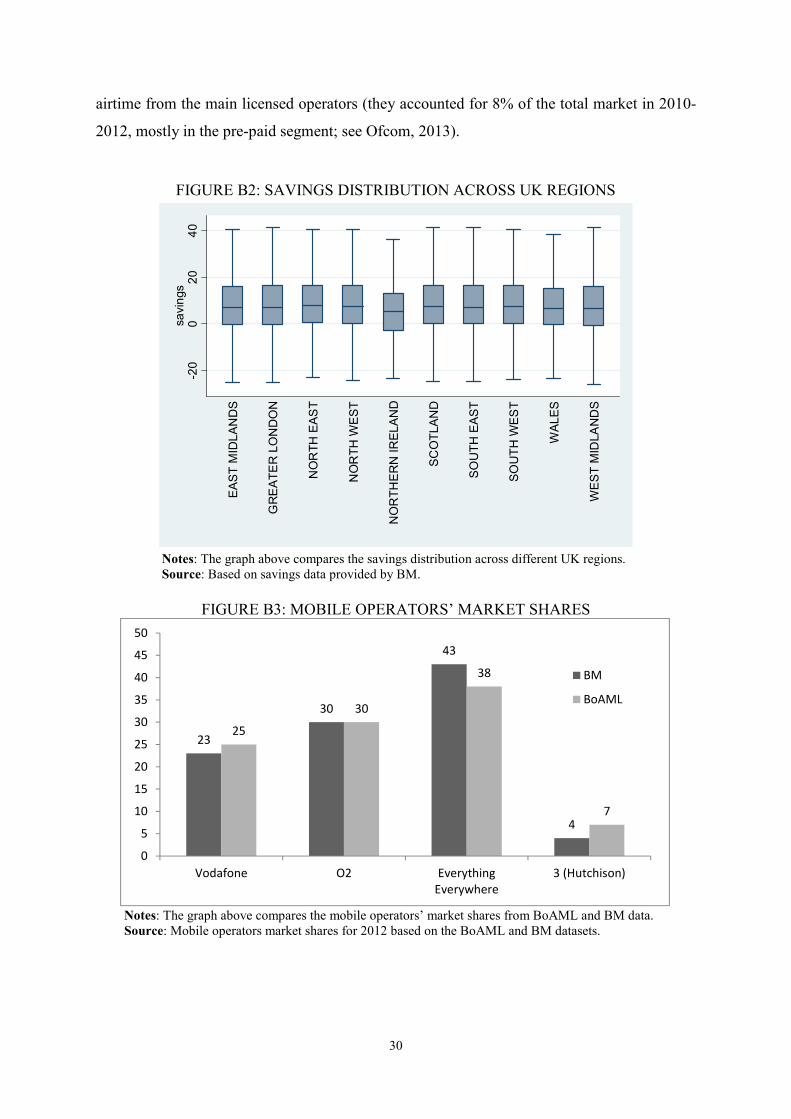
(Figure B2). Savings are, on average, positive across all regions, with the highest median

savings in the North East (£7.2) and the lowest in Northern Ireland (£4).

Figure B3 compares mobile operators’ market shares in BM data with aggregate market

information from the Bank of America Merrill Lynch (BoAML) dataset for 2012. Aggregate

market shares are well tracked in the BM data, with the exception of Everything Everywhere

(the merged entity of T-Mobile and Orange) that is slightly overrepresented and Three

(Hutchison), which is slightly underrepresented. These discrepancies can be attributed to the

fact that aggregate market shares also allocate to the licensed operators market shares of

MVNOs (Mobile Virtual Network Operators) that do not have a spectrum license but rent

12

16

7

13

2

7

16

10

6

109

16

5

13

4

10

17

10

6

11

0

2

4

6

8

10

12

14

16

18 BM

UK

30

airtime from the main licensed operators (they accounted for 8% of the total market in 2010-

2012, mostly in the pre-paid segment; see Ofcom, 2013).

FIGURE B2: SAVINGS DISTRIBUTION ACROSS UK REGIONS

Notes: The graph above compares the savings distribution across different UK regions. Source: Based on savings data provided by BM.

FIGURE B3: MOBILE OPERATORS’ MARKET SHARES

Notes: The graph above compares the mobile operators’ market shares from BoAML and BM data. Source: Mobile operators market shares for 2012 based on the BoAML and BM datasets.

-20

020

40

savings

EAST MIDLANDS

GREATER LONDON

NORTH EAST

NORTH W

EST

NORTHERN IRELAND

SCOTLAND

SOUTH EAST

SOUTH W

EST

WALES

WEST M

IDLANDS

23

30

43

4

25

30

38

7

0

5

10

15

20

25

30

35

40

45

50

Vodafone O2 Everything

Everywhere

3 (Hutchison)

BM

BoAML

31

Customers across all operators can save, as Figure B4 demonstrates, with small but

significant differences among them (highest median savings for Vodafone, £7.4, and lowest

for Three, £4.1).

FIGURE B4: SAVINGS DISTRIBUTION ACROSS MOBILE OPERATORS

Notes: The graph above compares the savings distribution across mobile operators. Source: Based on savings data provided by BM.

Figure B5 compares the average revenue per user (ARPU) in the BM sample with aggregate

information obtained from the BoAML dataset for 2012. Given that BM has only post-paid

customers, revenues are higher in the BM compared to the BoAML sample across all

operators.

-40

-20

020

40

savings

Vodafone O2 Everything Everywhere 3 (Hutchison)

32

FIGURE B5: AVERAGE REVENUE PER USER ACROSS MOBILE OPERATORS

Notes: The graph above compares the mobile operators’ average revenue per user from the BoAML and the BM data. Source: Mobile operators’ average revenue per user based on BoAML and BM data.

More interestingly, Figure B6 compares the distributions of consumers belonging to different

tariff plans from the Ofcom38 and the BM data. The two distributions are very similar, with

the lowest tariff (£0-£14.99) being the only exemption.

FIGURE B6: MARKET SHARES BY TARIFF CATEGORY

Notes: The graph above compares the market shares by tariff category from the Ofcom report and BM data. Source: Market share by tariff category based on the 2012 Ofcom Communications Market Report and BM data.

Savings can occur across any tariff category in the BM sample (see Figure B7).

Unsurprisingly, more savings are available to those customers choosing larger and more

expensive plans.

38 Figure 5.75 from the 2012 Communications Market Report (p. 349).

34 3533

29

2022

19

23

0

5

10

15

20

25

30

35

40

Vodafone O2 Everything

Everywhere

3 (Hutchison)

BM

BoAML

12

1716

14 14

17

9

29

17

11 1110

16

7

0

5

10

15

20

25

30

35

£0-£14.99 £15-£19.99 £20-£24.99 £25-£29.99 £30-£34.99 £35-£39.99 £40+

BM

Ofcom

33

Finally, if we compare the actual consumption, customers in the BM dataset send slightly

more SMS (SMS per month: BM 251, Ofcom 201) and talk slightly more (minutes per

month: BM 235, Ofcom 207) than the Ofcom 2012 report indicates, which also explains the

higher ARPU.

Overall, the BM sample has a very good geographic spread across the UK and matches

mobile operators’ market shares and consumer tariff categories pretty closely. As it consists

only of post-paid customers, these consumers seem to consume and spend more, on average,

compared to the aggregate statistics, but without either any particular mobile operator or

geographic bias.

FIGURE B7: SAVING DISTRIBUTION ACROSS TARIFF CATEGORY

Notes: The graph above compares the savings distribution across tariffs. Source: Based on savings data provided by BM.

-20

020

40

60

savings

£0-£14.99

£15-£19.99

£20-£24.99

£25-£29.99

£30-£34.99

£35-£39.99

£40+

FIGURE 1: CONSUMER'S DECISION PROCESS

Jan

1st

t=January

Bill t

Savingst

Switch decision (SDt )

Bill t+1:SDt observed

Savingst+1

Switch decision (SDt+1 )Feb

1st

t+1=February ....

Jan s Feb s

FIGURE 2: MONTHLY SAVINGS DISTRIBUTION

Notes: The figure presents information on the monthly savings distribution overlaid with a normal density curve.

Source: Authors’ calculations based on data from Billmonitor.com.

05000

1.0

e+04

1.5

e+04

2.0

e+04

Fre

quency

-50 0 50Monthly savings (in GBP)

FIGURE 3: SAVINGS DISTRIBUTION FOR SWITCHERS AND NON-SWITCHERS

0.00

0.01

0.02

0.03

Savings distribution

-50 0 50Monthly savings (in GBP)

Switchers

Non-switchers

Notes: The figure presents information on the monthly savings distribution of consumers who do not switch (non-switchers) and

those who switch within operators (switchers) but before switching.

VariableMean

Standard

Deviation10

th percentile 50

th percentile 90

th percentile Observations

Pr(switching)it 0.080 0.271 0 0 0 186,515

Overagei (t –1) 0.644 0.479 0 1 1 186,515

Savingsi (t– 1) 7.409 31.743 -7.440 6.505 25.031 186,515

Bill Variancei (t– 1) 397.516 15366.34 0.039 6.764 295.239 112,323

TABLE 1 - SUMMARY STATISTICS

Notes: The table above provides summary statistics on the key variables used in Tables 2, 3 and 4.

Source: Authors’ calculations based on the the Billmonitor.com data.

(1) (2) (3) (4) (5) (6) (7) (8) (9)

Estimation method OLS FE OLS FE FE Logit (MLE) Odds ratioProportional

Hazard (MLE)Hazard ratio

Dependent variable pr(switching)it pr(switching)it pr(switching)it pr(switching)it pr(switching)it pr(switching)it pr(switching)it

Overagei (t– 1) 0.008*** 0.014*** 0.013*** 0.075*** 1.078*** 0.086*** 1.090***

(0.001) (0.002) (0.002) (0.020) (0.021) (0.018) (0.019)

Savingsi (t –1) (x 103) 0.188*** 0.235*** 0.230*** 6.179*** 1.006*** 3.317*** 1.003***

(0.039) (0.050) (0.048) (0.720) (0.001) (0.484) (0.000)

Observations 186,515 186,515 186,515 186,515 186,515 186,515 186,515

Adjusted/Within R2

0.000 0.011 0.001 0.011 0.011

Clusters 34,737 34,737 34,737 34,737 34,737 33,215 34,737

Year-Month FE no yes no yes yes yes yes

Consumer FE no yes no yes yes no no

TABLE 2 - THE IMPACT OF OVERAGE ON SWITCHING

Notes: The dependent variable is the probability of switching to a different tariff plan within operator for consumer i in month t. Standard errors clustered at the consumer level are reported in

parenthesis below coefficients: *significant at 10%; **significant at 5%; ***significant at 1%.

Source: Authors’ calculations based on the the Billmonitor.com data.

(1) (2) (3) (4) (5)

Estimation method OLS FE FE FE FE

Dependent variable pr(switching)it pr(switching)it pr(switching)it pr(switching)it pr(switching)it

Overagei (t –1) 0.015*** 0.015*** 0.016***

(0.003) (0.003) (0.003)

Savingsi (t –1) (x 103) 0.154*** 0.156*** 0.164***

(0.042) (0.044) (0.047)

Bill Variancei (t –1) (x 106) -0.004 -0.043** 0.012 0.036*

(0.018) (0.019) (0.022) (0.022)

Overagei (t –1) × Bill Variancei (t –1) (x 106) -0.219***

(0.080)

Observations 112,323 112,323 112,323 112,323 112,323

Adjusted/Within R2

0.000 0.004 0.005 0.005 0.005

Clusters 21,271 21,271 21,271 21,271 16,494

Year-Month FE no yes yes yes yes

Consumer FE no yes yes yes yes

TABLE 3 - LOSS AND RISK AVERSION

Notes: The dependent variable is the probability of switching to a different plan within operator for consumer i in month t. Standard errors clustered at the

consumer level are reported in parenthesis below coefficients: *significant at 10%; **significant at 5%; ***significant at 1%.

Source: Authors’ calculations based on the the Billmonitor.com data.

(1) (2) (3) (4) (5) (6) (7)

Estimation method FE FE FE FE FE FE FE

Dependent variable pr(switching)it pr(switching)it pr(switching)it pr(switching)it pr(switching)it pr(switching)it pr(switching)it

Description 0<savings<3 3<savings<11 11<savings<35Small and high

overage

Include current

operator in

savings

Only current

operator in

savings

Consumers with

negative savings

Overagei (t –1) 0.016*** 0.013*** 0.009** 0.014*** 0.009*** 0.002

(0.006) (0.004) (0.004) (0.002) (0.004) (0.004)

Savingsi (t –1) (x 103) -0.224 4.598*** 2.978*** 0.225*** 0.224*** 0.155*** 0.019

(2.806) (0.837) (0.396) (0.048) (0.047) (0.045) (0.027)

Overagei (t –1) 0.008***

below the median (0.002)

Overagei (t –1) 0.022***

above the median (0.003)

Observations 19,546 51,130 60,757 186,515 183,624 70,324 48,953

Within R2

0.007 0.007 0.008 0.012 0.011 0.012 0.007

Clusters 9,029 16,494 18,659 34,733 32,708 11,287 14,025

Year-Month FE yes yes yes yes yes yes yes

Consumer FE yes yes yes yes yes yes yes

TABLE 4 - THE IMPACT OF OVERAGE ON SWITCHING - ROBUSTNESS

Notes: The dependent variable is the probability of switching to a different plan within operator for consumer i in month t. Standard errors clustered at the consumer level are reported

in parenthesis below coefficients: *significant at 10%; **significant at 5%; ***significant at 1%.

Source: Authors’ calculations based on the the Billmonitor.com data.

FIGURE A1: SWITCHING DIRECTION SPLIT BY TARIFF CATEGORY

Notes: The figure presents information on the switching probabilities by Ofcom tariff category.

Source: Authors’ calculations based on data from Billmonitor.com.

93%

76%

65%61%

50%

32%

19%

58%

7%

24%

35%39%

50%

68%

81%

42%

0%

10%

20%

30%

40%

50%

60%

70%

80%

90%

100%

£0-£14.99 £15-£19.99£20-£24.99£25-£29.99£30-£34.99£35-£39.99 £40+ Total

Switching up

Switching down

(1) (2) (3) (4) (5) (6) (7)

Estimation method Odds ratio Odds ratio Hazard ratio Hazard ratio FE FE FE

Dependent variable pr(switching)it pr(switching)it pr(switching)it pr(switching)it pr(switching)it pr(switching)it pr(switching)it

Description w/out variance with variance w/out variance with variance 0<savings<3 3<savings<11 11<savings<35

Overagei (t –1) 1.169*** 1.166*** 1.176*** 1.174*** 0.019*** 0.015*** 0.009**

(0.035) (0.035) (0.033) (0.033) (0.007) (0.005) (0.005)

Savingsi (t –1) (x 103) 1.007*** 1.008*** 1.005*** 1.005*** 0.171 3.665*** 2.480***

(0.001) (0.001) (0.001) (0.001) (3.263) (0.939) (0.525)

Bill Variancei (t –1) (x 106) 1.000 1.000 -0.804 0.247 -0.567

(0.000) (0.000) (1.270) (0.300) (0.400)

Observations 112,323 112,323 112,323 112,323 12,726 31,856 33,758

Adjusted/Within R2

0.000 0.004 0.006 0.004 0.006

Clusters 21,271 21,271 21,271 21,271 5,858 10,372 10,083

Year-Month FE yes yes yes yes yes yes yes

Consumer FE no no no no yes yes yes

TABLE A1 - ROBUSTNESS - ALTERNATIVE SPECIFICATIONS

Notes: The dependent variable is the probability of switching to a different plan within operator for consumer i in month t. Standard errors clustered at the consumer level are

reported in parenthesis below coefficients: *significant at 10%; **significant at 5%; ***significant at 1%.

Source: Authors’ calculations based on the the Billmonitor.com data.

(1) (2) (3) (4) (5) (6) (7)

Estimation method OLS FE FE Logit (MLE) Odds ratioProportional

Hazard (MLE)Hazard ratio

Dependent variable pr(switching)it pr(switching)it pr(switching)it pr(switching)it pr(switching)it

Overagei (t –1) 0.016*** 0.160*** 1.173*** 0.165*** 1.179***

(0.003) (0.030) (0.035) (0.028) (0.033)

Savingsi (t –1) (x 103) 0.208*** 0.231*** 0.227*** 7.676*** 1.008*** 5.304*** 1.005***

three month lagged moving average (0.052) (0.058) (0.057) (1.232) (0.001) (1.054) (0.001)

Observations 112,323 112,323 112,323 112,323 112,323

Adjusted/Within R2

0.001 0.004 0.005

Clusters 21,271 21,271 21,271 21,271 21,271

Year-Month FE no yes yes yes yes

Consumer FE no yes yes no no

TABLE A2 - ROBUSTNESS - ALTERNATIVE MEASURE OF SAVINGS

Notes: The dependent variable is the probability of switching to a different plan within operator for consumer i in month t. Standard errors clustered at the consumer level are reported

in parenthesis below coefficients: *significant at 10%; **significant at 5%; ***significant at 1%.

Source: Authors’ calculations based on the the Billmonitor.com data.

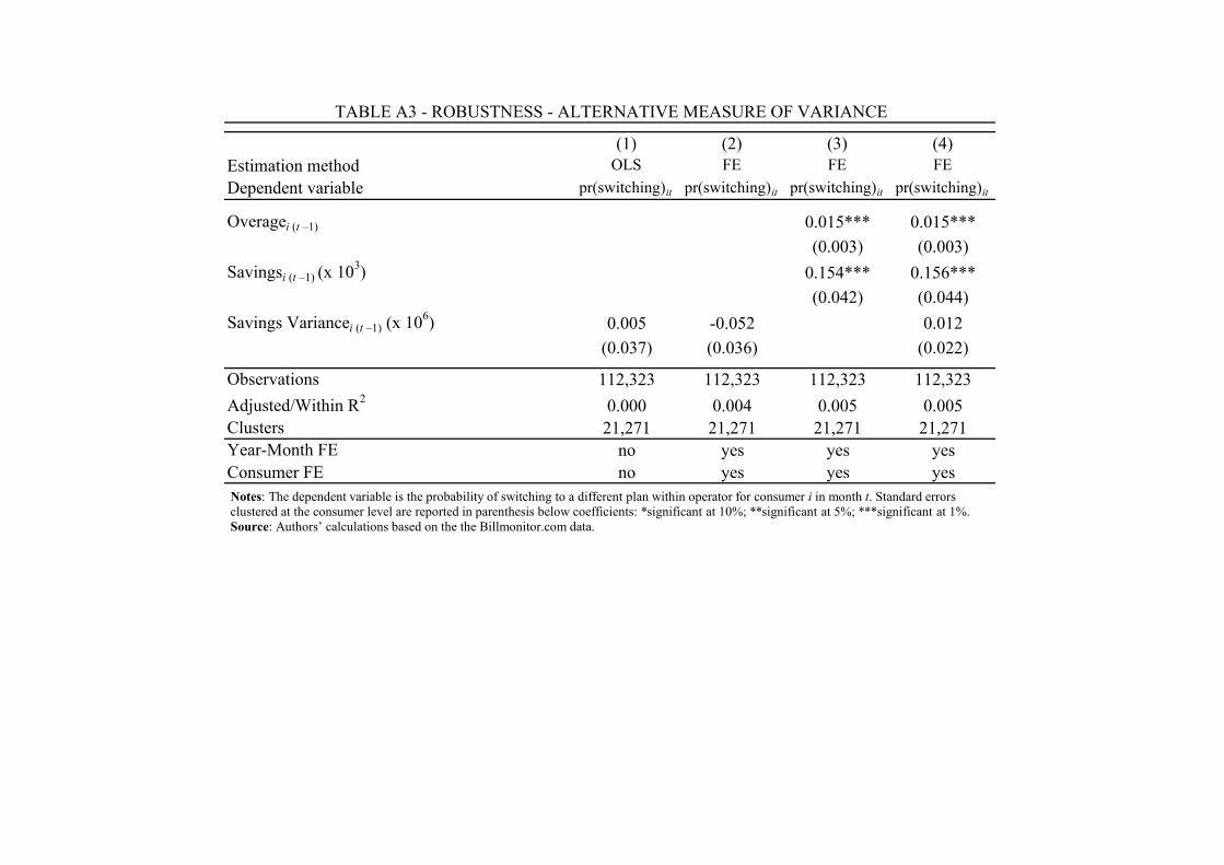
(1) (2) (3) (4)

Estimation method OLS FE FE FE

Dependent variable pr(switching)it pr(switching)it pr(switching)it pr(switching)it

Overagei (t –1) 0.015*** 0.015***

(0.003) (0.003)

Savingsi (t –1) (x 103) 0.154*** 0.156***

(0.042) (0.044)

Savings Variancei (t –1) (x 106) 0.005 -0.052 0.012

(0.037) (0.036) (0.022)

Observations 112,323 112,323 112,323 112,323

Adjusted/Within R2

0.000 0.004 0.005 0.005

Clusters 21,271 21,271 21,271 21,271

Year-Month FE no yes yes yes

Consumer FE no yes yes yes

TABLE A3 - ROBUSTNESS - ALTERNATIVE MEASURE OF VARIANCE

Notes: The dependent variable is the probability of switching to a different plan within operator for consumer i in month t. Standard errors

clustered at the consumer level are reported in parenthesis below coefficients: *significant at 10%; **significant at 5%; ***significant at 1%.

Source: Authors’ calculations based on the the Billmonitor.com data.

CENTRE FOR ECONOMIC PERFORMANCE Recent Discussion Papers

1372 Shaun Larcom Ferdinand Rauch Tim Willems

The Benefits of Forced Experimentation: Striking Evidence from the London Underground Network

1371 Natalia Ramondo Veronica Rappoport Kim J. Ruhl

Intrafirm Trade and Vertical Fragmentation in U.S. Multinational Corporations

1370 Andrew Eyles Stephen Machin Olmo Silva

Academies 2: The New Batch

1369 Yonas Alem Jonathan Colmer

Consumption Smoothing and the Welfare Cost of Uncertainty

1368 Andrew Eyles Stephen Machin

The Introduction of Academy Schools to England’s Education

1367 Jeremiah Dittmar Skipper Seabold

Media, Markets and Institutional Change: Evidence from the Protestant Reformation

1366 Matthew D. Adler Paul Dolan Georgios Kavetsos

Would you Choose to be Happy? Tradeoffs Between Happiness and the Other Dimensions of Life in a Large Population Survey

1365 Jeremiah Dittmar New Media, Competition, and Growth: European Cities After Gutenberg

1364 Jenifer Ruiz-Valenzuela Job Loss at Home: Children’s School Performance during the Great Depression in Spain

1363 Alex Bryson John Forth Lucy Stokes

Does Worker Wellbeing Affect Workplace Performance?

1362 Joan Costa-Font Frank Cowell

European Identity and Redistributive Preferences

1361 Jonas Kolsrud Camille Landais Peter Nilsson Johannes Spinnewijn

The Optimal Timing of UI Benefits: Theory and Evidence from Sweden

1360 Joan Costa Font Martin Karlsson Henning Øien

Informal Care and the Great Recession

1359 Benjamin Faber Rosa Sanchis-Guarner Felix Weinhardt

ICT and Education: Evidence from Student Home Addresses

1358 Esther Ann Bøler Beata Javorcik Karen Helene Ulltveit-Moe

Globalisation: A Woman's Best Friend? Exporters and the Gender Wage Gap

1357 Michael Amior Alan Manning

The Persistence of Local Joblessness

1356 Sarah Flèche Richard Layard

Do More of Those in Misery Suffer From Poverty, Unemployment or Mental Illness?

1355 Mirko Draca Theodore Koutmeridis Stephen Machin

The Changing Returns to Crime: Do Criminals Respond to Prices?

1354 Jae Song David J. Price Fatih Guvenen Nicholas Bloom

Firming Up Inequality

1353 Gianmarco I. P. Ottaviano Giovanni Peri Greg C. Wright

Immigration, Trade and Productivity in Services: Evidence from UK Firms

1352 Joanne Blanden Emelia Del Bono Sandra McNally Brigitta Rabe

Universal Pre-School Education: The Case of Public Funding With Private Provision

The Centre for Economic Performance Publications Unit Tel 020 7955 7673 Fax 020 7404 0612

Email info@cep.lse.ac.uk Web site http://cep.lse.ac.uk