CEP Discussion Paper No 700

July 2005

The Gender Gap in Early-Career Wage Growth

Alan Manning and Joanna Swaffield

Abstract In the UK the gender pay gap on entry to the labour market is approximately zero but after ten years after labour market entry, there is a gender wage gap of almost 25 log points. This paper explores the reason for this gender gap in early-career wage growth, considering three main hypotheses - human capital, job-shopping and ‘psychological’ theories. Human capital factors can explain about 12 log points, job-shopping about 1.5 log points and the psychological theories about half a log point. But a substantial unexplained gap remains: women who have continuous full-time employment, have had no children and express no desire to have them earn about 12 log points less than equivalent men after 10 years in the labour market. Keywords: Gender Pay Gap, Wage Growth JEL Classifications: J24, J31, J7 Data: BHPS, BCS, NES, LFS This paper was produced as part of the Centre’s Labour Markets Programme. The Centre for Economic Performance is financed by the Economic and Social Research Council. Acknowledgements This paper was presented at Warwick and CEP seminars. Alan Manning is a Programme Director at the Centre for Economic Performance and Professor of Economics, London School of Economics. Email: Joanna Swaffield is a Lecturer in the Department of Economics, The University of York. Email: jks4@york.ac.uk Published by Centre for Economic Performance London School of Economics and Political Science Houghton Street London WC2A 2AE All rights reserved. No part of this publication may be reproduced, stored in a retrieval system or transmitted in any form or by any means without the prior permission in writing of the publisher nor be issued to the public or circulated in any form other than that in which it is published. Requests for permission to reproduce any article or part of the Working Paper should be sent to the editor at the above address. © A. Manning and J. Swaffield, submitted 2005 ISBN 0 7530 1880 2

1

Introduction

This paper is about the gender pay gap in the UK. Given the enormous literature on

the gender pay gap (see Altonji and Blank, 1999, for a relatively recent survey) one

might wonder about the justification for yet another paper on the subject. The answer

is that this paper focuses on the gender gap in wage growth in the early years after

labour market entry and argues that an understanding of this is necessary as it is the

primary cause of the overall gender pay gap. The reason why this is particularly

important in the UK can be explained very simply.

Figure 1 presents the data the earnings-experience profile in the UK for men

and women together with the gender pay gap from one of the main data sets used in

this paper, the British Household Panel Survey (BHPS). Average log wages are

normalized to be zero for men with zero years of labour market experience. One can

see that the earnings of men and women are very similar on entry to the labour market

but 10 years later a sizeable gender gap in earnings has emerged, a gap that reaches its

maximum about 20 years after labour market entry before falling slightly in later

years1. Of course, cross-section profiles like the ones presented in Figure 1 confound

true life-cycle effects and cohort effects. But, while cohort effects can probably

explain some of the cross-section profile, there is good reason to think that they are

not the most important reason for the widening of the gender pay gap after labour

market entry. To see this Figure 2 presents the gender earnings gap at different ages

for different birth cohorts in the New Earnings Survey (NES)2. The NES contains no

information on education (so we cannot compute experience) and Figure 2 simply

presents age profiles. What one can see is that the gender pay gap is lower at all ages

for younger cohorts but that the contribution of cohort is small relative to the life- 1 This convergence in later years is less apparent in the BHPS then in other British data sets like the Labour Force Survey. 2 The BHPS is too short a panel to follow cohorts through time.

2

cycle effects. For example, Figure 2 suggests that the gender pay gap that can be

expected at age 40 for those born around 1970 is likely to be smaller than for those

born around 1960 but extrapolation of the profiles in Figure 2 would suggest that a

very sizeable gender wage gap will still exist. And for women born after 1970 there

is some evidence that the progress of women has stalled as the profiles of the gender

pay gap are very similar for those born around 1970 and those born in the late 1970s –

if this is true then there will be a gender pay gap for these women of 20 log points in

their early 30s3. So, young women entering the labour market today can still expect to

earn much less than young men after 10 years in the labour market and this gender

difference in early-career wage growth needs explaining.

Most papers on the gender pay gap focus on the level of pay and not the

growth in pay. But as the level of pay at any level experience is simply the initial pay

on labour market entry plus cumulated wage growth any theory of the pay level must

be, if only implicitly, also a theory of wage growth (and vice versa). So, theories to

explain the level of pay should also be able to explain differences in wage growth.

This paper focuses on three theories of wage growth – the human capital hypothesis,

job-shopping and ‘psychological’ theories and asks how well they can do in

explaining the gender gap in early-career wage growth.

The most common approach to explaining the gender pay gap is based on the

human capital model developed by Becker (1993) and Mincer (1974) and applied to

the gender pay gap in many papers (e.g. see Mincer and Polachek, 1974, Mincer and

Ofek, 1982, Light and Ureta, 1995 inter alia). This approach seeks to explain the

gender pay gap by gender differences in human capital accumulation of which there

are several dimensions. First, there are gender differences in accumulated work 3 The flattening in the gender pay gap that one sees in the early 20s in Figure 2 is the result of the entry at that age into the labour market of college graduates for whom, on labour market entry, the gender pay gap is small.

3

experience (which is assumed to be correlated with levels of human capital) because

women are more likely to have intermittent labour market participation and are more

likely to work part-time. Secondly, the anticipation of future intermittence may affect

current investments in human capital. The affected investments might be after labour

market entry (see Ben-Porath, 1967, for a classic theoretical model of this) or prior to

labour market entry where it may take the form of gender differences in the quantity

or (more plausible these days for a country like the UK) type of education. Thirdly,

Becker (1985) has argued that the greater domestic commitments of women

(especially married women with dependent children) means they put less energy into

work and that translates into lower hourly wages.

The estimates presented below find that the human capital hypothesis can

explain some of the gender gap in early-career wage growth but most of the gender

pay gap that emerges by 10 years after labour market entry cannot be explained in this

way. The reason for this conclusion can be explained very simply. First, differences

in actual labour market experience between young British men and women after 10

years in the labour market are simply not large enough to explain more than 6.5 of the

25 log-point gender pay gap at that point in the life-cycle. Secondly, gender

differences in job-related training do explain a part of the differential (primarily

because young men are still much more likely than young women to go into

apprenticeships) but, again, the estimated contribution is no more than 4.5 log points.

And, thirdly, gender differences in the quantity of education are very small (and, in

any case, Mincer’s (1974) famous observation that the experience profiles are similar

for different levels of education would suggest that any difference in the quantity of

education should show up in a gender pay gap on labour market entry and not a

gender gap in wage growth), and, while gender differences in the types of education

4

and associated occupational choices are still large, we do not find that occupational

differences contribute much to the gender gap in early-career wage growth. The

bottom line is that the human capital explanations can explain perhaps half of the 25

log point gender pay gap observed 10 years after labour market entry.

The paper then also investigates the job-shopping hypothesis that an important

part of early career wage growth is associated with moving from worse to better-

paying jobs (e.g. Topel and Ward, 1992 who study only US men find that something

like one-third of wage growth in the first 10 years after labour market entry can be put

down to job mobility). Manning (2003a, ch7) has documented how women are more

constrained in their opportunities to change jobs than men and are less concerned with

money when they do. So we might expect to see women making fewer ‘good’ job

changes, more ‘bad’ job changes and a lower return to job changes when they do. We

investigate this hypothesis below, and find that it can explain only 1.5 log points of

the gender pay gap after 10 years in the labour market. This is not because job

mobility is unimportant but because gender differences in job mobility among young

workers are quite small.

The paper then considers a more recent but less well-known theory of the

gender pay gap – that has its roots in psychological differences in the behaviour of

men and women that they bring with them to the labour market. In their book,

‘Women Don’t Ask: Negotiation and the Gender Divide’, Babcock and Laschever

(2003) argue that a powerful cause of women’s disadvantage is that they tend to have

a lower opinion of themselves than men so do not ask their bosses for what they want

and passively accept wage offers rather than bargain for better conditions. We use

data on psychological attributes of men and women before labour market entry to test

this hypothesis. We find that there are returns to ‘personality’ (as has been found by

5

others – see Goldsmith et al, 1997, Feinstein, 2000, Bowles et al, 2001) but the gender

differences and the returns are not large enough to explain more than roughly half a

log point of the gender pay gap that emerges after 10 years in the labour market.

The plan of the paper is as follows. The next section describes the data used in

the paper. The second section then presents ‘reduced-form’ estimates of wage growth

equations that confirm the presence of a gender gap in early-career wage growth as

suggested by Figure 1. The third section then investigates the extent to which this can

be explained by differences in human capital considering the contribution of breaks in

employment, of job-related training, of the types of education and of occupational

choice. The fourth section then considers the contribution of job mobility, both good

and bad, to wage growth. The fifth section then investigates the importance of

‘personality’ for explaining the gender pay gap. The bottom line is that a considerable

part of the gender pay gap after 10 years in the labour market remains unexplained: a

woman who has done nothing but work full-time ever since leaving education, has

had no children and expresses no desire to have them in the future earns, on average,

at least 10 percentage points less than an equivalent man. The conclusion makes

some suggestions about possible directions for further research.

1. The Data

The main data used in the first part of this paper comes from the first 12 waves

of the British Household Panel Study (BHPS) that cover the period 1991-2002

inclusive though the Labour Force Survey (LFS) the New Earnings Survey (NES) are

sometimes used for supplementary evidence and consistency checks. The BHPS

started in 1991 with some 5500 households and 10,300 individuals drawn from 250

different areas of Great Britain. It has had a number of booster samples:

6

approximately 1000 households in 1997 that are part of the European Community

Household Panel Survey (that include Northern Ireland and over-sample low-income

households), approximately 3000 Scottish and Welsh households that were added in

1999. It follows all individuals in sample households and those who end up in

households with them as long as they remain in a household with an original sample

member (in many ways, it can be thought of as the British PSID).

From the BHPS the sample is constructed in the following way. First, the

sample is restricted attention to those with no more than 10 years of potential labour

market experience as our focus is on what happens to the gender pay gap in the years

after labor market entry. Secondly, only those individuals for whom there is an

uninterrupted set of interviews are included. Thirdly, anyone who has a period in

employment when we cannot identify whether they are working for the same

employer as at the previous interview is excluded. Finally, because of the difficulty in

measuring earnings for the self-employed anyone who reported being self-employed

at any interview date is excluded: as few individuals move between employment and

self-employment (about 1.5% of employees become self-employed in any year) this is

a relatively minor restriction. In total about 5% of observations are excluded because

of data problems and the final sample used for analysis is approximately 10500

observations on wage growth for about 3559 individuals.

Wages are measured as an hourly rate, obtained by dividing usual weekly

earnings by usual weekly hours. Those with hourly earnings below £1 or above £100

are excluded. As we do not want the measure of earnings growth on-the-job to

include aggregate wage growth it is important to deflate wages: as Altonji and

Williams (1998) point out, estimates of the return to job tenure can be sensitive to the

7

way in which this is done4. We experimented with the use of an external earnings

index but average earnings growth in the BHPS deviates from this aggregate measure.

As a result we estimated a simple earnings function of the log of hourly wages on a

quartic in experience, regional, race and gender dummies and a set of wave dummies

and then deducted the wave dummies to generate our adjusted wage series.

As we are interested in how wages evolve, we need a measure of wage

growth. In most studies of wage growth, the dependent variable is defined as the

growth in wages between two fixed points in time, with this measure being undefined

for those who are not in employment at either of the two points. This approach has

the disadvantage that it under-samples those individuals who have intermittent

employment, a potentially serious problem when analyzing the gender pay gap. For

example, suppose we measure wages annually but some individuals have a year or

more in which they are not in employment. If one only measures wage growth from

one year to the next, one will drop two observations for such individuals because there

will be two years in which annual wage growth is not defined. To deal with this

problem, we define wage growth in the following way. For any year in which an

individual is in employment, define the wage growth as the difference in log wages

between the next year they are in employment and the log wage this year.

Consequently there may be gaps between the two wage observations of any number of

years. It is important to control for this ‘gap’ in what follows and we describe later

how we do this. There remains a potential problem in that the gap between wage

observations is censored at the top end by the latest year of observation being 2002

4 This is less important in the current context where we are primarily interested in the gender gap in wage growth than in the literature on the returns to job tenure as incorrect detrending probably has a very similar effect on both men and women.

8

but this seems to be a small problem5 because long gaps between wage observations

are relatively rare. The first two columns of Table 1 presents the distribution of gaps

between the wage observations in our data set for men and women. One observes, as

one would expect, that women are more likely than men to have intermittent

employment. But, what is also striking is the relatively short length of gaps between

periods of employment (see also Myck and Paull. 2001, for an analysis of gender

differences in accumulated experience). Only 2% of the observations on female wage

growth have a gap in employment of more than 2 years. Because the BHPS is a

relatively short panel, there are many censored observations so, to get some idea of

the uncensored distribution of the gap the third and fourth columns of Table 1 report

the distribution of the gap among those in waves 1-6. There are now more young

women with longer gaps in employment though it remains remarkable how rare are

long breaks in employment. However this data is still censored: some women may

never return to paid employment but some might have very long spells that are not

observed in the BHPS. To get some idea of this, the final two columns of Table 1

presents, for comparison, data on gaps between spells of employment from the LFS.

In the LFS those not currently in employment are asked when they last worked and

we can use this information to work out the gap between employment spells for those

who are employed in the subsequent quarter6. Again, one sees that women are more

likely to have gaps in employment than men but the average size of gaps and the

gender differences are not large – the BHPS suggests an average gap for women that

is 0.3 years above that for men and the LFS suggests a somewhat smaller gap of 0.25

years. And the very long gaps that contribute quite a lot to this overall gender

5 We did experiment with restricting the sample to those in the early waves when censoring is less problematic: this made no difference to the conclusions. 6 Note that in a steady-state it should not matter whether one looks forward as in the BHPS or backwards as in the LFS.

9

difference are very rare among the young workers that are the focus of this paper. For

example, the work history data of the 1970 British Cohort Study suggests that, among

those in employment at age 30, 23% of men have had a period of non-employment

between two periods of employment with an average of 0.3 gaps compared to 27% of

women with an average of 0.35 gaps.

One other peculiarity of the BHPS that is worth mentioning is that its basic

measure of job tenure is tenure in a particular job with a particular employer so that

within-firm changes of job reset the tenure clock to zero. This is not the way that the

job tenure variable is usually defined where it refers to job tenure with the same

employer. However, the BHPS definition is retained here as job moves within

employers (e.g. promotions) are as interesting and important as those between

employers in understanding the emergence of the gender pay gap7. The data is

summarized in the Appendix in Table A1.

2. Reduced Form Estimates

While the evidence presented in Figures 1 and 2 is strongly suggestive of a

gender gap in wage growth in the years immediately after labour market entry, it is

important to verify this using direct data on wage growth. Hence, this section

presents some ‘reduced-form’ wage growth regressions to get some idea of what the

data looks like and to confirm the existence of this gender gap in early-career wage

growth.

Accordingly, we estimate the following ‘reduced-form’ model for the wage

growth between t and (t+g) of individual i where g is the gap between wage

observations: 7 Furthermore, attempting to construct more traditional measures of job tenure results in a large fall in the number of useable observations because the work history information needed to construct it is only available for a fraction of the sample.

10

20 1 2 ( )it it it it it itw e e eβ β β ε φ ε∆ = + + + = + (1)

where e is years since leaving full-time education i.e. potential experience. This

model is estimated separately for men and women. The quadratic specification seems

adequate to capture the variation in wage growth among the young workers in our

sample but one should be wary of extrapolating into other parts of the life-cycle

(Murphy and Welch, 1990, suggest a quartic for the level implying a cubic for the

change if workers of all ages are in the sample).

In specifying this equation we need to be careful about how we deal with

individuals for whom the gap over which wage growth is measured is more than a

year. To see why this matters suppose that the observed wage growth for all

individuals (whatever the gap) was 5% but that men are always in employment (so

g=1) but women are only in employment every two years (so g=2). After 2 years

earnings for men would have grown by approximately 10% whereas those for women

would have only grown by 5%. The gender pay gap would be widening but

estimation of (1) that did not take account of differences in the gap would miss this.

The simplest way of getting a gap-adjusted measure of wage growth would be

to simply divide the observed wage growth by the gap between wage observations to

get an estimate of annualized wage growth. However the validity of this procedure is

based on the implicit assumption that wage growth does not vary with experience,

something we know to be untrue. So, a slightly more sophisticated approach is taken

here to adjust for the gap between wage observations. If (1) is the wage growth for

those for whom g=1, then for someone with g=2 to return to employment at the same

level of wages they must have expected wage growth between the two observations

of:

( ) ( ) ( 1)it it itE w e eφ φ∆ = + + (2)

11

the right-hand side of which is simply two one-period sets of wage growth. One can

readily extend this formula to any value of g in which case it will be given by:

( ) 1

0( )g

it itjE w e jφ−

=∆ = +∑ (3)

Using the specific functional form in (1), this can be written as:

( ) 1 1 20 1 20 0

( ) ( )g git it itj j

E w g e j e jβ β β− −

= =∆ = + + + +∑ ∑ (4)

Thus one can readily estimate wage growth on a consistent basis for individuals with

different gaps by computing the ‘adjusted’ levels of experience in (4) and using these

as regressors in a wage growth equation. Note that there is no constant in this

regression - the constant in (1) gets multiplied by g. If wage growth does not vary

with experience this approach is equivalent to the simple-minded approach of just

dividing wage growth by the interval between wage observations as the gap would be

the only remaining regressor and the coefficient on it can be interpreted as annual

wage growth.

Table 2 reports estimates of the reduced-form wage growth equations. The first two

columns of Table 2 report estimates of (4) for men and women separately. We report

the estimates of earnings growth at 0, 5 and 10 years of experience together with their

standard errors. Taking the coefficients for men, the estimates suggest that a man can

expect 14.5% annual wage growth on entry into the labour market, falling to 6.8%

after 5 years and 1.3% after 10 years. For women (the second column) earnings

growth on entry is lower than for men (at 12.0% per annum) and still lower after 10

years though the gap in wage growth narrows8. These estimates are consistent with

the finding that the gender pay gap begins to widen soon after labour market entry, as

8 One might wonder whether these gender differences are significantly different from each other. At each individual level of experience the answer is often ‘no’ but one can easily reject the joint hypothesis that the returns to experience for men and women are equal in the first 10 years.

12

suggested in Figure 19. The bottom two rows of Table 2 report the gender pay gap

implied by these differences in estimated wage growth 5 and 10 years after labour

market entry. These are derived by cumulating the estimates of the gender difference

in wage growth from the estimation of (4) assuming that there are no breaks in

employment and (as is a good approximation) that gender differences in wages on

labour market entry are zero. The estimates in columns 1 and 2 of Table 2 imply a

gender pay gap of 14.4 log points after 5 years and 24.8 log points after 10 years.

These estimates are not far out of line with those derived from estimates of wage

levels.

To check that these estimates are not sensitive to the treatment of those with gaps

of more than 1 year between wage observations, columns 3 and 4 of Table 2 present

the ‘reduced-form’ wage growth equations restricting the sample to those for whom

the gap between wage observations is only one year. One finds the same pattern of

gender differences in wage growth. The implied gender pay gap after 10 years is

lower for this sample at 22.2 log points suggesting that part of the overall gap can be

explained by women having more intermittence but the contribution is not that large,

suggesting that there are not large gender gaps in labour market attachment among

young workers.

One might also wonder whether the inclusion of other controls on individual

characteristics alter these conclusions. The bottom line is that they do not have a big

impact10. One way to see the irrelevance of personal characteristics is to estimate

9 Note that, averaging across men and women of all experience levels, there is no significant difference in wage growth - as found by Manning and Robinson (2004). However, that paper makes the (embarrassing) mistake of inferring from this fact that gender differences in wage growth cannot explain the gender pay gap. This is wrong because a male advantage in wage growth in early life off-set by a female advantage in later life does not imply a zero gender pay gap. 10 One proviso to this is that there is some evidence that in the reduced form, the earnings growth is lower in the early years for the best-educated. But, this can be explained by the larger amount of on-the-job training received in the early years by the less-educated and this is a variable for which we do control later in the paper.

13

wage growth equations including individual fixed effects. This is done in the final

two columns of Table 2: the coefficients hardly change and the fixed effects are

jointly insignificant from zero. We should not be surprised by this finding: if there

were very significant permanent differences in wage growth across individuals one

would expect to see the variance of earnings in a cohort rising explosively over the

life-cycle which it does not11. Of course, this insignificance of fixed effects in a

wage-growth equation does not mean that individual fixed effects would not be very

significant in a wage levels equation – rather, it is a validation of Mincer’s conclusion

that earnings profiles are parallel to each other (once one controls for gender).

So, our basic data do contain the feature that there is a noticeable gender gap

in wage growth from the start of labour market careers. Although this gender gap in

wage growth eventually reverses there is a very large gender pay gap by the time it

does and women never make up the ground lost in the first 10 years after labour

market entry. One might be concerned that this conclusion applies only to the BHPS

or is an artifact of the quadratic specification used. So, as a useful double-check,

Figure 3 presents data from the NES that has a large enough sample size to get precise

estimates of wage growth for men and women at each age. This shows the same

pattern as the BHPS. It is this gender gap in early-career wage growth that this paper

seeks to explain.

3. Gender Differences in Human Capital Accumulation

Human capital theories seek to explain the gender pay gap by gender differences in

human capital accumulation. There is no doubt that human capital theory is of use in

explaining at least some part of the gender pay gap – some researchers (e.g. O’Neill,

11 See Mincer (1974) and, more recently, by Heckman Lochner and Todd (2002) for a discussion of the variance profile.

14

2003, and Polachek, 2004) claim that it can explain virtually all of the US gender pay

gap while others (e.g. Altonji and Blank, 1999, Blau and Kahn, 2004), find that there

remains a sizeable unexplained component to the gender pay gap. There are several

varieties of human capital explanations for the gender pay gap all of which have their

root in “the lesser amount of time and energy that women can commit to labour-

market careers as a result of the division of labour within the family” (O’Neill, 2003,

p309). First, after labour market entry, the weaker labour market attachment of

women means they tend to accumulate less labour market experience than men and,

given that such experience is valuable, part of the difference in earnings can be

explained as the result of this difference in actual labour market experience. Studies

(e.g. see Mincer and Polachek, 1974, or Light and Ureta, 1995) sometimes find that

the returns to actual experience is very similar for men and women though typically

other measures of labour market history are also important in explaining the gender

pay gap and a sizeable part of the gender pay gap remains unexplained even after

controlling for differences in actual labour market experience12.

Secondly, there may be differences in human capital investments after labour

market entry in anticipation of future labour market attachment. So, we might see

men doing more job-related training than women because they expect to spend longer

in the labour market in later years. Thirdly, a similar argument might apply to human

capital investments in education prior to labour market entry – men might make more

investments than women in human capital that has a labour market pay-off. We

consider these three different human capital hypotheses in turn.

12 And one should also note that actual labour market experience is endogenous so that part of the correlation of wages with actual experience may not be causal.

15

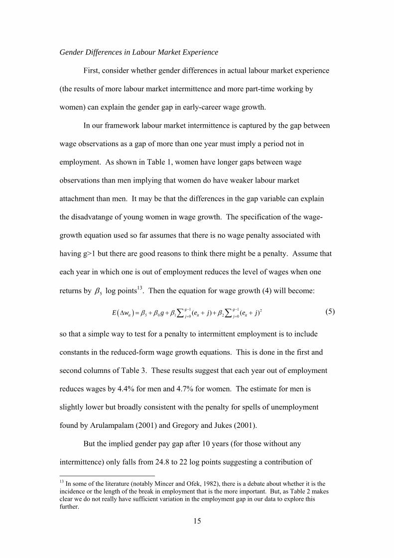
Gender Differences in Labour Market Experience

First, consider whether gender differences in actual labour market experience

(the results of more labour market intermittence and more part-time working by

women) can explain the gender gap in early-career wage growth.

In our framework labour market intermittence is captured by the gap between

wage observations as a gap of more than one year must imply a period not in

employment. As shown in Table 1, women have longer gaps between wage

observations than men implying that women do have weaker labour market

attachment than men. It may be that the differences in the gap variable can explain

the disadvatange of young women in wage growth. The specification of the wage-

growth equation used so far assumes that there is no wage penalty associated with

having g>1 but there are good reasons to think there might be a penalty. Assume that

each year in which one is out of employment reduces the level of wages when one

returns by 5β log points13. Then the equation for wage growth (4) will become:

( ) 1 1 25 0 1 20 0

( ) ( )g git it itj j

E w g e j e jβ β β β− −

= =∆ = + + + + +∑ ∑ (5)

so that a simple way to test for a penalty to intermittent employment is to include

constants in the reduced-form wage growth equations. This is done in the first and

second columns of Table 3. These results suggest that each year out of employment

reduces wages by 4.4% for men and 4.7% for women. The estimate for men is

slightly lower but broadly consistent with the penalty for spells of unemployment

found by Arulampalam (2001) and Gregory and Jukes (2001).

But the implied gender pay gap after 10 years (for those without any

intermittence) only falls from 24.8 to 22 log points suggesting a contribution of

13 In some of the literature (notably Mincer and Ofek, 1982), there is a debate about whether it is the incidence or the length of the break in employment that is the more important. But, as Table 2 makes clear we do not really have sufficient variation in the employment gap in our data to explore this further.

16

intermittence of 2.8 log points (this is similar to the estimate from columns 3 and 4 of

Table 2).

Women accumulate less work experience than men, not just because they have

more intermittence but also because they are more likely to work part-time. For

example, in our sample, 3.6% of the men are working part-time (defined as less than

30 hours a week) and 19.2% of the women. The third and fourth columns of Table 3

include a dummy variable for whether the individual is currently working part-time.

The few men who are working part-time have a very large penalty of 19.3 log pints

while the part-time women have a pay penalty of 6.0%. The implied gender gap after

10 years for those who work continuously full-time now falls to 18.3% suggesting a

contribution of the gender difference in part-time working of 3.7%. This is probably

an over-estimate as hourly earnings are obtained by dividing weekly earnings by

reported hours leading to a division bias problem that overstates the initital wages of

those in part-time employment.

The estimates so far suggest that differences in actual work experience when

young can explain at most 30% of the gender gap in early-career wage growth. The

explanation for this is simple: the gender gap in wage growth is largest when the

gender gap in accumulated actual labour market experience is rather small. To further

illustrate this Figure 4 presents data from the 1970 British Cohort Study, a

longitudinal of all children born in Britain in one week in 1970 and which collects

monthly information on labour market status. Figure 4 shows the gender differences

in actual experience (measured as months in work) over the first 10 years after labour

market entry. 10 years after labour market entry the men have accumulated about 12

months more work experience than the women. The gap in full-time experience is

larger at 20 months. However, for the purpose of understanding the gender pay gap

17

for those in work (as is the focus of this paper) these differences are misleading as the

pay differences relate to those in work and the gender differences in actual experience

are much smaller for those in work. These differences are also plotted on Figure 4:

after 10 years male workers have about 3 months more work experience than women

and about 12 months more full-time experience. These differences are simply not

large enough to explain the magnitude of the gender pay gap after 10 years: for

example, if one thinks of the male profile as being the ‘true’ one and women are one

year behind men after 10 years this can only account for wage differentials of the

order of 2 log points. The contribution is a bit larger if one recognizes that the

earnings profile is concave so it is not just the mean but also the variance that is of

importance and women have slightly higher variance than men. After 10 years the

gender difference in the variance of full-time work experience among workers is

about 1 year which adds at most an extra one log point to the predicted gender

difference These back-of-the-envelope calculations are smaller than the regression

estimates of Table 3 though, as we have already noted, the contribution of part-time

working is probably over-estimated.

The discussion so far has focused on the accumulation of general human

capital but gender differences in the accumulation of specific human capital might

also be important. Job-specific human capital is often assumed to be measured by job

tenure (see Mincer and Jovanovic, 1981, for this theoretical argument and Jones and

Makepeace, 1996, for a British study in which this variable is important for explaining

a gender gap). The fifth and sixth columns of Table 3 include job tenure in the

current job as an extra control in the wage-growth equations. We find that higher job

tenure is associated with significantly lower wage growth. But, this does little to

narrow the gender gap in wage growth on labour market entry and has no impact on

18

the implied gender pay gap after 10 years.

Gender Differences in On-the-Job Training

Of course, it may be differences in expected future labour market attachment that

affect current human capital accumulation either before or after labour market entry.

Let us start with the training after labour market entry. In the BHPS respondents are

asked about the total amount of job-related training they have done over the previous

year. We simply include a measure of the total years of training received as a control

variable in our wage growth regression. We might expect that current job-related

training depresses current wages but raises future wages and wage growth. However,

the strongest empirical effect of on-the-job training seems to come not from the

measure of the training received between the two wage observations but from the

measure of training received over the year prior to the initial wage observation. So,

measures of training in both years are included in the wage growth regressions: the

results are presented in columns 7 and 8 of Table 3. The return to a year of job-

related training for men is higher (at approximately 8-10%) than for women

(approximately 3% for training received in the past year and zero for training between

wage observations).

The difference in the return to training is compounded by the fact that young

men receive more on-the-job training than young women – for example among

workers with less than 5 years of potential experience, the men receive on average

0.039 years of training per year and the women 0.032. This seems to be the result of

the fact that men (especially those with little education) are much more likely than

women to be in apprenticeships (which have a very large training component).

Among men who leave school at 16 but are aged 20 or under 25% are in

19

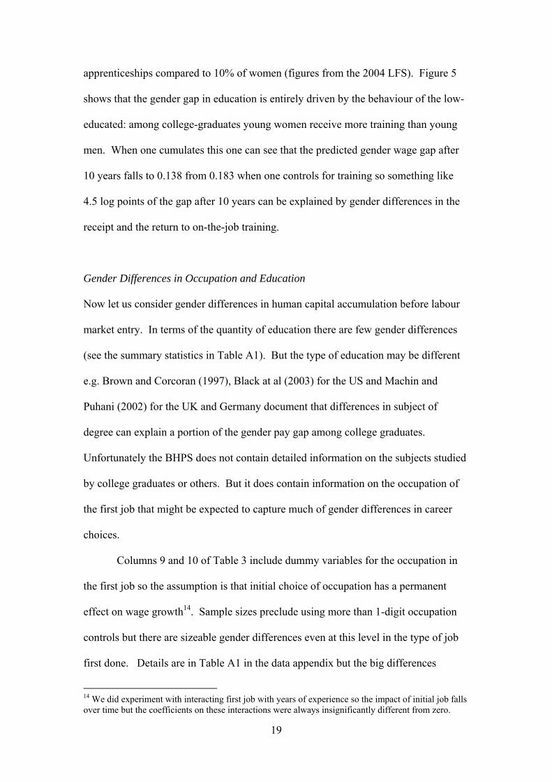
apprenticeships compared to 10% of women (figures from the 2004 LFS). Figure 5

shows that the gender gap in education is entirely driven by the behaviour of the low-

educated: among college-graduates young women receive more training than young

men. When one cumulates this one can see that the predicted gender wage gap after

10 years falls to 0.138 from 0.183 when one controls for training so something like

4.5 log points of the gap after 10 years can be explained by gender differences in the

receipt and the return to on-the-job training.

Gender Differences in Occupation and Education

Now let us consider gender differences in human capital accumulation before labour

market entry. In terms of the quantity of education there are few gender differences

(see the summary statistics in Table A1). But the type of education may be different

e.g. Brown and Corcoran (1997), Black at al (2003) for the US and Machin and

Puhani (2002) for the UK and Germany document that differences in subject of

degree can explain a portion of the gender pay gap among college graduates.

Unfortunately the BHPS does not contain detailed information on the subjects studied

by college graduates or others. But it does contain information on the occupation of

the first job that might be expected to capture much of gender differences in career

choices.

Columns 9 and 10 of Table 3 include dummy variables for the occupation in

the first job so the assumption is that initial choice of occupation has a permanent

effect on wage growth14. Sample sizes preclude using more than 1-digit occupation

controls but there are sizeable gender differences even at this level in the type of job

first done. Details are in Table A1 in the data appendix but the big differences

14 We did experiment with interacting first job with years of experience so the impact of initial job falls over time but the coefficients on these interactions were always insignificantly different from zero.

20

among young workers (with less than 10 years of potential experience) are that 38%

of women first enter clerical and secretarial occupations compared to 16% of men,

20% of women enter personal and protective service occupations compared to 8% of

men, 2% of women enter craft occupations compared to 23% of men and 7% of

women enter elementary occupations compared to 15% of men.

In producing the summary statistics on wage growth at different levels of

experience and the gender gap we assume a distribution of first jobs equal to the

average across men and women with less than 10 years of experience – evaluating at

male or female characteristics makes no difference. For both men and women the

coefficients on initial occupation are jointly not significantly different from zero

though the rejection is marginal for men (the rather curious mix of managerial,

professional, clerical and elementary occupations seem to have higher wage growth

than the others). But, when it comes to explaining gender differences in wage growth,

initial occupation has little explanatory power with the predicted gender pay gap after

10 years falling from 0.138 to 0.124 after controlling for initial occupation15.

However this evidence has only used 1-digit controls for initial occupation and

one might be concerned that more marked differences would emerge if a finer

measure of occupation was used. That is not possible because of small sample sizes

in the BHPS but we can get some idea of whether this is likely using the much larger

sample sizes available in the NES where we can use 3-digit occupation of which there

are approximately 370. Once one goes to this level of disaggregation there is a

problem that some occupations are so overwhelmingly dominated by one gender that

one has very few observations on the other. To deal with this problem of matching 15 One might be concerned that the sample sizes in columns 9 and 10 are considerably smaller than in columns 7 and 8 because initial job is missing for many observations. But, estimating the model of columns 7 and 8 using the restricted sample of columns 9 and 10 leads to a predicted wage gap after 10 years of 0.13 so the contribution of occupation is probably smaller than it appears from a simple inspection of Table 3.

21

men and women at the 3-digit occupation level the sample is restricted to occupations

that have at least 2% of the minority gender. This excludes from the sample 17.5% of

men in 74 occupations (broadly, production managers in manufacturing and

construction, senior police and fire officers, drivers of trains, boats, and planes, almost

all of construction, almost anything that involves metal-working, and refuse

collection). 9.6% of women are excluded in 9 occupations (broadly, midwives,

secretaries, dental nurses, childcare workers and beauticians).

We take two approaches to controlling for occupation. In the first we simply

include a dummy variable for each occupation in the gender-specific wage growth

equations effectively assuming that occupation only affects the level and not the life-

cycle profile of wage growth. The results are summarized in Panel A of Figure 6.

The line marked ‘whole sample’ reproduces the raw gender gap in wage growth

already shown in Figure 4. The line ‘matched sample’ reports the raw gap in wage

growth for those in occupations that are not excluded from the analysis – one notices

that the gender gap in wage growth is now much smaller for those aged 16-22. The

most likely explanation for this finding is that many of the men who are excluded

from the matched sample are in construction and/or metal-working trades and the

young men in particular are doing apprenticeships that is associated with fast wage

growth. This is consistent with our earlier finding of gender differences in training

receipt among this group.

The remaining two lines in Figure 6A show the impact of adjusting the

matched sample for differences in the gender distribution of occupation. We show

two estimates – one evaluated at the male occupation distribution and one at the

female occupation – though they are very similar and similar to the line that does not

control for occupational segregation at all. Figure 6A suggests a sizeable gender pay

22

gap in early-career wage growth remains even after controlling for differences in

occupation.

However, the estimates that lie behind Figure 6A assume an impact of

occupation on wage growth that can be modeled as a shifting intercept. This is quite

restrictive e.g. it might be the case that women, anticipating future labour market

withdrawal, go into occupations that offer high initial wage growth and slower wage

growth later on. To allow for this possibility we also present – in Figure 6B – a re-

weighting estimator that uses the methodology of diNardo, Fortin and Lemieux

(1996) to re-weight the female (resp. male) data to reproduce the male (resp. female)

occupational distribution. We then report weighted wage growth by age. The

resulting estimates of the gender gap in wage growth are much noisier than the

regression-based estimates (unsurprisingly because less structure is put on the data)

but one can still see that virtually all of the observations of the gender gap in wage

growth up to the age of 35 are positive. So, differences in occupation do not seem to

be able to explain much of the gender-gap in early-career wage growth once one has

controlled for gender differences in training.

This conclusion that occupational differences cannot explain much of the

gender gap in early-career wage growth can be reconciled with the findings of Machin

and Puhani (2003) that field of study can explain a sizeable part of the gender wage

gap among British college graduates. Firstly, there is a small gender wage gap on

entry to the labour market among graduates that can be explained almost entirely by

differences in field of study but field of study seems to have little impact on wage

growth. Secondly, gender differences in curriculum are larger for graduates than non-

graduates (as is found for the US by Brown and Corcoran, 1997).

23

Conclusions on the Human Capital Hypothesis

The evidence presented here suggests that human capital factors can explain

perhaps half of the gender gap in early-career wage growth. Of the overall 25 log

point gap implied after 10 years, 2.8 log points can be explained by differences in

labour market intermittence, 3.7% by differences in part-time working, 4.5% by

differences in training (primarily because young men who leave school early are still

more likely to do apprenticeships) and perhaps 1.5% by differences in occupational

choice. Labour market intermittence and part-time working is more important

between 10 and 20 years after labour market entry for the reason that this is when

most women have breaks in employment associated with childcare. The bottom line

is that a woman who works continuously full-time can expect to be 12% behind an

equivalent man after 10 years in the labour market.

4. Job-Shopping Models

Part of the rapid wage growth in the years immediately after labour market entry may

be the result of job mobility – finding a good match for one’s skills or simply finding

the good jobs (if, as evidence suggests, there is a sizeable amount of equilibrium wage

dispersion). Theoretical analysis of the implications of job search models for the

returns to experience and job tenure can be found in Burdett (1978) and Manning

(1997, 2000). Topel and Ward (1992) found that for US men something like a third

of wage growth in the first 10 years after labour market entry can be ascribed to job

mobility.

In this process of job-shopping it seems plausible that there are gender

differences. For example Manning (2003a, ch7) documents, using the BHPS, that

women are more constrained in their job choices (primarily by family commitments),

24

they travel less far to work (again, suggesting a narrower choice of jobs – see

Manning, 2003b) and their job changes are less motivated by money and are less

likely to be ‘for a better job’. All of these factors might be expected to be potential

explanations of the gender gap in early-career wage growth.

First, consider gender differences in job mobility. For current purposes we

define job mobility rates as the percentage of those currently in employment for

whom the next observation is non-employment or a change in job. Note that a change

in job need not be associated with a change in employer so a promotion will count as

a ‘job’ change (see Booth et al, 2003, for an analysis of promotions in the BHPS).

Figure 7 presents the overall job mobility rates by experience for men and women.

One sees the well-known pattern that job mobility rates start off very high, then

decline before flattening out and rising slightly for the older workers. Women have

noticeably higher mobility rates than men between 10 and 25 years of experience i.e.

in the prime child-bearing years.

It is likely that there are gender differences in the types of job mobility as well

as the level. Although there is an argument (based on a frictionless competitive

labour market) that there is no meaningful distinction between quits and lay-offs (see

McLaughlin, 1991) most labour economists think there is a useful distinction between

quits that are voluntary on the part of workers and lay-offs that are not. Consistent

with this, quits tend to be associated with wage gains while lay-offs are associated

with wage losses (see, for example, Ruhm, 1991, Jacobson et al, 1993, Kletzer, 1998).

The job history files of the BHPS record reasons for why jobs ended and Table 4

tabulates them. 47% of young men leave jobs because they are promoted or get a

25

better job compared to 43% of women16. 15% of male jobs end in redundancy or

dismissal compared with only 9% of women. 7% of female jobs end to have a baby

or look after other family with, unsurprisingly, this proportion being close to zero for

men. To summarize, male jobs are slightly more likely to end with a move to a better

job, but men are more at risk of jobs ending because of redundancy. On the other

hand, women’s jobs are more likely to end to have a child.

Not all job changes have reasons associated with them (approximately 12% do

not). But, we can get an idea of the relative importance of different mobility rates for

different sorts of job change by multiplying the overall mobility rate by the fraction of

job changes due to particular reasons (this implicitly assumes that the job changes

with no given reason are drawn at random). To prevent information overload we

divide reasons for jobs ending in two categories: those that end with a move to a

better job and those that don’t. Figure 8 presents the experience profiles for changes

to a better job for men and women: there are no large gender differences. Figure 9

presents the job mobility rates not to a better job: this is higher for women in the early

years of the labour market, primarily because of the role played by family

responsibilities. These figures suggest that over the first 10 years in the labour market

men can expect 3 good job moves (compared to 2.9 for women) and 2 bad job moves

(compared to 2.4 for women).

Now let us consider the extent to which wage changes are related to different

sorts of mobility. There is an existing literature on the impact of different sorts of

moves on wage changes that starts with a series of papers in the early 1980s (Bartel,

1980, 1982; Borjas, 1981; Bartel and Borjas, 1981). More recent papers are Topel

16 There is also a question about why the new job is better, the reasons for which can be crudely divided into pecuniary and non-pecuniary reasons. We did experiment with disaggregating the ‘left for better job’ category but there are many missing values and ambiguous answers (e.g. many saying they left for a better job because the new job is better) so this was not pursued.

26

and Ward (1992) and, with a specific focus on gender differences, Loprest (1992),

Crossley et al (1994), Keith and McWilliams (1997, 1999), and Cobb-Clark (2001).

We examine the impact of job mobility by simply including dummy variables

for different sorts of move17. There are a large number of reasons for moves given in

Table 4 and we aggregate these into four categories: moves for a better job (called

‘good moves’), moves because jobs ended in redundancy, dismissal or end of contract

(called ‘bad’ moves), moves that end for family reasons (called ‘kid’ moves) and

moves for other reasons (called other moves). This is relatively crude: for example

Gibbons and Katz (1991) provide evidence that those dismissed suffer a greater wage

penalty than those made redundant through plant closure. But, we do not have

enough data here to do a very fine disaggregation.

The first two columns of Table 5 provide estimates of wage growth equations

augmented by job mobility variables. For men a ‘good’ move is associated with a

wage gain of 8.6% while for women it only produces a gain of 6.3%. This result that

the returns to job mobility are lower for women is consistent with the evidence

presented in Manning (2003, ch7). ‘Bad’ moves are associated with significant wage

losses- 3.9% for men but not for women. For kid moves, there is a very large pay

penalty for the small number of men who make such a move but the most interesting

finding is that there is no wage penalty associated with such moves for women (the

coefficient is actually positive though insignificantly different from zero). This is

different from the findings in Waldfogel (1998) or Joshi and Paci (1998) but those use

data from a much earlier period and find that the wage penalty is smaller for women

with maternity leave entitlements who return to the same employer. As these 17 There are reasons to doubt whether this specification is adequate. For example, theory predicts some variation in the returns to job mobility both in observables (like experience, job tenure and the current level of wages) and unobservables (because individuals are less likely to leave jobs with high wage growth). However, experimentation with the specification did not lead to any substantive change in the results and we only report the simplest specification here.

27

entitlements have been extended it is possible that now there is a relatively small

penalty associated with having children if the woman returns to paid work quickly

(there is a penalty to intermittence of employment as captured by the gap variable).

Finally the ‘other’ move category has insignificant effects on wage growth.

The inclusion of the job mobility variables essentially leaves the implied

gender pay after 10 years of continuous employment slightly higher than it was

without the job mobility variables (compare columns 1 and 2 of Table 5 with columns

7 and 8 of Table 3). But, the specification used here assumes that there is no

heterogeneity in the returns to job mobility. In particular, the theory of job-shopping

would suggest that very young workers will not suffer much a of a wage loss when

making a bad move because they have little to lose but older workers will face larger

wage losses because they are more likely to have worked themselves into a good

job18. To test this hypothesis we also included an interaction of experience with a bad

move – the results are reported in columns 3 and 4 of Table 5. For both men and

women this interaction variable is negative though the coefficient is much larger for

men (probably because older men have more to lose than older women). As predicted

by the theory, the coefficient on the bad move variable itself is insignificantly

different from zero (this is the estimate of the cost of a bad move for a worker just

entering the labour market). Accordingly the fifth and sixth columns of Table 5

include only the interaction of bad moves with experience. The implied gender pay

gap after 10 years for those who remain in the same job now falls to 0.122 suggesting

a contribution of job mobility of 1.5 percentage points (comparing with columns 7

and 8 of Table 3). This modest contribution is not because job mobility has no effect

on wage growth, just that the differences between young men and women are not that

18 The theory might also be used to predict other interactions but, while we experimented with other interactions, we never found any to be significant.

28

large. Hence, job-shopping models do not appear to be able to explain more than a

small part of the gender gap in early-career wage growth.

5. Personality and the Gender Pay Gap

In recent years a number of studies have demonstrated intriguing correlations between

earnings and ‘personality’ variables19 (e.g. Goldsmith and Darity, 1997, Feinstein,

2000, Bowles, Gintis and Osbourne, 2001, and Nyhus and Pons, 2004). A natural

extension of this work is to investigate the hypothesis that psychological differences

between men and women on entry into the labour market can explain part of the

gender pay gap. This hypothesis has been investigated directly using Dutch data by

Mueller and Plug (2004) but is also related to the experimental work on behavioural

differences between men and women in competitive environments (see, for example,

Gneezy and Rustichini, 2002, and Gneezy, Niederle and Rustichini, 2003). The most

explicit statement of the idea that gender differences in personality can help to explain

the labour market disadvantage of women is the book, ‘Women Don’t Ask:

Negotiation and the Gender Divide’ - Babcock and Laschever (2003). They argue

that a powerful cause of women’s disadvantage is that they do not ask their bosses for

what they want, because they do not think change is possible or because they do not

attach as high a value to their labour as do men or because they fear damaging a

relationship or because society reacts badly to assertive women. Among many other

anecdotes, they give the example of MBAs graduating from Carnegie-Mellon. The

men earned 7.6% more on average than the women but this difference arose solely

because most women accepted the initial offer with only 7% negotiating whereas for

19 This research can be seen as one part of the renaissance in behavioural economics that seeks insights from psychology for application in economics.

29

men the figure was 57%20.

It seems fairly obvious that these differences in personality have the potential

to explain not just gender differences in the level of wages but also gender differences

in early-career wage growth analyzed in this paper. For example, women may be less

‘pushy’ than men so do not get ahead so fast. In this section we use data on childhood

personality to investigate this hypothesis in a more quantitative way than was done by

Babcock and Laschever21. We find that, while there are some psychological

differences between men and women and there are returns to ‘personality’ (as has

been found by the other studies cited above) the differences and the returns are not

large enough to explain much more than roughly half a log point of the gender gap

that emerges after 10 years in the labour market.

The BHPS has collected data on youths living within sample households since

wave 4 and asks them, among other things, the questions described in Table 6. The

answers to these questions show that a higher incidence of lower self-image and

greater self-doubt in young women as compared to young men. For example, when

asked to agree or otherwise to the statement “I don’t have much to be proud of”

13.9% of male youths agreed compared to 17.5% of females. The lower self-image

for females is shown even more starkly as the responses to the statements “I certainly

feel useless at times” showed 29.1% of male youths agreeing compared to 44.8% of

females. In addition, 22.6% of male youths compared to 35.3% of females agreed

with the statement “At times I feel I am no good at all”. These differences might be

expected to produce wage differentials in later life if the Babcock-Laschever

20 This finding is reminiscent of the evidence (albeit for a rather old cohort) presented by Wood, Corcoran and Courant (1993) who found a large unexplained wage gap of the order of 20% among lawyers even after controlling for a very detailed set of labour market attitudes. 21 Some studies use personality information collected at the same time as the individual's earnings raising obvious potential endogeneity problems. We hope that the use of childhood personality variables avoids these difficulties.

30

hypothesis is correct. Unfortunately the BHPS panel is not long enough to provide a

large enough sample of previously surveyed youths who are then observed earning in

the labour market so that we cannot, as yet, use the BHPS for this purpose.

For this reason we turn to another data set, the British Cohort Study (BCS)

that also contains the type of data required to investigate the impact of personality on

the gender wage gap. The BCS is a cohort of all individuals born in a single week in

1970 (see Joshi and Paci, 1998, for more description of this data). Information has

been collected on the cohort at a variety of ages: here we use the latest information

collected in 2000, for 30 year old individuals which have been (roughly) 10 years in

the labour market. In addition we use the detailed information collected before they

entered the labour market - during their childhood and adolescence - on their

personality. These personality controls are constructed using the cohort members’

questionnaire responses at age 10 and 16.

The two personality variables that we use are the Lawseq “self-esteem” and

the Caroloc “locus of control” scores that are based on the child’s responses to a series

of questions. We have two measures, one based on age 10 responses and the other on

age 16 responses. The higher the reported score, the higher is the individual’s self-

esteem and locus of control is assessed to be. The self-esteem measure is essentially a

measure of how much an individual values themselves and the locus of control score

is an indicator of the individual’s degree of inner-directedness or how much the

individual feels their actions can affect what happens to them in life.22

Although the primary aim of this section is to investigate the impact of the

personality variables on the gender wage gap, it is important to establish that our

earlier findings about the gender pay gap in the BHPS are also found in the BCS. As

22 See Osborn and Milbank (1987) for a discussion of how the self-esteem and locus of control scores are constructed.

31

the BCS only has information on earnings at a few points in time we focus on the

gender pay gap in 2000 when the cohort members were aged 30 and had, on average,

been in the labour market for approximately 10 years. But, we are estimating the

level of the gender pay gap (which can be thought of as cumulated wage growth)

rather than direct estimates of the gender gap in wage growth

Table 7 presents some estimates of the gender pay gap using the BCS 2000,

We start with the estimation of equations similar to those we have used for the BHPS.

The structure of the table is as follows: in the second column we present the raw

gender pay gap for the sample under consideration. The third column then reports the

coefficient on a dummy variable for being male when other controls are introduced.

The third (resp. fourth) column then reports the results when separate earnings

equations for men and women are estimated and the gender pay gap evaluated for a

full-time worker with 10 years of actual experience whose other characteristics match

those of the average woman (resp. man)23.

The raw gender pay gap is approximately 18 log points for the wage levels as

shown in the second column of the first row, somewhat lower than estimates from the

BHPS24. When controls for whether there are children in the household, marital status,

race, tenure and qualifications are introduced (but not fertility intentions or actual

labour market experience) the estimated gender wage gap falls to approximately 16

log points (row 1, column 3). The second row adds in the expected future fertility

controls – a dummy for whether the individual is planning (further) children in the

future but the impact of this control is negligible.

In the third row a quadratic for total labour market experience is included. 23 Our reason for showing this particular gender gap is that this is closest to the cumulated gap that has been the focus of attention in the BHPS data. 24 It is worth noting that throughout this section we use wage levels rather than wage growth because that is the only data available to us. But, as the gender gap is approximately zero on labour market entry this should not make a huge difference.

32

This has a relatively small impact on the wage gap estimates, reducing slightly the

wage gap with controls and the wage gap evaluated with male characteristics. In

comparison, the inclusion of full-time and part-time actual labour market experience

in the row below (row 4) has a much greater impact on the wage gap estimates. The

estimated gender wage gap with controls (column 3) reduces by roughly 4 log points.

The unexplained pay gap also falls by roughly 4 log points. The fourth row includes

one-digit occupation controls – the unexplained gender gap rises when evaluated for

the average man by almost 3 log points. The figures based on the female evaluated

wage gaps are similar to the wage gap estimates (with controls) in the previous (third)

column. All of these estimates suggest a pay gap in the region of 11-16% between

British men and women aged 30 in 2000 who have spent all their careers in full-time

employment, an estimate similar to that derived from the BHPS earlier in the paper.

To illustrate this even more starkly, the fifth row restricts the sample to those

individuals who at age 30 have not had any children and who have had every month

in full-time employment since leaving full-time education. These are individuals

whose commitment to the labour force cannot be questioned. The raw gender pay gap

for this group is 8.1 log points but the adjusted gender pay gaps are larger at 11%,

primarily because women in this group are better educated than the men. It should be

noted that there is no correction for sample selection bias here - such a correction is

likely to make the adjusted gender pay gap even bigger as the ‘career’ women are

likely to be much more positively selected than the ‘career’ men. The final row

shows that the inclusion of 1-digit occupation makes little difference to the conclusion

for this group. These estimates are also in line with the unexplained gender pay gap

reported in Dolton, Joshi and Makepeace (2002). Having established that the BHPS

and BCS data lead to similar conclusions, we turn to the impact of personality

33

variables.

Table 8 presents the gender differences in the self-esteem and locus of control

variables in the BCS. There is no significant gender difference at either age 10 or 16

in the locus-of-control measure and the only significant difference in the self-esteem

measure is at age 10 where the men have greater self-esteem than the women. Thus,

in the BCS data, the differences in personality are rather small.

Table 9 presents evidence on the returns to self-esteem and locus-of-control

from separate male and female wage equations (the equation includes a full-set of

controls as described previously). In row 1 the age 10 self-esteem and locus of control

scores are included in the age 30 wage equations and the comparisons of the estimates

highlights some interesting gender differences. For example, the impact of the self-

esteem control in the female wage equation is positive, significant and more than

three times the magnitude of the male (insignificant) estimate when the control is

from age 10. In comparison neither the male or female estimate of the impact of the

age 16 self-esteem control (row 2) is significant, whereas the female coefficient

estimate in row 3 is again significant and positive for the sample restricted to those

who responded to BCS at age 10 and 16.

Also shown in table 9 are the estimates for the impact of the locus of control

scores on the wage. In row 1 the coefficient estimates for the scores collected at age

10 are positive and significant for both male and female employees. The magnitudes

are similar but the male estimate is ever so slightly larger. Using the age 16 locus of

control score, the male and female estimates are both positive. However, only the

female estimate is significant and it is roughly twice the magnitude of the male

estimate. Restricting the sample to those that responded to the age 10 and 16 BCS

survey results in both estimates becoming significant (row 3).

34

The consequences of the differences in personality variables presented in

Table 8 and the returns to those variables presented in Table 9 for the gender pay gap

are summarized in Table 10. In the first row the gender wage gap estimates based on

the basic wage equation are presented for a sample of individuals at age 30 who also

responded to the BCS age 10 survey. Compared to Table 7 this restriction reduces the

sample size by roughly 1,000 observations for both male and female employees but

the raw log wage differential remains almost identical to that of the full sample. The

second row shows the gender wage gap when controls for self-esteem and the locus of

control are included. These two controls have a relatively small impact on the wage

gap, reducing the wage gap with controls and the wage gaps evaluated at the male and

female characteristics with 10 years of experience by roughly half a log point. In rows

3 and 4 the gender wage gaps are presented for those individuals at age 30 who also

responded to the age 16 BCS survey. These results also suggest a relatively small or

negligible impact of the self-esteem and locus of control scores on the gender wage

gap. In rows 5 and 6 the gender wage gaps are presented for those individuals at age

30 who also responded to both the age 10 and 16 BCS survey. The estimated impact

of the personality controls are slightly larger here – reducing the wage gaps evaluated

at the male characteristics by roughly 2 log points and at the female characteristics by

slightly more than half a log point.25

It seems fair to conclude that the power of the personality hypothesis,

evaluated using the self-esteem and locus of control scores, to reduce the unexplained

portion of the gender wage gap is very limited. The reason is that, although there are

returns to ‘personality’, these returns are not large enough and the differences between

the sexes not big enough for these variables to be capable of explaining more than 1-2

25 The sample sizes are much reduced in rows 3-6 due to the teacher strike in 1986, which affected the BCS 1970 age 16 follow-up survey response rate.

35

log points of the gender pay gap at age 30. Of course, it is possible that we have not

measured the right personality variables to test the Babcock and Laschever (2003)

hypothesis26 but the self-esteem and locus-of-control variables do seem close to the

ideas expressed in that book about women having a relatively low opinion of their

own abilities and being fatalistic about the ability to change things for themselves.

6. Conclusions

This paper has argued that an understanding of the gender pay gap in Britain needs to

focus on the explanation of the gender gap in early-career wage growth that causes

women who entered the labour market with the same average level of pay as men to

be approximately 25 log points behind 10 years later. Human capital theory can

explain at most half of this (primarily because of gender differences in the receipt of

on-the-job training, and because of modest differences in accumulated labour market

experience). Job shopping theories seem to be able to explain at most 1.5 log points

and the ‘psychological’ hypothesis of Babcock and Laschever (2003) seems to explain

little more than half a log point. There remains a large unexplained component. This

gender gap in wage growth means that, although men and women have similar

earnings when entering the labour market, the women will be something like 12%

behind the men ten years later even if they have been in continuous full-time

employment, have had no children and do not want any.

What theories might be of use in explaining this large residual component to

the gender gap in early-career wage growth? A simple ‘discrimination’ view does not

seem very helpful as the gender pay gap is zero on labour market entry though it is

26 We did experiment with including attitudes collected during adolescence about the relative importance of future job characteristics and expectations about their future educational activities. These variables had slightly more explanatory power than the direct personality variables but still could not explain more than 1-2 percentage points of the gender pay gap at age 30.

36

perhaps now more difficult to exercise prejudice on entry to jobs. But, there some

other possibilities.

First, differences in the ambitions of men and women could be important. A

number of papers (e.g. Vella, 1994, Swaffield, 2000, Chevalier, 2004) find that

differences in ambitions about how important is career (relative to family, for

example) and what one seeks in a job (e.g. money versus helping people) can help to

‘explain’ the gender pay gap. However these papers tend to use information on

ambitions approximately contemporaneous with that on wages so reverse causality

may be a problem.

A second possibility is that theories of statistical discrimination might have

some explanatory power. We have sought to explain the wage growth of individual

women using their individual experiences and plans but some of this (e.g. future

fertility plans) might be private information that is hard for employers to know in

which case all women will be judged on the basis of ‘averages’. Lazear and Rosen

(1990) construct one such theory in which the greater likelihood of women quitting

induces employers to make less investment in them and to promote them less often

(see Pekkarinen and Vartianen, 2004, for an application of these ideas to Finnish

metalworkers). One could argue that this particular mechanism is controlled for here

once we introduce on-the-job training and promotions but one could construct other

theories of statistical discrimination that would account for gender differences in wage

growth within jobs.

Whether these or other explanations can explain the residual 12 point wage

gap faced by career women after 10 years in the labour market is something we leave

for future research.

References Altonji, Joseph G. and Rebecca M. Blank (1999), "Race and Gender in the Labor Market", in Orley Ashenfelter and David Card (eds), Handbook of Labor Economics,Volume 3C. Handbooks In Economics, vol. 5, Amsterdam: North-Holland, pages 3143-3259. Altonji, Joseph G. and Nicolas Williams (1998), "The Effects of Labor Market Experience, Job Seniority, and Job Mobility on Wage Growth", in Solomon W. Polachek (ed), Research in Labor Economics, Volume 17, Stamford, Conn. and London: JAI Press. Arulampalam, Wiji (2001), "Is Unemployment Really Scarring? Effects of Unemployment Experience on Wages", Economic Journal, 111, pages F585-F606. Babcock, Linda and Sara Laschever (2003), Women Don’t Ask: Negotiation and the Gender Divide, Princeton: Princeton University Press. Bartel, Ann P. (1980), "Earnings Growth On the Job and Between Jobs", Economic Inquiry, 18, pages 123-137. Bartel, Ann P. (1982), "Wages, Nonwage Job Characteristics and Labor Mobility", Industrial and Labor Relations Review, 35, pages 578-589. Bartel, Ann P. and George J. Borjas (1981), “Wage Growth and Job Turnover: An Empirical Analysis”, in Sherwin Rosen (ed), Studies in Labor Markets, Chicago: Chicago University Press and NBER. Becker, Gary S. (1993), Human Capital: a Theoretical and Empirical Analysis, with Special Reference to Education, 3rd ed. University of Chicago Press: Chicago. Becker, Gary S. (1985), "Human Capital, Effort and the Sexual Division of Labor", Journal of Labor Economics, 3, pages S33-S58. Ben-Porath, Y. (1967), "The Production of Human Capital and the Life-Cycle of Earnings", Journal of Political Economy , 75: 352. Black, Dan, Amelia Haviland, Seth Sanders and Lowell Taylor (2003), "Gender Wage Disparities among the Highly Educated", unpublished Syracuse University. Blackaby, David, Alison Booth and Jeff Frank (2002), "Outside Offers and the Gender Pay Gap: Empirical Evidence from the UK", CEPR Discussion Paper, No.3549, September 2002. Blau, Francine D. and Lawrence M. Kahn (2004), "The US Gender Pay Gap in the 1990s: Slowing Convergence", Cornell University. Booth, Alison, Marco Francesconi and Jeff Frank (2003), “A Sticky Floors Model of Promotion, Pay and Gender”, European Economic Review, 47, pages 295-322.

38

Borjas, George J. (1981), "Job Mobility and Earnings over the Life Cycle", Industrial and Labor Relations Review, 34, pages 365-376. Bowles, Samuel, Herbert Gintis and Melissa Osborne (2001), "The Determinants of Earnings: A Behavioral Approach", Journal of Economic Literature, 39, pages 1137-1176. Brown, Charles and Mary Corcoran (1997), "Sex-Based Differences in School Content and the Male-Female Wage Gap", Journal of Labor Economics, 15, pages 431-465. Burdett, K. (1978), "A Theory of Employee Job Search and Quit Rates", American Economic Review, 68(1): 212. Chevalier, Arnaud (2004), "Motivation, Expectations and the Gender Pay Gap for UK Graduates", IZA Discussion Paper No. 1101.

Cobb-Clark, Deborah (2001), "Getting Ahead: The Determinants of and Payoffs to Internal Promotion for Young Men and Women", Research in Labor Economics, 20, pages 339-372.

Crossley, Thomas F., Stephen R. G. Jones and Peter Kuhn (1994), "Gender Differences in Displacement Cost", Journal of Human Resources, 29, pages 461-480. DiNardo John, Nicole M. Fortin and Thomas Lemieux (1996), "Labor Market Institutions and the Distribution of Wages 1973-1992: A Semiparametric Approach", Econometrica; 64(5), September, pages 1001-1044. Dolton, Peter, Heather Joshi and Gerry Makepeace (2002), "Unpacking Unequal Pay Between Men and Women Across the Lifecycle", Working Paper No.2, Centre for Longitudinal Studies, Institute of Education, University of London. Feinstein, Leon (2000), "The Relative Economic Importance of Academic, Psychological and Behavioural Attributes Developed in Childhood", unpublished, LSE CEP; University of Sussex, Discussion Paper in Economics, 62. Gibbons, Robert and Lawrence Katz (1991), "Layoffs and Lemons", Journal of Labor Economics, 9, pages 351-380. Goldsmith, Arthur H., Jonathan R. Veum and William Darity, Jr. (1997), "The Impact of Psychological and Human Capital on Wages", Economic Inquiry, 35, pages 815-829. Gneezy, Uri, Muriel Niederle, and Aldo Rustichini (2003), "Performance in Competitive Environments: Gender Differences", Quarterly Journal of Economics, CXVIII, pages 1049 – 1074. Gneezy, Uri and Aldo Rustichini (2002), "Gender and Competition at a Young Age", mimeo Chicago GSB29.

39

Gregory, Mary and Robert Jukes (2001), "Unemployment and Subsequent Earnings: Estimating Scarring Among British Men, 1984-94", Economic Journal, 111, pages F607-F625. Heckman, James J., Lance J. Lochner and Petra E. Todd (2002), "Fifty Years of Mincer Earnings Regressions", University of Chicago. Jacobson, Louis S., R. J. LaLonde and D. G. Sullivan (1993), "Earnings Losses of Displaced Workers", American Economic Review, 83(4), September 1993, pages 685-709. Jones, D. R. and G. H. Makepeace (1996), "Equal Worth, Equal Opportunities: Pay and Promotion in an Internal Labour Market", Economic Journal, 106, pages 401-409. Joshi, Heather and Pierella Paci (1998), Unequal Pay for Women and Men: Evidence from the British Birth Cohort Studies, MIT Press: Cambridge, Mass. Keith, Kirsten and Abigail McWilliams, (1997), "Job Mobility and Gender-Based Wage Growth Differentials", Economic Inquiry; 35(2), April, pages 320-333. Keith, Kirsten and Abigail McWilliams, (1999), "The Returns to Mobility and Job Search by Gender", Industrial and Labor Relations Review; 52(3), April, pages 460-477. Kletzer, Lori,G. (1998), "Job Displacement", Journal of Economic Perspectives, 12(1), Winter, pages 115-136. Lazear, Edward P. and Sherwin Rosen (1990), "Male-Female Wage Differentials in Job Ladders", Journal of Labor Economics, 8, pages S106-S123. Light, Audrey and Manuelita Ureta (1995), "Early-Career Work Experience and Gender Wage Differentials", Journal of Labor Economics; 13(1), January, pages 121-154. Loprest, Pamela J. (1992), "Gender Differences in Wage Growth and Job Mobility", American Economic Review, 82(2), May, pages 526-532. Machin, Stephen and Patrick Puhani (2003), "Subject of Degree and the Gender Wage Differential: Evidence from the UK and Germany", Economics Letters, 79, pages 393-400. Manning, A. (1997), "Mighty Good Thing: The Returns to Tenure in a Search Model", LSE CEP Discussion Paper, No 383, http://cep.lse.ac.uk/pubs/download/DP0383.pdf . Manning, A. (2000), "Movin’ On Up: Interpreting the Earnings-Experience Profile", Bulletin of Economic Research, 52, pages 261-295. Manning, A. (2003a), Monopsony in Motion: Imperfect Competition in Labor Markets, Princeton: Princeton University Press. Manning, A. (2003b), "The Real Thin Theory: Monopsony in Modern Labour Markets", Labour Economics, 10, No.2.

40

Manning, A. and H. Robinson (2004), "Something in the Way She Moves: A Fresh Look at an Old Gap", Oxford Economic Papers, 56, pages 169-188. McLaughlin, Kenneth J. (1991), "A Theory of Quits and Layoffs with Efficient Turnover", Journal of Political Economy, 99, pages 1-29. Mincer, Jacob (1974), Schooling, Experience and Earnings, New York: National Bureau of Economic Research. Mincer, Jacob and Boyan Jovanovic (1981), "Labor Mobility and Wages", in Sherwin Rosen (ed), Studies in Labor Markets, Chicago: Chicago University Press and NBER. Mincer, Jacob and Haim Ofek (1982), "Interrupted Work Careers: Depreciation and Restoration of Human Capital", Journal of Human Resources, 17, pages 3-24. Mincer, Jacob and Solomon Polachek (1974), "Family Investments in Human Capital: Earnings of Women", Journal of Political Economy, 82, pages S76-S108. Mueller, Gerrit and Erik Plug (2004), "Estimating the Effect of Personality on Male-Female Earnings", IZA Discussion Paper No. 1254. Murphy, K. M. and F. Welch (1990), "Empirical Age-Earnings Profiles", Journal of Labor Economics, 8(2), April 1990, pages 202-229.

Myck, Michal and Gillian Paull (2001), "The Role of Employment Experience in Explaining the Gender Wage Gap", IFS Working Paper, No. 01/18.

O’Neill, June (2003), "The Gender Gap in Wages, circa 2000", American Economic Review Papers and Proceedings, 93, pages 309-314.

Nyhus, Ellen K. and Empar Pons (2004), "The Effects of Personality on Earnings", Journal of Economic Psychology, forthcoming.

Osborn A. F. and J. E. Milbank (1987), The Effects of Early Education: A Report from the Child Health and Education Study, Oxford: Clarendon Press.

Pekkarinen, Tuomas and Juhana Vartianen (2004), "Gender Differences in Job Assignment and Promotion on a Complexity Ladder of Jobs", IZA Discussion Paper, No. 1184.

Polachek, Solomon W. (2004), "How the Human Capital Model Explains Why the Gender Wage Gap Narrowed", IZA Discussion Paper, No. 1102.

Ruhm, C. J. (1991), "Are Workers Permanently Scarred by Job Displacements?", American Economic Review, 81(1), March 1991, pages 319-324. Swaffield, Joanna (2000), "Gender, Motivation, Experience and Wages", CEP Discussion Paper, No. 457, http://cep.lse.ac.uk/pubs/download/DP0457.pdf .

41

Topel, Robert H. and Michael P. Ward (1992), "Job Mobility and the Careers of Young Men", Quarterly Journal of Economics, 107(2), May, pages 439-479. Waldfogel, Jane (1998), "The Family Gap for Young Women in the United States and Britain: Can Maternity Leave Make a Difference?", Journal of Labor Economics,16(3), July, pages 505-545. Wood, Robert G., Mary E. Corcoran and Paul N. Courant (1993), "Pay Differences among the Highly-Paid: The Male-Female Earnings Gap in Lawyers’ Salaries", Journal of Labor Economics, 11, pages 417-441.

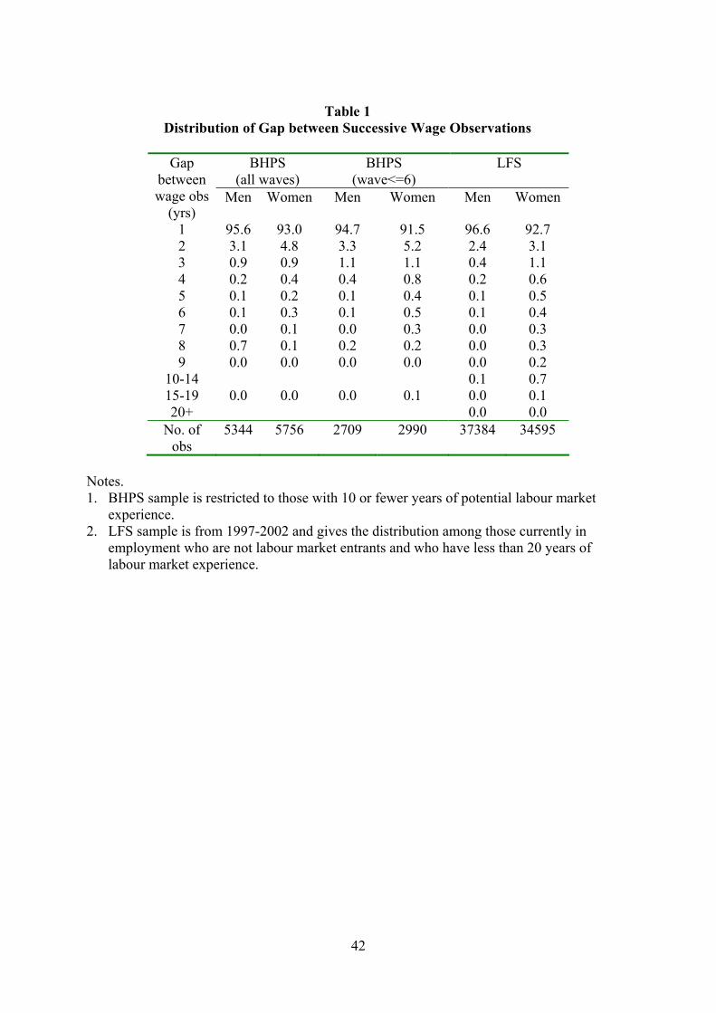
42

Table 1

Distribution of Gap between Successive Wage Observations

BHPS (all waves)

BHPS (wave<=6)

LFS Gap between wage obs

(yrs) Men Women Men Women Men Women

1 95.6 93.0 94.7 91.5 96.6 92.7 2 3.1 4.8 3.3 5.2 2.4 3.1 3 0.9 0.9 1.1 1.1 0.4 1.1 4 0.2 0.4 0.4 0.8 0.2 0.6 5 0.1 0.2 0.1 0.4 0.1 0.5 6 0.1 0.3 0.1 0.5 0.1 0.4 7 0.0 0.1 0.0 0.3 0.0 0.3 8 0.7 0.1 0.2 0.2 0.0 0.3 9 0.0 0.0 0.0 0.0 0.0 0.2

10-14 0.1 0.7 15-19 0.0 0.1 20+

0.0

0.0

0.0

0.1

0.0 0.0 No. of

obs 5344 5756 2709 2990 37384 34595

Notes. 1. BHPS sample is restricted to those with 10 or fewer years of potential labour market

experience. 2. LFS sample is from 1997-2002 and gives the distribution among those currently in

employment who are not labour market entrants and who have less than 20 years of labour market experience.

43

Table 2 ‘Reduced Form’ Estimates of Wage Growth Equation

1 2 3 4 5 6 Men Women Men Women Men Women

0 yrs of experience

0.145 (0.013)

0.120 (0.012)

0.161 (0.013)

0.131 (0.011)

0.160 (0.019)

0.160 (0.016)

5 yrs of

experience 0.068

(0.005) 0.040

(0.004) 0.070

(0.004) 0.046

(0.004) 0.074

(0.008) 0.041

(0.006)

10 yrs of experience

0.013 (0.010)

0.009 (0.006)

0.030 (0.007)

0.035 (0.007)

0.018 (0.015)

0.020 (0.011)

No. of obs 5015 5535 4833 5208 5015 5535

R2 0.076 0.051 0.077 0.058 0.020 0.015 Fixed Effects No No No No Yes

P=1.00 Yes

P=1.00 Sample All All Gap=1 Gap=1 All All

Implied Gender

Gap at 5 yrs 0.144

(0.044) 0.149

(0.041) 0.096

(0.062) Implied Gender Gap at 10 yrs

0.248 (0.054)

0.222 (0.044)

0.216 (0.066)

Notes. 1. These estimates are derived from the estimation of (4) where experience is modeled as

a quadratic. 2. Standard errors in parentheses. These are robust standard errors with clustering on the

individual.

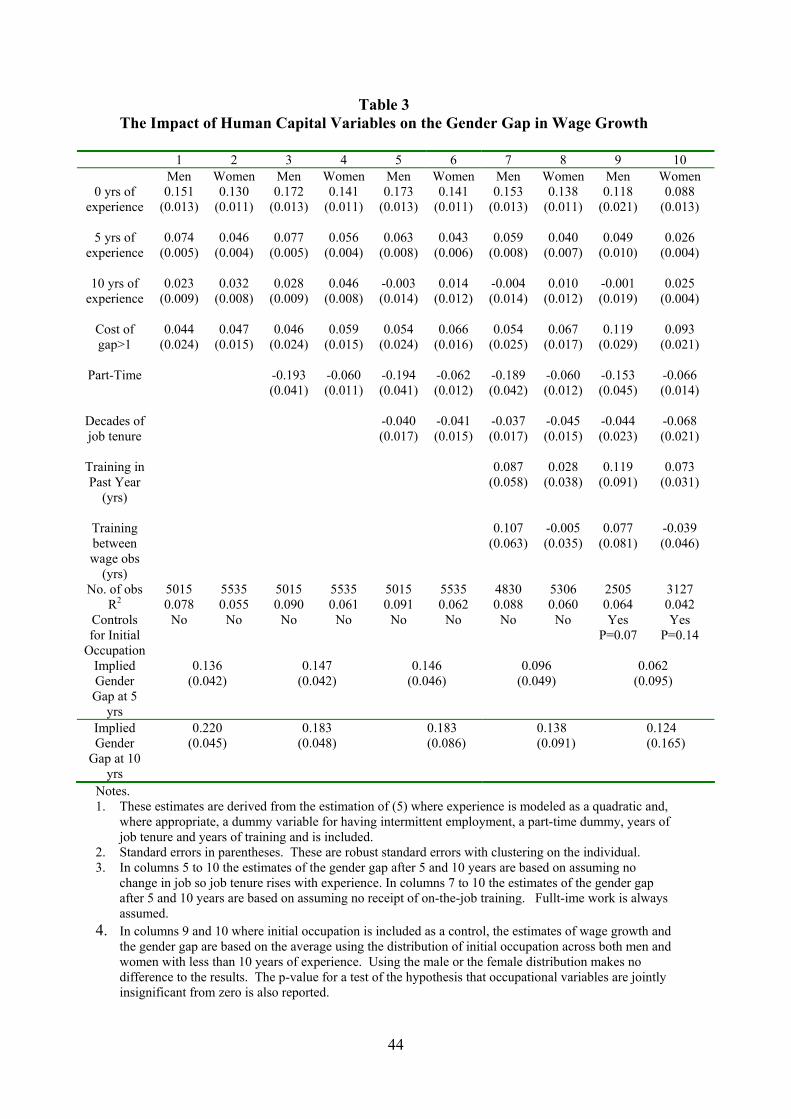
44

Table 3 The Impact of Human Capital Variables on the Gender Gap in Wage Growth

1 2 3 4 5 6 7 8 9 10 Men Women Men Women Men Women Men Women Men Women

0 yrs of experience

0.151 (0.013)

0.130 (0.011)

0.172 (0.013)

0.141 (0.011)

0.173 (0.013)

0.141 (0.011)

0.153 (0.013)

0.138 (0.011)

0.118 (0.021)

0.088 (0.013)

5 yrs of

experience 0.074

(0.005) 0.046

(0.004) 0.077

(0.005) 0.056

(0.004) 0.063

(0.008) 0.043

(0.006) 0.059

(0.008) 0.040

(0.007) 0.049

(0.010) 0.026

(0.004)

10 yrs of experience

0.023 (0.009)

0.032 (0.008)

0.028 (0.009)

0.046 (0.008)

-0.003 (0.014)

0.014 (0.012)

-0.004 (0.014)

0.010 (0.012)

-0.001 (0.019)

0.025 (0.004)

Cost of gap>1

0.044 (0.024)

0.047 (0.015)

0.046 (0.024)

0.059 (0.015)

0.054 (0.024)

0.066 (0.016)

0.054 (0.025)

0.067 (0.017)

0.119 (0.029)

0.093 (0.021)

Part-Time -0.193

(0.041) -0.060 (0.011)

-0.194 (0.041)

-0.062 (0.012)

-0.189 (0.042)

-0.060 (0.012)

-0.153 (0.045)

-0.066 (0.014)

Decades of job tenure

-0.040 (0.017)

-0.041 (0.015)

-0.037 (0.017)

-0.045 (0.015)

-0.044 (0.023)

-0.068 (0.021)

Training in Past Year

(yrs)

0.087 (0.058)

0.028 (0.038)

0.119 (0.091)

0.073 (0.031)

Training between wage obs

(yrs)

0.107 (0.063)

-0.005 (0.035)

0.077 (0.081)

-0.039 (0.046)

No. of obs 5015 5535 5015 5535 5015 5535 4830 5306 2505 3127 R2 0.078 0.055 0.090 0.061 0.091 0.062 0.088 0.060 0.064 0.042

Controls for Initial

Occupation

No No No No No No No No Yes P=0.07

Yes P=0.14

Implied Gender Gap at 5

yrs

0.136 (0.042)

0.147 (0.042)

0.146 (0.046)

0.096 (0.049)

0.062 (0.095)

Implied Gender

Gap at 10 yrs

0.220 (0.045)

0.183 (0.048)

0.183 (0.086)

0.138 (0.091)

0.124 (0.165)

Notes. 1. These estimates are derived from the estimation of (5) where experience is modeled as a quadratic and,

where appropriate, a dummy variable for having intermittent employment, a part-time dummy, years of job tenure and years of training and is included.

2. Standard errors in parentheses. These are robust standard errors with clustering on the individual. 3. In columns 5 to 10 the estimates of the gender gap after 5 and 10 years are based on assuming no

change in job so job tenure rises with experience. In columns 7 to 10 the estimates of the gender gap after 5 and 10 years are based on assuming no receipt of on-the-job training. Fullt-ime work is always assumed.

4. In columns 9 and 10 where initial occupation is included as a control, the estimates of wage growth and the gender gap are based on the average using the distribution of initial occupation across both men and women with less than 10 years of experience. Using the male or the female distribution makes no difference to the results. The p-value for a test of the hypothesis that occupational variables are jointly insignificant from zero is also reported.

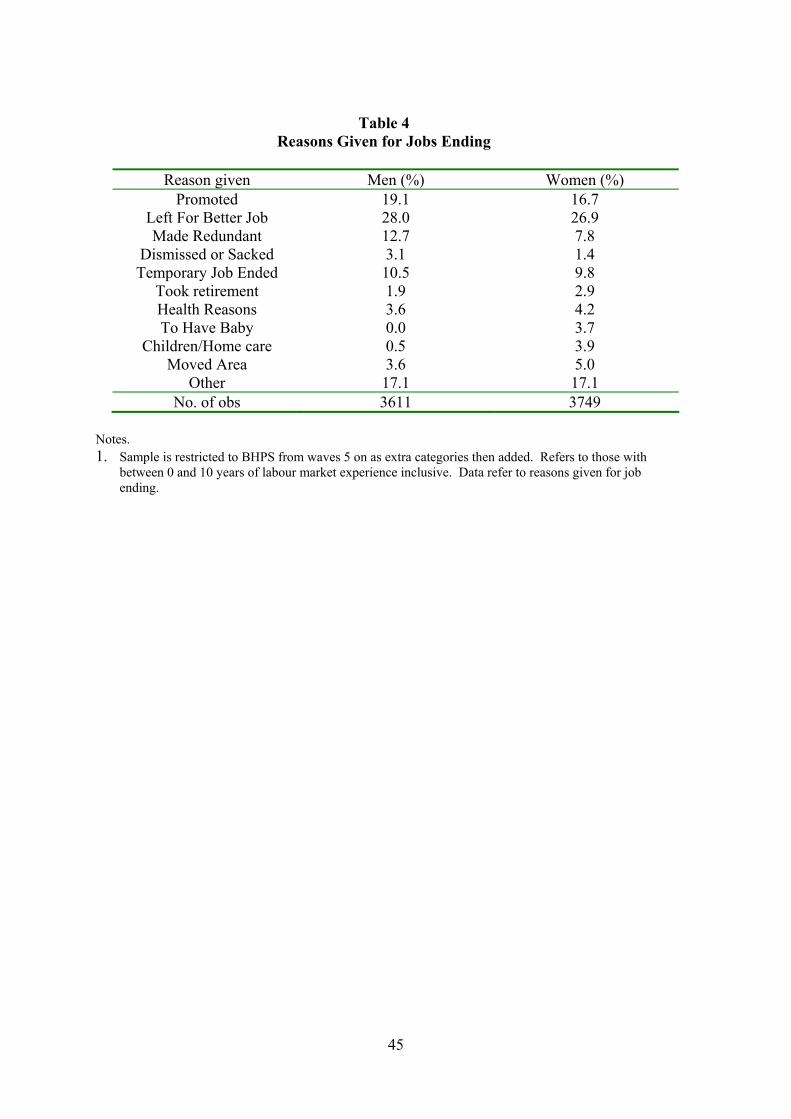
45

Table 4

Reasons Given for Jobs Ending

Reason given Men (%) Women (%) Promoted 19.1 16.7

Left For Better Job 28.0 26.9 Made Redundant 12.7 7.8

Dismissed or Sacked 3.1 1.4 Temporary Job Ended 10.5 9.8

Took retirement 1.9 2.9 Health Reasons 3.6 4.2 To Have Baby 0.0 3.7

Children/Home care 0.5 3.9 Moved Area 3.6 5.0

Other 17.1 17.1 No. of obs 3611 3749

Notes. 1. Sample is restricted to BHPS from waves 5 on as extra categories then added. Refers to those with

between 0 and 10 years of labour market experience inclusive. Data refer to reasons given for job ending.

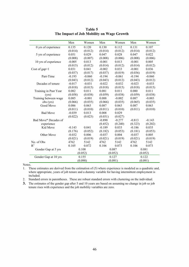
46

Table 5

The Impact of Job Mobility on Wage Growth

Men Women Men Women Men Women 0 yrs of experience 0.135

(0.014) 0.120 (0.012)

0.130 (0.014)

0.112 (0.012)

0.131 (0.014)

0.107 (0.012)

5 yrs of experience 0.051 (0.008)

0.029 (0.007)

0.047 (0.008)

0.028 (0.006)

0.047 (0.008)

0.022 (0.006)

10 yrs of experience -0.005 (0.015)

0.013 (0.012)

-0.001 (0.014)

0.013 (0.012)

-0.001 (0.014)

0.005 (0.012)

Cost of gap>1 0.031 (0.037)

0.041 (0.017)

-0.002 (0.037)

0.033 (0.019)

-0.001 (0.036)

0.036 (0.019)

Part-Time -0.193 (0.043)

-0.060 (0.012)

-0.194 (0.043)

-0.061 (0.012)

-0.194 (0.043)

-0.060 (0.012)

Decades of tenure -0.017 (0.018)

-0.031 (0.015)

-0.022 (0.018)

-0.032 (0.015)

-0.023 (0.018)

-0.033 (0.015)

Training in Past Year (yrs)

0.082 (0.058)

0.011 (0.038)

0.081 (0.059)

0.011 (0.038)

0.080 (0.059)

0.011 (0.038)

Training between wage obs (yrs)

0.085 (0.066)

-0.001 (0.035)

0.088 (0.066)

-0.002 (0.035)

0.087 (0.065)

-0.003 (0.035)

Good Move

0.086 (0.011)

0.063 (0.010)

0.087 (0.011)

0.063 (0.010)

0.087 (0.011)

0.063 (0.010)

Bad Move

-0.039 (0.022)

0.013 (0.023)

0.008 (0.031)

0.029 (0.027)

Bad Move* Decades of experience

-0.890 (0.452)

-0.277 (0.240)

-0.813 (0.323)

-0.143 (0.202)

Kid Move

-0.143 (0.176)

0.041 (0.052)

-0.189 (0.182)

0.033 (0.053)

-0.186 (0.181)

0.035 (0.053)

Other Move

-0.032 (0.021)

0.006 (0.019)

-0.037 (0.021)

0.004 (0.019)

-0.037 (0.021)

0.005 (0.019)

No. of Obs 4762 5142 4762 5142 4762 5142 R2 0.105 0.072 0.106 0.073 0.106 0.073

Gender Gap at 5 yrs 0.108 (0.052)

0.087 (0.052)

0.081 (0.052)

Gender Gap at 10 yrs 0.155 (0.090)

0.127 (0.091)

0.122 (0.091)

Notes. 1. These estimates are derived from the estimation of (5) where experience is modeled as a quadratic and,

where appropriate, years of job tenure and a dummy variable for having intermittent employment is included.

2. Standard errors in parentheses. These are robust standard errors with clustering on the individual. 3. The estimates of the gender gap after 5 and 10 years are based on assuming no change in job so job

tenure rises with experience and the job mobility variables are zero.

47

Table 6 Gender Differences in Personality Among Teenagers: BHPS Data

Percentages agreeing with the statement Men Women Sample I feel I have a number of good qualities 93.0 91.0 1,883 (1,882) I feel that I do not have much to be proud of 13.9 17.5 1,883 (1,882) I certainly feel useless at times 29.1 44.8 3,948 (3,753) I am able to do things as well as most other people

91.0 90.5 1,883 (1,882)

I am a likeable person 93.0 93.6 3,948 (3,753) I can usually solve my own problems 90.2 86.0 1,883 (1,882) All in all, I am inclined to feel I am a failure 8.9 12.1 3,948 (3,753) At times I feel I am no good at all 22.6 35.3 3,948 (3,753) I feel left out of things when I am with friends

15.6 25.0 2,752 (2,679)

Notes: 1. In the final column female sample sizes are shown in the parentheses. 2. Rows 1,2,4 and 6 includes BHPS waves 9-11. Rows 3,5, and 7 includes BHPS waves 4-11. Row 9

includes BHPS waves 7-11. ‘Agree” includes strongly agree and agree.

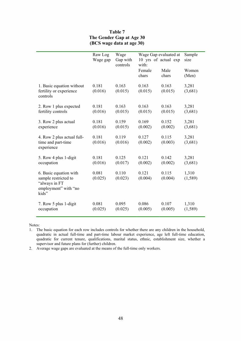
48

Table 7 The Gender Gap at Age 30 (BCS wage data at age 30)

Raw Log

Wage gap Wage Gap with controls

Wage Gap evaluated at 10 yrs of actual exp with:

Sample size

Female

chars Male chars

Women (Men)

1. Basic equation without fertility or experience controls

0.181 (0.016)

0.163 (0.015)

0.163 (0.015)

0.163 (0.015)

3,281 (3,681)

2. Row 1 plus expected fertility controls

0.181 (0.016)

0.163 (0.015)

0.163 (0.015)

0.163 (0.015)

3,281 (3,681)

3. Row 2 plus actual experience

0.181 (0.016)

0.159 (0.015)

0.169 (0.002)

0.152 (0.002)

3,281 (3,681)

4. Row 2 plus actual full-time and part-time experience

0.181 (0.016)

0.119 (0.016)

0.127 (0.002)

0.115 (0.003)

3,281 (3,681)

5. Row 4 plus 1-digit occupation

0.181 (0.016)

0.125 (0.017)

0.121 (0.002)

0.142 (0.002)

3,281 (3,681)

6. Basic equation with sample restricted to “always in FT employment” with “no kids”

0.081 (0.025)

0.110 (0.023)

0.121 (0.004)

0.115 (0.004)

1,310 (1,589)

7. Row 5 plus 1-digit occupation

0.081 (0.025)

0.095 (0.025)

0.086 (0.005)

0.107 (0.005)

1,310 (1,589)

Notes: 1. The basic equation for each row includes controls for whether there are any children in the household,

quadratic in actual full-time and part-time labour market experience, age left full-time education, quadratic for current tenure, qualifications, marital status, ethnic, establishment size, whether a supervisor and future plans for (further) children.

2. Average wage gaps are evaluated at the means of the full-time only workers.

49

Table 8 Gender Differences in Personality Among Children: BCS Data

Self-esteem Difference in means (standard

error)

Locus of control Difference in means (standard

error) Female Male Female Male Age 10 scores (sample = age 10 and age 30 respondents)

-0.025 0.153 0.178 (0.028)*

0.108 0.119 0.011 (0.028)

Sample sizes 2,345 2,620 2,345 2,620 Age 16 scores (sample = age 16 and age 30 respondents)

0.087 0.123 0.036 (0.046)

0.094 0.110 0.016 (0.042)

Sample sizes 1,111 879 1,111 879 Sample of age 10, 16 and 30 respondents

Age 10 scores -0.010 0.269 0.278 (0.050)*

0.215 0.326 0.111 (0.049)

Age 16 scores 0.097 0.143 0.046 (0.053)

0.111 0.150 0.039 (0.048)

Sample sizes 835 638 835 638 Notes:

1. * indicates statistically significant at 1%. 2. The self-esteem and locus of control figures presented above are standardized versions of the

original score variables.

50

Table 9

Coefficient estimates for the self-esteem and locus of control scores in the wage equation

(BCS wage data at age 30)

Self-esteem coefficient estimates

Locus of control coefficient estimates

Sample size

Women Men Women Men Women

(Men) 1. Basic wage equation on sample of age 30 and 10 respondents plus self-esteem and locus of control from age 10

0.031 (0.014)

0.009 (0.014)

0.051 (0.016)

0.058 (0.014)

2,345 (2,620)

2. Basic wage equation on sample of age 30 and 16 respondents plus self-esteem and locus of control age 16

0.030 (0.022)

0.031 (0.023)

0.067 (0.025)

0.032 (0.027)

1,111 (879)

3. Basic wage equation on sample of age 30, 16 and 10 respondents plus self-esteem and locus of control from age 10

0.056 (0.026)

0.007 (0.030)

0.066 (0.029)

0.078 (0.031)

835 (638)

Notes: 1. The basic equation for each row includes controls for whether there are any children in the household,

quadratic in actual full-time and part-time labour market experience, age left full-time education, quadratic for current tenure, qualifications, marital status, ethnic, establishment size, whether a supervisor and future plans for (further) children.

2. The sample in row 1 is BCS at age 30 merged with the BCS age 10 sample. The sample in row 2 is the BCS at age 30 merged with BCS age 16 sample. The sample in row 3 is the BCS at age 30 merged with the BCS age 10 and 16 samples.

3. Standard errors in parentheses in columns 2-5.

51

Table 10

Impact of self-esteem and locus of control scores on the gender gap (BCS wage data at age 30)

Raw Log

Wage gap Wage Gap with controls

Wage Gap evaluated at 10 yrs of actual exp with±:

Sample size

Female

chars Male chars

Female (Male)

1. Basic wage equation on sample of age 30 and 10 respondents

0.188 (0.019)

0.128 (0.019)

0.133 (0.002)

0.120 (0.002)

2,345 (2,620)

2. Equation and sample as row above plus self-esteem and locus of control scores from age 10

0.188 (0.019)

0.124 (0.019)

0.130 (0.002)

0.115 (0.002)

2,345 (2,620)

3. Basic wage equation on sample of age 30 and 16 respondents

0.155 (0.031)

0.083 (0.031)

0.057 (0.005)

0.048 (0.005)

1,111 (879)

4. Equation and sample as row above plus self-esteem and locus of control from age 16

0.155 (0.031)

0.083 (0.031)

0.058 (0.005)

0.047 (0.005)

1,111 (879)

5. Basic wage equation on sample of age 30, 16 and 10 respondents

0.176 (0.036)

0.110 (0.035)

0.089 (0.006)

0.096 (0.005)

835 (638)

6. Equation and sample as row above plus self-esteem and locus of control from age 10

0.176 (0.036)

0.097 (0.036)

0.082 (0.006)

0.076 (0.006)

835 (638)

Notes: 1. The basic equation for each row includes controls for whether there are any children in the household,

quadratic in actual full-time and part-time labour market experience, age left full-time education, quadratic for current tenure, qualifications, marital status, ethnic, establishment size, whether a supervisor and future plans for (further) children.

2. The sample in rows 1 and 2 is BCS at age 30 merged with the BCS age 10 sample. The sample in rows 3 and 4 is BCS at age 30 merged with BCS age 16 sample. The sample in rows 5 and 6 is BCS at age 30 merged with the BCS age 10 and 16 samples.

3. Standard errors in parentheses in columns 2-5. 4. ± denotes that the average wage gaps are evaluated at the means of the full-time only workers.

52

Table A1 Summary Statistics for BHPS Data

Young Workers

(<10 yrs of potential experience) Men Women

Log Wage Growth 0.084 (0.306)

0.065 (0.278)

Potential experience (decades) 0.48 (0.28)

0.47 (0.28)

Job Tenure (decades) 0.15 (0.22)

0.13 (0.19)

Gap between wage obs 1.02 (0.18)

1.02 (0.18)

Part-Time 0.036 0.196 Training in Past Year (yrs) 0.035

(0.106) 0.030

(0.095) Training between wage obs (yrs) 0.030

(0.090) 0.030

(0.099) Good Move 0.254 0.231 Bad Move 0.072 0.056 Kid Move 0.0005 0.010

Other Move 0.062 0.072 Manager 0.035 0.036

Professional occupations 0.060 0.049 Associate professional 0.104 0.104

Administrative and secretarial 0.156 0.378 Skilled trades 0.239 0.022

Personal services 0.083 0.200 Sales/customer services 0.081 0.109

Machine operatives 0.094 0.037 Elementary 0.147 0.068 Graduates 0.283 0.290 `A’ Level 0.396 0.430 GSCEs 0.286 0.267

No qualifications 0.036 0.012 Black 0.011 0.010 Asian 0.025 0.010

Married 0.442 0.543 Child in Household 0.253 0.259

No. of kids 0-2 0.098 0.070 No. of kids 3-4 0.051 0.066

No. of kids 12-15 0.107 0.099 No. of kids 16-18 0.028 0.031

Notes. 1. Sample is those with observations on wage growth aged 16-65 with less than 45 years of

potential experience. Sample numbers for wage growth are 5015 for men and 5535 for women – some variables have smaller sample sizes because of non-response.

2. Means are reported and standard errors in parentheses. Standard errors not reported for binary variables.

53

Figure 1 The Earnings-Experience Profile for Men and Women

0.2

.4.6

.8lo

g ho

urly

wag

es

0 10 20 30 40 50exp

male femaledifference

Notes. 1. Data come from the first 12 waves of the BHPS. 2. Log hourly wages are normalized to be zero for men with zero years of labour market experience.

Figure 2 The Evolution of the Gender Pay Gap for Different Birth Cohorts

0.2

.4.6

gend

er w

age

gap

(log

poin

ts)

20 30 40 50 60age

Born 1938-1942 Born 1948-1952Born 1958-1962 Born 1968-1972Born 1975-1979

Notes. 1. Data come from the New Earnings Survey, 1975-2001. 2. Earnings data are hourly earnings excluding over-time.

54

Figure 3

Gender Differences in Wage Growth: New Earnings Survey Data

0.0

5.1

.15

.2

15 20 25 30 35age

Male Wage GrowthFemale Wage GrowthGender Gap in Wage Growth

Notes. 1. The NES does not contain information on education so cannot be used to compute years of experience. 2. This is annual wage growth for the sample of workers observed in two adjacent years.

Figure 4

Gender Differences in Accumulated Work Experience

05

1015

20m

onth

s

1 2 3 4 5 6 7 8 9 10potential experience (years)

gender gap in actual experiencegender gap in FT actual experiencegender gap in actual experience for workersgender gap in FT actual experience for workers

Notes. 1. These figures come from the 1970 British Cohort Study. I would like to thank Fernando Galindo-Rueda

for allowing me to use the work-history data he had constructed.

55

Figure 5

Gender Differences in On-the-Job Training

-.04

-.02

0.0

2.0

4.0

6G

ende

r Gap

in J

ob-R

elat

ed T

rain

ing

(Yea

rs)

0 5 10 15 20years of potential experience

AllSchool Leaving Age <=17School Leaving Age >=18 and <=20School Leaving Age >=21

Notes.

1. This data comes from the Labour Force Survey for the years 2000-2003.

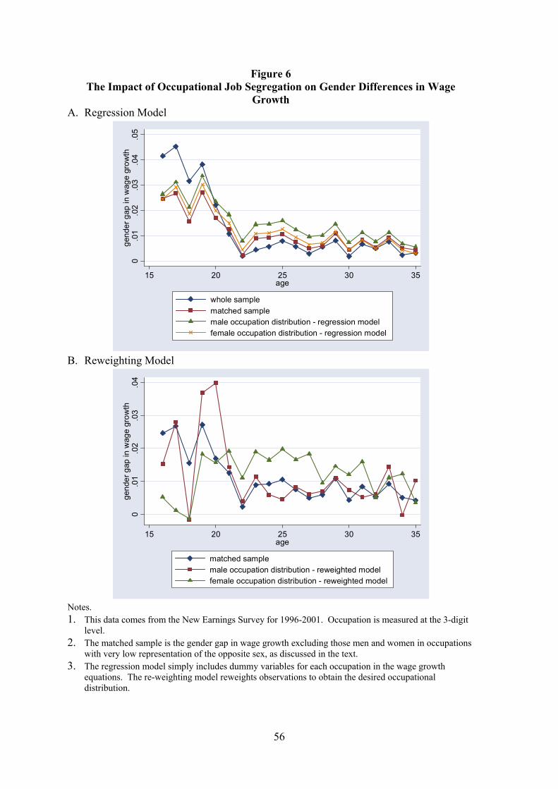
56

Figure 6 The Impact of Occupational Job Segregation on Gender Differences in Wage

Growth A. Regression Model

0.0

1.0

2.0

3.0

4.0

5ge

nder

gap

in w

age

grow

th

15 20 25 30 35age

whole samplematched samplemale occupation distribution - regression modelfemale occupation distribution - regression model

B. Reweighting Model

0.0

1.0

2.0

3.0

4ge

nder

gap

in w

age

grow

th

15 20 25 30 35age

matched samplemale occupation distribution - reweighted modelfemale occupation distribution - reweighted model

Notes. 1. This data comes from the New Earnings Survey for 1996-2001. Occupation is measured at the 3-digit

level. 2. The matched sample is the gender gap in wage growth excluding those men and women in occupations

with very low representation of the opposite sex, as discussed in the text. 3. The regression model simply includes dummy variables for each occupation in the wage growth

equations. The re-weighting model reweights observations to obtain the desired occupational distribution.

57

Figure 7

Job Mobility Rates: Total

.2.3

.4.5

.6.7

Mob

ility

Rat

e

0 5 10 15 20Years of Potential Experience

Men Women

Notes. 1. These data come from the BHPS. 2. The mobility rate is measured as the fraction of workers who change jobs or leave a job for non-

employment in the coming year.

Figure 8 Job Mobility Rates: for better job

.1.1

5.2

.25

.3.3

5M

obili

ty R

ate

0 5 10 15 20Years of Potential Experience

Men Women

Notes. 1. As for Figure 7 but with mobility defined as being for a better job.

58

Figure 9

Job Mobility Rates: not for better job

.1.1

5.2

.25

.3M

obili

ty R

ate

0 5 10 15 20Years of Potential Experience

Men Women

Notes. 1. As for Figure 7 but with mobility not being defined as being for a better job.

CENTRE FOR ECONOMIC PERFORMANCE Recent Discussion Papers

699 Andrew B. Bernard Stephen Redding Peter K. Schott

Products and Productivity

698 Nicholas Oulton Ex Post Versus Ex Ante Measures of the User Cost of Capital

697 Alan Manning You Can’t Always Get What You Want: the Impact of the Jobseeker’s Allowance

696 Andrew B. Bernard Stephen Redding Peter K. Schott

Factor Price Equality and the Economies of the United States

695 Henry G. Overman Anthony J. Venables

Cities in the Developing World

694 Carlo Rosa Giovanni Verga

The Importance of the Wording of the ECB

693 Richard Dickens Mirko Draca

The Employment Effects of the October 2003 Increase in the National Minimum Wage

692 Ralf Martin Computing the True Spread

691 Augustin de Coulon François-Charles Wolff

Immigrants at Retirement: Stay/Return or ‘Va-et-Vient’?

690 Monika Merz Eran Yashiv

Labor and the Market Value of the Firm

689 Pierre-Philippe Combes Giles Duranton Henry G. Overman

Agglomeration and the Adjustment of the Spatial Economy

688 Stephen Redding Daniel M. Sturm

The Costs of Remoteness: Evidence from German Division and Reunification

687 Vicente Cuñat Maria Guadalupe

How Does Product Market Competition Shape Incentive Contracts?

686 Maria Guadalupe Product Market Competition, Returns to Skill and Wage Inequality

685 Jo Blanden Stephen Machin John Van Reenen

New Survey Evidence on Recent Changes in UK Union Recognition

684 Giovanna Vallanti Capital Mobility and Unemployment Dynamics: Evidence from a Panel of OECD Countries

683 Gilles Duranton Michael Storper

Rising Trade Costs? Agglomeration and Trade with Endogenous Transaction Costs

682 Carlo Rosa Giovanni Verga

Is ECB Communication Effective?

681 Nicholas Oulton Sylaja Srinivasan

Productivity Growth and the Role of ICT in the United Kingdom: An Industry View, 1970-2000

680 Stephen Machin Olivier Marie

Crime and Police Resources: the Street Crime Initiative

679 Alan Manning Barbara Petrongolo

The Part-Time Pay Penalty

678 Andrew Clark Fabien Postel-Vinay

Job Security and Job Protection

677 Eran Yashiv Evaluating the Performance of the Search and Matching Model

676 Alex Bryson Rafael Gomez Tobias Kretschmer

Catching a Wave: the Adoption of Voice and High Commitment Workplace Practices in Britain: 1984-1998

675 Nick Bloom Mark Schankerman John Van Reenen

Identifying Technology Spillovers and Product Market Rivalry

The Centre for Economic Performance Publications Unit Tel 020 7955 7673 Fax 020 7955 7595 Email info@cep.lse.ac.uk

Web site http://cep.lse.ac.uk