Economics Working Paper Series

Working Paper 09/118August 2009

Hans Gersbach, Gerhard Sorger and Christian Amon

Hierarchical Growth: Basic and Applied Research

CER-ETH – Center of Economic Research at ETH Zurich

Hierarchical Growth: Basic and Applied Research∗

Hans Gersbach

CER-ETH Center of Economic Research

at ETH Zurich and CEPR

8032 Zurich, Switzerland

hgersbach@ethz.ch

Gerhard Sorger

Department of Economics

University of Vienna

1010 Vienna, Austria

gerhard.sorger@univie.ac.at

Christian Amon

CER-ETH Center of Economic Research

at ETH Zurich

8032 Zurich, Switzerland

camon@ethz.ch

This Version: July 2009

Abstract

We develop a model that incorporates salient features of growth in modern economies.We combine the expanding-variety growth model through horizontal innovations with ahierarchy of basic and applied research. The former extends the knowledge base, whilethe latter commercializes it. Two-way spillovers reinforce the productivity of research ineach sector. We establish the existence of balanced growth paths. Along such paths thestock of ideas and the stock of commercialized blueprints for intermediate goods growwith the same rate. Basic research is a necessary and sufficient condition for economicgrowth. We show that there can be two different facets of growth in the economy.First, growth may be entirely shaped by investments in basic research if applied researchoperates at the knowledge frontier. Second, long-run growth may be shaped by bothbasic and applied research and growth can be further stimulated by research subsidies.We illustrate different types of growth processes by examples and polar cases when onlyupward or downward spillovers between basic and applied research are present.

Keywords: Basic research, applied research, knowledge base, commercialization, hi-erarchical economic growth

JEL Classification: H41, O31, O41

∗We would like to thank Maik Schneider, Ralph Winkler and seminar participants at ETH Zurich for valu-able comments and suggestions.

1

“It is likely that the bulk of the economic benefits of university research come from inven-tions in the private sector that build upon the scientific and engineering base created by uni-versity research, rather than from commercial inventions generated directly by universities.”[Henderson et al. (1998), p. 126]

1 Introduction

The innovation processes in both industrialized and industrializing countries are typicallycharacterized by a hierarchy of basic and applied research. Basic research is mainly publiclyfunded and extends the knowledge base of an economy by generating novel ideas, theories,and prototypes that are usually of no immediate commercial use. Applied research, on theother hand, is primarily carried out by private firms, which commercialize the output of basicresearch by transforming it into blueprints for new products. Moreover, basic and appliedresearch reinforce each other throughout the entire process of knowledge base extensionand commercialization. For example, applied research benefits from basic research becausethe latter provides knowledge and methods that support the problem-solving processes atresearch-active private firms, whereas basic research benefits from applied research as thelatter identifies unresolved problems and discovers new challenges for basic research. Thatis, the innovation process is characterized by two-way spillovers between basic and appliedresearch.

This paper develops an endogenous growth model that captures the above hierarchy and in-terdependency of the innovation process. We analyze a closed economy with a final and anintermediate goods sector, a basic and an applied research sector, a continuum of infinitelylived households, and a government. Technological progress is the result of a hierarchicalinnovation process modelled along the lines sketched above: basic research is financed bythe government and extends the knowledge base of the economy, whereas applied researchis carried out by private firms that transform basic knowledge into blueprints for new inter-mediate goods. In addition, two-way spillovers between basic and applied research reinforcethe productivity in each research sector. In this setup, the government can influence growthand welfare of the economy by choosing the size of the basic research sector and by grantingsubsidies to researchers. Both of these government activities are financed by taxes on laborincome.

Our model stands in the tradition of the expanding-variety framework of growth throughhorizontal innovations initiated by Romer (1990).1 The crucial features of our model are thehierarchy in the innovation process and the two-way spillovers between basic and appliedresearch as described above. While Romer and others effectively assumed an exogenous,

1See Gancia and Zilibotti (2005) for a recent review of the development, extensions, and applications ofthe expanding-variety framework.

2

non-exhaustible pool of knowledge available that can be exploited by applied researchersto invent blueprints for new intermediate goods, we endogenize this knowledge pool as theoutput of a basic research sector. In other words, we assume that the productivity of appliedresearch is constrained by the “knowledge frontier” of the economy which, in turn, can onlybe pushed outwards by basic research. In particular, growth is about to cease in the long-rununless the knowledge base of the economy is permanently expanded by basic research.

We establish the existence of balanced growth paths. Along such paths the stock of ideas andthe stock of commercialized blueprints for intermediate goods grow with the same rate. Ba-sic research is a necessary and sufficient condition for economic growth. We show that therecan be two different facets of growth in the economy. First, growth may be entirely shapedby investments in basic research if applied research operates at the knowledge frontier. Sec-ond, long-run growth may be shaped by both basic and applied research and growth can befurther stimulated by research subsidies. We illustrate different types of growth processesby examples and polar cases when only upward or downward spillovers are present. In theformer case, a higher share of labor employed in basic research translates into higher growthrates and applied research operates at the knowledge frontier. In the latter case, growth isdeclining if basic research exceeds a certain threshold and ceases entirely if basic research isincreased further as undertaking applied research becomes unprofitable.

So far, only few attempts have been made to analyze the impact of publicly-funded basicresearch in a dynamic setup. Among the first were Shell’s (1966, 1967) contributions, whichhighlight the necessity of allocating economic resources to the process of invention. Thereby,Shell’s concept of technical knowledge, which he treats as a public good financed solely bymeans of output taxes, corresponds closely to our notion of basic research. Similarly, Gross-man and Helpman (1991) address the positive impact on growth of basic research financedby means of income taxes vis-a-vis the negative effect caused by the associated tax distor-tions. In order to evaluate the impact of various research policies, Morales (2004) considersan endogenous growth model of vertical innovation incorporating both basic and appliedresearch performed by both private firms and the government. While these and other contri-butions shed light on the positive impact of publicly-funded basic research on growth, theydo neither consider the hierarchy of basic and applied research nor the two-way spilloversbetween the two types of research in the process of innovation. Our formulation of two-wayspillovers between basic and applied research follows the description of Park (1998).

The paper is organized as follows. In the following section we present empirical supportfor our central assumptions regarding the hierarchy and the presence of two-way spilloversin the innovation process. Section 3 sets up the formal model. In Section 4 we defineand characterize the competitive equilibrium corresponding to a fixed policy scheme of thegovernment. We identify the determinants of economic growth. In Section 5 we focus on thepolar cases of upward and downward spillovers between basic and applied research. Section

3

7 concludes. All proofs are collected in an appendix.

2 Empirical motivation

In this section we motivate our analysis by several empirical observations. More specifically,we document the fact that basic research is primarily government-funded whereas appliedresearch is typically carried out by private firms, and we demonstrate the hierarchy betweenbasic and applied research as well as the existence of two-way spillovers.

2.1 Shares of basic and applied research in GDP and modes of financ-ing

Basic and applied research expenditures constitute significant shares of GDP in most indus-trialized and industrializing countries. As Table 1 shows, in 2006 the average ratio of totalR&D expenditures to GDP in a sample of countries with comparable data was 2.01 percentwith the lowest ratio in Argentina (0.50) and the highest in Israel (4.65). Moreover, theaverage R&D expenditure to GDP ratio increased from 1.77 percent in 2000 to 2.01 per-cent in 2006. On average, basic research expenditures made up 23.07 percent of total R&Dexpenditures in 2006 with the lowest share in China (5.19) and the highest in the Slovak Re-public (45.10). The average share of basic research expenditures in total R&D expendituresincreased from 20.17 percent in 2000 to 23.07 percent in 2006.

While basic research is mainly financed through public funds, applied research is funded andperformed mainly by the private sector as illustrated by Table 2. This table shows the sourcesof funding for basic and applied research in 2006 broken down into government and highereducation institutions, whose research is mainly financed by public funds2, business enter-prises, as well as private non-profit institutions. Table 2 shows that on average 73.76 percentof basic research expenditures were financed and carried out by government and higher ed-ucation institutions, while business enterprises and private non-profit institutions accountedfor 22.36 and 3.89 percent, respectively. Almost the exact opposite pattern holds for thefinancing scheme of applied research. While government and higher education institutionson average financed and performed 24.64 percent of applied research, business enterprisesand private non-profit institutions accounted for 73.73 and 1.63 percent, respectively. Takingthese figures regarding the respective financing shares of basic and applied research into ac-count, we settle on the following use of notation. Basic research corresponds to university oracademic research and science, while applied research is associated with industry research.

2It should be noted here that in some countries income from patenting and licensing of university inventionsbecame an additional source of financing for universities (see, for example, Colyvas et al., 2002, for the caseof the US, particularly after the passage of the Bayh-Dole Act in 1980).

4

Table 1: R&D Expenditures (Source: OECD, Main Science and Technology Indicators)

Gross Domestic Ex-penditures on R&D asa Percentage of GDP

Basic Research Ex-penditures as a Per-centage of Total R&DExpenditures

Applied Research Ex-penditures as a Per-centage of Total R&DExpendituresa

2000 2006 2000 2006 2000 2006

Argentina 0.44 0.50 27.75 28.07 72.25 71.93

Australia 1.51 1.78b 25.81 23.17b 74.19 76.83b

China 0.90 1.42 5.22 5.19 94.78 94.81

Czech Republic 1.21 1.54 23.33 29.32 76.67 70.68

France 2.15 2.11 23.60 23.75b 76.40 76.25b

Hungary 0.78 1.00 27.19 32.96b 72.81 67.04b

Ireland 1.12 1.32 — 23.85 — 76.15

Israel 4.45 4.65 16.99 16.14 83.01 83.86

Japan 3.04 3.39 12.38 11.98b 87.62 88.02b

Korea 2.39 3.23 12.61 15.15 87.39 84.85

Portugal 0.76 0.83 25.05 25.35b 74.95 74.65b

Singapore 1.88 2.31 11.75 18.83b 88.25 81.17b

Slovak Republic 0.65 0.49 25.61 45.10b 74.39 54.90b

Switzerland 2.53 2.90b 27.96 28.70b 72.04 71.30b

United States 2.74 2.62 17.17c 18.52 82.83c 81.48

Average 1.77 2.01 20.17 23.07 79.83 76.93

aThe OECD categorizes R&D into “basic research”, “applied research”, “experimental development” and“not elsewhere classified”. We summarize the last three items under “applied research” as particularly theOECD’s definition of “experimental development”(see, e.g., OECD, 2002) corresponds closely to our definitionof applied research.

bData from 2004cData from 2001

In the following, we use these terms synonymously.

2.2 Basic research extends the knowledge base for applied research

In most cases, the output of basic research is “embryonic” in nature, which means that it iswithout immediate commercial use and requires refinement through applied research beforeit is ready for commercialization. There are numerous prominent examples of breakthroughinventions by basic research across various disciplines that have been taken up and com-mercialized by applied research. The discovery of X-rays in the area of physics and lifesciences, the discovery of penicillin in the field of medicine, the invention of the method

5

Table 2: Financing Shares of Basic and Applied Research by Sector in 2006 (Source:OECD, Main Science and Technology Indicators)

Basic Research Financing Shares (% ofTotal Basic Research Expenditures)

Applied Research Financing Shares (%of Total Applied Research Expendi-tures)a

Governmentand HigherEducation

BusinessEnterprise

PrivateNon-Profit

Governmentand HigherEducation

BusinessEnterprise

PrivateNon-Profit

Argentina 94.61 2.60 2.81 56.42 41.26 2.32

Australia 83.75b 9.94b 6.31b 30.42b 67.46b 2.12b

China 91.28 8.72 0.00 25.51 74.49 0.00

Czech Republic 77.68 22.19 0.15 15.06 84.43 0.52

France 83.11c 14.38c 2.51c 21.55c 77.57c 0.89c

Hungary 95.54c 4.46c 0.00c 39.59c 60.41c 0.00c

Ireland 63.64 36.36 0.00 23.55 76.44 0.00

Israel 70.48 23.95 5.58 9.18 87.59 3.22

Japan 56.98c 40.12c 2.90c 16.88c 81.40c 1.72c

Korea 38.42 60.76 0.82 18.49 80.20 1.30

Portugal 66.94c 14.30c 18.77c 44.28c 46.65c 9.06c

Singapore 61.49c 38.51c 0.00c 26.66c 73.34c 0.00c

Slovak Republic 84.73c 15.27c 0.00c 19.69c 80.14c 0.17c

Switzerland 64.09b 29.52b 6.38b 7.82b 91.54b 0.64b

United States 73.65 14.26 12.09 14.45 83.09 2.46

Average 73.76 22.36 3.89 24.64 73.73 1.63

aAs in Table 1 we summarize the OECD’s notions of “applied research”, “experimental development” and“not elsewhere classified” under our notion of “applied research”.

bData from 2004cData from 2005

of RNA interference for genetics, the derivation of the lifting line theory for aeronautics,or the invention of the method of nuclear fission for nuclear physics, to name only a few.3

They were all invented through basic research at universities or other public research institu-tions, were subsequently further developed and commercialized, and had finally tremendousimpact in particular industries.

The “embryonic” nature of basic research inventions and their crucial importance for givingrise to new technologies across various industries has been widely documented. Zucker etal. (1998) and Owen-Smith et al. (2002), for example, suggest that basic research inventionswere fundamental to the rise and growth of biotechnology industries. Furthermore, Ander-

3Table 3 in the Appendix contains further examples.

6

son (1997) and Hirschel et al. (2004) highlight the importance of breakthrough theories andfindings made through basic research for subsequent developments in aeronautics industries.National Academy of Engineering (2003) report that basic research has made fundamen-tal contributions to network systems and communications, medical devices and equipment,aerospace, transportation, distribution, and logistics services, as well as to financial servicesindustries.

Jensen and Thursby (2001) find that even the vast majority of licensed university inventionswere “embryonic” in nature with more than 75 percent being merely a proof of concept with-out any particular commercial use in mind. At the time of licensing, only 12 percent of alluniversity inventions were ready for commercialization while for only 8 percent their man-ufacturing feasibility was known. These observations lead the authors to conclude that thelargest part of all licensed university inventions required further development and refinement.

A further crucial property of basic research concerns the duration between its origin in thescientific community and its impact on industrial productivity. In this regard, Adams (1990)finds that the expansion of academic knowledge exerts a positive, but lagged impact on tech-nological change and productivity growth. By applying various measures of science within agrowth-accounting framework, his findings suggest that the impact of new academic knowl-edge on industrial productivity does not take place instantaneously, but is rather associatedwith time-lags of about 20 years stemming from the time necessary to search for and adoptuseful scientific knowledge in industry.

These findings suggest a rather strict hierarchy between basic and applied research. The riseand growth of new industries, as well as the associated invention and development of newproducts initially requires substantial basic research efforts to provide the knowledge basewithout a direct commercial use per se, upon which applied research and commercializationin industry can take place. Apart from giving rise to new industries, basic research alsoinduces the invention and commercialization of new products in existing industries.

2.3 Two-way spillovers between basic and applied research

A crucial property of the innovation system is the existence of two-way spillovers betweenbasic and applied research. Nelson (1993) points out that, while science often preceded therise of new technologies, new fields of technology also often induced the rise of new fieldsof science. That is, throughout the entire process of product invention, development, andcommercialization, basic and applied research are interdependent and mutually benefit fromand reinforce each other through various channels and by various means. Examples for thisinterplay between basic and applied research are given, for example, by von Hippel (1988),who describes the initiating role of basic research among others in the invention of nuclearmagnetic resonance and the electromagnetic lens. The subsequent interaction between basic

7

and applied research was crucial in the further development and refinement of the nuclearmagnetic resonance spectrometer and the transmission electron microscope, respectively.That is, the interdependence of basic and applied research and their mutual intensificationis fundamental to the invention, development, and commercialization of new products andtechnologies.

2.3.1 Impact of basic on applied research

Basic research impacts on applied research, for example, through the channels of open sci-ence, such as publications, scientific reports, conferences and public meetings (Cohen etal., 2002), through “embodied knowledge transfer” associated with scientists moving frombasic to applied research (Zellner, 2003), collaborative and contracted research ventures aswell as informal interaction between basic and applied researchers (Cohen et al., 2002), jointindustry-university research centers (Adams et al., 2001), academic consulting (Perkmannand Walsh, 2008), the patenting and licensing of university inventions (Colyvas et al. 2002),or through the creation of new firms as start-ups and spin-offs from universities (Bania et al.,1993).

According to Martin et al. (1996) and Salter and Martin (2001) publicly funded basic re-search impacts on applied research by generating new knowledge and information as dis-cussed in Subsection 2.2, by training and providing skilled graduates, by developing newscientific instrumentation and methodologies, by establishing networks for knowledge dif-fusion, by enhancing problem-solving capacities, and by creating new firms.4 Furthermore,the involvement of academic inventors in the subsequent commercialization of their inven-tions through applied research allows to employ their tacit knowledge and thereby facilitatescommercialization (Zucker et al., 1998, Jensen and Thursby, 2001).

Various studies have shown the positive impact of academic research on applied research.Nelson (1986), Jaffe (1989), Adams (1990), Acs et al. (1992), or Mansfield (1991, 1992,1995, 1998) find a significant and positive impact of academic research on innovative activityacross various industries. Furthermore, Acs et al. (1994) find that it is particularly small firmsthat benefit relatively strongly from university research. In addition, Funk (2002) suggeststhat basic research generates particularly strong international spillovers.

2.3.2 Impact of applied on basic research

Basic research benefits from applied research, for example, through allowing scientists to ac-cess data, instrumentation, and research material as well as to discover unresolved problems

4Similarly, Mowery and Sampat (2005) suggest that universities provide, for example, new scientific andtechnological knowledge, scientific equipment and instrumentation, prototypes for new products and processes,networks for knowledge diffusion, as well as skilled graduates and faculty.

8

and open challenges when performing academic consulting to industry (Mansfield, 1995,Perkmann and Walsh, 2008). Applied research might also provide basic researchers withknowledge about novel research techniques and methodologies. Furthermore, Adams et al.(2001) suggest that joint industry-university research centers could impact positively on ba-sic research if the associated provision of additional faculty more than compensates for thediversion of faculty resources away from basic and towards applied research. In addition,Agrawal and Henderson (2002) suggest that basic research might also benefit from appliedresearch through increased patenting activities of university faculty.

3 Model formulation

We consider a continuous-time model of an economy that lasts from t = 0 to t = +∞. Theeconomy has one production sector for a final consumption good and one production sectorin which a range of differentiated intermediate goods are produced. In addition, there existtwo R&D sectors. Basic research, which is funded exclusively by the government, generatesideas, theories, and prototypes and thereby extends the economy’s knowledge base. Appliedresearch, on the other hand, is carried out by private researchers who commercialize theoutput of basic research by transforming it into blueprints for new intermediate goods. Theseblueprints are protected by everlasting patents so that the intermediate goods sector operatesunder monopolistic competition. In order to simplify the exposition, we shall henceforthrefer to the output of basic and applied research as ideas and blueprints, respectively.

3.1 Households

The economy is populated by a continuum of measure L > 0 of identical infinitely-livedhouseholds. There is no population growth, that is, L is a constant. The representativehousehold derives utility from consumption according to the utility functional

∫ +∞

0

e−ρt ln[c(t)]dt, (1)

where c(t) denotes per-capita consumption in period t. The parameter ρ > 0 is the commontime-preference rate of the households. Each household is endowed with one unit of homo-geneous labor per unit of time, which can be used for applied research, for basic research,in intermediate goods production, or in final good production. Since households are utilitymaximizers, they choose at each instant t that form of employment that yields the highestremuneration taking into account taxes and subsidies. We refer to this remuneration as thenet real wage and denote it by w(t).

Households can use their income for consumption or for saving. They can save by holdingshares in dividend paying firms. Due to no-arbitrage conditions, all these assets have the

9

same real rate of return (dividends plus capital gains), which we denote by r(t). If we definea(t) as the real wealth owned by the representative household at time t, we obtain the flowbudget constraint5

a(t) + c(t) = a(t)r(t) + w(t). (2)

The representative household maximizes its utility given in (1) subject to the flow budgetconstraint (2) and the no Ponzi-game condition

limt→+∞

a(t)e−R t0 r(s)ds ≥ 0. (3)

A necessary and sufficient condition for an optimal consumption path is that (3) holds as anequality (transversality condition) and that the Euler equation

c(t)/c(t) = r(t)− ρ (4)

is satisfied.

3.2 Final output

A single homogeneous final good is produced from labor and differentiated intermediategoods. The set of intermediate goods available at time t is the interval [0, A(t)]. The produc-tion function for final output is

Y (t) = LY (t)1−α

∫ A(t)

0

xi(t)αdi, (5)

where Y (t), LY (t), and xi(t) denote the rate of final output in period t and the correspondinginput rates of labor and intermediate good i, respectively. The number α ∈ (0, 1) is anexogenously given technological parameter.

Firms in the final good sector take the measure of available intermediate goods, A(t), thereal wage, w(t), and the prices of intermediate goods, pi(t), as given and maximize theirprofit rates.6 The necessary and sufficient first-order conditions for this profit maximizationproblem are

w(t) = (1− α)Y (t)/LY (t) (6)

andpi(t) = α[LY (t)/xi(t)]

1−α. (7)

5Here and in what follows, a dot above a variable denotes the derivative of that variable with respect totime, e.g., a(t) ≡ da(t)/dt.

6Note the difference between the real wage w(t) and the net real wage w(t). The latter differs from theformer because of taxes as will be explained in Subsection 3.7.

10

3.3 Intermediate goods

All intermediate goods are produced by the same linear technology using labor as its onlyinput. We assume that one unit of labor is required to produce one unit of intermediate good.The rights for the production of intermediate good i are protected by a permanent patent.The firm holding that patent is therefore a monopolist and maximizes its profit rate subjectto the technological constraint and the inverse demand function given in (7). Formally, inevery period t, firm i chooses xi(t) ≥ 0 so as to maximize

pi(t)xi(t)− w(t)xi(t) = αLY (t)1−αxi(t)α − w(t)xi(t). (8)

The necessary and sufficient first-order condition for profit maximization yields

xi(t) = x(t) :=[α2/w(t)

]1/(1−α)LY (t) (9)

andpi(t) = p(t) := w(t)/α. (10)

All intermediate goods are sold for the same price which involves a constant markup onproduction costs.

Substituting (9) into (8) one finds that firm i’s profit rate is given by

π(t) = (1− α)[α(1+α)/w(t)α

]1/(1−α)LY (t). (11)

The present value as of time t of the profit flow for firm i over the interval [t, +∞) is

V (t) =

∫ +∞

t

e−R s

t r(s′)ds′π(s)ds. (12)

V (t) is the value of any intermediate goods producing firm or, equivalently, its share price attime t. Finally, we note that the total amount of labor used for the production of intermediategoods is given by

LX(t) =

∫ A(t)

0

xi(t)di = x(t)A(t) =[α2/w(t)

]1/(1−α)A(t)LY (t). (13)

3.4 Basic research

We assume that new intermediate goods are developed in a two-step procedure. In the firststep, basic research generates ideas and thereby extends the economy’s knowledge base,whereas in a second step these ideas are turned into blueprints for new intermediate goodsthrough applied research. We assume that every idea can be turned into a blueprint for a sin-gle intermediate good. Thus, there is a one-to-one relationship between ideas and potential

11

blueprints.7 In this subsection we formulate the model for basic research, that is, we de-scribe how new ideas are generated and how thereby the knowledge frontier of the economyevolves.

Let us denote by B(t) the measure of ideas that have been generated through basic researchby time t. We assume that the productivity of the basic researchers at time t depends in theform of an external effect both on the previous output from basic research, B(t), and on themeasure of blueprints, A(t). More specifically, we assume that this productivity is a linearhomogeneous function of these two variables.8 For simplicity, we assume a Cobb-Douglasspecification γBB(t)1−µBA(t)µB with γB > 0 and µB ∈ (0, 1) being exogenously givenparameters. Denoting by LB(t) the total amount of labor devoted to basic research at time t,it follows that

B(t) = γBB(t)1−µBA(t)µBLB(t). (14)

The presence of A(t) in the productivity function (14) and µB ∈ (0, 1) imply positivespillovers from applied to basic research. As noted above, conducting applied researchallows for discovering unresolved research problems, disclosing potentially new areas ofscience, and applying novel instrumentation and methodologies which, in turn, impacts pos-itively on the productivity of basic researchers. The greater is µB the stronger are thesespillovers.

According to our formulation, basic research is undirected. That is, a basic researcher triesto invent some new idea, but not a specific one. This means that the relevant input for basicresearch is the total labor force devoted to it, LB(t).

3.5 Applied research

Applied researchers commercialize the ideas that have been generated through basic researchby transforming them into blueprints for new varieties of intermediate goods. In contrast tobasic research, this is a directed research activity in the sense that every applied researcherfocuses on a single idea that has not yet been transformed into a blueprint. We shall denoteby LA(t) the total amount of labor used for applied research at time t.

To formalize applied research we have to distinguish two cases9. First, suppose that A(t) <

7A more elaborate model would allow for a more complicated relationship between basic and appliedresearch. For example, one could assume that several different ideas need to be combined in order to get oneblueprint, or that one can use the same idea for several blueprints.

8Linear homogeneity implies a strong scale effect and allows the policy parameters LB(t) and σ(t) (intro-duced below) to have growth effects.

9These cases correspond closely to the findings of Adams (1990) on the presence of significant time-lagsregarding the impact of scientific knowledge on industrial productivity, which could be interpreted in two ways:Either the commercialization of basic research ideas through applied research takes time so that there is alwaysa non-empty set of non-commercialized ideas available at time t, or it takes time to entirely develop new ideasin basic research, which are then ready for instantaneous commercialization.

12

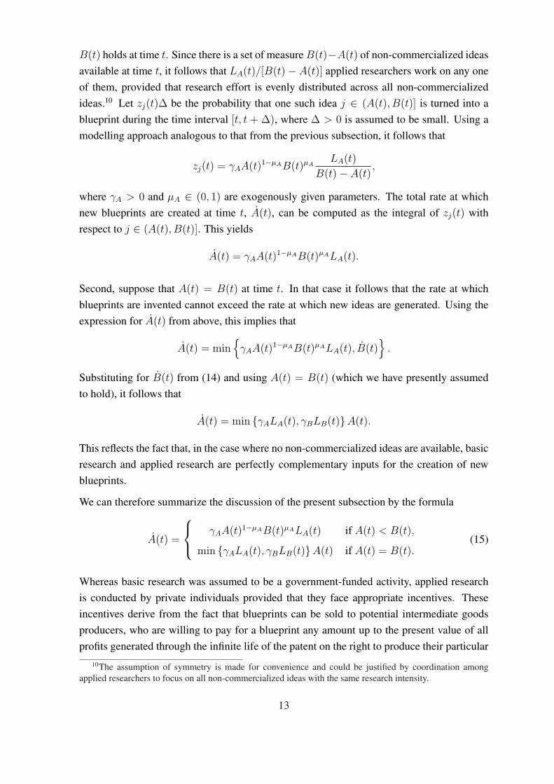
B(t) holds at time t. Since there is a set of measure B(t)−A(t) of non-commercialized ideasavailable at time t, it follows that LA(t)/[B(t)− A(t)] applied researchers work on any oneof them, provided that research effort is evenly distributed across all non-commercializedideas.10 Let zj(t)∆ be the probability that one such idea j ∈ (A(t), B(t)] is turned into ablueprint during the time interval [t, t + ∆), where ∆ > 0 is assumed to be small. Using amodelling approach analogous to that from the previous subsection, it follows that

zj(t) = γAA(t)1−µAB(t)µALA(t)

B(t)− A(t),

where γA > 0 and µA ∈ (0, 1) are exogenously given parameters. The total rate at whichnew blueprints are created at time t, A(t), can be computed as the integral of zj(t) withrespect to j ∈ (A(t), B(t)]. This yields

A(t) = γAA(t)1−µAB(t)µALA(t).

Second, suppose that A(t) = B(t) at time t. In that case it follows that the rate at whichblueprints are invented cannot exceed the rate at which new ideas are generated. Using theexpression for A(t) from above, this implies that

A(t) = min{

γAA(t)1−µAB(t)µALA(t), B(t)}

.

Substituting for B(t) from (14) and using A(t) = B(t) (which we have presently assumedto hold), it follows that

A(t) = min {γALA(t), γBLB(t)}A(t).

This reflects the fact that, in the case where no non-commercialized ideas are available, basicresearch and applied research are perfectly complementary inputs for the creation of newblueprints.

We can therefore summarize the discussion of the present subsection by the formula

A(t) =

γAA(t)1−µAB(t)µALA(t) if A(t) < B(t),

min {γALA(t), γBLB(t)}A(t) if A(t) = B(t).(15)

Whereas basic research was assumed to be a government-funded activity, applied researchis conducted by private individuals provided that they face appropriate incentives. Theseincentives derive from the fact that blueprints can be sold to potential intermediate goodsproducers, who are willing to pay for a blueprint any amount up to the present value of allprofits generated through the infinite life of the patent on the right to produce their particular

10The assumption of symmetry is made for convenience and could be justified by coordination amongapplied researchers to focus on all non-commercialized ideas with the same research intensity.

13

intermediate good. The price at which a new patent can be sold at time t is therefore givenby V (t) as defined in equation (12). The probability to earn this price for any given appliedresearcher in the time interval [t, t+∆) is approximately equal to A(t)∆/LA(t). Combiningthis with equation (15) we see that the expected rate of return to one unit of time spent atinstant t on applied research is equal to

wA(t) =

γAA(t)1−µAB(t)µAV (t) if A(t) < B(t),

min {γA, γB[LB(t)/LA(t)]}A(t)V (t) if A(t) = B(t).(16)

3.6 Government

The government uses two policy instruments expressed by two time paths. First, it employsLB(t) researchers at time t in basic research. Second, research activities are subsidized atthe rate σ(t). We denote the corresponding policy scheme by P = {LB(t), σ(t)}.

Employing LB(t) units of labor in the basic research sector causes a net cost of w(t)LB(t)

to the government, where w(t) is the net real wage introduced in Subsection 3.1. This num-ber already takes into account labor tax received from and research subsidies paid to basicresearchers. The research subsidies paid to applied researchers amount to σ(t)wA(t)LA(t).The sum of these two numbers is total government expenditure which is financed through thetaxation of labor income at the rate τ(t).11 We assume that the government is required to havea balanced budget at all times, which implies that the tax rate τ(t) is uniquely determined bythe budget constraint

w(t)LB(t) + σ(t)wA(t)LA(t) = τ(t)wA(t)LA(t) + τ(t)w(t)[LX(t) + LY (t)]. (17)

The policy scheme P is feasible if LB(t) ∈ [0, L), σ(t) ≥ 0, and τ(t) ∈ [0, 1) hold for all t.

3.7 Market clearing

Having described the behavior of all agents in the economy, let us now turn to market clear-ing. Market clearing on intermediate goods markets has already been taken into account bysubstituting the inverse demand functions into the profit maximization problems of interme-diate goods producers. This leaves us with the markets for labor, assets, and final output.12

The labor market clearing condition is

LA(t) + LB(t) + LX(t) + LY (t) = L. (18)

11As labor supply is inelastic, this is equivalent to imposing a lump-sum tax.12According to Walras’ law, one of the market clearing conditions is redundant.

14

Moreover, there is also a no-arbitrage condition regarding the different possible uses of labor:all those uses that are actually applied must earn the same net real wage w(t). Since per-capita consumption must be positive for all t in every equilibrium, the same must be true foroutput. This, in turn, implies that both LX(t) and LY (t) must be strictly positive at all times.The no-arbitrage condition is therefore

w(t) = [1− τ(t)]w(t) ≥ [1− τ(t) + σ(t)]wA(t) with equality if LA(t) > 0. (19)

Asset market clearing requires that aggregate wealth of the household sector at time t is equalto the total value of all intermediate goods producing firms, i.e.,

a(t) = A(t)V (t)/L (20)

with V (t) given in (12). The market for final output is in equilibrium if

c(t) = Y (t)/L, (21)

because the only demand for final output is the consumption demand of the households.

4 Equilibrium

We are now ready to define an equilibrium of the model. For that purpose and for the re-mainder of the paper we assume that the initial values for blueprints and ideas, A0 and B0,respectively, are given and satisfy 0 < A0 ≤ B0.

Definition 1An equilibrium associated with the initial values A0 and B0 and the policy scheme P =

{LB(t), σ(t)} is a set of time paths E = {Y (t), x(t), A(t), B(t), LA(t), LX(t), LY (t), c(t),r(t), w(t), w(t), wA(t), a(t), π(t), V (t), τ(t)} such that(i) the optimality and market clearing conditions (2), (4)-(6), (9), (11)-(21) hold for all t;(ii) the boundary conditions A(0) = A0, B(0) = B0 are satisfied and (3) holds as an equality;(iii) consumption is strictly positive at all times, i.e., c(t) > 0 for all t;(iv) the tax rate is feasible, i.e., 0 ≤ τ(t) < 1 holds for all t.

The reason why we include the requirement that consumption is strictly positive at all timesis that we want to rule out the trivial equilibrium in which neither final output nor any inter-mediate goods are produced and, hence, consumption, profits, income, and wealth are zeroat all times. Note that the condition c(t) > 0 implies immediately that Y (t) > 0 (becauseof (21)), which in turn implies A(t) > 0, x(t) > 0, and LY (t) > 0 (because of (5)). Hence,also w(t) > 0, LX(t) > 0, π(t) > 0, and V (t) > 0 must hold in equilibrium (because ofequations (6), (13), (11), and (12), respectively).

15

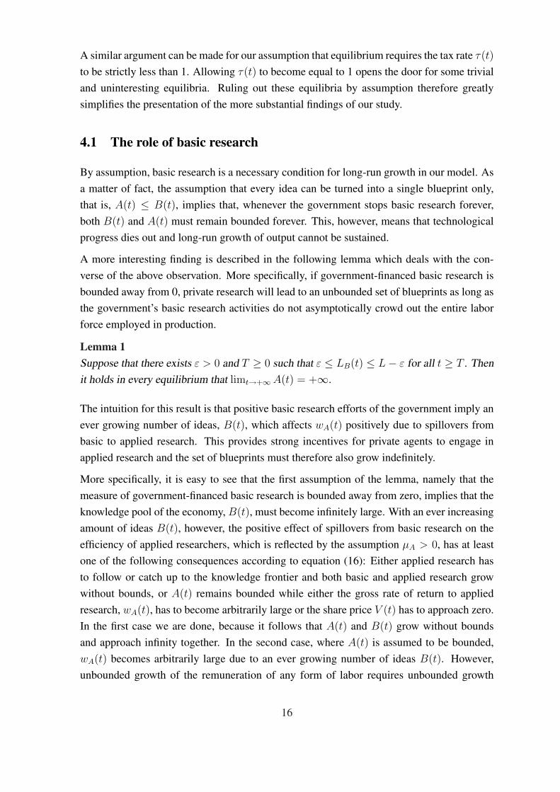
A similar argument can be made for our assumption that equilibrium requires the tax rate τ(t)

to be strictly less than 1. Allowing τ(t) to become equal to 1 opens the door for some trivialand uninteresting equilibria. Ruling out these equilibria by assumption therefore greatlysimplifies the presentation of the more substantial findings of our study.

4.1 The role of basic research

By assumption, basic research is a necessary condition for long-run growth in our model. Asa matter of fact, the assumption that every idea can be turned into a single blueprint only,that is, A(t) ≤ B(t), implies that, whenever the government stops basic research forever,both B(t) and A(t) must remain bounded forever. This, however, means that technologicalprogress dies out and long-run growth of output cannot be sustained.

A more interesting finding is described in the following lemma which deals with the con-verse of the above observation. More specifically, if government-financed basic research isbounded away from 0, private research will lead to an unbounded set of blueprints as long asthe government’s basic research activities do not asymptotically crowd out the entire laborforce employed in production.

Lemma 1Suppose that there exists ε > 0 and T ≥ 0 such that ε ≤ LB(t) ≤ L− ε for all t ≥ T . Thenit holds in every equilibrium that limt→+∞ A(t) = +∞.

The intuition for this result is that positive basic research efforts of the government imply anever growing number of ideas, B(t), which affects wA(t) positively due to spillovers frombasic to applied research. This provides strong incentives for private agents to engage inapplied research and the set of blueprints must therefore also grow indefinitely.

More specifically, it is easy to see that the first assumption of the lemma, namely that themeasure of government-financed basic research is bounded away from zero, implies that theknowledge pool of the economy, B(t), must become infinitely large. With an ever increasingamount of ideas B(t), however, the positive effect of spillovers from basic research on theefficiency of applied researchers, which is reflected by the assumption µA > 0, has at leastone of the following consequences according to equation (16): Either applied research hasto follow or catch up to the knowledge frontier and both basic and applied research growwithout bounds, or A(t) remains bounded while either the gross rate of return to appliedresearch, wA(t), has to become arbitrarily large or the share price V (t) has to approach zero.In the first case we are done, because it follows that A(t) and B(t) grow without boundsand approach infinity together. In the second case, where A(t) is assumed to be bounded,wA(t) becomes arbitrarily large due to an ever growing number of ideas B(t). However,unbounded growth of the remuneration of any form of labor requires unbounded growth

16

of final output which is only possible if the set of blueprints and thus of new intermediategoods grows indefinitely. Hence, it follows, that A(t) also needs to be unbounded, which isa contradiction. The remaining case of A(t) assumed to be bounded and V (t) approachingzero can be shown to occur only if final output and, hence, also the labor inputs LX(t) andLY (t) approach zero. Together with (18) and the second assumption of the lemma, namelythat basic research employment LB(t) is bounded away from L, this would imply that LA(t)

remains bounded away from zero, which, again, leads to unbounded growth of A(t), whichis again a contradiction.

4.2 Balanced growth paths

In this subsection, we focus on time-invariant policy schemes P = {LB, σ}, where bothLB ∈ [0, L) and σ ≥ 0 are constants. We examine the existence of balanced growth paths(BGPs), that is, equilibria along which all endogenous variables grow at constant rates.

Along a BGP equilibrium the labor shares LA(t), LX(t), LY (t) as well as the tax rate τ(t)

must be constant over time. We will therefore omit the time argument from these func-tions. Analogously, along a BGP equilibrium, the growth rate of per-capita consumptionis constant. From the Euler equation (4) it follows therefore that the real interest rate isalso constant, and we can simply write r instead of r(t). Finally, we shall denote for anystrictly positive and differentiable function v by gv(t) its growth rate at time t defined bygv(t) ≡ v(t)/v(t).

Lemma 2Along every BGP equilibrium A(t) and B(t) must grow at the same rate, that is, the equationgA(t) = gB(t) holds for all t ≥ 0.

The above result is a consequence of the existence of spillovers between the two researchsectors as reflected by the assumptions µA > 0 and µB > 0. Research activities in one sectorshape research activities in the other sector, and vice versa.

Let us henceforth denote the common growth rate of A(t) and B(t) by g. For the followinganalysis it will be convenient to define the functions D(g), F (g, LB, σ), and H(LB, σ) by

D(g) ≡ (1− α + α2)ρ + g,

F (g, LB, σ) ≡ α(1− α)γA[D(g)(L− LB) + (1− α + α2)(g + ρ)σL]/D(g)2,

H(LB, σ) ≡ F (γBLB, LB, σ).

We have the following technical lemma.

Lemma 3(a) The function D(g) is continuous, strictly positive, and strictly increasing for all g ∈[0, +∞).

17

(b) The function F (g, LB, σ) is continuous, strictly positive, strictly decreasing with respectto g ∈ [0, +∞) and LB ∈ [0, L), and strictly increasing with respect to σ ∈ [0, +∞).(c) The function H(LB, σ) is continuous, strictly positive, strictly decreasing with respect toLB ∈ [0, L), and strictly increasing with respect to σ ∈ [0, +∞).

From the properties of F (g, LB, σ) and H(LB, σ) stated in Lemma 3 the following resultsare obvious. First, whenever LB ∈ [0, L) and σ ∈ [0, +∞), then there exists a uniquenumber g > 0 such that13

F (g, LB, σ) = [g/(γBLB)]µA/µB . (22)

Second, the equation H(LB, σ) = 1 has a unique solution on the interval LB ∈ [0, L) if andonly if H(0, σ) ≥ 1 > H(L, σ). In that case let us denote this solution by LB. We define

LB =

0 if H(0, σ) < 1,

LB if H(0, σ) ≥ 1 > H(L, σ),

L if H(L, σ) ≥ 1.

We are now ready to state the main result of this section. It presents both a necessary and asufficient condition for a BGP equilibrium with growth rate g to exist.

Theorem 1(a) If g is the common growth rate of the variables A(t) and B(t) in a BGP equilibriumcorresponding to the constant policy scheme P = {LB, σ}, then it follows that

g =

γBLB if LB ≤ LB,

g if LB > LB,(23)

and

A(t)/B(t) =

1 if 0 < LB ≤ LB,

[g/(γBLB)]1/µB < 1 if LB > LB.(24)

Moreover, final output and consumption grow at the common rate gY = gc = (1 − α)g andthe interest rate is given by r = (1− α)g + ρ.(b) Suppose that g satisfies (23) and that

D(g)(L− LB) > α(1− α)gσL. (25)

Then there exists a BGP equilibrium corresponding to the policy scheme P = {LB, σ} alongwhich the variables A(t) and B(t) grow at the rate g.

13This is obvious because the left-hand side of (22) is strictly positive and decreases continuously as gmoves from 0 to +∞, whereas the right-hand side increases continuously from 0 to +∞.

18

4.3 Discussion

In this subsection we provide a detailed discussion of Theorem 1.

The impact of LB

Part (a) of the theorem states conditions which the economic growth rate g and the ratiobetween blueprints and ideas A(t)/B(t) must necessarily satisfy in equilibrium. These con-ditions (23)-(24) depend crucially on the threshold level LB ∈ [0, L].

Let us first consider the case in which the measure of basic researchers LB employed by thegovernment does not exceed LB. In this situation we can see that applied researchers instan-taneously commercialize any available basic research idea by turning it into a commercialblueprint. This is reflected by the result that A(t)/B(t) = 1 holds permanently. The reasonis that, in this case, too little basic research is performed to permanently push the knowledgefrontier of the economy ahead of applied research and, hence, applied researchers can com-pletely exhaust the pool of ideas. According to (23), this implies that the overall growth rateg is only determined by the size of the publicly funded basic research sector, LB, as well asby the productivity in the basic research sector, γB. Both of these variables have a strictlypositive impact. In other words, in case of LB ≤ LB, basic research is the sole engine oflong-run growth.

As mentioned above, in the case where LB ≤ LB, applied research always operates atthe knowledge frontier. This implies in particular that applied research and, hence, overalleconomic growth has to cease unless positive basic research efforts permanently increase theknowledge pool of the economy. This also explains why research subsidies σ do not haveany effect on the growth rate g whenever LB ≤ LB.14 As applied research already operatesat the knowledge frontier, granting subsidies in order to stimulate further applied researchwould be ineffective.

In contrast, if LB exceeds the threshold value LB, basic research pushes the knowledgefrontier fast enough such that, at each instant in time, a pool of non-commercialized ideas isavailable that has not yet been turned into blueprints through applied research. According to(24), the ratio of blueprints to ideas, A(t)/B(t), is then strictly smaller than 1 showing thatthe available pool of non-commercialized ideas is never exhausted. In fact, the measure ofnon-commercialized ideas grows without bounds. The growth rate g = g is given by (22)and can be shown to lie between γALA and γBLB. Thus, in the case of LB > LB, long-rungrowth is shaped by both basic and applied research together.

The intuitive reason for this result is that, while applied research stimulates growth by com-mercializing basic research, the potential of generating growth is upward bounded by therate at which new ideas are created, i.e., by how fast the knowledge frontier of the economy

14Note, however, that the threshold level LB itself depends on the size of σ.

19

is pushed ahead through basic research and how this impacts on the speed of commercializa-tion.

We would like to emphasize that, while g is strictly increasing with respect to LB ∈ [0, LB],the relation between g = g and LB can become more complicated for LB > LB. This isshown by the following example.

EXAMPLE: Suppose that

σ = 0 and L >(1− α + α2)ρ

α(1− α)γA

. (26)

Simple algebra shows that these assumptions imply

LB =α(1− α)γAL− (1− α + α2)ρ

α(1− α)γA + γB

> 0. (27)

Now assume in addition that µA = µB. In that case we can solve equation (22) to obtain

g = −(1− α + α2)ρ

2+

√(1− α + α2)2ρ2

4+ γAγBα(1− α)LB(L− LB).

Combining this result with (23) we see that the equilibrium growth rate increases linearlywith LB on the interval [0, LB], whereas it is described by a unimodal function of LB onthe interval [LB, L). It follows in particular that g is decreasing with respect to LB on[max{LB, L/2}, L), whereas it is increasing on [LB, L/2] provided this interval is non-empty. The latter case illustrates that the growth rate may depend positively on the publicbasic research input LB even if the pool of non-commercialized ideas remains permanentlynon-empty. ¤

The example illustrates that an increase of LB has two opposite effects on applied research.First, the associated increase of B(t) triggered by a high amount of basic research affectsapplied research positively through knowledge spillover. Second, an increase of LB alsohas a negative influence on applied research because it ties up labor that otherwise couldbe used for other purposes. As long as the positive spillover effect dominates, an increaseof LB induces higher growth, and both gB and gA are increasing with respect to LB. Assoon as LB exceeds a critical value, however, the negative effect of reducing labor supply forapplied research and production dominates and gA becomes decreasing with respect to LB.Any decline of gA is associated with a corresponding decrease of gB as spillovers to basicresearch diminish. That is, an increase of basic research is not only detrimental to overallgrowth, but also to the generation of new ideas.

The impact of research subsidies

We have already noted that research subsidies have no impact on growth for LB ≤ LB be-cause in that situation applied research operates at the knowledge frontier. For LB > LB,

20

however, equations (22) and (23) imply that the level of research subsidies, σ, has a strictlypositive impact on growth. The reason is quite obvious as increasing the research subsidieslowers the relative cost of performing applied research and thus induces more labor to beemployed in applied research. Furthermore, the threshold value LB itself is an increasingfunction of the research subsidy σ. The reason is that granting higher research subsidies in-creases the incentives to work in the applied research sector, thereby shifting the labor supplytowards the applied research sector, and consequently accelerates growth of A(t). Therefore,for any given growth rate of B(t), a higher research subsidy makes it more likely that appliedresearch catches up to the knowledge frontier of the economy and the long-run ratio betweenblueprints and ideas, A(t)/B(t), increases. In other words, with a higher subsidization of re-search, the speed of commercialization of ideas accelerates and the knowledge frontier morelikely becomes a binding constraint for applied research.

Feasibility and boundary conditions

Condition (25) in part (b) of Theorem 1 ensures that the BGP equilibrium is feasible in thesense that it fulfils the requirement τ ∈ [0, 1); see part (iv) of Definition 1. It is obvious thatτ will be equal to zero if and only if both LB = 0 and σ = 0, because the only expendituresof the government are its outlays on basic research and subsidies. On the other hand, it ispossible that the employment of a large number of basic researchers and/or the payment ofhigh research subsidies would require the government to set τ ≥ 1, which is not feasible. Torule out this possibility, (25) imposes a joint restriction on the policy parameters LB and σ

that ensures that both government activities can be financed by a labor tax at rate τ < 1.

We finally note that the threshold value LB itself could be equal to 0. In such circumstancesall positive levels of basic research input lead to a situation where the measure of blueprintsis strictly smaller than the measure of ideas (A(t) < B(t)). Whether LB = 0 or not dependson whether H(0, σ) ≤ 1 or not. From the definition of H(LB, σ) we can see in particularthat LB = 0 holds if and only if

α(1− α)γAL(1 + σ)

(1− α + α2)ρ≤ 1. (28)

5 One-directional spillovers

So far we have assumed that spillovers are present both from basic to applied research andvice versa. Formally, this is reflected by the assumptions µA > 0 and µB > 0, which wehave explicitly used in the proofs of Lemmas 1 and 2 and implicitly in the proof of Theorem1. In this section we discuss the two special cases in which non-negligible spillovers occuronly in one of these directions, that is, we analyze what happens in the limits when either µA

or µB approaches 0.

21

To this end note that none of the functions D(g), F (g, LB, σ), and H(LB, σ) depends on theparameters µA and µB. This implies in particular that the threshold value LB is independentof these parameters. However, as is clear from equation (22), the relative size of the spilloverparameters µA and µB is a crucial determinant of g.

5.1 Only upward spillovers

Let us start with the case where µA > 0 is fixed and µB approaches 0. In this limit, the effectof the measure of blueprints on the productivity of basic researchers becomes negligible,whereas the measure of existing ideas has a strictly positive influence on the productivityof applied researchers. Hence, there is upward spillover from basic to applied research, butonly negligible downward spillover from applied to basic research. As µB converges to 0,the right-hand side of equation (22) approaches 0 whenever g < γBLB and it approaches+∞ if g > γBLB. This proves immediately that g, the unique solution of equation (22),converges to the value γBLB as µB approaches 0. Using this result together with condition(23) we can conclude that in the case where µB ≈ 0, the equilibrium growth rate satisfiesg ≈ γBLB for all settings of LB and σ. We formally state this finding as the first result inthe following lemma.

Lemma 4In the limit, when µB approaches zero, the equilibrium growth rate is given by g = γBLB.Furthermore, it holds that

limµB→0

A(t)/B(t) =

1 if 0 < LB ≤ LB,

H(LB, σ)1/µA < 1 if LB > LB.

This implies that, in the absence of significant downward spillovers from applied to basicresearch, long-run growth of the economy only depends on the amount of basic researchconducted by the government, LB, as well as on the productivity parameter γB. In particular,it follows that the research subsidy σ has no growth effect when only upward spillovers arepresent. In the case where LB ≤ LB, this finding is obvious and just repeats what we havealready established for the model with two-way spillovers in section 4: if applied researchoperates at the knowledge frontier, overall growth is restricted by the size and productivityof the basic research sector and cannot be further increased by research subsidies. Surpris-ingly, however, the same result holds here also when LB > LB, in which case the set ofnon-commercialized ideas is never exhausted. To understand why, first note that (14) andµB arbitrarily small together imply that the evolution of the knowledge frontier dependssolely on the current location of this frontier, on the productivity parameter γB, and on theamount of labor employed in basic research: the growth rate is gB = γBLB. By subsidizingresearchers at a higher rate σ, the government can make the gap between the set of com-mercialized blueprints and basic research ideas smaller, but, since the measure of blueprints

22

does not feed back onto the productivity of basic researchers, this leaves the growth rate gB

unaffected. Thus, in the case of one-directional upward spillovers, long-run growth can onlybe stimulated through basic research.

5.2 Only downward spillovers

We now turn to the case of negligible upward spillovers, i.e., the case where µB > 0 is givenand µA approaches 0. In this limiting case the right-hand side of equation (22) converges to1 whenever g > 0. This implies that in the limit it must hold that

g =

¯g if F (0, LB, σ) > 1,

0 if F (0, LB, σ) ≤ 1,(29)

where ¯g is uniquely determined by the condition F (g, LB, σ) = 1. Combining this resultwith (23) we obtain the following lemma in which ¯LB is defined by

¯LB = (1 + σ)L− (1− α + α2)ρ

α(1− α)γA

.

Lemma 5(a) The condition ¯LB ≤ 0 holds if and only if LB = 0. Moreover, whenever LB > 0 then itfollows that LB < ¯LB.(b) Suppose that µB > 0 is fixed. In the limit as µA approaches 0, the equilibrium growthrate is given by

g =

γBLB if LB ≤ LB,

¯g if LB < LB ≤ ¯LB,

0 if LB > ¯LB.

Lemma 5 indicates that there are three different facets of growth. First, if the actual amountof basic researchers LB does not exceed the threshold LB, basic research alone shapes long-run growth. In this facet the research subsidy σ has no growth effects, because appliedresearchers already operate at the knowledge frontier. Second, if LB exceeds the thresholdLB, but remains beneath ¯LB, then growth is shaped both by basic and applied research.From the definition of ¯g one can see that ¯g is increasing with respect to σ and decreasingwith respect to LB. It follows therefore from Lemma 5 that the growth rate g is maximal ifLB = LB. Any expansion of the basic research sector beyond the threshold value LB wouldbe detrimental to growth. That is, along the interval [LB, ¯LB] growth decreases until it isabout to cease entirely in case LB approaches ¯LB. Third, if LB exceeds ¯LB the equilibriumgrowth is equal to zero. These results are further illustrated by the following example.

23

EXAMPLE: As in the previous example assume that (26) holds. In addition to (27), thisimplies that

¯LB = L− (1− α + α2)ρ

α(1− α)γA

> LB,

¯g = α(1− α)γA(L− LB)− (1− α + α2)ρ.

Using these expressions in Lemma 5 one sees that the equilibrium growth rate g in the caseof negligible upward spillovers is a continuous and piecewise linear function of LB thatincreases on the interval [0, LB], decreases on [LB, ¯LB], and is constant and equal to 0 on[ ¯LB, L). ¤

5.3 Summary

The results for one-directional spillovers discussed above provide valuable information aboutthe hierarchy and interdependence of basic and applied research and about their joint effecton growth. More specifically, we have seen that in the absence of significant downwardspillovers from applied to basic research more publicly funded basic research always trans-lates into faster growth. On the other hand, in the absence of significant upward spilloversfrom basic to applied research, growth depends positively on the public basic research inputonly as long as applied researchers find it optimal to completely exhaust the available knowl-edge base of the economy at each point in time. The general case covered by Theorem 1 canbe considered as a mixture of the two special cases discussed in the present section.

6 An illustration

6.1 Replication of the US growth pattern

In this section we provide an illustrative example of above model. We replicate the USinnovation pattern and growth rate.

Parameter Choices

For this purpose, we consider the following parameter values. For the elasticity of finaloutput with respect to intermediate goods, α, we assume that new intermediates enter finalgoods production as new varieties of capital goods. To obtain a plausible value for α withinour endogenous growth framework, we borrow from the existing empirical growth literature,where the share of capital in final goods production has been subject to various empiricalestimates of the neoclassical growth model. Thereby, the quantitative extent of α cruciallydepends on the underlying concept of capital that is taken into account. More specifically, the

24

conventional share of physical capital is α = 1/3 (see, for example, Jones, 2002), which mayeven be as low as 0.1 for an open economy (Barro et al., 1995). However, when assumingthat the underlying concept of capital also includes human capital, the conventional capitalshare appears too narrow and one should rather focus on a broader concept of capital (see,for example, Barro and Sala-i-Martin, 1992, and Mankiw et al., 1992). Thus, assuming thathuman capital is embodied entirely in new varieties of intermediate capital goods wouldimply a value of up to α = 0.8 (Barro and Sala-i-Martin, 1992). As this last case appearsto correspond closest to our model, we set α = 0.8. Furthermore, we follow Barro andSala-i-Martin (1992) and set the time-preference rate to ρ = 0.05. Finally, we set L = 1.

Data on basic and applied research employment are usually harder to obtain. Accordingto National Science Board (2008), scientists and engineers made up about 4.2 percent ofthe total US workforce in 2006, while figures from 2003 suggest that out of these about 59

percent were employed by industry, while the remaining 41 percent were mainly affiliatedwith government and university institutions. This suggests that LB = 0.017. In addition, weassume an equal intensity of spillovers from basic to applied research and vice versa, andset our spillover parameters to µA = µB = 0.5, while our research productivity parametersγA and γB are set to γA = γB = 5.3. Finally, we set research subsidies σ equal to zero andassume an initial amount of basic research ideas, B(0), equal to 10.

Simulations

Given these parameter settings, our simulations yield that g = 0.09. According to Theorem1 this implies that the growth rate of per capita GDP is gY = g(1−α) = 0.018. This is equalto the average long-run growth of per capita GDP in the US per year which has been foundto be about 1.8 percent (see for example, Jones, 2002, or Barro and Sala-i-Martin, 2004).

Furthermore, the share of applied researchers in the total labor force is LA = 0.107. Whilethe growth rate corresponds exactly to the average annual, long-run US growth rate statedabove, the share of applied research employment LA at first glance appears quite high ascompared to the suggested value of LA = 0.025 by the data of the National Science Board(2008). However, the official data about research employment are significantly downward-biased as they merely focus on scientists and engineers and also require those to have acollege degree, whereby a considerable amount of researchers is not captured by these data(Jones, 2002). In that regard, a share of applied research as high as LA = 0.107 appearsto be not implausible. Our simulations also suggest that the US innovation and growthsystem operates at the knowledge frontier, that is A(t)/B(t) = 1. Therefore, growth isonly shaped by basic research LB as well as the research productivity parameter γB, whilethe remaining parameters have at most an impact on applied research employment LA andon output. Finally, we note that employing LB = 0.017 basic researchers, while granting noresearch subsidies σ corresponds to a feasible policy scheme in the sense that condition (25)of Theorem 1 is fulfilled

25

6.2 Policy changes

It is useful to evaluate how policy changes would impact on growth in the simulated econ-omy. In particular, suppose we vary LB ∈ (0, 0.2] and γB = (0, 10] in the above system.Figure 1 shows the impact of variations in the amount of basic research LB while holdingfixed all other parameters of the model. As shown in the upper graph, along the knowledgefrontier the growth rate g increases linearly with the amount of basic research LB. A con-tinuous increase of basic research eventually results in LB exceeding the threshold amountLB. From there on, basic research continues to have a positive, albeit diminishing effect onlong-run growth. For ever larger values of LB the growth rate would start to decline until itreaches zero when all labor would be employed in basic research. The amount of appliedresearch LA first increases with basic research LB as the associated increase in the speedof creating novel ideas also increases incentives for applied research via spillovers. Thisincrease of LA reverses, however, as soon as increasing levels of basic research can only beachieved by withdrawing labor from applied research. As can be seen in the lower graph,low levels of basic research allow the economy to operate at the knowledge frontier. As soonas LB achieves the threshold value LB, however, further increases of basic research triggeran increasing distance to the knowledge frontier. We note that the ratio of blueprints to ideas,A(t)/B(t), converges to zero when LB would converge to 1.

0 0.02 0.04 0.06 0.08 0.1 0.12 0.14 0.16 0.18 0.20

0.2

0.4

0.6

0.8

1

LB

LA

g

0 0.02 0.04 0.06 0.08 0.1 0.12 0.14 0.16 0.18 0.2

0.65

0.7

0.75

0.8

0.85

0.9

0.95

1

LB

A/B

Figure 1: The impact of basic research LB

Figure 2 shows the effect of varying the research productivity parameter γB while holding allother model parameters fixed. As the upper graph shows, γB has a strictly positive impact ongrowth. A higher γB also exerts a positive, but decreasing impact on applied research, LA, ashigher productivity of basic research, which leads to a faster growing number of ideas, also

26

increases incentives to engage in applied research. Furthermore, as the threshold value LB

is a function of γB, a further continuous increase of γB at some stage induces basic researchto be productive enough such that the number of ideas will evolve faster than the number ofblueprints, and applied research falls short of basic research. That is, for sufficiently highγB, applied research would no longer operate at the knowledge frontier of the economy.

0 1 2 3 4 5 6 7 8 9 100

0.05

0.1

0.15

0.2

γB

LA

g

0 1 2 3 4 5 6 7 8 9 100

0.5

1

1.5

2

γB

A/B

Figure 2: The impact of basic research productivity γB

7 Conclusion

We have developed a simple model that combines the hierarchy of basic and applied researchas well as their interdependence with an expanding variety growth framework. Numerousissues deserve further scrutiny. In particular, a normative analysis of our model could be usedto develop guidelines for socially optimal policies regarding the amount of basic research andresearch subsidies.

27

References

[1] Aagaard, Lars and Rossi, John J. (2007): “RNAi therapeutics: Principles, prospectsand challenges,” Advanced Drug Delivery Reviews, 59(2-3), 75-86

[2] Acs, Zoltan J., Audretsch, David B., and Feldman, Maryann P. (1992): “Real Effectsof Academic Research: Comment,” American Economic Review, 82(1), 363-367

[3] — (1994): “R&D Spillovers and Recipient Firm Size,” Review of Economics andStatistics, 76(2), 336-340

[4] Adams, James D. (1990): “Fundamental Stocks of Knowledge and ProductivityGrowth,” Journal of Political Economy, 98(4), 673-702

[5] Adams, James D., Chiang, Eric P., and Starkey, Katara (2001): “Industry-UniversityCooperative Research Centers,” Journal of Technology Transfer, 26(1-2), 73-86

[6] Agrawal, Ajay and Henderson, Rebecca (2002): “Putting Patents in Context: Explor-ing Knowledge Transfer from MIT,” Management Science, 48(1), 44-60

[7] Ahmadian, Afshin, Ehn, Maria, and Hober, Sophia (2006): “Pyrosequencing: History,Biochemistry and Future,” Clinica Chimica Acta, 363(1-2), 83-94

[8] Ajdari, Armand (2007): “Pierre-Gilles de Gennes (1932-2007),” Science, 317, 466

[9] Anderson, John D. Jr. (2005): “Ludwig Prandtl’s Boundary Layer,” Physics Today,58(12), 42-48

[10] Assmus, Alexi (1995): “Early History of X Rays,” Beam Line, 25(2), 10-24

[11] Bania, Neil, Eberts, Randall W., and Fogarty, Michael S. (1993): “Universities and theStartup of New Companies: Can We Generalize from Route 128 and Silicon Valley?,”Review of Economics and Statistics, 75(4), 761-766

[12] Barnes, Susan B., (1997): “Douglas Carl Engelbart: Developing the Underlying Con-cepts for Contemporary Computing,” IEEE Annals of the History of Computing,19(3), 16-26

[13] Barro, Robert J. and Sala-i-Martin, Xavier (1992): “Convergence.” Journal of PoliticalEconomy, 100(2), 223-251

[14] — (2004): Economic Growth, 2nd edition, MIT Press

[15] Barro, Robert J., Mankiw, N. Gregory, and Sala-i-Martin, Xavier (1995): “CapitalMobility in Neoclassical Models of Growth,” American Economic Review, 85(1),103-115

28

[16] Blumberg, Baruch S. (1997): “Hepatitis B Virus, the Vaccine, and the Control of Pri-mary Cancer of the Liver,” Proceedings of the National Academy of Sciences, 94(14),7121-7125

[17] Brochard-Wyart, Francoise (2007): “Obituary: Pierre-Gilles de Gennes (1932-2007)- Pioneer of Soft-Matter Physics,” Nature, 448(7150), 149

[18] Bunch, T. Jared and Day, John D. (2008): “The Diagnostic Evolution of the CardiacImplantable Electronic Device: The Implantable Monitor of Ischemia,” Journal ofCardiovascular Electrophysiology, 19(3), 282-284

[19] Cohen, Stanley N., Chang, Annie C. Y., Boyer, Herbert W., and Helling, Robert B.(1973): “Construction of Biologically Functional Bacterial Plasmids In Vitro,” Pro-ceedings of the National Academy of Sciences, 70(11), 3240-3244

[20] Cohen, Wesley M., Nelson, Richard R., and Walsh, John P. (2002): “Links and Im-pacts: The Influence of Public Research on Industrial R&D,” Management Science,48(1), 1-23

[21] Colyvas, Jeannette, Crow, Michael, Gelijns, Annetine, Mazzoleni, Roberto, Nelson,Richard R., Rosenberg, Nathan, and Sampat, Bhaven N. (2002): “How Do UniversityInventions Get into Practice ?,” Management Science, 48(1), 61-72

[22] Donald, Stewart M. (2007): “Sir John Charnley (1911-1982): Inspiration to FutureGenerations of Orthopaedic Surgeons,” Scottish Medical Journal, 52(2), 43-46

[23] Funk, Mark (2002): “Basic Research and International Spillovers,” International Re-view of Applied Economics, 16(2), 217-226

[24] Ellington, Charles P., van den Berg, Coen, Willmott, Alexander P., and Thomas,Adrian L. R. (1996): “Leading-Edge Vortices in Insect Flight,” Nature, 384(6610),626-630

[25] Elmqvist, Rune, Johan, Landegren, Pettersson, Sven Olov, Senning, Ake, andWilliam-Olsson, Goran (1963): “Artificial Pacemaker for Treatment of Adams-StokesSyndrome and Slow Heart Rate,” American Heart Journal, 65(6), 731-748

[26] Fire, Andrew, Xu, SiQun, Montgomery, Mary K., Kostas, Steven A., Driver, SamuelE., and Mello, Craig C. (1998): “Potent and specific genetic interference by double-stranded RNA in Caenorhabditis elegans,” Nature, 391(6669), 806-811

[27] Gancia, Gino and Zilibotti, Fabrizio (2005): “Horizontal Innovation in the Theoryof Growth and Development,” in: Aghion, Philippe and Durlauf, Steven N. (eds.),Handbook of Economic Growth, Elsevier

29

[28] Gelijns, Annetine C. and Rosenberg, Nathan (1999): “Diagnostic Devices: An Analy-sis of Comparative Advantages,” in: Mowery, David C. and Nelson, Richard R. (eds.),Sources of Industrial Leadership - Studies of Seven Industries, Cambridge UniversityPress

[29] Gibbon, John H. Jr (1978): “The Development of the Heart-Lung Apparatus,” Amer-ican Journal of Surgery, 135(5), 608-619

[30] Grossman, Gene M. and Helpman, Elhanan (1991): Innovation and Growth in theGlobal Economy, MIT Press

[31] Henderson, Rebecca, Jaffe, Adam B., and Trajtenberg, Manuel (1998): “Universitiesas a Source of Commercial Technology: A Detailed Analysis of University Patenting,1965-1988,” Review of Economics and Statistics, 80(1), 119-127

[32] Hirschel, Ernst Heinrich, Prem, Horst, and Madelung, Gero (2004): AeronauticalResearch in Germany - from Lilienthal until Today, Springer Verlag

[33] Hopkins, Harold H. and Kapany, Narinder S. (1954): “A Flexible Fibrescope, UsingStatic Scanning,” Nature, 173(4392), 39-41

[34] Hora, Heinrich (2000): Book Review: Charles Townes (1999): How the Laser Hap-pened: Adventures of a Scientist, Laser and Particle Beams, 18(1), 151-152

[35] Jaffe, Adam B. (1989): “Real Effects of Academic Research,” American EconomicReview, 79(5), 957-970

[36] Jensen, Richard and Thursby, Marie (2001): “Proofs and Prototypes for Sale: TheLicensing of University Inventions,” American Economic Review, 91(1), 240-259

[37] Jones, Charles I. (2002): “Sources of U.S. Economic Growth in a World of Ideas,”American Economic Review, 92(1), 220-239

[38] King, Spencer B. III (1996): “Angioplasty From Bench to Bedside to Bench,” Circu-lation, 93(9), 1621-1629

[39] Lauterbur, Paul C. (1973): “Image Formation by Induced Local Interactions: Exam-ples Employing Nuclear Magnetic Resonance,” Nature, 242(5394), 190-191

[40] Leach, Martin O. (2004): “Nobel Prize in Physiology or Medicine 2003 Awarded toPaul Lauterbur and Peter Mansfield for Discoveries Concerning Magnetic ResonanceImaging,” Physics in Medicine and Biology, 49(3), Editorial

30

[41] Leiner, Barry M., Cerf, Vinton G., Clark, David D., Kahn, Robert E., Kleinrock,Leonard, Lynch, Daniel C., Postel, Jon, Roberts, Lawrence G., and Wolff, StephenS. (1997): “The Past and Future History of the Internet,” Communications, 40(2),102-108

[42] Lightman, Alan (2005): The Discoveries: Great Breakthroughs in 20th Century Sci-ence, Pantheon Books, New York

[43] Lynn, John G., Zwemer, Raymund L., Chick, Arthur J., and Miller, August E. (1942):“A New Method for the Generation and Use of Focused Ultrasound in ExperimentalBiology,” Journal of General Physiology, 26(2), 179-193

[44] Mankiw, N. Gregory, Romer, David, and Weil, David N. (1992): “A Contribution tothe Empirics of Economic Growth,” Quarterly Journal of Economics, 107(2), 407-437

[45] Mansfield, Edwin (1991): “Academic Research and Industrial Innovation,” ResearchPolicy, 20(1), 1-12

[46] — (1992): “Academic Research and Industrial innovation: A Further Note,” ResearchPolicy, 21(3), 295-296

[47] — (1995): “Academic Research Underlying Industrial Innovations: Sources, Charac-teristics, and Financing,” Review of Economics and Statistics, 77(1), 55-65

[48] — (1998): “Academic Research and Industrial Innovation: An Update of EmpiricalFindings,” Research Policy, 26(7-8), 773-776

[49] Mansfield, Peter and Grannell, Peter K. (1973): “NMR ’Diffraction’ in Solids?,” Jour-nal of Physics C: Solid State Physics, 6(22), L422

[50] Martin, Ben, Salter, Ammon, Hicks, Diana, Pavitt, Keith, Senker, Jacky, Sharp, Mar-garet, and von Tunzelmann, Nick (1996): The Relationship Between Publicly FundedBasic Research and Economic Performance - A SPRU Review, Science Policy Re-search Unit, University of Sussex, Report prepared for HM Treasury

[51] Maxam, Allan M. and Gilbert, Walter (1977): “A New Method for Sequencing DNA,”Proceedings of the National Academy of Sciences, 74(2), 560-564

[52] Morales, Marıa F. (2004): “Research Policy and Endogenous Growth,” Spanish Eco-nomic Review, 6(3), 179-209

[53] Mowery, David C. and Sampat, Bhaven N. (2005): “Universities in National Innova-tion Systems,” in: Fagerberg, Jan, Mowery, David C., Nelson, Richard R. (eds.), TheOxford Handbook of Innovation, Oxford University Press

31

[54] Myers, Brad A. (1998): “A Brief History of Human-Computer Interaction Technol-ogy,” Interactions, 5(2), 44-54

[55] National Academy of Engineering (2003): The Impact of Academic Research on In-dustrial Performance, National Academies Press

[56] National Science Board (2008): Science and Engineering Indicators 2008

[57] Nelson, Richard R. (1986): “Institutions Supporting Technical Advance in Industry,”American Economic Review - Papers and Proceedings, 76(2), 186-189

[58] — (1993): National Innovation Systems: A Comparative Analysis, Oxford UniversityPress

[59] OECD (2002): Frascati Manual - Proposed Standard Practice for Surveys on Researchand Experimental Development

[60] Owen-Smith, Jason, Riccaboni, Massimo, Pammolli, Fabio, and Powell, Walter W.(2002): “A Comparison of U.S. and European University-Industry Relations in theLife Sciences,” Management Science, 48(1), 24-43

[61] Pan, Zicheng, Sun, Hong, Zhang, Yi, and Chen, Changfeng (2009): “Harder thanDiamond: Superior Indentation Strength of Wurtzite BN and Lonsdaleite,” PhysicalReview Letters, 102(5), 055503(1)-055503(4)

[62] Park, Walter G. (1998): “A Theoretical Model of Government Research and Growth,”Journal of Economic Behavior and Organization, 34(1), 69-85

[63] Perkmann, Markus and Walsh, Kathryn (2008): “Engaging the Scholar: Three Typesof Academic Consulting and Their Impact on Universities and Industry,” ResearchPolicy, 37(10), 1884-1891

[64] Romer, Paul M. (1990): “Endogenous Technological Change,” Journal of PoliticalEconomy, 98(5-2), 71-102

[65] Salter, Ammon J. and Martin, Ben R. (2001): “The Economic Benefits of PubliclyFunded Basic Research: a Critical Review,” Research Policy, 30(3), 509-532

[66] Sanger, Frederick, Nicklen, Steve, and Coulson, Alan R. (1977): “DNA SequencingWith Chain-Terminating Inhibitors,” Proceedings of the National Academy of Sci-ences, 74(12), 5463-5467

[67] Shell, Karl (1966): “Toward a Theory of Inventive Activity and Capital Accumula-tion,” American Economic Review, 56(1/2), 62-68

32

[68] — (1967): “A Model of Inventive Activity and Capital Accumulation,” in: Shell, Karl(ed.), Essays on the Theory of Optimal Economic Growth, MIT Press, Cambridge,Massachusetts

[69] Simoni, Robert D., Hill, Robert L., and Vaughan, Martha (2002): “The Discoveryof Insulin: the Work of Frederick Banting and Charles Best,” Journal of BiologicalChemistry, 277(26), 31-32

[70] Sittig, Dean F., Ash, Joan S., and Ledley, Robert S. (2006): “The Story Behind theDevelopment of the First Whole-Body Computerized Tomography Scanner as Told byRobert S. Ledley,” Journal of the American Medical Informatics Association, 13(5),465-469

[71] Sluckin, Timothy J. (2000): “The Liquid Crystal Phases: Physics and Technology,”Contemporary Physics, 41(1), 37-56

[72] Sluckin, Timothy J., Dunmur, David A., and Stegemeyer, Horst (2004): Crystals thatFlow - Classic Papers from the History of Liquid Crystals, Taylor & Francis, London

[73] Toon, John (2001): “Flying On Mars,” Research Horizons, 19(1), 19-23

[74] Vacanti, Charles A. (2006): “History of Tissue Engineering and A Glimpse Into ItsFuture,” Tissue Engineering, 12(5), 1137-1142

[75] van Heel, Abraham C. S. (1954): “A New Method of Transporting Optical Imageswithout Aberrations,” Nature, 173(4392), 39

[76] von Hippel, Eric (1988): The Sources of Innovation, Oxford University Press

[77] Zellner, Christian (2003): “ The Economic Effects of Basic Research: Evidence forEmbodied Knowledge Transfer via Scientists’ Migration,” Research Policy, 32(10),1881-1895

[78] Zucker, Lynne G., Darby, Michael R., and Brewer, Marilynn B. (1998): “IntellectualHuman Capital and the Birth of U.S. Biotechnology Enterprises,” American EconomicReview, 88(1), 290-306

[79] Zucker, Lynne G., Darby, Michael R., and Armstrong, Jeff S. (2002): “Commercial-izing Knowledge: University Science, Knowledge Capture, and Firm Performance inBiotechnology,” Management Science, 48(1), 138-153

[80] zur Hausen, Harald (1976): “Condylomata Acuminata and Human Genital Cancer,”Cancer Research, 36 (2/2), 794

[81] — (2002): “Papillomaviruses and Cancer: from Basic Studies to Clinical Applica-tion,” Nature Reviews Cancer, 2(5) , 342-350

33

Appendix

Table 3: Basic Research Ideas, Theories and Prototypes (preliminary version)

Invention (Main) Inven-tor(s)

Time of In-vention

Institutional Affilia-tion

(Potential) CommercialApplications

Source

X-Rays Wilhelm ConradRoentgen

1895 University ofWuerzburg

Radiology, X-ray equip-ment

Assmus (1995), Gelijnsand Rosenberg (1999)

Boundary-LayerTheory

Ludwig Prandtl 1904 Institute of Technol-ogy Hanover

Airplane manufactur-ing, aerodynamics, fluiddynamics

Hirschel et al. (2004), An-derson (2005)

Insulin Frederick Bant-ing and CharlesBest

1921 University of Toronto Treatment of diabetes Simoni et al. (2002e)

Penicillin Alexander Flem-ing

1929 St. Mary’s HospitalMedical School, Lon-don

Antibiotics Lightman (2005)

Idea to Create anExtracorporealBlood Circuit

John Gibbon 1931 Massachusetts Gen-eral Hospital

Heart-lung machines Gibbon (1978)

Nuclear MagneticResonance (NMR)

Isidor Rabi, Ed-ward Purcell, Fe-lix Bloch

1938, 1946(Existenceof NMRin Solids(Purcell)and Liquids(Bloch) )

Columbia University(Rabi), Harvard Uni-versity (Purcell) andStanford University(Bloch)

Nuclear magnetic reso-nance spectrometer

von Hippel (1988), Gelijnsand Rosenberg (1999)

Nuclear Fission(Splitting ofNuclear Atoms)

Otto Hahn, FritzStrassmann, LiseMeitner and OttoFrisch

1939 Kaiser WilhelmInstitute for Chem-istry, Berlin (Hahnand Strassmann),Academy of Sciences,Stockholm (Meitner),and University ofCopenhagen (Frisch)

Nuclear energy Lightman (2005)

Use of AcousticEnergy for Diag-nostic Purposes

John Lynn, Ray-mund Zwemer,Arthur Chick,and AugustMiller

1942 Columbia Universityand Piezo-ElectricResearch Laborato-ries, North Bergen,New Jersey

Focused ultrasound thera-pies

Lynn et al. (1942), Na-tional Academy of Engi-neering (2003)

Theory of Maser Charles HardTownes

1951 Columbia University Laser technologies andequipment

Hora (2000)

Flexible Gas-trointestinalEndoscopy

Abraham vanHeel, HaroldHopkins, andNarinder Kapany

1954 Delft University ofTechnology (vanHeel) and ImperialCollege of Scienceand Technology,London (Hopkins andKapany)

Flexible fiber-optic endo-scopes

van Heel (1954), Hopkinsand Kapany (1954), Geli-jns and Rosenberg (1999)

First ImplantableCardiac Pace-maker

Rune Elmqvistand Ake Senning

1958 Karolinska Institute,Stockholm

Cardiac pacemakers Elmqvist et al. (1963),Bunch and Day (2008)

Low-FrictionalHip Arthroplasty

John Charnley 1960 Manchester Royal In-firmary

Hip surgery and replace-ment, artificial hip joints

Donald (2007)

Packet SwitchingTheory

Leonard Klein-rock

1961 MIT Computer networking Leiner et al. (1997)

34

Table 3: Basic Research Ideas, Theories and Prototypes (preliminary version) (ctd.)

Invention (Main) Inven-tor(s)

Time of In-vention

Institutional Affilia-tion

(Potential) CommercialApplications

Source

Discovery of theAustralia Antigen/ Hepatitis B

Baruch Blumberg 1963 National Institutes ofHealth

Detection of and vaccina-tion against Hepatitis B

Blumberg (1997)

Computer Mouse Douglas Engel-bart

1965 Stanford University Computer mice, grapicaluser interfaces

Barnes (1997), Myers(1998)

Landau-deGennes Phe-nomenologicalTheory of theNematic Phase

Pierre-Gilles deGennes

1971 Simon Fraser Univer-sity / University ofParis, Orsay

Liquid-crystal technology Sluckin (2000), Sluckin etal. (2004), Ajdari (2007),Brochard-Wyart (2007)

First Whole-BodyComputerizedTomographyScanner

Robert Ledley 1973 Georgetown Univer-sity

Computerized tomogra-phy scanners

Sittig et al. (2006)

RecombinantDNA (GeneSplicing, GeneticEngineering)

Paul Berg, Stan-ley Cohen andHerbert Boyer

1972-1973 Stanford University(Berg and Cohen) andUniversity of Califor-nia at San Francisco(Boyer)

Analysis of evolution andtransmission of diseases(e.g., cancer), develop-ment of drugs (e.g., humaninsulin), agricultural ap-plications (e.g., transgeniccrops)

Cohen et al. (1973),Zucker et al. (2002),Lightman (2005)

Nuclear MagneticResonance Imag-ing

Paul Lauter-bur and PeterMansfield

1973 State University ofNew York at StonyBrook (Lauterbur)and University ofNottingham (Mans-field)

Nuclear magnetic reso-nance imaging

Lauterbur (1973), Mans-field and Grannell (1973),Leach (2004)

Human Papillo-maviruses CauseCervical Cancer

Harald zurHausen

1976 University ofErlangen-Nuremberg

Vaccinations against cervi-cal cancer

zur Hausen (1976, 2002)

Coronary Angio-plasty

Andreas Gruntzig 1977 University of Zurich Treatment of cardiovascu-lar diseases

King (1996)

Method of DNASequencing

Allan Maxam,Walter Gilbert,and FrederickSanger

1977 Harvard University(Maxam and Gilbert)and Medical ResearchCouncil Laboratoryof Molecular Biology,Cambridge (Sanger)

Molecular biology, geneticresearch, identification ofgenetic diseases, determi-nation of unknown DNAsequences

Maxam and Gilbert(1977), Sanger et al.(1977), Ahmadian et al.(2006)

Tissue Engineer-ing

Joseph Vacantiand RobertLanger

1988 Children’s HospitalBoston (Vacanti) andMIT (Langer)

Creation of replacementorgans and body parts

National Academy of En-gineering (2003), Vacanti(2006)

Theory on Flap-ping Insect Flight

Charles Ellington 1996 Cambridge University Micro air vehicles Ellington et al. (1996),Toon (2001)

Method of RNAInterference

Andrew Fire andCraig Mello

1998 Carnegie Institutionof Washington (Fire)and University ofMassachusetts CancerCenter (Mello)

Potential application in thetreatment of, for example,cancer, genetic and viraldiseases

Fire el al. (1998), Aagaardand Rossi (2007)

Superhard Mate-rial Properties ofWurtzite BN andLonsdaleite

Zicheng Pan,Hong Sun,Yi Zhang andChangfeng Chen

2009 Shanghai Jiao TongUniversity (Pan andSun) and Universityof Nevada (Zhang andChen)

Design and manufacturingof superhard materials

Pan et al. (2009)

35

Useful relationships

In this subsection we collect several relationships that must hold in every equilibrium.

From (5) and (9) it follows that

Y (t) =[α2/w(t)

]α/(1−α)A(t)LY (t). (30)

Substituting (30) into (6) we get

w(t) = α2α [(1− α)A(t)]1−α . (31)

Substituting (31) back into (30) we obtain

Y (t) = α2α(1− α)−αA(t)1−αLY (t). (32)

Combining (11) and (31) yields

π(t) = (1− α)1−αα1+2αA(t)−αLY (t), (33)

From the Euler equation (4) one obtains that∫ s

tr(s′)ds′ = ln[c(s)/c(t)] + ρ(s − t). Com-

bining this with (21) it follows that∫ s

tr(s′)ds′ = ln[Y (s)/Y (t)] + ρ(s− t). Substituting the

latter identity into (12) and using (32) and (33) we get

V (t) = Y (t)

∫ +∞

t

e−ρ(s−t)π(s)/Y (s)ds = α(1− α)Y (t)

∫ +∞

t

e−ρ(s−t)A(s)−1ds. (34)

Combining (13) and (31) yields

LX(t) = [α2/(1− α)]LY (t). (35)

Finally, by assuming LA(t) > 0 and combining (17)-(19), we obtain

σ(t)LA(t) = [1− τ(t) + σ(t)][τ(t)L− LB(t)]. (36)

Equation (36) represents the government’s budget constraint in terms of taxes, subsidies, andthe labor shares in the two research sectors in the case where applied research actually takesplace.

Proof of Lemma 1

First note that both A(t) and B(t) are non-decreasing functions of t. Together with (14)this implies that B(t) ≥ γBB1−µB

0 AµB0 ε > 0 holds for all t ≥ T which, in turn, leads to

limt→+∞ B(t) = +∞.

Now suppose that A(t) remains bounded. We will show that this leads to a contradiction.As a matter of fact, since B(t) diverges to +∞, the boundedness of A(t) implies that there

36

exists T1 ≥ 0 such that A(t) < B(t) holds for all t ≥ T1. Boundedness of A(t) together with(31) implies also that w(t) remains bounded. Using (19) and σ(t) ≥ 0 it follows that

wA(t) ≤ [1− τ(t)]w(t)

1− τ(t) + σ(t)≤ w(t)

and we can therefore conclude that wA(t) remains bounded as well. Because A(t) < B(t)

for all t ≥ T1 and because B(t) diverges to +∞ as t approaches +∞, equation (16) impliesthat, for wA(t) to remain bounded, V (t) must converge to 0 as t approaches +∞. Finally,since A(t) remains bounded there exists A such that A(t) ≤ A for all t and, hence, equation(34) implies that V (t) ≥ α(1 − α)Y (t)/(ρA). Obviously, this shows that limt→+∞ V (t) =

0 can only hold if limt→+∞ Y (t) = 0. Because of (32) and (35) this, in turn, requiresthat limt→+∞ LX(t) = limt→+∞ LY (t) = 0 as well. Combining this last result with ourassumption that LB(t) ≤ L− ε it follows from the labor market clearing condition (18) thatthere exists T2 ≥ 0 such that LA(t) ≥ ε/2 > 0 for all t ≥ T2. It is easily seen from (15) thatthis implies limt→+∞ A(t) = +∞, which is a contradiction our assumption of boundednessof A(t).

Proof of Lemma 2

By definition of a BGP equilibrium both A(t) and B(t) must be exponential functions of t.Moreover, because A(t) ≤ B(t) must hold for all t, we have either A(t) = B(t) for all t ≥ 0

or A(t) < B(t) for all t > 0. In the former case, it is obvious that gA(t) = gB(t) for allt ≥ 0. In the latter case, equations (14)-(15) imply that gA(t) = γALA[A(t)/B(t)]−µA andgB(t) = γBLB[A(t)/B(t)]µB . Differentiating with respect to t it follows that

gA(t) = µAgA(t)[gB(t)− gA(t)],

gB(t) = µBgB(t)[gA(t)− gB(t)].

Along a balanced growth path it holds that gA(t) = gB(t) = 0 so that the above two equationsimply µAgA(t)[gB(t)− gA(t)] = µBgB(t)[gA(t)− gB(t)] = 0. Because both µA and µB arestrictly positive, this can only hold if gA(t) = gB(t).

Proof of Lemma 3

Part (a) is obvious from the definition of D(g). Continuity, positivity, and monotonicityof F (g, LB, σ) with respect to LB and σ are also obvious. To verify the monotonicity ofF (g, LB, σ) with respect to g just note that F (g, LB, σ) = F1(g)[L − LB + F2(g, σ)] withF1(g) = α(1− α)γA/D(g) and F2(g, σ) = (1 − α + α2)(g + ρ)σL/D(g). It is easy to seethat both F1(g) and F2(g, σ) are strictly positive and strictly decreasing functions of g whichproves that F (g, LB, σ) is also strictly decreasing with respect to g. Finally, part (c) followsimmediately from the definition of H(LB, σ) and from part (b).

37

Proof of Theorem 1

(a) If LB = 0, then (24) holds trivially and it follows that LB ≤ LB. Moreover, from (14)we obtain g = gB(t) = 0 so that condition (23) is also satisfied. From now onwards, weshall therefore assume that LB is strictly positive. Together with Lemma 1 this implies thatLA > 0 holds as well.15

As A(t) and B(t) grow at the common rate g, we must have A(t) = A0egt and B(t) = B0e

gt

where A0 ≤ B0. If A0 = B0 we have A(t) = B(t) for all t and it follows from equations(14) and (15) that

g = γBLB ≤ γALA. (37)

The BGP property implies also that A(s) = A(t)eg(s−t). Substituting this into (34) oneobtains

V (t) =α(1− α)Y (t)

(ρ + g)A(t). (38)

Next we claim thatwA(t) =

α(1− α)gY (t)

(ρ + g)LA

. (39)

To prove this claim, we distinguish the two cases A0 = B0 and A0 < B0. In the first case,equation (39) follows from using (37) and (38) in (16). In the second case, we use equations(14) and (15) to obtain

g = γALA(A0/B0)−µA = γBLB(A0/B0)

µB . (40)

Combining (16) with (38) it follows that

wA(t) =γAα(1− α)(A0/B0)

−µAY (t)

ρ + g.

Using the first equation in (40), it is easy to see that the above equation coincides with (39).

Substituting (32) into (39) one can see that

wA(t) =α1+2α(1− α)1−αgA(t)1−αLY

(ρ + g)LA

.

Substituting this together with (31) into (19) we obtain after simplifications

αg(1− τ + σ)LY = (1− τ)(g + ρ)LA. (41)

Equations (18), (35), (36), and (41) form a system of four equations in the variables LA, LX ,LY , and τ . It is straightforward to verify that the only solution of this system that satisfies

15Constancy of LX and LY together with limt→+∞ LX(t) = limt→+∞ LY (t) = 0 would imply thatLX = LY = 0. This would imply Y (t) = c(t) = 0, which is ruled out by Definition 1. Hence, Lemma 1implies that limt→+∞A(t) = +∞, which is only possible if LA > 0.

38

the conditions τ < 1, LX > 0, and LY > 0 is given by

LA = α(1− α)g[D(g)(L− LB) + (1− α + α2)(g + ρ)σL]/D(g)2,

LX = α2(g + ρ)[D(g)(L− LB)− α(1− α)gσL]/D(g)2,

LY = (1− α)(g + ρ)[D(g)(L− LB)− α(1− α)gσL]/D(g)2,

τ = [D(g)LB/L + α(1− α)gσ]/D(g).

(42)

Now we consider again the two cases A0 = B0 and A0 < B0 separately. In the former case,condition (37) implies g = γBLB and g ≤ γALA. Using the expression for LA from (42)we can rewrite the inequality g ≤ γALA as F (g, LB, σ) ≥ 1. Because of g = γBLB thisis equivalent to H(LB, σ) ≥ 1. Due to the monotonicity of H and the definition of LB thisimplies that LB ≤ LB and the proof of the first line in (23) is complete.

In the case where A0 < B0, we can solve the two equations in (40) to express g and A0/B0

in terms of LA and LB. This yields in particular

g = [(γALA)µB(γBLB)µA ]1/(µA+µB).

Substituting the expression for LA from (42) into this equation shows after simple algebrathat F (g, LB, σ) = [g/(γBLB)]µA/µB , which implies that g = g. Furthermore, because ofA0 < B0, µA > 0, and µB > 0, it follows from (40) that γALA < g < γBLB. Substitutingthe expression for LA from (42) into the first of these inequalities yields F (g, LB, σ) < 1.Because F (g, LB, σ) is strictly decreasing with respect to g and because g < γBLB thisimplies H(LB, σ) < 1 or, equivalently, LB > LB. This completes the proof of the secondline in (23). The fact that equation (24) holds is obvious in

the case A0 = B0 and follows from (40) in the case A0 < B0. To complete the proof of part(a) we just note that (21) and (32) imply that gY (t) = gc(t) = (1 − α)g. Using this in (4),we see that r = (1− α)g + ρ.

(b) In order to prove this part of the theorem, we use the equilibrium conditions to constructthe equilibrium. Since most of the details of this construction are trivial, we focus on theless obvious steps. First of all, let g ∈ [0, +∞) and LB ∈ [0, L) be arbitrarily given andconsider the numbers LA, LX , LY , and τ defined by (42). It is straightforward to see that theconditions LA ∈ [0, L), LX ∈ [0, L), LY ∈ [0, L), and τ ∈ [0, 1) hold if and only if (25) issatisfied.

Now we use the values defined by (42) to compute the remaining endogenous variables fromequilibrium conditions like (31)-(34). Having done that, we can check whether all remainingequilibrium conditions stated in Definition 1 are also satisfied. This is indeed the case if g

satisfies (23). In particular, it follows from (20) and (38) that ga(t) = gY (t) = (1 − α)g,which shows that (3) holds as an equality if and only if r > (1−α)g. The latter, however, istrue because of r = (1− α)g + ρ.

39

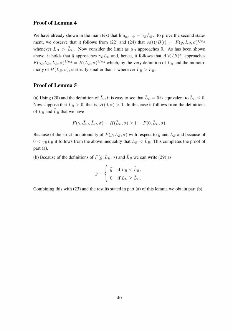
Proof of Lemma 4

We have already shown in the main text that limµB→0 = γBLB. To prove the second state-ment, we observe that it follows from (22) and (24) that A(t)/B(t) = F (g, LB, σ)1/µA

whenever LB > LB. Now consider the limit as µB approaches 0. As has been shownabove, it holds that g approaches γBLB and, hence, it follows that A(t)/B(t) approachesF (γBLB, LB, σ)1/µA = H(LB, σ)1/µA which, by the very definition of LB and the monoto-nicity of H(LB, σ), is strictly smaller than 1 whenever LB > LB.

Proof of Lemma 5

(a) Using (28) and the definition of ¯LB it is easy to see that LB = 0 is equivalent to ¯LB ≤ 0.Now suppose that LB > 0, that is, H(0, σ) > 1. In this case it follows from the definitionsof LB and ¯LB that we have

F (γBLB, LB, σ) = H(LB, σ) ≥ 1 = F (0, ¯LB, σ).

Because of the strict monotonicity of F (g, LB, σ) with respect to g and LB and because of0 < γBLB it follows from the above inequality that LB < ¯LB. This completes the proof ofpart (a).

(b) Because of the definitions of F (g, LB, σ) and ¯LB we can write (29) as

g =

¯g if LB < ¯LB,

0 if LB ≥ ¯LB.

Combining this with (23) and the results stated in part (a) of this lemma we obtain part (b).

40

Working Papers of the Center of Economic Research at ETH Zurich

(PDF-files of the Working Papers can be downloaded at www.cer.ethz.ch/research).

09/118 H. Gersbach, G. Sorger and C. AmonHierarchical Growth: Basic and Applied Research

09/117 C. N. BrunnschweilerFinance for Renewable Energy: An Empirical Analysis of Developing and TransitionEconomies

09/116 S. ValenteOptimal Policy and Non-Scale Growth with R&D Externalities

09/115 T. FahrenbergerShort-term Deviations from Simple Majority Voting

09/114 M. MullerVote-Share Contracts and Learning-by-Doing

09/113 C. Palmer, M. Ohndorf and I. A. MacKenzieLife’s a Breach! Ensuring ’Permanence’ in Forest Carbon Sinks under IncompleteContract Enforcement

09/112 N. Hanley and I. A. MacKenzieThe Effects of Rent Seeking over Tradable Pollution Permits

09/111 I. A. MacKenzieControlling Externalities in the Presence of Rent Seeking

09/110 H. Gersbach and H. HallerClub Theory and Household Formation

09/109 H. Gersbach, V. Hahn and S. ImhofConstitutional Design: Separation of Financing and Project Decision

09/108 C. N. BrunnschweilerOil and Growth in Transition Countries

09/107 H. Gersbach and V. HahnBanking-on-the-Average Rules

09/106 K. Pittel and D.T.G. RubbelkeDecision Processes of a Suicide Bomber – Integrating Economics and Psychology

08/105 A. Ziegler, T. Busch and V.H. HoffmannCorporate Responses to Climate Change and Financial Performance: The Impact ofClimate Policy

09/104 S. ValenteEndogenous Growth, Backstop Technology Adoption and Optimal Jumps

09/103 K. Pittel and D. RubbelkeCharacteristics of Terrorism

09/102 J. DaubanesTaxation of Oil Products and GDP Dynamics of Oil-rich Countries

09/101 S. ValenteAccumulation Regimes in Dynastic Economies with Resource Dependence and HabitFormation

08/100 A. ZieglerDisentangling Specific Subsets of Innovations: A Micro-Econometric Analysis of theirDeterminants

08/99 M. Bambi and A. SaıdiIncreasing Returns to Scale and Welfare: Ranking the Multiple Deterministic Equi-libria

08/98 M. BambiUnifying time-to-build theory

08/97 H. Gersbach and R. WinklerInternational Emission Permit Markets with Refunding

08/96 K. Pittel and L. BretschgerSectoral Heterogeneity, Resource Depletion, and Directed Technical Change: Theoryand Policy

08/95 M. D. Konig, S. Battiston, M. Napoletano and F. SchweitzerThe Efficiency and Evolution of R&D Networks

08/94 H. Gersbach and F. MuheVote-Buying and Growth

08/93 H. GersbachBanking with Contingent Contracts, Macroeconomic Risks, and Banking Crises

08/92 J. DaubanesOptimal taxation of a monopolistic extractor: Are subsidies necessary?

08/91 R. WinklerOptimal control of pollutants with delayed stock accumulation

08/90 S. Rausch and T. F. RutherfordComputation of Equilibria in OLG Models with Many Heterogeneous Households

08/89 E. J. Balistreri, R. H. Hillberry and T. F. RutherfordStructural Estimation and Solution of International TradeModels with Heteroge-neous Firms

08/88 E. Mayer and O. GrimmCountercyclical Taxation and Price Dispersion

08/87 L. BretschgerPopulation growth and natural resource scarcity: long-run development under seem-ingly unfavourable conditions

08/86 M. J. Baker, C. N. Brunnschweiler, and E. H. BulteDid History Breed Inequality? Colonial Factor Endowments and Modern IncomeDistribution

08/85 U. von Arx and A. ZieglerThe Effect of CSR on Stock Performance: New Evidence for the USA and Europe

08/84 H. Gersbach and V. HahnForward Guidance for Monetary Policy: Is It Desirable?

08/83 I. A. MacKenzieOn the Sequential Choice of Tradable Permit Allocations

08/82 I. A. MacKenzie, N. Hanley and T. KornienkoA Permit Allocation Contest for a Tradable Pollution Permit Market

08/81 D. Schiess and R. WehrliThe Calm Before the Storm? - Anticipating the Arrival of General Purpose Tech-nologies

08/80 D. S. Damianov and J. G. BeckerAuctions with Variable Supply: Uniform Price versus Discriminatory

08/79 H. Gersbach, M. T. Schneider and O. SchnellerOn the Design of Basic-Research Policy

08/78 C. N. Brunnschweiler and E. H. BulteNatural Resources and Violent Conflict: Resource Abundance, Dependence and theOnset of Civil Wars

07/77 A. Schafer, S. ValenteHabit Formation, Dynastic Altruism, and Population Dynamics

07/76 R. WinklerWhy do ICDPs fail? The relationship between subsistence farming, poaching andecotourism in wildlife and habitat conservation

07/75 S. ValenteInternational Status Seeking, Trade, and Growth Leadership

07/74 J. Durieu, H. Haller, N. Querou and P. SolalOrdinal Games

07/73 V. HahnInformation Acquisition by Price-Setters and Monetary Policy

07/72 H. Gersbach and H. HallerHierarchical Trade and Endogenous Price Distortions