Ceres SolverConvenient Fast Non-linear Optimzation

Mikael Persson

Department of Electrical EngineeringComputer Vision Laboratory

Linkoping University

May 18, 2015

Ceres Solver

Introduction

Non-linear optimization library

• Convenient - good api, automatic symbolic differentiation

• Fast, in particular if used with Suitesparse and the correct blas

• Powerful/semi generic

• Well documented and straightforward installation in Linux.

2

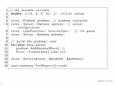
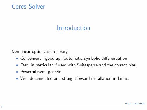
1 // the mutable v a r i a b l e2 double∗ x={1, 2 , 3 , 4} ; // , i n i t i a l v a l u e s34 c e r e s : : Problem problem ; // problem c o n t a i n e r5 c e r e s : : S o l v e r : : Opt ions o p t i o n s ; // s o l v e r

c o n f i g u r a t i o n6 c e r e s : : Lo s sFunc t i on ∗ l o s s=n u l l p t r ; // i i d gauss7 c e r e s : : S o l v e r : : Summary summary ;89 // b u i l d the problem/ co s t

10 f o r ( auto data : da ta s )11 problem . AddRes idua lB lock ( \\12 E r r o r : : C rea te ( data ) , Loss , x ) ) ;1314 c e r e s : : So l v e ( op t i on s , &problem , &summary ) ;1516 cout<<summary . Fu l l R e po r t ( )<<end l ;

3

Ceres Solver

Lossfunctions

Several types of loss functions are available.

• What noise is assumed

• Consider the usecases

• Influence on convergence?

Most twice derivable functions with a continuous derivative areeasy to implement.

4

Ceres Solver

Solver Options

The most useful options are:

• Solver type

• convergence/exit criteria

Parameter Block Order:

• Sparsity and elimination order information

• Guessed if not specified

• Significant performance gains possible

5

cvl & mlib

CVL has a linear algebra lib

• Developed by Hedborg

• Similar to eigen

• Vector2,3,4

• Matrix3x3 to Matrix 4x4

• Common operations available

mlib extras

• quaternions

• poses(rigid transforms)

• dynamic states(cv,ca,cea, osv)

• uniformly sampled random rotations

6

cvl & mlib

CVL has a linear algebra lib

Why?

• Simpler to modify cvl than eigen

• operator ∗ (X < double >,Y < ceres :: jet >)

• ceres::jet is the ceres differentiation wrapper

7

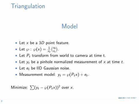
Triangulation

Model

• Let x be a 3D point feature.

• Let ℘ : ℘(x) = 1x2

(x0x1

).

• Let Pt transform from world to camera at time t.

• Let yt be a pinhole normalized measurement of x at time t.

• Let et be IID Gaussian noise.

• Measurement model: yt = ℘(Ptx) + et .

Minimize:∑

(yt − ℘(Ptx))2 over x .

8

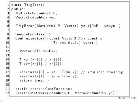
1 c l a s s Tr i gE r r o r {2 pub l i c :3 Matr ix4x4<double> P ;4 Vector2<double> yn ;56 T r i gE r r o r ( Matr i x4x4 P , Vector2 yn ) {P=P ; yn=yn ;}78 template<c l a s s T>9 bool operator ( ) ( const Vector3<T>∗ const x ,

10 T∗ r e s i d u a l s ) const {1112 Vector3<T> x r=P∗x ;1314 T xp=(x r [ 0 ] / x r [ 2 ] ) ;15 T yp=(x r [ 1 ] / x r [ 2 ] ) ;1617 r e s i d u a l s [ 0 ] = xp − T( yn . x ) ; // i m p l i c i t s q u a r i n g18 r e s i d u a l s [ 1 ] = yp − T( yn . y ) ;19 re tu rn t rue ; }2021 s t a t i c c e r e s : : Cos tFunc t i on ∗22 Crea te ( Matr ix4x4<double> P, Vector2<double> yn ) ; } ;

9

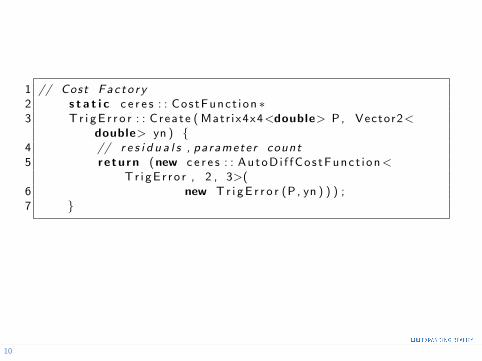
1 // Cost Fac to r y2 s t a t i c c e r e s : : Cos tFunc t i on ∗3 T r i gE r r o r : : C rea te ( Matr ix4x4<double> P, Vector2<

double> yn ) {4 // r e s i d u a l s , pa ramete r count5 re tu rn (new c e r e s : : AutoD i f fCos tFunc t i on<

Tr i gE r r o r , 2 , 3>(6 new Tr i gE r r o r (P , yn ) ) ) ;7 }

10

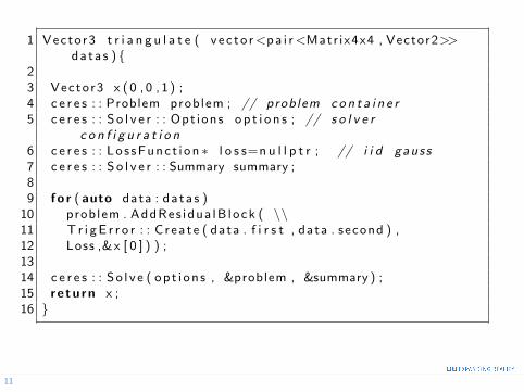
1 Vector3 t r i a n g u l a t e ( vec to r<pa i r<Matr ix4x4 , Vector2>>da ta s ) {

23 Vector3 x (0 , 0 , 1 ) ;4 c e r e s : : Problem problem ; // problem c o n t a i n e r5 c e r e s : : S o l v e r : : Opt ions o p t i o n s ; // s o l v e r

c o n f i g u r a t i o n6 c e r e s : : Lo s sFunc t i on ∗ l o s s=n u l l p t r ; // i i d gauss7 c e r e s : : S o l v e r : : Summary summary ;89 f o r ( auto data : da ta s )

10 problem . AddRes idua lB lock ( \\11 T r i gE r r o r : : C rea te ( data . f i r s t , data . second ) ,12 Loss ,&x [ 0 ] ) ) ;1314 c e r e s : : So l v e ( op t i on s , &problem , &summary ) ;15 re tu rn x ;16 }

11

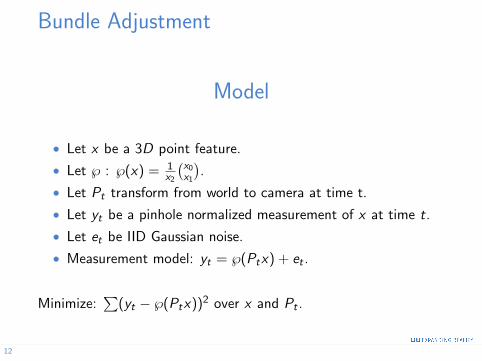
Bundle Adjustment

Model

• Let x be a 3D point feature.

• Let ℘ : ℘(x) = 1x2

(x0x1

).

• Let Pt transform from world to camera at time t.

• Let yt be a pinhole normalized measurement of x at time t.

• Let et be IID Gaussian noise.

• Measurement model: yt = ℘(Ptx) + et .

Minimize:∑

(yt − ℘(Ptx))2 over x and Pt .

12

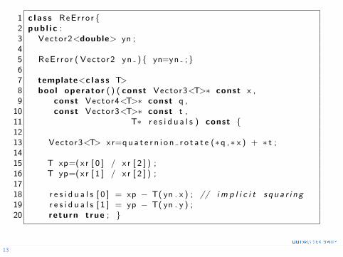
1 c l a s s ReEr ro r {2 pub l i c :3 Vector2<double> yn ;45 ReEr ro r ( Vector2 yn ) { yn=yn ;}67 template<c l a s s T>8 bool operator ( ) ( const Vector3<T>∗ const x ,9 const Vector4<T>∗ const q ,

10 const Vector3<T>∗ const t ,11 T∗ r e s i d u a l s ) const {1213 Vector3<T> x r=q u a t e r n i o n r o t a t e (∗q ,∗ x ) + ∗ t ;1415 T xp=(x r [ 0 ] / x r [ 2 ] ) ;16 T yp=(x r [ 1 ] / x r [ 2 ] ) ;1718 r e s i d u a l s [ 0 ] = xp − T( yn . x ) ; // i m p l i c i t s q u a r i n g19 r e s i d u a l s [ 1 ] = yp − T( yn . y ) ;20 re tu rn t rue ; }

13

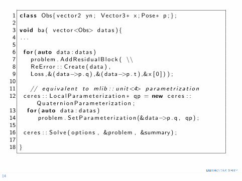
1 c l a s s Obs{ v e c t o r 2 yn ; Vector3 ∗ x ; Pose∗ p ; } ;23 vo id ba ( vec to r<Obs> da ta s ) {4 . . .56 f o r ( auto data : da ta s )7 problem . AddRes idua lB lock ( \\8 ReEr ro r : : C rea te ( data ) ,9 Loss ,&( data−>p . q ) ,&( data−>p . t ) ,&x [ 0 ] ) ) ;

1011 // e q u i v a l e n t to ml ib : : un i t<4> p a r ame t r i z a t i o n12 c e r e s : : L o c a lP a r ame t e r i z a t i o n ∗ qp = new c e r e s : :

Qua t e r n i o nPa r ame t e r i z a t i o n ;13 f o r ( auto data : da ta s )14 problem . S e tPa r ame t e r i z a t i o n (&data−>p . q , qp ) ;1516 c e r e s : : So l v e ( op t i on s , &problem , &summary ) ;1718 }

14

• This is how to get you started.

• There are excellent guides available online

• Great performance gains by manual specification of sparsityand elimination order. Dont try that first though!

• Questions?

15