CFAR PROCESSING WITH MULTIPLE EXPONENTIAL SMOOTHERS FORNONHOMOGENEOUS ENVIRONMENTS

A THESIS SUBMITTED TOTHE GRADUATE SCHOOL OF NATURAL AND APPLIED SCIENCES

OFMIDDLE EAST TECHNICAL UNIVERSITY

BY

BERK GURAKAN

IN PARTIAL FULFILLMENT OF THE REQUIREMENTSFOR

THE DEGREE OF MASTER OF SCIENCEIN

ELECTRICAL AND ELECTRONICS ENGINEERING

DECEMBER 2010

Approval of the thesis:

CFAR PROCESSING WITH MULTIPLE EXPONENTIAL SMOOTHERS FOR

NONHOMOGENEOUS ENVIRONMENTS

submitted byBERK GURAKAN in partial fulfillment of the requirements for the degree ofMaster of Science in Electrical and Electronics Engineering Department, Middle EastTechnical University by,

Prof. Dr. CananOzgenDean, Graduate School ofNatural and Applied Sciences

Prof. Dr. Ismet ErkmenHead of Department,Electrical and Electronics Engineering

Assoc. Prof. Dr. Tolga CilogluSupervisor,Electrical and Electronics Engineering Dept., METU

Assoc. Prof. Dr. Cagatay CandanCo-supervisor,Electrical and Electronics Engineering Dept., METU

Examining Committee Members:

Prof. Dr. Mubeccel DemireklerElectrical and Electronics Engineering Dept., METU

Assoc. Prof. Dr. Tolga CilogluElectrical and Electronics Engineering Dept., METU

Prof. Dr. Mustafa KuzuogluElectrical and Electronics Engineering Dept., METU

Prof. Dr. Aydın AlatanElectrical and Electronics Engineering Dept., METU

Serkan Ceylan (M.Sc.)ASELSAN

Date:

I hereby declare that all information in this document has been obtained and presentedin accordance with academic rules and ethical conduct. I also declare that, as requiredby these rules and conduct, I have fully cited and referenced all material and results thatare not original to this work.

Name, Last Name: BERK GURAKAN

Signature :

iii

ABSTRACT

CFAR PROCESSING WITH MULTIPLE EXPONENTIAL SMOOTHERS FORNONHOMOGENEOUS ENVIRONMENTS

Gurakan, Berk

M.Sc., Department of Electrical and Electronics Engineering

Supervisor : Assoc. Prof. Dr. Tolga Ciloglu

Co-Supervisor : Assoc. Prof. Dr. Cagatay Candan

December 2010, 84 pages

Conventional methods of CFAR detection always use windowing, in the sensethat some

number of cells are investigated and the target present/absent decision is made according to

the composition of the cells in that window. The most commonly used versions of CFAR

detection algorithms are cell averaging CFAR, smallest of cell averaging CFAR, greatest of

cell averaging CFAR and order-statistics CFAR. These methods all use windowing to set

the decision threshold. In this thesis, rather than using windowed CFAR algorithms, a new

method of estimating the background threshold is presented, analyzed and simulated. This

new method is called the Switching IIR CFAR algorithm and uses two IIR filters to accurately

estimate the background threshold. Then, using a comparison procedure, one of the filters is

selected as the current threshold estimate and used. The results are seento be satisfactory and

comparable to conventional CFAR methods. The basic advantages of usingthe SIIR CFAR

method are computational simplicity, small memory requirement and acceptable performance

under clutter edges and multiple targets.

Keywords: CFAR, IIR Filter, Radar, Detection, Switching

iv

OZ

RADAR HEDEF TESPITINDE FILTRELEME YONTEMLERININ KULLANIMI

Gurakan, Berk

Yuksek Lisans, Elektrik ve Elektronik Muhendisligi Bolumu

Tez Yoneticisi : Doc. Dr. Tolga Ciloglu

Ortak Tez Yoneticisi : Doc. Dr. Cagatay Candan

Aralık 2010, 84 sayfa

Sabit yanlıs alarm olasılıgı (SYAO) yontemleri genelde birden cok hucreye bakıp, bu hucrelerin

belirli istatistikselozelliklerine gore (ortalama, minimum, maksimum vs) tespit esigini be-

lirlemektedirler. Bu da, hem hafıza gereksinimi acısından hem de islem yuku acısından

belirli problemleri beraberinde getirmektedir. Bu calısmada, iki tane sonsuz durtu cevaplı

filtre kullanılarak tespit esigi kestirilmistir. Belirli bir karsılastırma isleminden sonra hangi

filtrenin secilecegine karar veren bir algoritma gelistirilmistir. Bu filtreler yalnızca tek bir

hucreye bakarak calıstıkları icin islem yuku ve hafıza gereksinimi acısından bilinen SYAO

yontemlerinden daha iyilerdir. Bu algoritmanın simulasyon sonuclarının bilinen SYAO

yontemlerine yakın oldugu gorulmustur.

Anahtar Kelimeler: Radar, Filtre, Sonsuz Durtu Cevabı

v

To My Family

vi

ACKNOWLEDGMENTS

I would like to express my deepest gratitude to my supervisor Assoc. Prof.Dr. Tolga Ciloglu

for his guidance, advice, criticism, encouragements and insight throughout the research.

I would also like to thank my co advisor Assoc. Prof. Dr. Cagatay Candan for his valuable

remarks and thoughtful comments. He has made his support available in a number of ways.

Thanks to the examining committee members Prof. Dr. Mubeccel Demirekler, Prof. Dr.

Mustafa Kuzuoglu, Prof. Dr. Aydın Alatan and Serkan Ceylan for evaluating my work and

for their valuable comments.

I would like to express my gratitude to Oktay Sipahigil for his excellent suggestions and sup-

port.

Deepest thanks to my family for their love, trust and understanding.

vii

TABLE OF CONTENTS

ABSTRACT . . . . . . . . . . . . . . . . . . . . . . . . . . . . . . . . . . . . . . . . iv

OZ . . . . . . . . . . . . . . . . . . . . . . . . . . . . . . . . . . . . . . . . . . . . . v

ACKNOWLEDGMENTS . . . . . . . . . . . . . . . . . . . . . . . . . . . . . . . . . vii

TABLE OF CONTENTS . . . . . . . . . . . . . . . . . . . . . . . . . . . . . . . . . viii

LIST OF TABLES . . . . . . . . . . . . . . . . . . . . . . . . . . . . . . . . . . . . xi

LIST OF FIGURES . . . . . . . . . . . . . . . . . . . . . . . . . . . . . . . . . . . . xii

CHAPTERS

1 INTRODUCTION . . . . . . . . . . . . . . . . . . . . . . . . . . . . . . . 1

1.1 Scope . . . . . . . . . . . . . . . . . . . . . . . . . . . . . . . . . . 1

1.2 Outline . . . . . . . . . . . . . . . . . . . . . . . . . . . . . . . . . 2

1.3 Detection Fundamentals . . . . . . . . . . . . . . . . . . . . . . . . 2

1.3.1 The Neyman-Pearson Criterion . . . . . . . . . . . . . . . 3

1.3.2 The Likelihood Ratio Test . . . . . . . . . . . . . . . . . 4

1.3.3 Coherent Detection . . . . . . . . . . . . . . . . . . . . . 10

1.3.4 Unknown parameters . . . . . . . . . . . . . . . . . . . . 13

1.3.5 Radar Signal Detection . . . . . . . . . . . . . . . . . . . 17

2 CONSTANT FALSE ALARM RATE DETECTION . . . . . . . . . . . . . . 21

2.1 Case of Unknown Interference Power . . . . . . . . . . . . . . . . . 21

viii

2.2 Types of CFAR Processors . . . . . . . . . . . . . . . . . . . . . . 22

2.2.1 Cell Averaging CFAR . . . . . . . . . . . . . . . . . . . . 22

2.2.2 Smallest-of-Cell-Averaging CFAR . . . . . . . . . . . . . 27

2.2.3 Greater-of-cell-averaging CFAR . . . . . . . . . . . . . . 29

2.2.4 Censored or Trimmed mean CFAR . . . . . . . . . . . . . 30

2.2.5 Order Statistic CFAR . . . . . . . . . . . . . . . . . . . . 31

2.2.6 Variability Index CFAR . . . . . . . . . . . . . . . . . . . 34

2.2.7 Switching CFAR . . . . . . . . . . . . . . . . . . . . . . 36

2.2.8 Log CFAR . . . . . . . . . . . . . . . . . . . . . . . . . 36

2.2.9 Adaptive CFAR . . . . . . . . . . . . . . . . . . . . . . . 38

2.2.10 Clutter Map CFAR . . . . . . . . . . . . . . . . . . . . . 39

2.2.11 Other CFAR types . . . . . . . . . . . . . . . . . . . . . 40

3 CFAR DETECTION USING IIR FILTERS . . . . . . . . . . . . . . . . . . 41

3.1 Proposed Algorithm . . . . . . . . . . . . . . . . . . . . . . . . . . 48

3.2 Calculation ofTS . . . . . . . . . . . . . . . . . . . . . . . . . . . 50

4 SIMULATION RESULTS . . . . . . . . . . . . . . . . . . . . . . . . . . . 60

4.1 False alarm probability under homogeneous conditions . . . . . . . 60

4.2 False alarm probability under clutter edge . . . . . . . . . . . . . . 61

4.2.1 Simulation Setup . . . . . . . . . . . . . . . . . . . . . . 61

4.2.2 Simulation Results . . . . . . . . . . . . . . . . . . . . . 63

4.2.2.1 Effect of varyingPFA . . . . . . . . . . . . . 64

4.2.2.2 Effect of varyingPFS . . . . . . . . . . . . . 67

4.2.2.3 Effect of varyingN1 . . . . . . . . . . . . . . 68

ix

4.2.2.4 Effect of varying CNR . . . . . . . . . . . . . 70

4.3 Probability of detection under homogeneous conditions . . . . . . . 71

4.3.1 Simulation Setup . . . . . . . . . . . . . . . . . . . . . . 71

4.3.2 Simulation Results . . . . . . . . . . . . . . . . . . . . . 72

4.3.2.1 Effect of varyingPFA . . . . . . . . . . . . . 72

4.3.2.2 Effect of varyingN1 . . . . . . . . . . . . . . 73

4.3.2.3 Effect of varyingPFS . . . . . . . . . . . . . 74

4.4 Probability of detection under interfering targets . . . . . . . . . . . 76

4.5 Comparison to other CFAR Algorithms . . . . . . . . . . . . . . . . 77

5 CONCLUSION . . . . . . . . . . . . . . . . . . . . . . . . . . . . . . . . . 79

REFERENCES . . . . . . . . . . . . . . . . . . . . . . . . . . . . . . . . . . . . . . 82

x

LIST OF TABLES

TABLES

Table 2.1 VI CFAR adaptive threshold selection . . . . . . . . . . . . . . . . . . .. 36

Table 3.1 The linear multiplier forN2 = 256 andN1 for {16,32,64,128} to achieve a

desiredPFS . . . . . . . . . . . . . . . . . . . . . . . . . . . . . . . . . . . . . 58

xi

LIST OF FIGURES

FIGURES

Figure 1.1 Detector setup for a known constant in Gaussian noise . . . . . .. . . . . 10

Figure 1.2 Detector setup for a known constant with unknown phase in Gaussian noise 17

Figure 1.3 Detector setup for nonfluctuating targets and corresponding pdfs underH0 19

Figure 2.1 General CFAR Detector scheme . . . . . . . . . . . . . . . . . . . . . .. 22

Figure 2.2 CFAR reference window.xi is the cell under test (CUT) . . . . . . . . . . 24

Figure 2.3 CA CFAR threshold behavior and clutter edge performance . . .. . . . . 27

Figure 2.4 SOCA CFAR threshold behavior and clutter edge performance . .. . . . . 28

Figure 2.5 GOCA CFAR threshold behavior and clutter edge performance . .. . . . 30

Figure 2.6 CMLD threshold behavior and clutter edge performance . . . . .. . . . . 32

Figure 2.7 OS CFAR threshold behavior and clutter edge performance, k=10th statis-

tic is used . . . . . . . . . . . . . . . . . . . . . . . . . . . . . . . . . . . . . . 33

Figure 2.8 VI CFAR Block Diagram . . . . . . . . . . . . . . . . . . . . . . . . . . 35

Figure 2.9 log CFAR threshold behavior and clutter edge performance . . .. . . . . 37

Figure 2.10 Adaptive CFAR threshold behaviour and clutter edge performance . . . . . 39

Figure 3.1 The IIR Filter Detector . . . . . . . . . . . . . . . . . . . . . . . . . . . . 41

Figure 3.2 Detection using an IIR Filter . . . . . . . . . . . . . . . . . . . . . . . . . 42

xii

Figure 3.3 PD vs SNR curves for CA CFAR and IIR CFAR for differentN values and

equivalentγ parameters . . . . . . . . . . . . . . . . . . . . . . . . . . . . . . . 45

Figure 3.4 Threshold behaviour of IIR CFAR . . . . . . . . . . . . . . . . . . .. . . 46

Figure 3.5 Threshold behavior of IIR CFAR under a clutter edge . . . . . .. . . . . 47

Figure 3.6 Different behaviors of two filters under a clutter edge . . . . . . . . . . . . 48

Figure 3.7 PFS simulations forN1 = 16 andN2 = 256 . . . . . . . . . . . . . . . . . 55

Figure 3.8 PFS simulations forN1 = 32 andN2 = 256 . . . . . . . . . . . . . . . . . 56

Figure 3.9 PFS simulations forN1 = 64 andN2 = 256 . . . . . . . . . . . . . . . . . 56

Figure 3.10PFS simulations forN1 = 128 andN2 = 256 . . . . . . . . . . . . . . . . 57

Figure 3.11 The SIIR CFAR algorithm explained . . . . . . . . . . . . . . . . . . .. 58

Figure 3.12 Block diagram implementation of the switching algorithm . . . . . . . . . 59

Figure 3.13 SIIR CFAR at work . . . . . . . . . . . . . . . . . . . . . . . . . . . . .59

Figure 4.1 Pfa for SIIR CFAR under homogeneous environment . . . . . .. . . . . . 61

Figure 4.2 Pfa under clutter edge simulation setup . . . . . . . . . . . . . . . . . . .62

Figure 4.3 PFA simulations under clutter edge forN1 = 32, N2 = 256, PFA =

10−2,CNR= 10dB,PFS = 10−4 . . . . . . . . . . . . . . . . . . . . . . . . . . . 64

Figure 4.4 PFA simulations under clutter edge forN1 = 32, N2 = 256, PFA =

10−3,CNR= 10dB,PFS = 10−4 . . . . . . . . . . . . . . . . . . . . . . . . . . . 64

Figure 4.5 PFA simulations under clutter edge forN1 = 32, N2 = 256, PFA =

10−4,CNR= 10dB,PFS = 10−4 . . . . . . . . . . . . . . . . . . . . . . . . . . . 65

Figure 4.6 PFA simulations under clutter edge forN1 = 32, N2 = 256, PFA =

10−5,CNR= 10dB,PFS = 10−4 . . . . . . . . . . . . . . . . . . . . . . . . . . . 65

Figure 4.7 PFA simulations under clutter edge forN1 = 32, N2 = 256, PFA =

10−6,CNR= 10dB,PFS = 10−4 . . . . . . . . . . . . . . . . . . . . . . . . . . . 66

xiii

Figure 4.8 PFA simulations under clutter edge forN1 = 32, N2 = 256, PFA =

10−4,CNR= 10dB,PFS = 10−3 . . . . . . . . . . . . . . . . . . . . . . . . . . . 67

Figure 4.9 PFA simulations under clutter edge forN1 = 32, N2 = 256, PFA =

10−4,CNR= 10dB,PFS = 10−5 . . . . . . . . . . . . . . . . . . . . . . . . . . . 67

Figure 4.10PFA simulations under clutter edge forN1 = 64, N2 = 256, PFA =

10−4,CNR= 10dB,PFS = 10−4 . . . . . . . . . . . . . . . . . . . . . . . . . . . 68

Figure 4.11PFA simulations under clutter edge forN1 = 128, N2 = 256, PFA =

10−4,CNR= 10dB,PFS = 10−4 . . . . . . . . . . . . . . . . . . . . . . . . . . . 69

Figure 4.12PFA simulations under clutter edge forN1 = 32, N2 = 256, PFA =

10−4,CNR= 5dB, PFS = 10−4 . . . . . . . . . . . . . . . . . . . . . . . . . . . . 70

Figure 4.13PFA simulations under clutter edge forN1 = 32, N2 = 256, PFA =

10−4,CNR= 7dB, PFS = 10−4 . . . . . . . . . . . . . . . . . . . . . . . . . . . . 70

Figure 4.14PD simulations forN1 = 32, N2 = 256, PFA = 10−4, PFS = 10−4 under

homogeneous conditions . . . . . . . . . . . . . . . . . . . . . . . . . . . . . . . 72

Figure 4.15PD simulations forN1 = 32, N2 = 256, PFA = 10−5, PFS = 10−4 under

homogeneous conditions . . . . . . . . . . . . . . . . . . . . . . . . . . . . . . . 72

Figure 4.16PD simulations forN1 = 32, N2 = 256, PFA = 10−6, PFS = 10−4 under

homogeneous conditions . . . . . . . . . . . . . . . . . . . . . . . . . . . . . . . 73

Figure 4.17PD simulations forN1 = 64, N2 = 256, PFA = 10−4, PFS = 10−4 under

homogeneous conditions . . . . . . . . . . . . . . . . . . . . . . . . . . . . . . . 73

Figure 4.18PD simulations forN1 = 128,N2 = 256,PFA = 10−4, PFS = 10−4 under

homogeneous conditions . . . . . . . . . . . . . . . . . . . . . . . . . . . . . . . 74

Figure 4.19PD simulations forN1 = 32, N2 = 256, PFA = 10−4, PFS = 10−1 under

homogeneous conditions . . . . . . . . . . . . . . . . . . . . . . . . . . . . . . . 74

Figure 4.20PD simulations forN1 = 32, N2 = 256, PFA = 10−4, PFS = 10−2 under

homogeneous conditions . . . . . . . . . . . . . . . . . . . . . . . . . . . . . . . 75

xiv

Figure 4.21 Simulation setup for multiple targets . . . . . . . . . . . . . . . . . . . . 76

Figure 4.22PD simulations forN1 = 32, N2 = 256, PFA = 10−4, PFS = 10−4 under

one interfering target 0.5 second away . . . . . . . . . . . . . . . . . . . . . . . 77

Figure 4.23PFA simulations under clutter edge for SIIR CFAR vs. other known CFAR

algorithms . . . . . . . . . . . . . . . . . . . . . . . . . . . . . . . . . . . . . . 78

xv

CHAPTER 1

INTRODUCTION

Classical hypothesis testing aims to decide between the null hypothesis and thealternative

hypothesis. These hypotheses can be a statistical induction statement (such as ”all cars are

red”) or in the context of a radar, a target present or absent decision. There are many different

ways to develop statistical tests to decide which one of these hypotheses arecorrect. One of

the first developments in hypothesis testing was initiated by Bayes [1] and Neyman-Pearson

[2] have contributed significantly to the field later on.

If the hypotheses are regarded in terms of signal present or absent decision, the problem can

be called binary signal detection. It is called binary in the sense that there are two possible

hypotheses, either a 1 or a 0. In this thesis, only binary signal detection willbe considered

even though M-ary signal detection (more than two hypotheses) is also citedfrequently in

literature.

1.1 Scope

The aim of this work is to present a new algorithm for constant false alarm rate (CFAR) detec-

tion of radar targets under Gaussian noise, based on an IIR filtering andswitching approach.

The performance of this detector will be analyzed by simulations and theoretical calculations.

Signals are modeled as exponential random variables (the Swerling model) and the noise is

modeled as a white Gaussian process.

1

1.2 Outline

In 1.3, a review of detection theory is made which will be used in later parts of the thesis. In

Chapter 2, a literature review on constant false alarm rate (CFAR) processing is made. Com-

monly used CFAR methods are explained with examples, equations and figures.In Chapter

3, CFAR detection using IIR filters is explained and the proposed algorithm together with

the modifications and reasoning is presented. In Chapter 4, the simulation results and com-

ments about the results are given. In Chapter 5, the thesis is concluded withfinishing remarks,

summary and an outline of future work.

1.3 Detection Fundamentals

The primary functions of any surveillance system (radar, sonar etc) are detection, tracking

and imaging. The main concern here is to decide whether any measurement falls into one of

the two categories:

1. The measurement is the result of interference (noise) only.

2. The measurement is the combined result of interference and echoes from a target.

The first hypothesis is denoted as thenull hypothesis, H0 and the second asalternative hypoth-

esis H1. The detector must use some kind of logic that determines whether a measurement

falls underH0 or H1. If H0 best accounts for the data, the system declares that no target was

present for that measurement. IfH1 best accounts for the data, the system declares that a target

was present for that certain measurement. Since the signals can only be described statistically,

the decision between the two hypotheses is a matter of statistical decision theory. One should

start the analysis using a probability density function (pdf) describing the measurement to be

tested under each of the two hypotheses. Let the sample to be denoted asy, then the following

definitions are valid:

2

py(y|H0) = the pdf of y given that a target was not present (H0 is true)

py(y|H1) = the pdf of y given that a target was present (H1 is true)

More generally, the detection will be based on not a single sample butN number of samples

of datayn forming a vectory

y ≡ [y0 . . . yN−1]

TheN dimensional joint pdfspy(y|H0) andpy(y|H1) are then used. The following probabilities

are important and must be defined here:

Probability of Detection (PD): The probability that a targetis declared(H1 is chosen) when a

targetis in fact present.

Probability of False Alarm (PFA): The probability that a targetis declared (H1 is chosen)

when a target is in factnot present.

Probability of Miss (PM): The probability that a target isnot declared (H0 is chosen) when a

targetis in fact present.

SincePM = 1− PD, PFA andPD are sufficient to specify all of the probabilities of interest.

1.3.1 The Neyman-Pearson Criterion

The next step in decision making is to find a rule for deciding what makes an optimal choice

between the two hypotheses. The approaches follow directly from the theory of simple hy-

pothesis testing problem. There are two main methods for dealing with this problem,the

Neyman-Pearson criterion and the Bayesian risk approach. Sonar andradar systems typically

use the Neyman-Pearson criterion [3]. The Neyman-Pearson criterion aims to find a decision

process to maximize the probability of detectionPD under the constraint that the false alarm

probabilityPFA does not exceed a certain number. This criterion is motivated by the fact that

for a fixed system design, increasingPD implies increasingPFA as well [4].

3

Each vector of measured data valuesy is a point inN dimensional space. To have a complete

decision rule, every possible point in that space must be assigned to one of the hypotheses,

H0 (”target absent”) orH1 (”target present”). LetR1 denote the region for which ify ∈ R1

we denote target present (i.e,H1). This means that the regionR1 is mapped toH1. Then, the

following definitions are valid:

PD =

∫

R1

py(y|H1) dy

PFA =

∫

R1

py(y|H0) dy (1.1)

Since probability density functions are nonnegative, it is seen from (1.1)that PD and PFA

must rise or fall together whenR1 changes. Obviously whenR1 grows to include more of the

possible observationsy, both of the integrals will be larger because of the nonnegative pdf.

This leads to a very important result, in order to increase the detection probability, the false

alarm probability must be allowed to increase as well.

1.3.2 The Likelihood Ratio Test

The Neyman-Pearson criterion aims to obtain the best possible detection performance while

keeping a tolerable false alarm probability. This can be mathematically formulatedas follows:

chooseR1 such thatPD is maximized, subject toPFA ≤ α

whereα is the maximum tolerable false alarm probability. One can use the method of La-

grange multipliers to solve this optimization problem. LetF be defined as

F = PD + λ(PFA − α)

Now the problem is maximizingF and then choosingλ to satisfyPFA = α. Substituting from

(1.1) we get:

4

maxF = max{∫

R1

py(y|H1) dy + λ(∫

R1

py(y|H0) dy − α)}

= max{−λα +∫

R1

py(y|H1) + λpy(y|H0) dy} (1.2)

The first term of (1.2) does not depend on the choice ofR1 therefore it can be omitted in the

maximization process. To maximizeF, one needs to maximize the value of the integral over

R1. So we should includey in R1 if the integrand is positive for that value ofy. This means

R1 must be made of pointsy for which

py(y|H1) + λpy(y|H0) > 0

This directly leads to the decision rule

py(y|H1)

py(y|H0)

H1

≷H0

−λ (1.3)

(1.3) is known as thelikelihood ratio test (LRT). This test is very useful in the sense that

it gives an optimal rule for guessing, under the Neyman-Pearson criterion, whether a target

is present or not based directly on the observed datay and the threshold−λ. Note that this

threshold still needs to be computed. This threshold should be computed usingthePFA con-

straint. (1.3) tells us that the ratio of two pdfs, evaluated for the particular observationy, must

be computed and if that ”likelihood ratio” exceeds some threshold, a target present decision

must be made (chooseH1). If it does not exceed the threshold, declare no target is present

(chooseH0). To carry out the LRT, it is obvious that the models ofpy(y|H1) andpy(y|H0) are

needed. As a convenient way, the LRT can be expressed in the followingnotation:

Λ(y)H1

≷H0

η (1.4)

From (1.3),Λ(y) =py(y|H1)py(y|H0) andη = −λ. One can apply a monotone increasing operator to

both sides of (1.4) and this will not change the performance. Most common way is to take

natural logarithm to obtain thelog likelihood ratio test.

5

lnΛ(y)H1

≷H0

ln η (1.5)

To illustrate these cases better, consider a simple case where the presenceor absence of a con-

stant, in zero-mean Gaussian noise of varianceβ2 is to be decided. This means distinguishing

between two hypotheses:

H0 : y = w

H1 : y = m + w

wherew is a vector of independent identically distributed (i.i.d) zero mean Gaussian random

variables andm is a vector of constants. When there is no signal (hypothesisH0) the data

vector y has anN-dimensional normal distribution with covariance matrixβ2I N where I N

is the identity matrix of dimensionsN × N. When there is a signal (hypothesisH1), the

distribution is simply shifted to a nonzero mean.

H0 : y ∼ N(0N , β2I N)

H1 : y ∼ N(mN , β2I N) (1.6)

The joint pdf ofy under both hypothesis is therefore

py(y|H0) =N−1∏

n=0

1√2πβ2

exp{−12

(yn

β)2}

py(y|H1) =N−1∏

n=0

1√2πβ2

exp{−12

(yn − mβ

)2} (1.7)

The likelihood ratioΛ(y) and the log likelihood ratio can be directly calculated.

6

Λ(y) =py(y|H1)

py(y|H0)=

∏N−1n=0

1√2πβ2

exp{−12( ynβ

)2}∏N−1

n=01√2πβ2

exp{−12( yn−m

β)2}

(1.8)

lnΛ(y) =N−1∑

n=0

{−12

(yn − mβ

)2 +12

(yn

β)2}

=1β2

N−1∑

n=0

myn −1

2β2

N−1∑

n=0

m2 (1.9)

Using the log likelihood ratio and (1.5) we arrive at the following result.

N−1∑

n=0

yn

H1

≷H0

β2

mln (−λ) + Nm

2(1.10)

It is worth noting that right hand side of (1.10) does not depend onyn and can therefore be

considered as a constant. It is specified from this equation that the available data samples,

yn, must be summed and then compared to a detection threshold, which still needs tobe

computed. This is an example of how LRT specifies the signal processing required on the

data, to achieve optimal detection performance. In most cases, the LRT canbe rearranged to

isolate on one hand, only these terms including the data samples, moving all otherconstants

to the other hand side. The term∑

yn is called thesufficient statistic for this example and

denoted byΥ(y). The sufficient statistic is a function of the datay and has the property that

the likelihood ratio can be written as a function ofΥ(y). This means that no other statistic

which can be calculated from the same sample, provides any additional information. This also

means that knowing the sufficient statistic is as good as knowing the data itself [5]. Therefore,

the LRT can now be changed to:

Υ(y)H1

≷H0

T (1.11)

Note that (1.11) is in the form of (1.10) withΥ(y) =∑

yn andT = β2

m ln(−λ) + Nm2 .

SinceΛ andΥ are functions of the data vectory, they have their own pdfs. This means we

can compute the LRT threshold in terms ofΛ andΥ to compute the detection threshold. One

can use the following expressions:

7

PFA =

∫ ∞

η=−λpΛ(Λ|H0) dΛ = α

PFA =

∫ ∞

TpΥ(Υ|H0) dΥ = α (1.12)

Continuing from the same example, we saw that the sufficient statisticΥ(y) is just the sum of

the data samplesyn, Υ =∑N−1

i=0 yn. UnderH0, yn ∼ N(0, β2) and thereforeΥ ∼ N(0,Nβ2).

Using the definitions in (1.12) we arrive at the following results.

PFA =

∫ ∞

TpΥ(Υ|H0) dΥ = α

=

∫ ∞

T

1√2πNβ2

e− Υ2

2Nβ2 dΥ (1.13)

Define theerror function, erf(x) andcomplementary error function, erfc(x) as:

erf(x) =2√π

∫ x

0e−t2 dt (1.14)

erfc(x) =2√π

∫ ∞

xe−t2 dt (1.15)

It can be seen that erfc(x) = 1− erf(x). One also needs to define the inverse error and inverse

complementary error functions, and these are defined as erf-1(x) and erfc-1(x). It can be shown

that erfc-1(x) = erf-1(1− x).

To evaluate the integral in (1.13), make the change of variablest =Υ√

2Nβ2, then

dt =dΥ√2Nβ2

PFA =1√π

∫ ∞

T/√

2Nβ2e−t2 dt = α

=12

1− erf

T√

2Nβ2

(1.16)

Solving forT , we get:

8

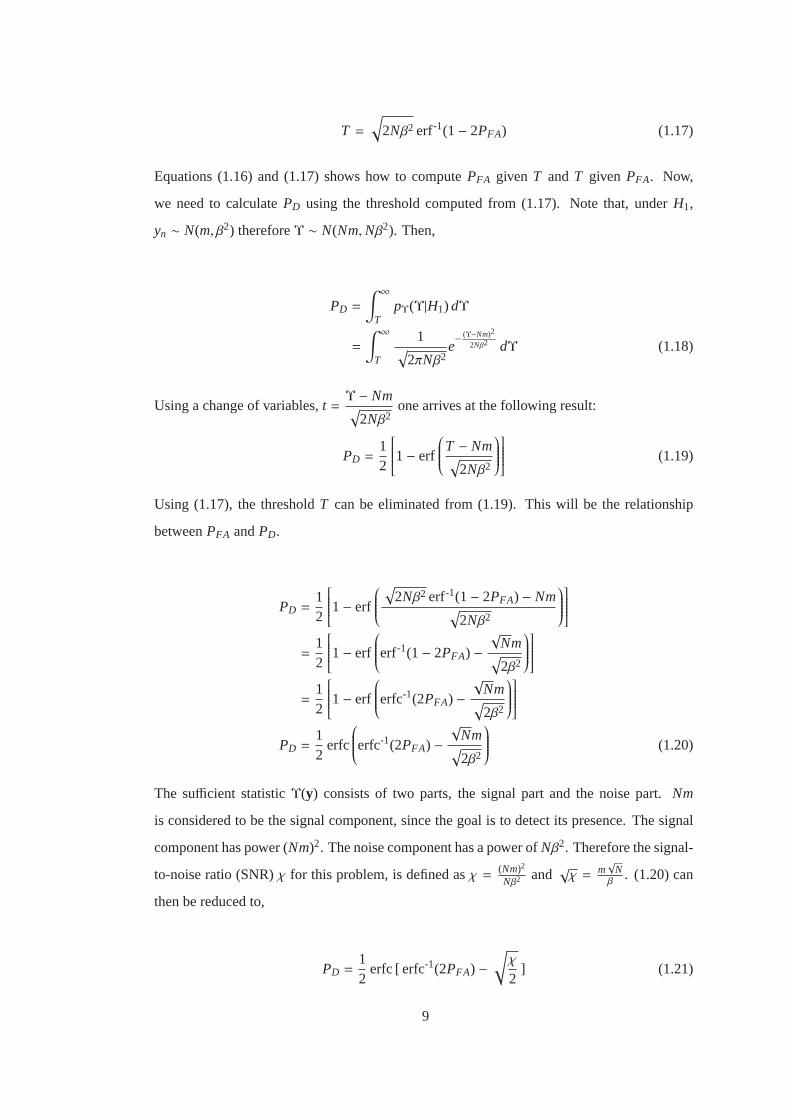
T =√

2Nβ2 erf-1(1− 2PFA) (1.17)

Equations (1.16) and (1.17) shows how to computePFA given T and T given PFA. Now,

we need to calculatePD using the threshold computed from (1.17). Note that, underH1,

yn ∼ N(m, β2) thereforeΥ ∼ N(Nm,Nβ2). Then,

PD =

∫ ∞

TpΥ(Υ|H1) dΥ

=

∫ ∞

T

1√2πNβ2

e− (Υ−Nm)2

2Nβ2 dΥ (1.18)

Using a change of variables,t =Υ − Nm√

2Nβ2one arrives at the following result:

PD =12

1− erf

T − Nm√

2Nβ2

(1.19)

Using (1.17), the thresholdT can be eliminated from (1.19). This will be the relationship

betweenPFA andPD.

PD =12

1− erf

√

2Nβ2 erf-1(1− 2PFA) − Nm√2Nβ2

=12

1− erf

erf-1(1− 2PFA) −√

Nm√2β2

=12

1− erf

erfc-1(2PFA) −√

Nm√2β2

PD =12

erfc

erfc-1(2PFA) −√

Nm√2β2

(1.20)

The sufficient statisticΥ(y) consists of two parts, the signal part and the noise part.Nm

is considered to be the signal component, since the goal is to detect its presence. The signal

component has power (Nm)2. The noise component has a power ofNβ2. Therefore the signal-

to-noise ratio (SNR)χ for this problem, is defined asχ = (Nm)2

Nβ2and√χ = m

√Nβ

. (1.20) can

then be reduced to,

PD =12

erfc [ erfc-1(2PFA) −√χ

2] (1.21)

9

(1.21) is very useful in the sense that one can analytically determine thePD for a givenPFA

and SNR. Also, it can be seen thatPD andPFA must rise or fall together and the only way

to increasePD for a givenPFA is to increase the SNR for such an optimal detector. All these

calculations lead to the following (optimal) detector setup.

y[n]∑N−1

i=0(.)

H1

≷H0

T Detection Decision

Figure 1.1: Detector setup for a known constant in Gaussian noise

1.3.3 Coherent Detection

Even though the Gaussian problem considered so far is useful for introducing and explaining

the major elements of detection such as Neyman-Pearson criteria or the likelihood ratio test,

it is not a very good example for modeling real life situations such as radar or sonar detection.

Most radar systems use coherent detection, which produces complex-valued measurements.

The approach considered so far is valid for real valued data only. Also, the Gaussian approach

does not account for unknown parameters. The target amplitude and noise variance, for ex-

ample, are mostly unknown and must be estimated.

An appropriate model for the noise at the output of a coherent receiver is developed in [4].

The I and Q channels will contain independent, identically distributed zero-mean white Gaus-

sian noise with powerβ2/2. A complex noise process, for which the real and imaginary

parts are independent, identical and zero mean is called acircular symmetric complex normal

distribution. The joint pdf ofN complex samples of this distribution is:

py(y) =1

πN det (Γ)exp{−(y −m)HΓ−1(y −m)} (1.22)

Herem is theN×1 vector of means of the signaly = m+w, Γ is theN×N covariance matrix

of y andΓ = E{yyH} −mmH. Since the noise samples are i.i.d,Γ = β2I N , det{Γ} = β2N and

10

Γ−1 = 1

β2I N . Then, (1.22) reduces to:

py(y) =1

πNβ2Nexp{− 1

β2(y −m)H(y −m)} (1.23)

One can then write the LRT as:

Λ =py(y|H1)

py(y|H0)=

1πNβ2N exp{− 1

β2(y −m)H(y −m)}

1πNβ2N exp{− 1

β2yHy}

= exp{− 1β2

(yHy − yHm −mHy +mHm − yHy)}

= exp{ 1β2

(2 Re{mHy} −mHm)}

lnΛ =1β2

[2 Re{mHy} −mHm]

=2β2

Re{N−1∑

n=0

m ∗ yn}︸ ︷︷ ︸

Matched Filter

− 1β2

N|m|2︸︷︷︸Energy of them vector

(1.24)

(1.24) can be interpreted in the following way. The first term involves a dotproduct of two

complex vectorsm andy. This represents an FIR filtering operation and since the impulse

response of this filter is identical to the signal to be detected underH1, it can be named as a

matched filter. The second term, is obviously the energy of the signalm. Denote this energy

asE = N|m|2.

Obviously, looking at (1.24) one can deduce that the sufficient statisticΥ(y) = Re{mHy}.

Expressing the LRT in terms of sufficient statistic yields:

Υ = Re{mHy}H1

≷H0

β2

2ln (−λ) + E

2= T (1.25)

Now we need to determine the pdf of the sufficient statisticΥ under bothH0 and H1. Let

z = mHy. Sincez is just the sum of independent Gaussian random variables, it will also be

Gaussian. UnderH0, yn is zero-mean noise and so isz. The variance is found from:

11

z = mHy =N−1∑

n=0

mn ∗ yn

var(z) = var(N−1∑

n=0

mn ∗ yn)

=

N−1∑

n=0

var(mn ∗ yn) =N−1∑

n=0

|mn|2 var(yn)︸ ︷︷ ︸β2

= β2N−1∑

n=0

|mn|2

︸ ︷︷ ︸E

= Eβ2 (1.26)

UnderH0, z ∼ N(0, Eβ2). Similarly underH1, z ∼ N(E, Eβ2). We need to find the pdf of

Re{z}. Gaussian noise splits evenly between the real and imaginary parts ofz [3]. Therefore

underH0, Υ ∼ N(0, Eβ2/2) and underH1, Υ ∼ N(E, Eβ2/2). Evaluating thePFA expression,

PFA =

∫ ∞

TpΥ(Υ|H0) dΥ

=

∫ ∞

T

1√2πEβ2/2

e− Υ2

Eβ2 dΥ (1.27)

Making the substitutiont = Υ√Eβ2

, it is clear that

PFA =12

1− erf

T√β2E

(1.28)

T =√β2E erf-1 (1− 2PFA) (1.29)

Repeating the same procedure used before,

PD =12

erfc

erfc-1(2PFA) −

√E

β2

(1.30)

As before,E is the signal energy andβ2 is the signal power. Therefore the SNR,χ = E/β2.

Then,

12

PD =12

erfc(erfc-1(2PFA) − √χ

)(1.31)

We arrive at the same conclusion that SNR must be increased to improve detection perfor-

mance for a given false alarm probability.

1.3.4 Unknown parameters

Up to now, every component of the pdfspΥ(Υ|H0) andpΥ(Υ|H1) were assumed to be known.

In the Gaussian example, the signal meansm and the noise varianceβ2 were assumed to be

known. This is not the case in the real world because these parameters cannot be known per-

fectly. Now consider the case where the magnitude of the returning signalm is known but

the phase is not. Letm = m exp (jθ) where the signal phase,θ can be modeled as a uniform

random variable distributed in [0,2π].

Using theBayes theorem, one can find the pdf of a random variable by conditioning it on

other random variables. For this case,

py(y|Hi) =∫

py(y|Hi, θ)pθ(θ) dθ i = 0,1 (1.32)

Then the following pdfs can be defined:

py(y|H0, θ) =1

πNβ2Nexp [− 1

β2yHy] (1.33)

py(y|H1, θ) =1

πNβ2Nexp[− 1

β2(y − me jθ)H(y − me jθ)] (1.34)

Note thatpy(y|H0) does not depend onθ, so there is no need to use Bayes theorem. (ie:

py(y|H0) = py(y|H0, θ)) For py(y|H1):

py(y|H1, θ) =1

πNβ2Nexp

[− 1β2

(yHy − 2 Re{mHye− jθ} +mHm)]

=1

πNβ2Nexp

[− 1β2

(yHy − 2|mHy| cos (φ − θ) + E)]

(1.35)

13

whereφ is the unknown, but fixed, phase of the inner productmHy. Using,

py(y|H1) =∫

py(y|H1, θ)pθ(θ) dθ we get:

py(y|H1) =1

πNβ2Ne−(yHy+E)/β2 1

2π

∫ 2π

0exp

[ 2β2|mHy| cosθ

′]

dθ′

(1.36)

whereθ′= φ − θ. To evaluate this integral, one needs to use the following definition of the

modified Bessel function of the first kind,I0(x).

I0(x) ,12π

∫ 2π

0ex cosθ dθ (1.37)

Using this result, (1.36) becomes

py(y|H1) =1

πNβ2Ne−(yHy+E)/β2I0

(2|mHy|β2

)(1.38)

The LRT and the log-LRT now become

Λ =py(y|H1)

py(y|H0)=

1πNβ2N e−(yHy+E)/β2I0

(2|mHy|β2

)

1πNβ2N e

(− 1β2

yHy)

= e− Eβ2 I0

(2|mHy|β2

)(1.39)

lnΛ = ln[I0

(2|mHy|β2

)]− E

β2

H1

≷H0

ln (−λ) (1.40)

Alternatively,

ln[I0

(2|mHy|β2

)]

︸ ︷︷ ︸Υ

H1

≷H0

T (1.41)

Using the LRT and (1.41) the signal processing required for optimal detection of a signal

in the presence of unknown phase is determined. One needs to pass the signal through a

14

matched filter, then take its magnitude and apply the nonlinearity ln [I0()]. Because the func-

tion ln [I0()] is a monotonically increasing function, same results can be obtained usingthe

threshold test

|mHy|H1

≷H0

T ′ (1.42)

To establish the performance of this detector, we need to findPFA andPD for the threshold

test explained in (1.42). Letz = mHy. We need to find the distribution of|z| under both

H0 and H1. Under H0, we know mHy ∼ N(0, Eβ2) and the real and imaginary parts of

mHy are independent with varianceEβ2/2. Using |z| =√

zR2 + zI

2 wherezR andzI denote

the real and imaginary parts ofz respectively and both of them areN(0, Eβ2/2). Using the

following property of Rayleigh distribution;R ∼ Rayleigh(σ) is a Rayleigh distribution ifR =√

X2 + Y2 whereX ∼ N(0, σ2) andY ∼ N(0, σ2) are two independent normal distributions.

SincezR andzI are two independent zero-mean normal distributions,|z| is Rayleigh distributed

with the parameterσ2 = Eβ2/2. Then:

pz(z|H0) =z

Eβ2/2e(−z2/Eβ2) (1.43)

The false alarm probability is

PFA =

∫ ∞

Tpz(z|H0) dz

=

∫ ∞

T

2z

Eβ2e(−z2/Eβ2) dz

The substitutiont = z2

Eβ2, dt = 2zdz

Eβ2leads the following results,

PFA =

∫ ∞

T2

Eβ2

e−t dt = exp (−T 2

Eβ2) (1.44)

T =√−Eβ2 ln PFA (1.45)

The threshold for a given false alarm probability can be computed from (1.44) and (1.45). Let

us calculate thePD for this given threshold. UnderH1 , mHy ∼ N(E, Eβ2). Again let z =

15

mHy. SinceE is real valued,zR ∼ N(E, Eβ2/2) andzI ∼ N(0, Eβ2/2). Using the following

property of Rician distribution:R ∼ Rice(ν, σ) has a Rice distribution ifR =√

X2 + Y2

whereX ∼ N(ν cosθ, σ2) andY ∼ N(ν sinθ, σ2) are statistically independent normal random

variables andθ is any real number. In our case,ν = E , θ = 0 andσ2 = Eβ2/2.

pz(z|H1) =2z

Eβ2exp

[− (

z2 + E2

Eβ2)]I0(

2z

β2) (1.46)

The required integral isPD =∫ ∞

Tpz(z|H1) dz. The required integral can be reduced to the

following normal form which is calledMarcum’s Q function.

QM(α, γ) =∫ ∞

γ

t exp[− 1

2(t2 + α2)

]I0(αt) dt (1.47)

Letting t = z√Eβ2/2

andα =√

2Eβ

gives the following result:

PD = QM

(√2E

β2,

√2T 2

Eβ2

)(1.48)

Using the definition of SNR,χ = E/β2 andT =√−Eβ2 ln PFA one arrives at:

PD = QM(√

2χ,√−2 ln PFA) (1.49)

16

All these calculations lead to the following detector setup.

y[n]Matched Filter

mHy

Magnitude|.|

H1

≷H0

T Detection Decision

Figure 1.2: Detector setup for a known constant with unknown phase in Gaussian noise

1.3.5 Radar Signal Detection

In a realistic radar scenario, the amplitude and phase of the returning signal, the time of arrival

and the Doppler shift are unknown. To account for these unknown parameters, some more

signal processing techniques must be used. There are many methods used to improve detec-

tion performance under such situations such as coherent integration, non-coherent integration,

binary integration etc. Also targets can be non-fluctuating (ie: constant) orfluctuating. Here

only the case of non-fluctuating targets will be explained.

Let yn be the individual data samples where underH0, yn = wn and underH1, yn = m + wn.

Herem = m exp jθ for some real amplitude ˜m and random phaseθ. UnderH0, the pdf of

zn = |yn| is the Rayleigh pdf:

pzn(zn|H0) =2zn

β2e(−zn

2/β2) (1.50)

UnderH1, zn has the Rician pdf:

pzn(zn|H1) =2zn

β2e−(

z2n+m2

β2)I0(

2mzn

β2) (1.51)

The joint pdf ofN-samples ofzn is:

17

pz(z|H0) =N−1∏

n=0

2zn

β2e(−zn

2/β2) (1.52)

pz(z|H1) =N−1∏

n=0

2zn

β2e−(

z2n+m2

β2)I0(

2mzn

β2) (1.53)

The LRT and the log-LRT can be written as:

Λ =pz(z|H1)pz(z|H0)

=

∏N−1n=0

2znβ2

e−(

z2n+m2

β2)I0(2mzn

β2)

∏N−1n=0

2znβ2

e(−zn2/β2)

=

N−1∏

n=0

exp (− m2

β2)I0(

2mzn

β2)

= e−m2/β2N−1∑

n=0

I0(2mzn

β2) (1.54)

lnΛ = − m2

β2+

N−1∑

n=0

ln[I0(

2mzn

β2)]

(1.55)

In sufficient statistic form,

ln[I0(

2mzn

β2)] H1

≷H0

ln (−λ) + m2

β2= T (1.56)

Using the approximation:

ln [I0(x)] ≈ x2

4, ln [I0(

2mzn

β2)] ≈ 4m2zn

2

β4

The detection test then becomes:

N−1∑

n=0

m2zn2

β4

H1

≷H0

T

N−1∑

n=0

zn2

︸ ︷︷ ︸Υ

H1

≷H0

T ′ (1.57)

18

Looking at (1.57) the sufficient statisticΥ turns out to be the sum of the magnitude squares

of the individual data samples. The performance of this detector should now be calculated.

Figure (1.3) shows the proposed detector setup and the correspondingpdfs underH0.

yn|.|β (.)2

∑N−1

n=0(.)

H1

≷H0

T

z′n

Rayleigh

rn

Exponential

z

Erlang

Figure 1.3: Detector setup for nonfluctuating targets and correspondingpdfs underH0

We know thatyn is normal with zero mean and varianceβ2 distributed evenly between its

independent real and imaginary parts. Its magnitude,|yn|, is Rayleigh distributed,|yn| ∼

Rayleigh(√β2/2). Sincez′n = |yn|/β, z′n ∼ Rayleigh(1/

√2). Using the fact that, forY ∼

Rayleigh(σ), X ∼ Exponential(λ) if X = Y2

2λσ2 . Hereσ2 = 1/2 , so λ = 1 and rn ∼

Exponential(1). Ifxi ∼ Exponential(λ) andY =∑N−1

i=0 xi thenY ∼ Gamma(N,1/λ). Here

λ = 1 soz ∼ Gamma(N,1), Gamma distribution with integer shape parameter is also called

the Erlang distribution. So the pdf ofz is:

fz(z|H0) =zN−1e−z

(N − 1)!(1.58)

To find PFA one needs to consider the integral:

PFA =

∫ ∞

T

zN−1e−z

(N − 1)!dz (1.59)

For the case ofN = 1 (single sample) (1.59) reduces to:

PFA = e−T (1.60)

T = − ln PFA (1.61)

19

The detection probability for this case and whenN , 1 is quite complicated and can be found

in [4]. When the normalization (division byβ in Figure (1.3)) is not done,T = −β2 ln PFA

andPFA = e−T/β2. The square law detector for a single sample uses these expressions to set

the threshold for a given false alarm probability and known noise variance.

20

CHAPTER 2

CONSTANT FALSE ALARM RATE DETECTION

Up to this point, we have assumed that the interference level (ie:β) is known and constant,

thus allowing one to set the threshold for a desired false alarm probability. However, in real

life applications that is rarely the case. In practice, the interference levelsare rarely known and

they are not constant. To combat these difficulties, a set of adaptive methods jointly known

asConstant False Alarm Rate (CFAR) methods are used. These methods provide predictable

detection performance and false alarm probability under real life scenarios.

2.1 Case of Unknown Interference Power

As noted earlier, the expressions for false alarm probability and the required threshold are

as followsT = −β2 ln PFA and PFA = e−T/β2. Assume that the threshold is preset using

an estimated interference powerβ0 to satisfy a false alarm probabilityPFA0, but the actual

interference power isβ2. Let us calculate the increase in the false alarm probability.

PFA = exp(β2

0 ln PFA0

β2

)= exp

(ln P

β20/β2

FA0

)

= Pβ20/β

2

FA0 (2.1)

(2.1) shows that even a small increase of 2dB can cause an increase inPFA of 1.5 to 3 orders

of magnitude. This is highly undesirable and shows that the actual interference powerβ2 must

be estimated from the data in real time. This estimate will then be used to set the threshold.

A detector that can maintain a constant false alarm rate regardless of the interference power,

is called a constant false alarm rate (CFAR) processor.

21

2.2 Types of CFAR Processors

General scheme of a CFAR detector is shown in Figure 2.1. The threshold adjustment for a

specific resolution cell is based on the signal levels around it. There are many variations and

modifications to this general scheme.

Figure 2.1: General CFAR Detector scheme

2.2.1 Cell Averaging CFAR

Previously, it was shown that for the square law detector, each cellxi has an exponential pdf

with the parameterβ2. It can easily be shown that the maximum likelihood (ML) estimate of

β2 for a vectorx of N such samples is just the average of the available samples. [4].

β2 =1N

N∑

i=1

xi (2.2)

The threshold is then set as a multiple of estimated interference power.

T = αβ2 (2.3)

Since the interference power and therefore the threshold are estimated from the average power

in the cells around the test cell, this approach is called cell-averaging CFAR.To find α, one

needs to consider the effect of estimating noise power over a finite number of cells, rather than

22

knowing it exactly.

The estimated threshold can be written as

T =α

N

N∑

i=1

xi (2.4)

Let y =∑N

i=1 xi. We know that the sum ofN independent identically distributed exponential

random variables with rateλ has the distribution Gamma(N,1/λ). Then pdf ofy is the Erlang

density

py(y) =1β2N

yN−1

(N − 1)!e−y/β2 (2.5)

SinceT = (α/N)y, the pdf ofT is (for T > 0)

pT (T ) =( N

αβ2

)N T N−1

(N − 1)!e−NT/αβ2 (2.6)

For the thresholdT , PFA = e−T/β2. The expected value ofPFA is now

PFA =

∫ ∞

−∞e−T/β2 pT (T ) dT

=

( N

αβ2

)N 1(N − 1)!

∫ ∞

0T N−1e−T/β2e−NT/αβ2 dT

=

( N

αβ2

)N 1(N − 1)!

∫ ∞

0T N−1e−[(N/α)+1]T/β2 dT (2.7)

Using the fact that

∫ ∞

0xne−ax dx =

n!an+1

for integern (2.8)

one can compute (2.7) as

PFA =

(1+α

N

)−N(2.9)

23

and the threshold multiplier for a givenPFA as

α = N(P−1/NFA − 1) (2.10)

Equations (2.9) and (2.10) can be used to set the threshold for a fixed false alarm probability.

It also shows that since the false alarm probability does not depend on theactual interference

power, this detector exhibits CFAR behavior. The average detection probability is found as

[4].

PD =

(1+

α

N(1+ χ)

)−N(2.11)

whereχ is the SNR.

xi

Leading

Window

Guard

Cells

Guard

Cells

Lagging

WindowRange

Figure 2.2: CFAR reference window.xi is the cell under test (CUT)

Figure(2.2) shows the reference window arrangement for a one-dimensional data vector of

range (or time) cells. The gray cells are called thereference cells and represent the data from

ranges nearer and farther from the cell under test (xi). These cells are averaged to find the

estimate of the noise power. The dotted cells are calledguard cells and are excluded from the

averaging operation. This is due to the fact that the cells immediately adjacent toxi would

contain both interference and target energy and do not represent theinterference alone. If

these cells were included in the averaging operation, the estimate ofβ2 would be too high.

This, in turn, causes the detection threshold to be too high, lowering thePFA andPD. Obvi-

ously, this is not desired. The combined window of guard cells, reference cells and the cell

under test (CUT) is called asCFAR window.

24

Since the threshold is estimated from a finite number ofN samples rather than exactly known,

the threshold is usually higher than the ideal one. This is necessary to compensate for the

unknown interference power and to guarantee the desiredPFA. Since the threshold multiplier

is higher than ideal, this means that to achieve a specifiedPD for a givenPFA a higher SNR is

necessary than would be were the noise power known exactly. This increase in SNR is called

theCFAR loss. To quantify this CFAR loss, plug (2.10) into (2.11)

PD =

(1+

N(P−1/NFA − 1)

N(1+ χ)

)−N

(2.12)

If (2.12) is solved for the required SNR for a givenPD andPFA we get

χN =(PD/PFA)1/N − 1

1− P1/ND

(2.13)

whereχN is a function of the number of cells averaged. It can be shown that ([4],[6]) that as

N → ∞, the SNRχ∞ is

χ∞ =ln (PFA/PD)

ln (PD)(2.14)

Then, the CFAR loss is defined as

LCFAR =χN

χ∞(2.15)

It has been reported that for small (N < 20) reference windows, the CFAR loss can be several

dB [4]. High CFAR losses does not permit the use of values ofN less than 10.

CA CFAR algorithms have some drawbacks. First of all, the threshold value increases in the

vicinity of the target. When two or more targets are present and one target isin the test cell

while another target is in the reference cell, the threshold value will increase. The target in the

reference window can ’mask’ the the target in the test cell because of thisincreased threshold,

this effect is called target masking. Also, for targets that accompany many range cells, the

reference cell and the test cell might both contain targets and this might cause the target to

25

mask ’itself’. This is called self masking. In addition to masking effects, CA CFAR suffers

from false alarms atclutter edges. Clutter edges are the boundaries between two clutter re-

gions having different reflectivities. These edges can cause false alarms at the edge and allow

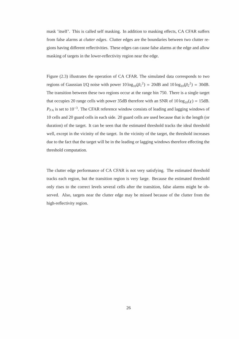
masking of targets in the lower-reflectivity region near the edge.

Figure (2.3) illustrates the operation of CA CFAR. The simulated data corresponds to two

regions of Gaussian I/Q noise with power 10 log10(β12) = 20dB and 10 log10(β2

2) = 30dB.

The transition between these two regions occur at the range bin 750. There is a single target

that occupies 20 range cells with power 35dB therefore with an SNR of 10 log10(χ) = 15dB.

PFA is set to 10−3. The CFAR reference window consists of leading and lagging windows of

10 cells and 20 guard cells in each side. 20 guard cells are used becausethat is the length (or

duration) of the target. It can be seen that the estimated threshold tracks theideal threshold

well, except in the vicinity of the target. In the vicinity of the target, the thresholdincreases

due to the fact that the target will be in the leading or lagging windows therefore effecting the

threshold computation.

The clutter edge performance of CA CFAR is not very satisfying. The estimated threshold

tracks each region, but the transition region is very large. Because the estimated threshold

only rises to the correct levels several cells after the transition, false alarms might be ob-

served. Also, targets near the clutter edge may be missed because of the clutter from the

high-reflectivity region.

26

0 100 200 300 400 500 600 700 800 900 100020

25

30

35

40

45

50CA CFAR

Range Cell

Pow

er(d

B)

Target

Clutter Edge

SNR=20dB

PF A = 10−2

β2

1=20dB

β2

2=30dB

InputCA CFARIdeal Threshold

Figure 2.3: CA CFAR threshold behavior and clutter edge performance

The main advantage of CA CFAR is that it is simple to perform and does not require a lot

of computing power. Nonetheless, non homogeneous clutter and the presence of interfering

targets have led to the development of some extensions to the CA CFAR concept. These ex-

tensions are designed to combat one or more of the shortcomings of the CA CFAR algorithm.

2.2.2 Smallest-of-Cell-Averaging CFAR

The smallest-of-cell-averaging CFAR (SOCA CFAR) is intended to combat themasking ef-

fects caused by interfering targets among the CFAR reference cells. Letthe estimate of the

noise power in the leading window beβ21 and the lagging window beβ2

2. The SOCA CFAR

approach estimates the threshold by taking the minimum of these estimates.

T = αso min (β12, β2

2) (2.16)

If an interfering target is present in one of the reference windows, its threshold estimate will

27

0 100 200 300 400 500 600 700 800 900 100020

25

30

35

40

45

50SOCA CFAR

Range Cell

Pow

er(d

B)

Target Clutter Edge

SNR=15dB

PF A = 10−3

β2

1=20dB

β2

2=30dB

InputCA CFARIdeal Threshold

Figure 2.4: SOCA CFAR threshold behavior and clutter edge performance

increase. Because of the minimum operator, the other reference cell will be chosen and detec-

tion will successfully be performed. Since the threshold is estimated usingN/2 cells instead

of N cells, the threshold multiplier will have to change. It is shown that the requiredmultiplier

can be found from solving (2.17) iteratively [7]

PFA/2 =(2+αso

N/2

)−N/2[ N/2−1∑

k=0

(N/2− 1+ k

k

)(2+αso

N/2

)−k](2.17)

Figure (2.4) shows the SOCA CFAR behavior and clutter edge performance. Unlike CA

CFAR, the threshold does not increase in the vicinity of the target. This is dueto the use

of minimum operator. When the target is in the lagging window, the leading windowhas a

smaller estimated threshold and therefore the leading window is chosen by the minimum op-

erator. Similarly, when the target is in the leading window, the lagging window has a smaller

estimated threshold and therefore the lagging window is chosen. This allows for the correct

28

setting of threshold. This also allows for combating the effects of multiple targets and self

masking. Using SOCA CFAR, detection of closely spaced targets is possible.

The main failing point of SOCA CFAR algorithm is seen in clutter edges. When theCFAR

window crosses the clutter edge, there will be a region where the test cell isin the higher

interference region and the leading window is filled mostly with the lower interference region.

The minimum operator makes sure that the threshold is estimated using the lower interference

power and therefore many false alarms are seen during the transition region.

2.2.3 Greater-of-cell-averaging CFAR

For environments where interfering or closely-spaced targets are unlikely but the clutter is

highly non homogeneous and clutter edge false alarms are very important, another CFAR ap-

proach is developed. In this case, the greater-of-cell-averaging CFAR (GOCA CFAR) is used.

Just like the previous method, GOCA CFAR uses the threshold estimate shown in(2.18)

T = αGO max (β12, β2

2) (2.18)

Similar to the SOCA case, the GOCA multiplier is found from [7]

PFA/2 =(1+αGO

N/2

)−N/2−

(2+αGO

N/2

)−N/2×

[ N/2−1∑

k=0

(N/2− 1+ k

k

)(2+αGO

N/2

)−k]

The operation of GOCA CFAR can be seen in Fig.(2.5). Not surprisingly, the maximum oper-

ator successfully avoids the false alarms at the clutter edge. However, thethreshold increases

abruptly in the vicinity of the target and this increase is larger than that of CA CFAR. This

means that the GOCA CFAR algorithm is more vulnerable target masking and selfmasking

effects. If there is more than one target present, the stronger targets may maskthe weaker

targets. The GOCA CFAR may also miss targets near the clutter edge due to the transition

region.

29

0 100 200 300 400 500 600 700 800 900 100020

25

30

35

40

45

50GOCA CFAR

Range Cell

Pow

er(d

B)

Target

Clutter Edge

SNR=15dB

PF A = 10−3

β2

1=20dB

β2

2=30dB

InputGOCA CFARIdeal Threshold

Figure 2.5: GOCA CFAR threshold behavior and clutter edge performance

2.2.4 Censored or Trimmed mean CFAR

Another way to combat with interfering targets and target masking problem is tomake use

of the censored or trimmed mean CFAR ([8], [9]). In this approach, theNC reference cells

(NC < N) having the highest power are discarded and the threshold is estimated using the re-

mainingN − NC cells. Such detectors are called asCensored Mean Level Detector (CMLD).

Censoring the cells having the lowest power is also possible and this approach is useful in

reducing bias problems when the noise has a spectral slope [10]. However, here we are con-

cerned with detection robustness in multiple target environments and will therefore concen-

trate on CMLDs with censoring applied to cells having higher power since when an interferer

is present in the noise reference samples, that sample is expected to have ahigh power. The

CMLD detector uses the threshold estimate shown in (2.19)

T = αCMLD

N−NC∑

j=1

x( j) (2.19)

30

whereαCMLD is the threshold multiplier,NC is the number of censored cells and the sequence

{x(1), x(2), . . . , x(n)} is the ordered sequence of reference cells such thatx(1) ≤ x(2) ≤ . . . ≤

x(k) ≤ . . . ≤ x(n). The threshold multiplier is found from [11]

PFA = M ×( 11+ αCMLD

)N−NC−1

(2.20)

where

M =N!

NC!(N − NC − 1)!(N − NC)×

NC∑

j=0

(NC

j

)(−1)NC− j

N− jN−NC

+ αCMLD

(2.21)

This process of censoring will eliminate the elevating effect of interfering targets on the

threshold estimate. The choice ofNC requires the knowledge of how many interfering tar-

gets are expected. It is noted that typically half to a quarter of the cells are discarded [12].

The censoring method can be combined with any of the CA, SOCA or GOCA techniques

as in [13]. In censored CA CFAR (CMLD), theNC cells having the highest power are dis-

carded from both the leading and lagging windows, then conventional CA method is used as

in (2.19). The censored GOCA and censored SOCA CFAR methods are also reasonable.

The operation of CMLD can be seen in Fig.(2.6). There is an increase of the threshold in the

vicinity of the target however it is much less than the increase in standard CA CFAR. This

means this method can tolerate interfering targets and masking effects. The clutter edge per-

formance of CMLD is worse than CA CFAR and SOCA CFAR [11]. The main disadvantage

of censored CFAR methods is that they require implementation of a logic to rank and order

the cells.N number of cells must be ordered for every reference window and this means in-

creased algorithm complexity and computational power. Alternate equations for PD andPFA

can be found in [8].

2.2.5 Order Statistic CFAR

The censored CFAR approach has introduced the idea of ordering to theCFAR concept. A

new class of CFAR detectors, namelyrank-based or order-statistic CFARs (OS CFAR), then

31

0 100 200 300 400 500 600 700 800 900 100020

25

30

35

40

45

50Censored CFAR

Range Cell

Pow

er(d

B)

Target

Clutter Edge

SNR=20dB

PF A = 10−3

β2

1=20dB

β2

2=30dB

N =10 cells are censored

InputCensored CFARIdeal Threshold

Figure 2.6: CMLD threshold behavior and clutter edge performance

emerged. The primary purpose of this type of detectors is to combat multiple targets and

masking effects. The sliding window structure of CA CFAR is still used but guard cells

are much less important because the averaging operator is not used to estimate the interfer-

ence level. Instead, OS CFAR rank orders the reference window data samples and chooses

only one element of the ordered list as a representative of the threshold level. The samples

are ordered to form a new sequence in ascending numerical order{x(1), x(2), . . . , x(n)} where

x(1) ≤ x(2) ≤ . . . ≤ x(k) ≤ . . . ≤ x(n). The kth element of the ordered list (x(k)) is called

the kth order statistic. In OS CFAR, thekth order statistic is used as a representative of the

interference level and the threshold is set as a multiple of this value

T = αOS x(k) (2.22)

Note that the threshold is estimated using only one sample, instead of an average of all data

samples. However, all the data samples are required to determine which will bethekth largest,

32

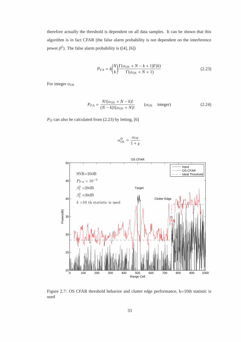
therefore actually the threshold is dependent on all data samples. It can be shown that this

algorithm is in fact CFAR (the false alarm probability is not dependent on theinterference

powerβ2). The false alarm probability is ([4], [6])

PFA = k

(Nk

)Γ(αOS + N − k + 1)Γ(k)Γ(αOS + N + 1)

(2.23)

For integerαOS

PFA =N!(αOS + N − k)!

(N − k)!(αOS + N)!(αOS integer) (2.24)

PD can also be calculated from (2.23) by letting, [6]

αDOS =

αOS

1+ χ

0 100 200 300 400 500 600 700 800 900 100020

25

30

35

40

45

50OS CFAR

Range Cell

Pow

er(d

B)

Target

Clutter Edge

SNR=20dB

PF A = 10−3

β2

1=20dB

β2

2=30dB

k =10 th statistic is used

InputOS CFARIdeal Threshold

Figure 2.7: OS CFAR threshold behavior and clutter edge performance, k=10th statistic isused

33

Fig(2.7) shows the operation of OS CFAR and its clutter edge performance whenN = 20 and

k = 10. There is small increase in the threshold after the reference cell has passed the target

window, the reason for this is the target is long and occupies more thanN − k reference cells.

However, this increase is not very large and can be tolerated. Guard cells are less important

in OS CFAR, since the rank ordering process will not be affected by targets outside the test

cell. The clutter edge performance of OS CFAR is given in [14]. Typicallyk is on the order of

3N/4 [12]. OS CFAR method is completely insensitive to masking of closely spaced targets,

however it requires the implementation of a sorting logic and therefore the computational

load for this algorithm is high. OS CFAR losses are lower than CA CFAR lossesin the case

of interfering targets [15]. Some additional results on the performance ofOS CFAR in non

homogeneous clutter and Weibull clutter are available in [16].

2.2.6 Variability Index CFAR

The Variability Index CFAR (VI CFAR) utilizes a background estimation algorithm which is

a mixture of the CA CFAR, SOCA CFAR and GOCA CFAR. VI CFAR uses a statistical test

to dynamically select the particular group of reference cells to use to estimate the threshold.

This particular group can be; leading half of reference cells, lagging half of reference cells, or

all of the reference cells. This dynamical selection provides the VI CFAR algorithm with low

loss CFAR performance in a homogeneous environment and also robust performance in non

homogeneous environments filled with multiple targets and clutter edges. ([17],[18])

The block diagram of VI CFAR can be seen in Fig(2.8). The VI is a second-order statistic

closely related to an estimate of the shape parameter of a probability distribution.It closely

resembles the coefficient of variation. It is defined as

VI = 1+σ2

µ2(2.25)

whereµ is the estimated mean and ˆσ2 is the estimated variance of the split window. Then, the

VI is calculated for each split window and compared with a thresholdKVI to decide if the cells

with which the VI is computed are from a homogeneous or non homogeneous environment.

The following logical test is used

34

Figure 2.8: VI CFAR Block Diagram

VI ≤ KVI =⇒ Nonvariable

VI > KVI =⇒ variable (2.26)

The mean ratio (MR) is defined as the ratio of the estimated mean values of the leading and

lagging reference window cells.

MR =XA

XB=

∑

i∈AXi/

∑

i∈B

Xi (2.27)

The MR is compared with a thresholdKMR to decide if the populations have the same means

or different means. The following logical test is used

MR < KMR−1 or MR > KMR =⇒ Different means

Otherwise=⇒ Same means (2.28)

After the VI and MR has been calculated for each split reference window, Table (2.1) is used

to set the adaptive threshold.

The VI CFAR is less complex than the OS CFAR and offers betterPFA performance in a

35

Leading Lagging EquivalentWindow Window Different VI-CFAR CFARVariable? Variable? Means? Threshold method

No No No CN .ΣAB CA CFARNo No Yes CN/2.max(ΣA,ΣB) GOCA CFARYes No - CN/2.ΣB CA CFARNo Yes - CN/2.ΣA CA CFARYes Yes - CN/2.min(ΣA,ΣB) SOCA CFAR

Table 2.1: VI CFAR adaptive threshold selection

clutter edge environment and similarPD performance in a multiple target environment. The

selection of the parametersKMR andKVI and performance results of the VI CFAR algorithm

can be found in [18].

2.2.7 Switching CFAR

A threshold is set using the magnitude of the cell under test. Then, the cells in the reference

window are put into two groups, those above the said threshold and those below them. If the

number of cells that are below the threshold is larger than someNt, all N cells are used in a

cell averaging calculation. If the number of low amplitude cells is less thanNt, the threshold

is set using only the low amplitude cells. This method causes reduced CFAR losses compared

to other methods and somewhat improved clutter-edge performance. The need for sorting is

avoided. The clutter edge performance is not so good, it is worse than VI-CFAR in terms of

false alarms in clutter edges. Equations forPD andPFA can be found in [19].

2.2.8 Log CFAR

To combat target masking effects, one can use a log detector (instead of a linear or square

law detector) and then can apply the conventional CA CFAR methods to the logarithm of the

samples. There is no simple closed form for determining the relationship between an average

of the log-detected data and the interference powerβ2. However, motivated by the form of

(2.3) one can write

Tlog =1N

N∑

i=1

10 log10(xi) + αlog (2.29)

36

whereαlog is the threshold factor to ensure the designed false alarm probability. The log

CFAR has the ability to operate over a large dynamic range. Also it is less vulnerable to

target masking effects. Interfering targets in the reference window cannot raise the threshold

too greatly because of the log operator. Unfortunately, log CFAR shows poor performance at

clutter edges and has an increased vulnerability to false alarms near clutter edges.

0 100 200 300 400 500 600 700 800 900 100020

25

30

35

40

45

50log CFAR

Range Cell

Pow

er(d

B)

Target

Clutter Edge

SNR=20dB

PF A = 10−3

10 log10

β2

1=20dB

10 log10

β2

2=30dB

Inputlog CFARIdeal Threshold

Figure 2.9: log CFAR threshold behavior and clutter edge performance

Fig.(2.9) shows the thresholds estimated by log CFAR method. Here the multiplierαlog is

found from [4] and [20].αlog = 11.85 dB for N = 20 reference cells andPFA = 10−3. The

increase in the threshold around the vicinity of the target still exists, but compared to the

performance of CA CFAR or GOCA CFAR, this increase is more tolerable. This allows for

easy detection of closely spaced targets and prevention of masking effects. The clutter edge

performance of log CFAR is seen to be poor, because false alarms can occur at clutter edges.

The CFAR loss of log CFAR is larger than that of CA CFAR and the use of log detector

increases the required CFAR window size by about 65 percent [21].

37

2.2.9 Adaptive CFAR

These type of algorithms are constructed to increase CFAR performance innon homogeneous

clutter. Typically, a statistical test is made to determine if the reference cells span one or two

clutter fields. This information is then used to select if SOCA, GOCA or CA CFARap-

proaches will be used. A basic approach is described by [22]. This approach first assumes

that the reference cells span two clutter fields and tries to find the point at which the statistics

change,M, whereM < N. M is found by maximizing the following equation for all possible

M whereM ∈ (1 : N)

LM = −[M ln β21(M) − (N − M) ln β2

2(M)] (2.30)

whereβ21(M) is the sample mean in the first clutter region whereM is assumed to be the tran-

sition point andβ22(M) is the sample mean in the second region spanning the remainingN −M

cells. Once thisM is identified, the cell under test is also known to be in the first or second

clutter region. If the cell under test is in the lower clutter region, the threshold is set using

cells in the lower clutter region only. If the cell under test is in the higher clutterregion, the

threshold is set using cells in the higher clutter region. This prevents excessive false alarms

caused by comparing the cell to the threshold estimated using wrong part of the clutter region.

The procedure above does not account for the possibility that the clutteris uniform. To ac-

count for this possibility, another statistical test can be conducted. AssumeM = 0 and cal-

culate the likelihood shown in (2.30),L0 = −N ln β2, and compare this to the likelihood

computed before. IfL0 > LM the clutter is assumed to be uniform and standard CA CFAR

procedure is applied. The main advantage of this method is that it has great performance at

clutter edges (optimal in Gaussian clutter, [22]). However, it requires additional operations to

determine the changing pointM, therefore increasing the required computational power. Also

if M is estimated incorrectly,PFA increases. Fig.(2.10) shows the operation of this method.

The exceptional clutter edge performance should be noted. The detectionperformance is sim-

ilar to that of CA CFAR.

38

0 100 200 300 400 500 600 700 800 900 100020

25

30

35

40

45

50Adaptive CFAR

Range Cell

Pow

er(d

B)

Target

Clutter Edge

SNR=20dB

PF A = 10−3

10 log10

β2

1=20dB

10 log10

β2

2=30dB

InputAdaptive CFARIdeal Threshold

Figure 2.10: Adaptive CFAR threshold behaviour and clutter edge performance

2.2.10 Clutter Map CFAR

Clutter mapping is a technique used for detection of slowly moving or stationary targets when

the Doppler shift of the target is very close to zero. The threshold for each range cell is

computed as a multiple of the measured clutter in that same cell. The clutter measurement is

updated as follows:

y[n] = γy[n − 1] + (1− γ)x[n] (2.31)

wherey[n] is the estimated clutter reflectivity andx[n] is the currently measured clutter sam-

ple, both at timen. The factorγ controls the weight of the current measured sample compared

to the previous measured samples. This factor can be changed on real time ifnecessary. The

threshold is then set as

39

T [n] = αy[n − 1] (2.32)

It can be seen from (2.32) that the thresholdT [n] depends on the samples from the previous

scan. The reason the current data are not included is, if the current data contains a target, the

clutter measurement would be distorted and the threshold would be raised too high, therefore

creating a self masking effect. The first order difference equation (2.31) corresponds to an IIR

filter and the outputy[n] can be written as

y[n] = (1− γ)∞∑

m=0

γmx[n − m] (2.33)

AveragePFA andPD equations are derived in [23] for a clutter map CFAR approach using

multiple scans. The basic CA and OS approaches can be combined with clutter mapping

techniques to fit the operational needs ([24],[25]).

2.2.11 Other CFAR types

There are other CFAR types such as the two-parameter CFAR which worksfor log-normal

or Weibull pdf ([26], [27] and [28]). The distribution free CFAR [29]is a method in which

no specific form of the pdf of the interference is assumed. For a system operating in a clutter

limited environment, a threshold setting algorithm based on a particular pdf may produce very

large errors when actually another interference pdf is present. This is why distribution free

CFAR methods are important. Also, the combination of various types of CFAR methods is

possible and are presented in literature frequently. ([30], [31], [32], [33] and [34]).

40

CHAPTER 3

CFAR DETECTION USING IIR FILTERS

Motivated by the fact that all CFAR processors use some kind of averaging and windowing,

one can propose a structure similar to that of Clutter Map CFAR. Instead of using a simple

averaging FIR filter, we can use a weighted IIR filter to calculate a weighted moving average

which is still a good estimate of the noise background. The ”exponential smoothing filter”

will be used here which is shown in (2.31) and (2.32). This is different from Clutter Map

CFAR shown in 2.2.10. In clutter map CFAR, the threshold estimate is formed fromdifferent

scans of the same range cell. In the IIR filter approach,x[n] represents the cells in time (or

range) but from the same scan. The detector structure using the IIR filteris shown in Fig.(3.1).

Here the threshold is estimated by filtering the range cells using an IIR filter andthen thresh-

old comparison is made.

x[n] DFT |.|2H1

≷H0

T

IIR Filter

b

y[n]

z[n]

Figure 3.1: The IIR Filter Detector

41

Here the structure of the IIR filter is:

y[n] = γy[n − 1] + (1− γ)z[n]

y[n] = (1− γ)∞∑

m=0

γmz[n − m]

T [n] = αy[n − 1]

whereT [n] is the estimated threshold at timen andz[n] is the magnitude squared DFT bin at

time n. Figure 3.2 shows a block diagram implementation of such a system. This systemis

named as IIR CFAR method.

z[n]y[n] y[n− 1] αy[n− 1]

1− γ

γ

αz−1

ComparatorDetection decision

Figure 3.2: Detection using an IIR Filter

To find the parameterγ, we make the following analysis. We are trying to estimate the param-

eterβ2 and we know that the optimum estimator [35] (for the homogeneous case, Gaussian

interference and signal-free reference cells) is the average,1N

∑Ni=1 zi . Let us call the optimum

estimator as estimator 1, orE1 and let the IIR filter estimator beE2. We will try to select ap-

propriateγ so that these two estimators achieve the same (or close) results. Let mean(z) = µz

and var(z) = σ2z (both can be found from properties of DFT operator but has no significance

here).

42

mean(E1) = mean(1N

N∑

i=1

zi) =1N

N∑

i=1

mean(zi) = µz

mean(E2) = mean{(1− γ)

∞∑

m=0

γmz[n − m]}

= (1− γ)∞∑

m=0

γmµz = µz

Both E1 andE2 are unbiased estimators, independent ofγ. Let us look at the variances ofE1

andE2.

var(E1) = var(1N

N∑

i=1

zi) =1

N2var(

N∑

i=1

zi) =1

N2

N∑

i=1

σ2z =

1Nσ2

z (3.1)

var(E2) = var{(1− γ)

∞∑

m=0

γmz[n − m]}

= (1− γ)2var{ ∞∑

m=0

γmz[n − m]}

= (1− γ)2∞∑

m=0

γ2mσ2z

= σ2z (1− γ)2

∞∑

m=0

γ2m

= σ2z(1− γ)2

1− γ2

var(E2) =1− γ1+ γ

σ2z (3.2)

Equate var(E1) and var(E2) to obtain

1N=

1− γ1+ γ

leaveγ alone to get

γ =N − 1N + 1

(3.3)

(3.3) can be used to select appropriateγ to ’mimic’ cell averaging behavior of N cells. Since

this filter is meant to average out the samples, the threshold multiplierα can be set the same

43

way as in CA CFAR. However, from the literature it can be seen thatαiir , αca. The threshold

multiplier can be found from the following formulas from [23].

PFA =1

∏Mm=0 [1 + α(1− γ)γm]

M → ∞ (3.4)

PD =1

∏Mm=0 [1 + αD(1− γ)γm]

M → ∞ (3.5)

where

αD =α

1+ χ(3.6)

From [36] a faster converging equation can be found.

PFA =1

1+∑M

m=0∏m

k=0α(1−γ)γk

1−γk+1

M → ∞ (3.7)

PD can be found by replacingα with αD as in (3.6). If one choosesγ as in (3.3) and compares

the CA CFAR performance with the IIR Filter performance, we get interestingresults. Let us

plot PD vs SNR curves for CA CFAR and IIR Filter CFAR from the equations (3.7) and (2.9).

The plot is shown in Fig.(3.3).

As seen from Fig.(3.3) the performances of CA CFAR and IIR CFAR are nearly identical for

different values of N. This motivates one to use the IIR filter because it is much simpler than

CA CFAR (a one tap filter) and performs the same in homogeneous environment. Let us see

how asN → ∞ the performance of IIR CFAR changes. Sinceγ = N−1N+1, γ → 1 asN → ∞.

Let us evaluate this limit and plug it in (3.7).

44

0 2 4 6 8 10 12 14 16 18 200

0.1

0.2

0.3

0.4

0.5

0.6

0.7

0.8

0.9

1

SNR (dB)

Pd

Performance Comparision of CA CFAR vs. IIR Filter (Theoretical)

N = 1

6

N = 1

28

Pfa =1E−3

CA CFARIIR Filter

Figure 3.3:PD vs SNR curves for CA CFAR and IIR CFAR for differentN values and equiv-alentγ parameters

limγ→1

α(1− γ)γk

1− γk+1= α lim

γ→1

γk − γk+1

1− γk+1=

00, use L’Hopital rule

= α limγ→1

kγk−1 − (k + 1)γk

−(k + 1)γk

= α limγ→1

��γk(kγ−1 − k − 1)

−��γk(k + 1)

=α

k + 1(3.8)

Inserting (3.8) into (3.7).

45

PFA = limM→∞

1

1+∑M

m=0∏m

k=0α

k+1

PFA = limM→∞

1

1+∑M

m=0αm+1

(m+1)!

PFA = limM→∞

1∑M

m=1αm

m!

PFA =1

∑∞m=1

αm

m!

= e−α (3.9)

Similarly PD = e−α/1+χ andPD = PFA1/1+χ can then be reached, which is the well known re-

sult for the non-CFAR case. This explains us the theoretical reasoning behind Fig.(3.3) since

we see that both CA CFAR and IIR CFAR converge to the same optimal detectioncharac-

teristic as N is selected arbitrarily large. From Fig.(3.3) we see that N does not need to be

so large, even setting N=16 provides visually the same performance with CA CFAR. Even

though the performance of IIR CFAR looks promising under homogeneousconditions, ex-

amining its threshold behavior will reveal that its performance degrades seriously under non

homogeneous operating conditions.

0 0.2 0.4 0.6 0.8 1 1.2 1.4 1.6 1.8 2−25

−20

−15

−10

−5

0

5

10

15

20

Time (sec)

Pow

er (

dB)

IIR CFAR Threshold Behaviour

FFT MagnitudeIIR FilterCA CFARIdeal Threshold

IIR CFAR

FFT Magnitude

Target here

CA CFAR

Ideal Threshold

Figure 3.4: Threshold behaviour of IIR CFAR

46

It is seen from Fig.(3.4) that the target at 0.5 second causes the IIR CFAR threshold to go

unnecessarily high and it takes a very long time for this threshold to settle to its normal value.

This problem also exists in the CA CFAR method, for the nextN samples after a target, the

threshold remains unnecessarily high. A very simple solution to this problem is proposed in

[23]. Here the threshold is only updated if a target absent decision is made. If a target present

decision is made the threshold is not updated and the same threshold is used. Even though

this can solve detection problems in a multiple target environment, in a clutter edge filled

environment this algorithm collapses as seen in Fig(3.5).

0 0.5 1 1.5 2 2.5 3 3.5 4−30

−20

−10

0

10

20

30

Time (sec)

Pow

er (

dB)

IIR CFAR Threshold Behaviour

ClutterEdge

FFT MagnitudeIIR CFAR(No Update)IIR CFAR(Update)Ideal Threshold

Target SNR20dB

Figure 3.5: Threshold behavior of IIR CFAR under a clutter edge

In Fig.(3.5) we see the advantage and failing point of this partial solution. ”The IIR CFAR

(Update)” curve shows the IIR CFAR with the threshold updated at everysample not regard-

ing whether there is a target or not. The ”IIR CFAR (Not Update)” curvecorresponds to the

solution mentioned in [23] where the threshold is not updated in the presenceof a target. The

target at 0.5 seconds is successfully detected and declared as a targetbecause the threshold

is not updated and the target is not included in the background estimate. At the 3rd second,

however, there is a clutter edge and the threshold actually needs to be updated to avoid exces-

47

sive false alarms. The excessive false alarms of the ”IIR CFAR (Not Update)” algorithm can

easily be seen after the 3rd second.

3.1 Proposed Algorithm

Problem: Modify the IIR CFAR algorithm so that it performs robustly under clutter edges.

Observation: Two filters with different rate parameters perform differently under clutter

edges as seen in Figure 3.6.

0 0.5 1 1.5 2 2.5 3 3.5 4−20

−15

−10

−5

0

5

10

15

20

Time (sec)

Pow

er (

dB)

IIR CFAR Threshold Behaviour

N1=32 N2=256

FFT MagnitudeIIR Filter(Fast)IIR Filter (Slow)IIR Sitch

Fast Filter Slow Filter

Figure 3.6: Different behaviors of two filters under a clutter edge

Solution: Use two IIR filters with different rate parametersγ1 andγ2 which represent differ-

ent number of cells averagedN1 andN2. As shown before,γ1 =N1−1N1+1 andγ2 =

N2−1N2+1. Select

48

N1 and N2 (N2 > N1) such that there is at least one order of magnitude between them for

example,N1 = 32 andN2 = 256 is a good choice. From now on the filter with the parameter

γ1 (and henceN1) will be referred as the ”fast filter” because it responds to changes faster

than the other filter. Similarly, the filter with the parameterγ2 (and henceN2) will be referred

as the ”slow filter”. When the environment is homogeneous, it is desired to use the slow filter

because it has better detection performance as seen in Figure 3.3. However, in a non homoge-

neous environment (such as one with clutter edges) the fast filter can adapt better to the non

homogeneity and therefore performs better, so it is desired to use the fastfilter.

To evaluate if the environment is homogeneous or not, we will use the difference of the magni-

tudes between the two filter. Under a homogeneous environment, we expectbothy1 andy2 to

perform similarly and their values to be close to each other. However in a nonhomogeneous

environment the outputs of these two filters can be different by a margin. This difference will

be used in detecting multiple targets and/or clutter edges. If a target or clutter edge is detected,

it is reasonable to use the fast filter (with smaller time constant or smaller N) because that way

the threshold will quickly adapt to the non homogeneity. In a homogeneous environment, on

the other hand, it is advisable to use the slow filter (with larger time constant or larger N)

because that way the CFAR losses are low and detection performance is high. The aim is

to ’switch’ amongst two filters in a non homogeneous environment. This algorithmwill be

called Switching IIR CFAR (SIIR CFAR). We propose a measure of switching calledFalse

Switching Probability (PFS ) just like false alarm probability or clean sample rejection rate as

in [37] and [38].PFS is defined as

PFS = P{|y1 − y2| > T ; |Homogeneous Environment} (3.10)

Obviously, whenPFS is increased, more switching decisions will happen. This means for

largerPFS , more switching decisions are made and therefore the fast filter is used morefre-

quently and the performance is expected to be closer to that of fast filter. On the other hand,

for smallerPFS , the performance is expected to be closer to the slow filter. To findT , the

analytical pdfs ofy1 andy2 are required but to the best of our knowledge, closed form expres-

sions are not available [39].

49

3.2 Calculation ofTS

For largeN1 andN2 the random variatesy1 andy2 can be modeled asN(0, σy12) andN(0, σy2

2)

as mentioned in [39]. However the Gaussian approximation does not work so well for y1 − y2

as seen by the simulation results, so some error correction term is needed. The error correc-

tion is performed as described in [40] pg. 217, usingHermite polynomials. We will use first

order correction as shown in 3.11.

fx(x) ≈ 1

σ√

2πe−x2/2σ2

[1+

m3

6σ3

( x3

σ3− 3xσ

)](3.11)

wherex = y1 − y2 andσ = var{x}. To make this error correction we need moments ofy1 − y2

,namely we needmn = E{(y1 − y2)n}. Here the calculation of such moments will be explained.

First, let us find the cross-correlation coefficientρ which is defined as

ρ =E{(y1 − µ1)(y2 − µ2)}

σ1σ2(3.12)

whereµ1 = E{y1} andµ2 = E{y2}. Let us evaluate (3.12).

y1[n] = (1− γ1)∞∑

m=0

γ1mz[n − m]

y2[n] = (1− γ2)∞∑

m=0

γ2mz[n − m]

y1[n] − µ1 = (1− γ1)∞∑

m=0

γ1m(z[n − m] − µz)

y2[n] − µ2 = (1− γ2)∞∑

m=0

γ2m(z[n − m] − µz)

Now let u[m] = z[n − m] − µz. So now,

50

y1[n] − µ1 = (1− γ1)∞∑

m=0

γ1mu[m]

y2[n] − µ2 = (1− γ2)∞∑

m=0

γ2mu[m]

Usingu[n] we have,

E{(y1[n] − µ1)(y2[n] − µ2)} = E{(1− γ1)(1− γ2)

∞∑

m=0

γ1mu[m]

∞∑

m=0

γ2mu[m]

}

= (1− γ1)(1− γ2)E{ ∞∑

m=0

γ1mu[m]

∞∑

m=0

γ2mu[m]

}(3.13)

u[m] is an independent sequence sincez[m] is. Therefore,

E{(y1[n] − µ1)(y2[n] − µ2)} = (1− γ1)(1− γ2)E{ ∞∑

m=0

m∑

k=0

γ1ku[k]γ2

m−ku[m − k]}

= (1− γ1)(1− γ2)∞∑

m=0

γ1mγ2

mE{u[m]2} (3.14)

sinceE{u[m]2} = E{(z[n − m] − µz)2} = µz2. Evaluating the infinite sum in (3.14) we get

E{(y1[n] − µ1)(y2[n] − µ2)} = (1− γ1)(1− γ2)1− γ1γ2

µz2 (3.15)

We also know that

σ1 =√

var{y1} =√σ2

z/N1

σ2 =√

var{y2} =√σ2

z/N2

σ1σ2 =σz

2

√N1N2

(3.16)

Using (3.15) and (3.16) in (3.12) we have

51

ρ =√

N1N2(1− γ1)(1− γ2)

1− γ1γ2(3.17)

Note that the termµz2

σz2 term cancels sincez is an exponential variate,µz

2 = σz2. Also, if we

substituteγ1 andγ2 in terms ofN1 andN2 we get a compact expression.

ρ = 2

√N1N2

N1 + N2(3.18)

Now, let us start with an exponential random variablez and evaluateE{zn} using the definition

of the moment generating function,mZ(t) = E{etZ}.

E{zn} = dnmz

dtn

E{zn} = dn

dtn

(1− µt

)−1 differentiatingn times gives

E{zn} = n!µn (3.19)

where in (3.19),µ = E{z} and is the parameter of the exponential distribution. Now, let us cal-

culate thenth expectation of the same random variable with mean equated to zero,E{(z − µ)n}.

Using the binomial theorem from [41].

E{(z − µ)n} = E{ n∑

k=0

(−1)k(nk

)zn−kµk

}

=

n∑

k=0

(−1)k(nk

)E{zn−k}µk (3.20)

Use (3.19) in (3.20) to get

52

E{(z − µ)n} =n∑

k=0

(−1)k(nk

)(n − k)!µn−kµk

E{(z − µ)n} = n!µnn∑

k=0

(−1)k

k!(3.21)

Now we shall calculatemn = E{(y1 − y2)n} using these equations. However, one more defini-

tion simplifies these calculations. Letw1 = y1− µ andw2 = y2− µ, so thatwi’s are zero mean

random variables. Also note that,

w1 = (1− γ1)∞∑

m=0

γ1mu[m]

w2 = (1− γ2)∞∑

m=0

γ2mu[m]

whereu[m] = z − µ as defined before. Let us evaluateE{wp1wq

2} for p, q > 0.

E{wp1wq

2} = E{(

(1− γ1)∞∑

m=0

γ1mu[m]

)p((1− γ2)

∞∑

m=0

γ2mu[m]

)q}

= (1− γ1)p(1− γ2)qE{( ∞∑

m=0

γ1mu[m]

)p( ∞∑

m=0

γ2mu[m]

)q}(3.22)

Sinceu[m]’s are zero mean, the cross terms will be zero and (3.22) will be reducedto

E{wp1wq

2} = (1− γ1)p(1− γ2)qE{ ∞∑

m=0

γmp1 γ

mq2 u[m] p+q

}

= (1− γ1)p(1− γ2)q∞∑

m=0

(γp1γ

q2)mE{u[m] p+q} (3.23)

Evaluating the infinite sum and using (3.21), (3.23) becomes

E{wp1wq

2} =(1− γ1)p(1− γ2)q

1− γp1γ

q2

× (p + q)!µp+qp+q∑

j=0

(−1)j

j!(3.24)

Now we can easily calculatemn = E{(y1 − y2)n} noting that,

53

E{(y1 − y2)n} = E{(w1 − w2)n}

Use the binomial expansion,

E{(w1 − w2)n} = E{ n∑

k=0

(−1)k(nk

)w1

n−kw2k}

=

n∑

k=0

(−1)k(nk

)E{wn−k

1 wk2} (3.25)

Use (3.24) in (3.25) to get

E{(y1 − y2)n} =n∑

k=0

(−1)k(nk

)(1− γ1)n−k(1− γ2)k

1− γn−k1 γ

k2

× n!µnn∑

j=0

(−1)j

j!(3.26)

Note that since some terms are omitted, the expression 3.26 is only valid forn ≤ 3. Forn > 3,

the expression becomes difficult to evaluate. 3.26 will be used in approximating the output

pdf of the random variabley1 − y2.

Using the approximate pdf in (3.11) the threshold T can be calculated by numerically solving

the following equation

Q(T/σ) + e−AT 2(k1T 2 +

k1

A− k2) =

PFS

2(3.27)

whereQ is the GaussianQ function defined as

Q(x) =1√

2π

∫ ∞

xexp

(−u2

2)du (3.28)

and the constantsk1, k2 andA are defined as

54

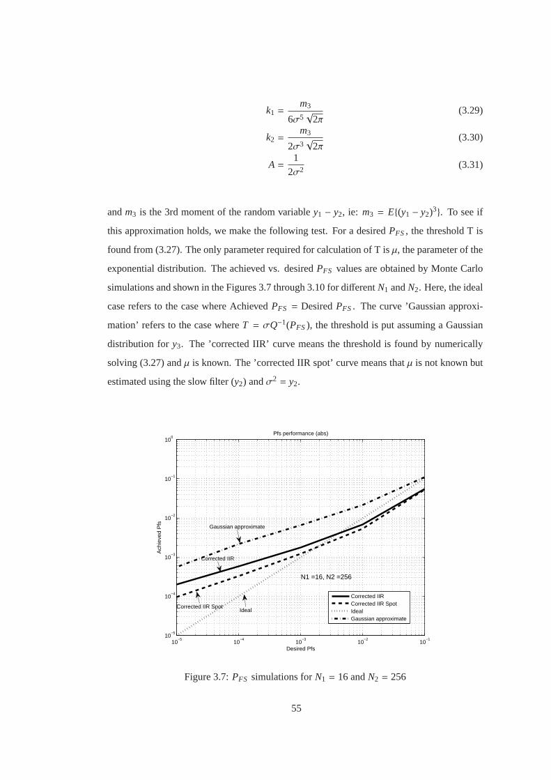
k1 =m3

6σ5√

2π(3.29)

k2 =m3

2σ3√

2π(3.30)

A =1

2σ2(3.31)

andm3 is the 3rd moment of the random variabley1 − y2, ie: m3 = E{(y1 − y2)3}. To see if

this approximation holds, we make the following test. For a desiredPFS , the threshold T is

found from (3.27). The only parameter required for calculation of T isµ, the parameter of the

exponential distribution. The achieved vs. desiredPFS values are obtained by Monte Carlo

simulations and shown in the Figures 3.7 through 3.10 for differentN1 andN2. Here, the ideal

case refers to the case where AchievedPFS = DesiredPFS . The curve ’Gaussian approxi-

mation’ refers to the case whereT = σQ−1(PFS ), the threshold is put assuming a Gaussian

distribution fory3. The ’corrected IIR’ curve means the threshold is found by numerically

solving (3.27) andµ is known. The ’corrected IIR spot’ curve means thatµ is not known but

estimated using the slow filter (y2) andσ2 = y2.

10−5

10−4

10−3

10−2

10−1

10−5

10−4

10−3

10−2

10−1

100

Pfs performance (abs)

Desired Pfs

Ach

ieve

d P

fs

N1 =16, N2 =256

Corrected IIRCorrected IIR SpotIdealGaussian approximate

Gaussian approximate

Corrected IIR

Corrected IIR SpotIdeal

Figure 3.7:PFS simulations forN1 = 16 andN2 = 256

55

10−5

10−4

10−3

10−2

10−1

10−5

10−4

10−3

10−2

10−1

100

Pfs performance (abs)

Desired Pfs

Ach

ieve

d P

fs

N1 =32, N2 =256

Corrected IIRCorrected IIR SpotIdealGaussian Approximate

Gaussian approximate

Corrected IIR

Corrected IIR Spot

Ideal

Figure 3.8:PFS simulations forN1 = 32 andN2 = 256

10−5

10−4

10−3

10−2

10−1

10−6

10−5

10−4

10−3

10−2

10−1

100

Pfs performance (abs)

Desired Pfs

Ach

ieve

d P

fs

N1 =64, N2 =256

Corrected IIRCorrected IIR SpotIdealGaussian Approximate

Gaussian approximate

Corrected IIR

Ideal

Corrected IIR Spot

Figure 3.9:PFS simulations forN1 = 64 andN2 = 256

56

10−5

10−4

10−3

10−2

10−1

10−6

10−5

10−4

10−3

10−2

10−1

100

Pfs performance (abs)

Desired Pfs

Ach

ieve

d P

fs

N1 =128, N2 =256

Corrected IIRCorrected IIR SpotIdealGaussian Approximate

Gaussian approximate

Corrected IIR

Corrected IIR Spot

Ideal

Figure 3.10:PFS simulations forN1 = 128 andN2 = 256

Figures 3.7 through 3.10 show us that the additional terms to the pdf shown in (3.11) have

improved our approximation of the original pdf. This also means that the threshold T for

(3.10) can be set using (3.27) for a wide range ofPFS values and for differentN1 and N2.

What is interesting is that, for some situations the ’Corrected IIR Spot’ curveis closer to the

ideal curve than the ’Corrected IIR’ curve. This is due to the fact that sincey2 is averaging a

large number of samples, its estimate of the noise variance can be better than thetheoretical

variance itself, for that particular time instant. Also, numerically solving (3.27), one can see

that there is a highly linear relationship betweenσ2 andT for a givenPFS . Since we use

y2 = σ2, this means a linear relationship can be used to determine the threshold from output

of y2 for a givenPFS . In other wordsT [n] ≃ cy2[n] wherec is found from Table 3.1.

Now, the SIIR CFAR algorithm can be summarized as shown in Figure 3.11. Here y1[n] is

the fast filter andy2[n] is the slow filter. (ie:N1 < N2). z[n] is the magnitude squared input

andT [n] is the threshold at timen.

57

Table 3.1: The linear multiplier forN2 = 256 andN1 for {16,32,64,128} to achieve a desiredPFS

PFS

N1 1.00E-001 1.00E-002 1.00E-003 1.00E-004 1.00E-00516 1.1289 1.0073 0.8652 0.6873 0.425332 0.7142 0.6351 0.5426 0.4270 0.262464 0.4053 0.3594 0.3057 0.2390 0.1470128 0.1725 0.1526 0.1294 0.1007 0.0622

1. Initializey1[0], y2[0],T [0]

2. For desiredN1 andN2 computeγ1 andγ2 from (3.3)

3. For desiredPFA computeα1 andα2 from (3.7)

4. For desiredPFS computec from Table 3.1

5. Updatey1 andy2 as

y1[n] = γ1y1[n − 1] + (1− γ1)z[n]

y2[n] = γ2y2[n − 1] + (1− γ2)z[n]

6. if |y1[n − 1] − y2[n − 1]| > cy2[n − 1]

• then T [n] = α2y2[n]

• else T [n] = α1y1[n]

7. Detection decision is based on:z[n]H1

≷H0

T [n − 1]

Figure 3.11: The SIIR CFAR algorithm explained

58

A block diagram implementation of the switching algorithm can be seen in Figure 3.12. Both

of the filters are running and the output is switched between two of them. This switching

decision is based on|y1 − y2| as explained before. This concludes the construction of the

Switching IIR CFAR algorithm. Figure 3.13 shows the behavior of SIIR CFARunder a clut-

ter edge. Simulation results are presented in the next chapter.

z[n]

y2[n] y2[n− 1]

α2y2[n− 1]

Comparator

1− γ2

γ2

α2z−1

y1[n] y1[n− 1]

α1y1[n− 1]

1− γ1

γ1

α1z−1

T [n]

Select (S)

S=1

S=0

Figure 3.12: Block diagram implementation of the switching algorithm

0 0.5 1 1.5 2 2.5 3−25

−20

−15

−10

−5

0

5

10

15

20

Time (sec)

Pow

er (

dB)

IIR CFAR Threshold Behaviour

N1=32 N2=256 FFT MagnitudeIIR Filter(Fast)IIR Filter (Slow)IIR SwitchIdeal Threshold

Use slow filter here

Use fast filter here

Figure 3.13: SIIR CFAR at work

59

CHAPTER 4

SIMULATION RESULTS

All simulations are performed in MATLAB 7.9.0 (R2009b). The simulation resultsof the

original SIIR CFAR algorithm are mentioned in Sections 4.2 through 4.4.

4.1 False alarm probability under homogeneous conditions

The false alarm probability under homogeneous environment of the SIIR CFAR algorithm is

the same as that of Slow IIR CFAR and Fast IIR CFAR because both of the filters y1 and

y2 are tuned to operate in the same false alarm probability. Figure 4.1 verifies thisline of

thought. The false alarm probability does not change because of the switching operation.

This is intuitively correct since with some probabilityp, the first filter is selected and with

some probability 1− p the second filter is selected. The false alarm probabilities of both of

these filters are the same, therefore the combined switching detector also hasthe same false

alarm probability.

60

10−6

10−5

10−4

10−3

10−2

10−1

100

10−6

10−5

10−4

10−3

10−2

10−1

100

Desired Pfa

Ach

ieve

d P

fa

Pfa for SIIR CFAR under homogeneous environment

SimNum = 1E8

Figure 4.1: Pfa for SIIR CFAR under homogeneous environment

4.2 False alarm probability under clutter edge

4.2.1 Simulation Setup

The downfall of using a single IIR filter with large N, is the excessive falsealarms under a

clutter edge. The SIIR CFAR algorithm should solve that problem. For algorithms that use

windows which span both the leading and lagging samples, the deviation in falsealarm proba-

bility can both be a decrease or an increase. The false alarm probability can increase, because

the test cell can be in the high clutter region but the threshold may be estimated using the low

clutter cells therefore causing a too small threshold estimate a false alarm. The false alarm

probability can also decrease because the test cell may be in the low clutter region and the

threshold may be estimated using the high clutter cells, therefore causing a too high threshold

and too small false alarm probability.

Since we are using causal IIR filters with no delay, we are not considering the ’leading win-

dow’, we only consider the lagging window or ’only the past’. Therefore, the false alarm

61

simulations done in [18] or [19] are not valid in our case. A new definition ofPFA in clutter

edge is required and is made in the following sense. First of all, remember thatwe are using

two filters, with approximate lengthsN1 and N2 and N2 > N1. During a clutter transition,

it is expected that afterN2 cells has passed, both of the filters will be settled and the false

alarm probability returns back to its design value. To assess this, the false alarm probability

of numerous test cells will be simulated. Figure 4.2 will be helpful. This shows the simula-

tion setup for particular values of the parameters. The false alarm probabilities of the cells

for different time instances will be found by simulation. This will show the change in the

obtained false alarm probability versus time. Obviously, just after the clutter edge has passed,

the false alarm probability will increase due to the fact that the threshold is stillin the process

of adapting and it is too low. After some time, it is expected that the threshold will settle down

and false alarm probability will approach to its steady state level.

0 0.5 1 1.5 2 2.5 3 3.5 4−20

−15

−10

−5

0

5

10

15

20

25

30

Time (sec)

Pow

er (

dB)

IIR CFAR Threshold Behaviour

N1=32 N2=256FFT MagnitudeIIR Filter(Fast)IIR Filter (Slow)IIR SwitchIdeal Threshold

Clutter transition at 1 sec

Figure 4.2: Pfa under clutter edge simulation setup

The clutter cells are modeled as exponential random variables with the following pdf.

62

fz(z) =1λ

exp(−zλ

)

where

λ =

β2, for lower clutter region

β2(1+C), for higher clutter region

Herez[n] is the magnitude squared DFT outputs of a single frequency bin,β2 is the total noise

power andC is the clutter-to-thermal noise ratio (CNR). For all of the simulations,β2 = 1

is used. For clutter edge simulations, it is assumed that there are no targets. The simulation

results will be in the form of achievedPFA versus time, for a fixed desiredPFA. There are

four variables that affect the outcome of the simulation results. These are

• DesiredPFA

• PFS

• N1 andN2

• CNR

Each item is varied while keeping the others fixed and simulation results are obtained.

4.2.2 Simulation Results

Using the simulation setup explained in 4.2.1, the following results are obtained.

63

4.2.2.1 Effect of varying PFA

0 0.5 1 1.5 2 2.5 3 3.5 410

−4

10−3

10−2

10−1

100

SIIR CFAR Pfa in Clutter Edge

Time (sec)

Pro

babi

lity

of F

alse

Ala

rm, P

fa

N1 =32, N2 =256

Pfa = 1e−2

Pfs = 1e−4

CNR =10dB

SwitchFast IIRSlow IIRIdeal

Figure 4.3:PFA simulations under clutter edge forN1 = 32, N2 = 256,PFA = 10−2,CNR=

10dB,PFS = 10−4

0 0.5 1 1.5 2 2.5 3 3.5 4

10−4

10−3

10−2

10−1

100

SIIR CFAR Pfa in Clutter Edge

Time (sec)

Pro

babi

lity

of F

alse

Ala

rm, P

fa

N1 =32, N2 =256

Pfa = 1e−3

Pfs = 1e−4

CNR =10dB

SwitchFast IIRSlow IIRIdeal

Figure 4.4:PFA simulations under clutter edge forN1 = 32, N2 = 256,PFA = 10−3,CNR=

10dB,PFS = 10−4

64

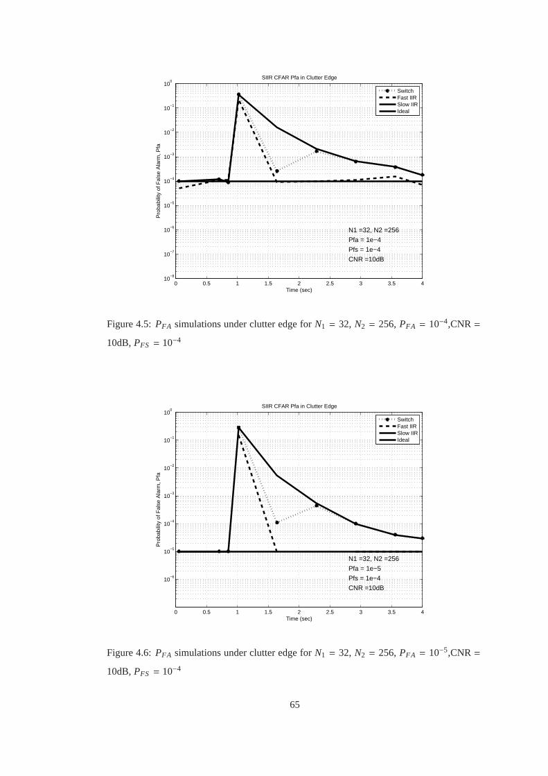
0 0.5 1 1.5 2 2.5 3 3.5 410

−8

10−7

10−6

10−5

10−4

10−3

10−2

10−1

100

SIIR CFAR Pfa in Clutter Edge

Time (sec)

Pro

babi

lity

of F

alse

Ala

rm, P

fa

N1 =32, N2 =256

Pfa = 1e−4

Pfs = 1e−4

CNR =10dB

SwitchFast IIRSlow IIRIdeal

Figure 4.5:PFA simulations under clutter edge forN1 = 32, N2 = 256,PFA = 10−4,CNR=

10dB,PFS = 10−4

0 0.5 1 1.5 2 2.5 3 3.5 4

10−6

10−5

10−4

10−3

10−2

10−1

100

SIIR CFAR Pfa in Clutter Edge

Time (sec)

Pro

babi

lity

of F

alse

Ala

rm, P

fa

N1 =32, N2 =256

Pfa = 1e−5

Pfs = 1e−4

CNR =10dB

SwitchFast IIRSlow IIRIdeal

Figure 4.6:PFA simulations under clutter edge forN1 = 32, N2 = 256,PFA = 10−5,CNR=

10dB,PFS = 10−4

65

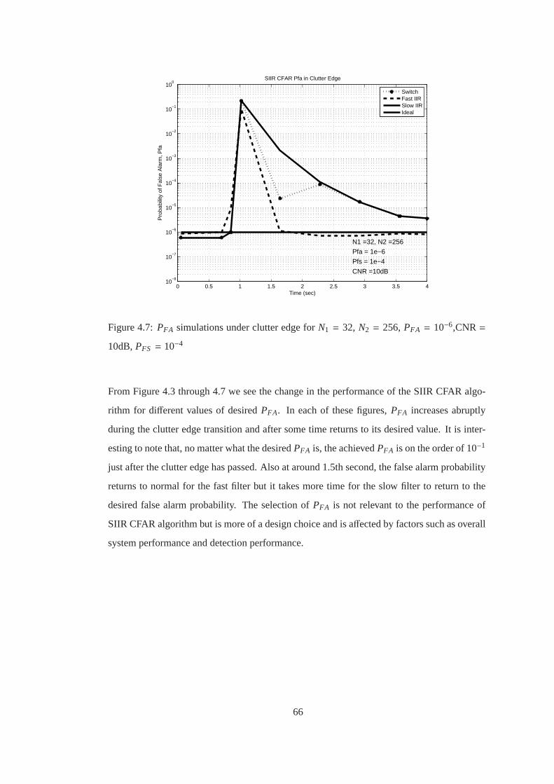
0 0.5 1 1.5 2 2.5 3 3.5 410

−8

10−7

10−6

10−5

10−4

10−3

10−2

10−1

100

SIIR CFAR Pfa in Clutter Edge

Time (sec)

Pro

babi

lity

of F

alse

Ala

rm, P

fa

N1 =32, N2 =256

Pfa = 1e−6

Pfs = 1e−4

CNR =10dB

SwitchFast IIRSlow IIRIdeal

Figure 4.7:PFA simulations under clutter edge forN1 = 32, N2 = 256,PFA = 10−6,CNR=

10dB,PFS = 10−4

From Figure 4.3 through 4.7 we see the change in the performance of the SIIR CFAR algo-

rithm for different values of desiredPFA. In each of these figures,PFA increases abruptly

during the clutter edge transition and after some time returns to its desired value.It is inter-

esting to note that, no matter what the desiredPFA is, the achievedPFA is on the order of 10−1

just after the clutter edge has passed. Also at around 1.5th second, the false alarm probability

returns to normal for the fast filter but it takes more time for the slow filter to return to the

desired false alarm probability. The selection ofPFA is not relevant to the performance of

SIIR CFAR algorithm but is more of a design choice and is affected by factors such as overall

system performance and detection performance.

66

4.2.2.2 Effect of varying PFS

0 0.5 1 1.5 2 2.5 3 3.5 410

−8

10−7

10−6

10−5

10−4

10−3

10−2

10−1

100

SIIR CFAR Pfa in Clutter Edge

Time (sec)

Pro

babi

lity

of F

alse

Ala

rm, P

fa

N1 =32, N2 =256

Pfa = 1e−4

Pfs = 1e−3

CNR =10dB

SwitchFast IIRSlow IIRIdeal

Figure 4.8:PFA simulations under clutter edge forN1 = 32, N2 = 256,PFA = 10−4,CNR=

10dB,PFS = 10−3

0 0.5 1 1.5 2 2.5 3 3.5 410

−8

10−7

10−6

10−5

10−4

10−3

10−2

10−1

100

SIIR CFAR Pfa in Clutter Edge

Time (sec)

Pro

babi

lity

of F

alse

Ala

rm, P

fa

N1 =32, N2 =256

Pfa = 1e−4

Pfs = 1e−5

CNR =10dB

SwitchFast IIRSlow IIRIdeal

Figure 4.9:PFA simulations under clutter edge forN1 = 32, N2 = 256,PFA = 10−4,CNR=

10dB,PFS = 10−5

67

It can be seen from Figures 4.8, 4.5 and 4.9, that changingPFS does change the performance

of the SIIR CFAR slightly during a clutter transition. All of the figures above show that until

up to 1.5th second, the fast filter is selected and after around 3rd second, the slow filter is se-

lected. What happens in betweent = 1.5 andt = 3 is decided by the setPFS . As expected, an

increase inPFS means, more switching decisions are performed and the fast filter is selected

more frequently. Therefore, the false alarm probability will be closer to that of the fast filter

asPFS is increased. This is validated by the performed simulations.

4.2.2.3 Effect of varying N1

0 0.5 1 1.5 2 2.5 3 3.5 410

−8

10−7

10−6

10−5

10−4

10−3

10−2

10−1

100

SIIR CFAR Pfa in Clutter Edge

Time (sec)

Pro

babi

lity

of F

alse

Ala

rm, P

fa

N1 =64, N2 =256

Pfa = 1e−4

Pfs = 1e−4

CNR =10dB

SwitchFast IIRSlow IIRIdeal

Figure 4.10:PFA simulations under clutter edge forN1 = 64, N2 = 256,PFA = 10−4,CNR=

10dB,PFS = 10−4

68

0 0.5 1 1.5 2 2.5 3 3.5 410

−8

10−7

10−6

10−5

10−4

10−3

10−2

10−1

100

SIIR CFAR Pfa in Clutter Edge

Time (sec)

Pro

babi

lity

of F

alse

Ala

rm, P

fa

N1 =128, N2 =256

Pfa = 1e−4

Pfs = 1e−4

CNR =10dB

SwitchFast IIRSlow IIRIdeal

Figure 4.11:PFA simulations under clutter edge forN1 = 128,N2 = 256,PFA = 10−4,CNR

= 10dB,PFS = 10−4

It can be seen from Figures 4.5, 4.10 and 4.11 that changingN1 has the effect of ’delaying’

the transition point from the fast filter to the slow filter. This is also expected because asN1

increases, the update rate of the fast filter decreases. Initially, in the beginning of the clutter

edge the difference|y1 − y2| is large, therefore the fast filter is selected. For smallN1, this

difference decreases quickly because the update rate of the fast filter is large. For largeN1,

however, it takes more time for this difference to become small and therefore the switching

point from the fast filter to the slow filter is delayed. It can be seen that in Figure 4.5, this

switching point is at 1.5th second, in Figure 4.10 the switching point is at 2.25th second and

in Figure 4.11 the switching point is at 3.5th second. These findings support our initial pre-

dictions.

69

4.2.2.4 Effect of varying CNR

0 0.5 1 1.5 2 2.5 3 3.5 410

−8

10−7

10−6

10−5

10−4

10−3

10−2

10−1

100

SIIR CFAR Pfa in Clutter Edge

Time (sec)

Pro

babi

lity

of F

alse

Ala

rm, P

fa

N1 =32, N2 =256

Pfa = 1e−4

Pfs = 1e−4

CNR =5dB

SwitchFast IIRSlow IIRIdeal

Figure 4.12:PFA simulations under clutter edge forN1 = 32, N2 = 256,PFA = 10−4,CNR=

5dB, PFS = 10−4

0 0.5 1 1.5 2 2.5 3 3.5 410

−8

10−7

10−6

10−5

10−4

10−3

10−2

10−1

100

SIIR CFAR Pfa in Clutter Edge

Time (sec)

Pro

babi

lity

of F

alse

Ala

rm, P

fa

N1 =32, N2 =256

Pfa = 1e−4

Pfs = 1e−4

CNR =7dB

SwitchFast IIRSlow IIRIdeal

Figure 4.13:PFA simulations under clutter edge forN1 = 32, N2 = 256,PFA = 10−4,CNR=

7dB, PFS = 10−4

70

Figures 4.12, 4.13 and 4.5 show the simulation results when CNR values of 10dB, 7dB and

5dB are used respectively. As expected, the false alarm increase in theclutter edge is directly

proportional with CNR value. (ie: as CNR increases, so doesPFA under clutter edge). The

switching from fast filter to the slow filter happens at the same point for different CNR values.

4.3 Probability of detection under homogeneous conditions

4.3.1 Simulation Setup

The detection probabilityPD under homogeneous conditions is simulated as follows. The pdf

of z[n] in this case is:

fz(z) =1λ

exp(−zλ

)

where

λ =

β2, underH0

β2(1+ S ), underH1

whereS is the average signal to noise ratio (SNR) of the target as in [42]. In otherwords,

Swerling 1 model [43] is assumed for the radar returns.β2 = 1 is used for all the simulations.

The clutter is assumed to be uniform and there are no interfering targets. The probability of

detection under homogeneous conditions is expected to be very close to the ideal case. This

is shown in the following figures.

71

4.3.2 Simulation Results

4.3.2.1 Effect of varying PFA

0 5 10 15 20 25 300

0.1

0.2

0.3

0.4

0.5

0.6

0.7

0.8

0.9

1SIIR CFAR Pd in Homogeneous Environment

SNR (dB)

Pro

babi

lity

of D

etec

tion,

Pd

N1 =32, N2 =256

Pfa = 1e−4

Pfs = 1e−4

Fast IIRSlow IIRSwitching IIRIdeal

Figure 4.14: PD simulations forN1 = 32, N2 = 256, PFA = 10−4, PFS = 10−4 under

homogeneous conditions

0 5 10 15 20 25 300

0.1

0.2

0.3

0.4

0.5

0.6

0.7

0.8

0.9

1SIIR CFAR Pd in Homogeneous Environment

SNR (dB)

Pro

babi

lity

of D

etec

tion,

Pd

N1 =32, N2 =256

Pfa = 1e−5

Pfs = 1e−4

Fast IIRSlow IIRSwitching IIRIdeal

Figure 4.15: PD simulations forN1 = 32, N2 = 256, PFA = 10−5, PFS = 10−4 under

homogeneous conditions

72

0 5 10 15 20 25 300

0.1

0.2

0.3

0.4

0.5

0.6

0.7

0.8

0.9

1SIIR CFAR Pd in Homogeneous Environment

SNR (dB)

Pro

babi

lity

of D

etec

tion,

Pd

N1 =32, N2 =256

Pfa = 1e−6

Pfs = 1e−4

Fast IIRSlow IIRSwitching IIRIdeal

Figure 4.16: PD simulations forN1 = 32, N2 = 256, PFA = 10−6, PFS = 10−4 under

homogeneous conditions

4.3.2.2 Effect of varying N1

0 2 4 6 8 10 12 14 16 18 200

0.1

0.2

0.3

0.4

0.5

0.6

0.7

0.8

0.9

1SIIR CFAR Pd in Homogeneous Environment

SNR (dB)

Pro

babi

lity

of D

etec

tion,

Pd

N1 =64, N2 =256

Pfa = 1e−4

Pfs = 1e−4

Fast IIRSlow IIRSwitching IIRIdeal

Figure 4.17: PD simulations forN1 = 64, N2 = 256, PFA = 10−4, PFS = 10−4 under

homogeneous conditions

73

0 2 4 6 8 10 12 14 16 18 200

0.1

0.2

0.3

0.4

0.5

0.6

0.7

0.8

0.9

1SIIR CFAR Pd in Homogeneous Environment

SNR (dB)

Pro

babi

lity

of D

etec

tion,

Pd

N1 =128, N2 =256

Pfa = 1e−4

Pfs = 1e−4

Fast IIRSlow IIRSwitching IIRIdeal

Figure 4.18: PD simulations forN1 = 128, N2 = 256, PFA = 10−4, PFS = 10−4 under

homogeneous conditions

4.3.2.3 Effect of varying PFS

0 2 4 6 8 10 12 14 16 18 200

0.1

0.2

0.3

0.4

0.5

0.6

0.7

0.8

0.9

1SIIR CFAR Pd in Homogeneous Environment

SNR (dB)

Pro

babi

lity

of D

etec

tion,

Pd

N1 =32, N2 =256

Pfa = 1e−4

Pfs = 1e−1

Fast IIRSlow IIRSwitching IIRIdeal

Figure 4.19: PD simulations forN1 = 32, N2 = 256, PFA = 10−4, PFS = 10−1 under

homogeneous conditions

74

0 2 4 6 8 10 12 14 16 18 200

0.1

0.2

0.3

0.4

0.5

0.6

0.7

0.8

0.9

1SIIR CFAR Pd in Homogeneous Environment

SNR (dB)

Pro

babi

lity

of D

etec

tion,

Pd

N1 =32, N2 =256

Pfa = 1e−4

Pfs = 1e−2

Fast IIRSlow IIRSwitching IIRIdeal

Figure 4.20: PD simulations forN1 = 32, N2 = 256, PFA = 10−4, PFS = 10−2 under

homogeneous conditions

As it is seen from Figures 4.14 through 4.18, the performance of SIIR CFAR is very close to

the ideal detector under homogeneous conditions. ChangingN1 does not affect this perfor-

mance greatly. The effect of changingPFS on detection performance is very minimal. Ob-

viously asPFS decreases, the slower filter will tend to get selected more often and therefore

the detection performance will increase. IncreasingPFS will lead to a decrease in detection

performance however this effect is very subtle and can be omitted. As explained before, the

selection ofPFA is not relevant to the performance of SIIR CFAR algorithm but is more of

a design choice and is affected by factors such as overall system performance and detection

performance.

75

4.4 Probability of detection under interfering targets

In the presence of interfering targets,PD is not expected to change because the threshold is

not updated when a target present decision is made.

The simulation setup is seen in Figure 4.21.

0 0.5 1 1.5 2 2.5 3 3.5 4−25

−20

−15

−10

−5

0

5

10

15

20

25

Time (sec)

Pow

er (

dB)

IIR CFAR Threshold Behaviour

N1=32 N2=256

INR = SNR =20dB

FFT MagnitudeIdeal Threshold

Interfering Target

0.5 secMain Target

Figure 4.21: Simulation setup for multiple targets

76

Here one interfering target is shown with a separation of 0.5 seconds.

0 5 10 15 20 25 300

0.1

0.2

0.3

0.4

0.5

0.6

0.7

0.8

0.9

1S−CMAP CFAR Pd Under Multiple Targets

SNR (dB)

Pro

babi

lity

of D

etec

tion,

Pd

N1 =32, N2 =256

Pfa = 1e−4

Pfs = 1e−4

INR = SNR

Target seperation =0.5 sec

Fast IIRSlow IIRSwitching IIRIdeal

Figure 4.22:PD simulations forN1 = 32, N2 = 256, PFA = 10−4, PFS = 10−4 under one

interfering target 0.5 second away

Since the threshold is not updated when there is a detection, there is no change inPD as seen

from Figure 4.22.

4.5 Comparison to other CFAR Algorithms

77

0 100 200 300 400 500 60010

−5

10−4

10−3

10−2

10−1

100

Range Bin

Fal

se A

larm

Pro

babi

lity

PFA under Clutter Edge for Different CFAR Algorithms

SIIR(128)Fast(32)Slow(128)SIIR(64)Fast(32)Slow(64)OS(24/32)OS(16/32)CA(32)

Slow (128)

Slow (64)

SIIR (64)SIIR (128)

Fast (32)

OS(16/32)

OS(24/32)

CA(32)

Clutter transition at 300th range binCNR = 10dB

Figure

4.23:PF

Asim

ulationsunder

clutteredge

forS

IIRC

FAR

vs.other

known

CFA

R

algorithms

78

CHAPTER 5

CONCLUSION

In this thesis, a new algorithm based on IIR filtering and a switching operationfor CFAR

detection of radar targets is presented, developed and analyzed. The relevant literature is re-

viewed in Chapter 2. The basics of CFAR detection using IIR filters is presented in Chapter

3. Most CFAR methods use some number of cells (or windows) to set a threshold and then

compare the cell under test against this threshold. This means storing at least the window size

number of cells and deciding accordingly. Memory requirement and computational demand

therefore increases. More advanced CFAR methods (such as ordered statistics or trimmed

mean detectors) use ordering of the samples in the window which means even more compu-

tation. The simplicity of using an IIR filter to estimate the noise background comes from the

fact that only a single value is kept in the memory and this value is updated. Theadvantages

and disadvantages of using IIR filters for detection are summarized in Chapter 3.

In Chapter 4, a new algorithm is proposed which uses two IIR filters with different time con-

stants to address some problems mentioned before. The main reasoning is as follows, two

IIR filters with different time constants (preferably one will have a time constant significantly

larger than the other one) react differently in a clutter edge environment. It is shown that the

slow filter has better detection performance than the fast filter under homogeneous conditions.

Also it is shown that the fast filter has better clutter edge performance (the excessive increase

of PFA under clutter edge is less) than slow filter. Therefore, it is advised to use the slow filter

for the homogeneous environment and the fast filter for the non homogeneous environment.

Then comes the problem of deciding whether the environment is homogeneous or not. This

79

can be done in terms of comparing the two filter outputs. The absolute value of the difference

between the two filter outputs can be used as a measure of homogeneity. In a homogeneous

environment, this difference is expected to be small whereas in a non homogeneous envi-

ronment this difference is expected to be large (due to the differences in the time constants).

What we aim to do is, use the slow filter when the difference is small and switch to the fast

filter when the difference is large. Then, a measure of ’switching’ can be developed as follows:

PFS = {|y1 − y2| > T ; Homogeneous Environment}

wherePFS is the probability of false switching,T is a predetermined switching threshold and

y1, y2 are the filter outputs. This probability is denoted as false switching probability because

when the environment is homogeneous, no switching operations are expected. Obviously,

whenPFS is increased, more switching decisions will commence. To findT , the analytical

pdfs ofy1 andy2 are required but to the best of my knowledge, analytical forms are not avail-

able.

An approximate pdf fory1 − y2 is developed in Chapter 4 and it is seen that a linear relation-

ship in the following form performs reasonably well for a large range of designPFS values.

PFS = {|y1 − y2| > cy2; Homogeneous Environment}

wherec can be determined both analytically and through approximations. Using this defini-

tion of PFS and calculatedc values, the Switching IIR CFAR (SIIR CFAR) algorithm design

is complete.

Chapter 5 contains the simulation results. Three main benchmarks were considered. These

are, detection under homogeneous conditions, detection under multiple targets and false alarm

probability under clutter edge. The detection probability under homogeneous conditions is

very close to the ideal case. The detection probability under multiple targets has no perfor-

mance degradation. The excessive false alarms under clutter edge is close to that of the Fast

80

IIR CFAR

As a summary, a new algorithm for CFAR detection of radar targets is developed in this thesis.

This algorithm uses two IIR filters and a switching operation to select which filter to use. The

main advantage of this algorithm is its computational simplicity, multiple target performance

and detection performance. There are algorithms that may perform better inthe presence of

clutter edges (because of the windowing structure), however efforts are made to increase the

clutter edge performance of the SIIR CFAR algorithm. In the future, theoretical approaches

to calculating false alarm probability could be investigated. It might also be worthwhile to

look into ”double exponential smoothers” (where two past samples are used instead of one)

[44] because they might perform better in clutter edges.

81

REFERENCES

[1] T Bayes. An essay towards solving a problem in the doctrine of chances. 1763.M.D.computing : computers in medical practice, 8(3):157–71.

[2] J. Neyman and E. S. Pearson. On the Problem of the Most Efficient Tests of Statisti-cal Hypotheses.Philosophical Transactions of the Royal Society of London. Series A,Containing Papers of a Mathematical or Physical Character, 231.

[3] Steven M. Kay. Fundamentals of Statistical Signal Processing, Volume 2: DetectionTheory. Prentice Hall, 1998.

[4] Mark A. Richards.Fundamentals of Radar Signal Processing. McGraw-Hill, 2005.

[5] Harry L. Van Trees. Detection, Estimation, and Modulation Theory, Part I. Wiley-Interscience, 2001.

[6] Nadav Levanon.Radar Principles. Wiley-Interscience, 1988.

[7] M. Weiss. Analysis of some modified cell-averaging CFAR processorsin multiple-targetsituations. IEEE Transactions on Aerospace and Electronic Systems, AES-18(1):102–114, January 1982.

[8] James Ritcey. Performance Analysis of the Censored Mean-Level Detector. IEEETransactions on Aerospace and Electronic Systems, AES-22(4):443–454, July 1986.

[9] John Rickard and George Dillard. Adaptive Detection Algorithms for Multiple-TargetSituations.IEEE Transactions on Aerospace and Electronic Systems, AES-13(4):338–343, July 1977.

[10] J Presley Jr. Automated detection in multiple-target environments using thecensoredmean-level detector.Acoustics, Speech, and Signal Processing, IEEE, pages 1–4, 2003.

[11] PP Gandhi and SA Kassam. Analysis of CFAR processors in nonhomogeneous back-ground.IEEE Transactions on Aerospace and Electronic Systems, 14(4), 1988.

[12] Fred E. Nathanson, J. Patrick Reilly, Cohen, and Marvin N.Radar Design Principles:Signal Processing and the Environment, Second Edition. SciTech Publishing, 1999.

[13] S.L. Wilson. Two CFAR algorithms for interfering targets and nonhomogeneous clutter.IEEE Transactions on Aerospace Electronic Systems, 29:57–72, 1993.

[14] Hermann Rohling. Radar CFAR thresholding in clutter and multiple target situations.IEEE Transactions on Aerospace and Electronic Systems, (4), 1983.

[15] S Blake. OS-CFAR theory for multiple targets and nonuniform clutter.IEEE Transac-tions on Aerospace Electronic Systems, 24(6):785–790, 1988.

82

[16] M. Shor and N. Levanon. Performances of order statistics CFAR.IEEE Transactionson Aerospace and Electronic Systems, 27(2):214–224, 1991.

[17] ME Smith and PK Varshney. VI-CFAR- A novel CFAR algorithm basedon data vari-ability. IEEE National Radar Conference, 1997.

[18] M.E. Smith and P.K. Varshney. Intelligent CFAR processor based ondata variability.IEEE Transactions on Aerospace and Electronic Systems, 36(3):837–847, July 2000.

[19] TTV Cao. Constant false-alarm rate algorithm based on test cell information.Engineer-ing and Technology, 2(3):200– 213, 2008.

[20] L.M. Novak. Radar target detection and map-matching algorithm studies. IEEE Trans-actions on Aerospace and Electronic Systems, AES-16(5):620–625, September 1980.

[21] V. Hansen and Harold Ward. Detection Performance of the Cell Averaging LOG/CFARReceiver.IEEE Transactions on Aerospace and Electronic Systems, AES-8(5):648–652,September 1972.

[22] HM Finn. A CFAR design for a window spanning two clutter fields.IEEE Transactionson Aerospace and Electronic Systems, (2):155–169, 1986.

[23] Ramon Nitzberg. Clutter Map CFAR Analysis.IEEE Transactions on Aerospace andElectronic Systems, AES-22(4):419–421, July 1986.

[24] E. Conte and M. Lops. Clutter-map CFAR detection for range-spread targets in non-Gaussian clutter. Part I: System design.IEEE Transactions on Aerospace and ElectronicSystems, 33(2):432–443, April 1997.

[25] M Lops. Hybrid clutter-map/L-CFAR procedure for clutter rejection in nonhomoge-neous environment.IEE Proceedings-Radar, Sonar and Navigation, 1996.

[26] D. Schleher. Harbor surveillance radar detection performance.IEEE Journal of OceanicEngineering, 2(4):318–325, October 1977.

[27] P.P. Gandhi, E. Cardona, and L. Baker. CFAR signal detection in nonhomogeneousWeibull clutter and interference.Proceedings International Radar Conference, 0:583–588.

[28] R. Rifkin. Analysis of CFAR performance in Weibull clutter.IEEE Transactions onAerospace and Electronic Systems, 30(2):315–329, April 1994.

[29] A. Sarma and D.W. Tufts. Robust adaptive threshold for control of false alarms.IEEESignal Processing Letters, 8(9):261–263, 2001.

[30] Anas Tom and R. Viswanathan. Switched order statistics CFAR test for target detection.IEEE Radar Conference, 2008., 2(1):1–5, May 2008.

[31] Yu-Zhen Song, Xiang-wei Meng, and Fu-yong Qu. A new CFAR method based on testcell statistics.IET Conference Publications, 1(2):426–426, 2009.

[32] A.R. Elias-Fuste, M.G.G. de Mercado, and E. de los Reyes Davo. Analysis of somemodified ordered statistic cfar: Osgo and osso cfar.Aerospace and Electronic Systems,IEEE Transactions on, 26(1):197 –202, January 1990.

83

[33] S. Erfanian and V.T. Vakili. Analysis of some CFAR detectors in nonhomogenous en-vironments based on switching algorithm.2009 International Multimedia, Signal Pro-cessing and Communication Technologies, (1):1–4, March 2009.

[34] A Farrouki and M Barkat. Automatic censored mean level detector using a variability-based censoring with non-coherent integration.Signal Processing, 87(6):1462–1473,June 2007.

[35] PP Gandhi and SA Kassam. Optimality of the cell averaging CFAR detector. IEEETransactions on Information Theory, 40(4):1226–1228, 2002.

[36] N. Levanon. Numerically efficient calculations of clutter map CFAR performance.Aerospace and Electronic Systems, IEEE Transactions on, (6):813–814, 1987.

[37] J Lehtomaki. Analysis of energy based signal detection.Department of Electrical andInformation, 2005.

[38] J.J. Lehtomaki, M. Juntti, H. Saarnisaari, and S. Koivu. Thresholdsetting strategies fora quantized total power radiometer.IEEE Signal Processing Letters, 12(11):796–799,November 2005.

[39] M Lops and M Orsini. Scan-by-scan averaging CFAR.IEE Proceedings For Radar andSignal Processing, (6), 1989.

[40] Athanasios Papoulis and S.Unnikrishna Pillai.Probability, Random Variables andStochastic Processes. McGraw Hill Higher Education, 2002.

[41] Ronald L. Graham, Donald E. Knuth, and Oren Patashnik.Concrete Mathematics:Foundation for Computer Science. Addison Wesley, 1994.

[42] H. Goldman. Performance of the excision CFAR detector in the presence of interferers.In Radar and Signal Processing, IEE Proceedings F, volume 137, pages 163–171. IET,2002.

[43] P Swerling. Probability of detection for fluctuating targets.Information Theory, IRETransactions on, 2002.

[44] Joseph J. LaViola. Double exponential smoothing: an alternative to kalman filter-basedpredictive tracking. InProceedings of the workshop on Virtual environments 2003,EGVE ’03, pages 199–206, New York, NY, USA, 2003. ACM.

84