CFD ANALYSIS Of COMBINED 8-12 STAGES Of · PDF fileCFD ANALYSIS Of COMBINED 8-12 STAGES Of INTERMIDIATE PRESSURE STEAM TURBINE ... I. Introduction %+ ... The blade of the Utility IP

NCADOMS-2016 Special Issue 1 Page 21

CFD ANALYSIS Of COMBINED 8-12 STAGES Of

INTERMIDIATE PRESSURE STEAM TURBINE

1st Author name : SHIVAKUMAR VASMATE, 2

nd Author name : KAMALADEVI

ANANDE.

1 Department of Mechanical Engineering, India

2 Department of Civil Engineering, India

ABSTRACT

Steam Turbines play a vital role in power generation as a prime mover which converts kinetic energy

of steam into mechanical energy. Many of the utility steam turbines is the combination of three

cylinder construction i.e. High pressure cylinder in which pressure is maximum with minimum

specific volume and so blade height is minimum, Intermediate pressure cylinder in which pressure is

intermediate and so is the blade height and finally low pressure cylinder which has a minimum

pressure level and maximum specific volume and hence maximum blade height. Generally, IP Steam

turbine consists of 12 stages; combination of 1-7 stages and 8-12 stages which are divided by the use

of the extraction strip. A typical Intermediate Pressure cylinder module is chosen to carry out the

project work.

The flow in a Turbine blade passage is complex and involves understanding of energy

conversion in three dimensional geometries. The performance of the turbine depends on the efficient

conversion with minimum amount of flow losses. To improve the performance it is essential to

identify the losses generating mechanism and study their influence and effects on performance. The

objective of the project is to carry out the CFD analysis of a typical IP utility turbine module

considering the hub/shroud sealing between the stages which account for leakage losses.

To achieve the above objective we need to model separately the bladed region and attach the

hub/shroud seal region to it by General Grid Interface. The flow domain and mesh generation for

seal area needs to be accurate to get the correct interface with blades. IDEAS software is used for

geometric modeling, CFX-TURBOGRID software is used for meshing the blade region, ICEM-CFD

software is used for meshing the hub/shroud region of the seals and CFX is used for physics

definition and solving the problem. Initially the analysis is carried out for the 8th stage, subsequently

for the combined 8-12 stages. The results are compared with two dimensional (2D) analysis

calculations and found.

Keywords-Steam turbine, Hub/shroud, General Grid Interface (GGI), IDEAS software, CFX TURBO-GRID

software, ICEM-CFD software, CFX software


I. Introduction

BHEL is manufacturing a wide variety of turbines over the last 50 years to meet India’s growing need for power. Steam turbine plays a vital role in power generation as a prime mover, which

converts Kinetic Energy of steam to Mechanical Energy. Many of the utility steam turbines are of

three cylinder constructions i.e. High pressure cylinder in which pressure is maximum with

minimum specific volume and so blade height is minimum, Intermediate pressure cylinder in which

pressure is intermediate so the blade height is intermediate and Low pressure cylinder which has a

minimum pressure level & maximum specific volume and hence LP cylinder blade height is

maximum.

A typical Intermediate pressure Turbine of utility steam turbine is chosen to carry out the

CFD analysis. The analysis requires solving of fluid problem in bladed region. This can be done in

three approaches, Analytical, Experimental and Numerical. Analytical methods which assume a

continuum hypothesis are more suited for simple problems and are not suited for complex fluid flow

problems. Experimental methods are suited for complex fluid flow problems but the expenditure for

carrying out the analysis is high. The other limitation is that the determination of the fluid

characteristics in the interiors becomes complex and difficult. Hence, Numerical approach is more

feasible approach for analysis of a particular design because it overcomes the limitations of the two

methods and it gives a close approximate for complex form of fluid problems too. Numerical

approach involves discretization of the governing mathematical equations gives numerical solutions

for the flow problems.

The analysis is carried out by identifying the flow domain. The domain is modeled, discretized and

governing equations are solved using commercially available software. The results are post

processed and compared with 2 dimensional program results which were experimentally verified.

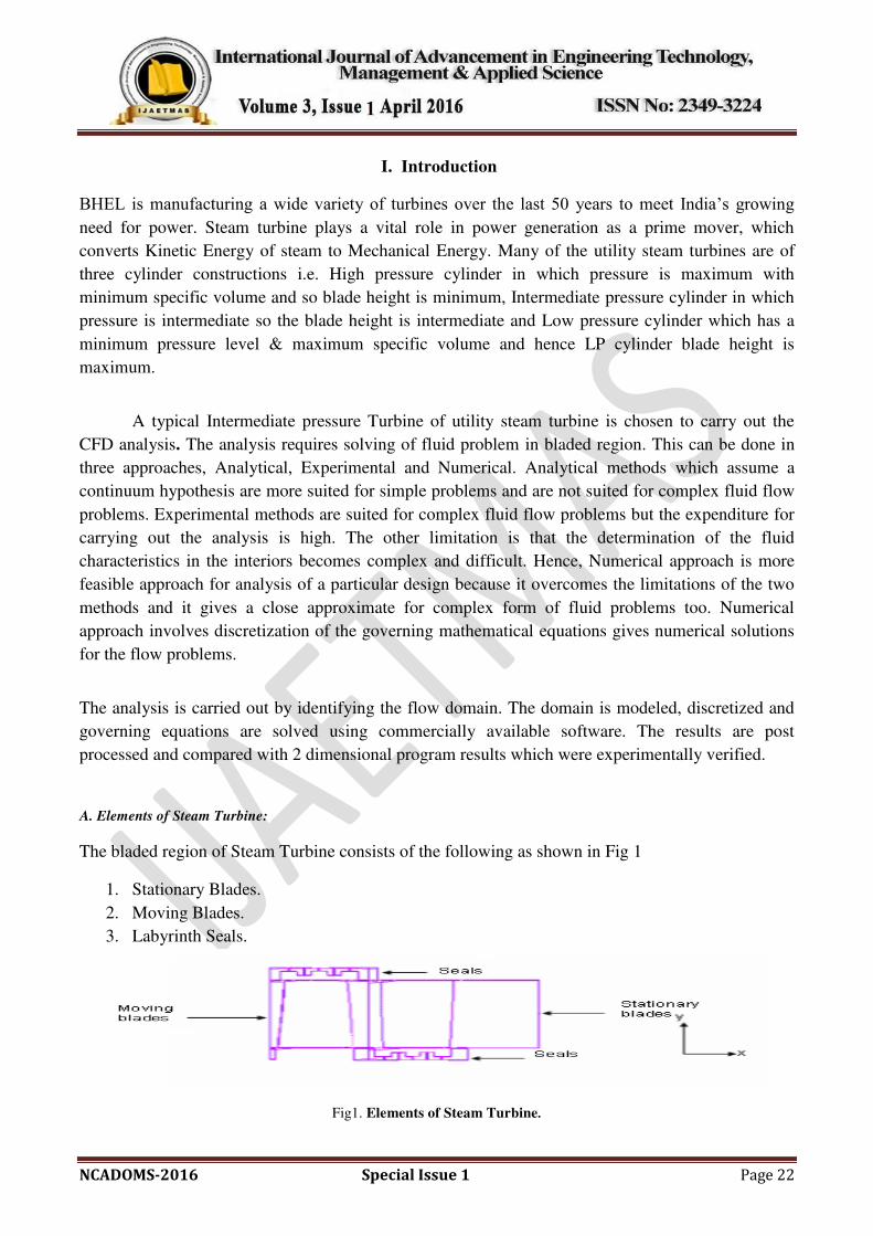
A. Elements of Steam Turbine:

The bladed region of Steam Turbine consists of the following as shown in Fig 1

1. Stationary Blades.

2. Moving Blades.

3. Labyrinth Seals.

Fig1. Elements of Steam Turbine.


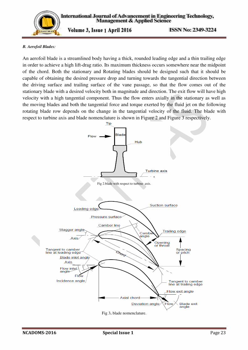
B. Aerofoil Blades:

An aerofoil blade is a streamlined body having a thick, rounded leading edge and a thin trailing edge

in order to achieve a high lift-drag ratio. Its maximum thickness occurs somewhere near the midpoint

of the chord. Both the stationary and Rotating blades should be designed such that it should be

capable of obtaining the desired pressure drop and turning towards the tangential direction between

the driving surface and trailing surface of the vane passage, so that the flow comes out of the

stationary blade with a desired velocity both in magnitude and direction. The exit flow will have high

velocity with a high tangential component. Thus the flow enters axially in the stationary as well as

the moving blades and both the tangential force and torque exerted by the fluid jet on the following

rotating blade row depends on the change in the tangential velocity of the fluid. The blade with

respect to turbine axis and blade nomenclature is shown in Figure 2 and Figure 3 respectively.

Fig 2.blade with respect to turbine axis.

Fig 3. blade nomenclature.


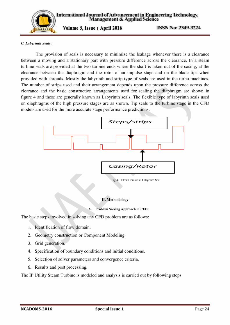
C. Labyrinth Seals:

The provision of seals is necessary to minimize the leakage whenever there is a clearance

between a moving and a stationary part with pressure difference across the clearance. In a steam

turbine seals are provided at the two turbine ends where the shaft is taken out of the casing, at the

clearance between the diaphragm and the rotor of an impulse stage and on the blade tips when

provided with shrouds. Mostly the labyrinth and strip type of seals are used in the turbo machines.

The number of strips used and their arrangement depends upon the pressure difference across the

clearance and the basic construction arrangements used for sealing the diaphragm are shown in

figure 4 and these are generally known as Labyrinth seals. The flexible type of labyrinth seals used

on diaphragms of the high pressure stages are as shown. Tip seals to the turbine stage in the CFD

models are used for the more accurate stage performance predictions.

Fig 4. : Flow Domain at Labyrinth Seal

II. Methodology

A. Problem Solving Approach in CFD:

The basic steps involved in solving any CFD problem are as follows:

1. Identification of flow domain.

2. Geometry construction or Component Modeling.

3. Grid generation.

4. Specification of boundary conditions and initial conditions.

5. Selection of solver parameters and convergence criteria.

6. Results and post processing.

The IP Utility Steam Turbine is modeled and analysis is carried out by following steps


1. Identification of Flow Domain:

Before constructing grid, it is required to understand the exact flow domain properly. The flow

domain in the case of Steam Turbine consists of blade path (both Stationary and Rotating blades

fixed to casing and rotor respectively), Labyrinth seals, and steam inlet & outlet. It is therefore

required that before going ahead with 3D modeling and grid generation, the common interfaces

should be clearly defined between each blade in each stage and seals. The software that is used for

generating the geometry and meshing is decided based on nature and complexity of the geometry.

For axi-symmetry bladed geometry, the data for hub, shroud and blade profiles are obtained from 2D

drawing and subsequently grids are generated using Turbo-Grid software. Though the stage consists

of Stationary and Rotating blades, but to get the flow developed to the upstream of the hub a small

passage is added and similarly to the downstream of the shroud the flow domain is extended up to

some distance, so that realistic boundary conditions can be given at the inlet and outlet surfaces. The

boundary wall is the region where no slip condition exists and the velocity gradually increases and

reaches to mainstream velocities. That means, velocity gradient exists there and that region close to

the boundary wall should have fine grids to capture the boundary wall effects.

2. Geometrical Modeling:

In order to analyze the flow and to evaluate the performance, basically three steps are required

as follows:

1. Modeling of components.

2. Grid generation.

3. Analysis.

4.

As the flow domain consists of blade and seal passages, the modeling is carried out as described

below:

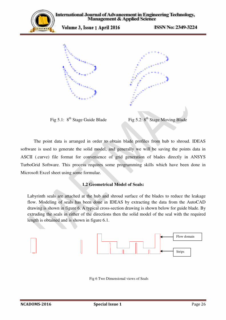
1.1. Geometrical Model of Blades:

The blade of the Utility IP Steam Turbine is of cylindrical type and blade extends between hub

and shroud surfaces. The geometry of blade is extracted from blade profile co-ordinates are shown in

figure 5.1 and figure 5.2, given in the form of suction side and pressure side points, which are located

along the radial positions of the blade.


Fig 5.1: 8th

Stage Guide Blade Fig 5.2: 8th

Stage Moving Blade

The point data is arranged in order to obtain blade profiles from hub to shroud. IDEAS

software is used to generate the solid model, and generally we will be saving the points data in

ASCII (.curve) file format for convenience of grid generation of blades directly in ANSYS

TurboGrid Software. This process requires some programming skills which have been done in

Microsoft Excel sheet using some formulae.

1.2 Geometrical Model of Seals:

Labyrinth seals are attached at the hub and shroud surface of the blades to reduce the leakage

flow. Modeling of seals has been done in IDEAS by extracting the data from the AutoCAD

drawing is shown in figure 6. A typical cross-section drawing is shown below for guide blade. By

extruding the seals in either of the directions then the solid model of the seal with the required

length is obtained and is shown in figure 6.1.

Fig 6 Two Dimensional views of Seals

Flow domain

Strips


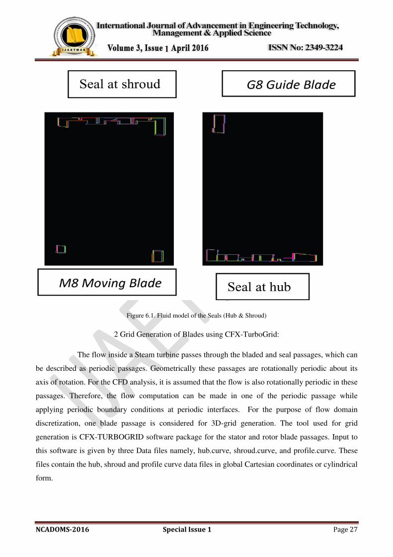
Figure 6.1. Fluid model of the Seals (Hub & Shroud)

2 Grid Generation of Blades using CFX-TurboGrid:

The flow inside a Steam turbine passes through the bladed and seal passages, which can

be described as periodic passages. Geometrically these passages are rotationally periodic about its

axis of rotation. For the CFD analysis, it is assumed that the flow is also rotationally periodic in these

passages. Therefore, the flow computation can be made in one of the periodic passage while

applying periodic boundary conditions at periodic interfaces. For the purpose of flow domain

discretization, one blade passage is considered for 3D-grid generation. The tool used for grid

generation is CFX-TURBOGRID software package for the stator and rotor blade passages. Input to

this software is given by three Data files namely, hub.curve, shroud.curve, and profile.curve. These

files contain the hub, shroud and profile curve data files in global Cartesian coordinates or cylindrical

form.


Input Format for Turbo Grid

CFX-Turbo grid requires three input data files (profile, shroud and hub) to define the path and

blade geometry.

Hub Data File

The hub curve runs upstream to downstream and must extend of the blade leading edge. The

hub data file contains the hub curve data points in Cartesian form and downstream of the blade

trailing edge. The profile points are listed, line-by-line, in free format ASCII style in order from

upstream to downstream. These data points are used to place the nodes on the hub surface, which is

defined as the surface of revolution of a curve joined by these points.

Shroud Data File

The shroud data file contains the shroud curve data points in Cartesian or cylindrical form the

shroud curve runs upstream to downstream and must extend upstream of the blade leading edge and

downstream of the blade trailing edge the points are listed, line by line in free format ASCII style in

order from upstream to downstream. These data points are used to place the nodes on the shroud

surface, which is defined as the surface of revolution of a curve joined by these points.

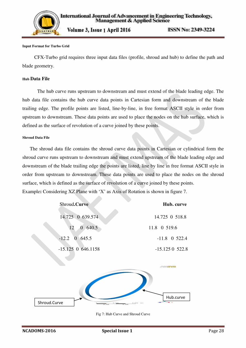
Example: Considering XZ Plane with ‘X’ as Axis of Rotation is shown in figure 7.

Shroud.Curve Hub. curve

14.725 0 639.574 14.725 0 518.8

12 0 640.5 11.8 0 519.6

-12.2 0 645.5 -11.8 0 522.4

-15.125 0 646.1158 -15.125 0 522.8

Fig 7: Hub Curve and Shroud Curve

Hub.curve

Shroud.Curve


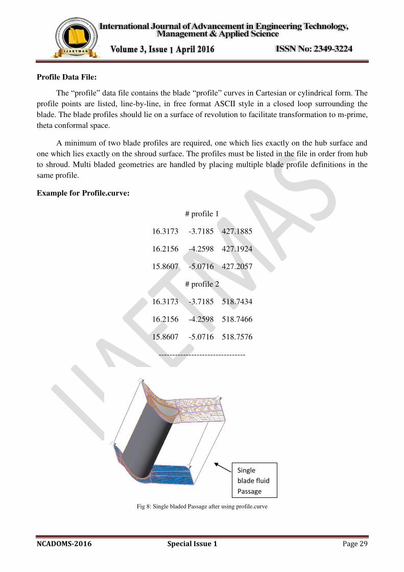
Profile Data File:

The “profile” data file contains the blade “profile” curves in Cartesian or cylindrical form. The

profile points are listed, line-by-line, in free format ASCII style in a closed loop surrounding the

blade. The blade profiles should lie on a surface of revolution to facilitate transformation to m-prime,

theta conformal space.

A minimum of two blade profiles are required, one which lies exactly on the hub surface and

one which lies exactly on the shroud surface. The profiles must be listed in the file in order from hub

to shroud. Multi bladed geometries are handled by placing multiple blade profile definitions in the

same profile.

Example for Profile.curve:

# profile 1

16.3173 -3.7185 427.1885

16.2156 -4.2598 427.1924

15.8607 -5.0716 427.2057

# profile 2

16.3173 -3.7185 518.7434

16.2156 -4.2598 518.7466

15.8607 -5.0716 518.7576

--------------------------------

Fig 8: Single bladed Passage after using profile.curve

Single

blade fluid

Passage


The first step is to check whether the blade profile data obtained from solid model is

intersecting hub and shroud curves or not. We use CFX-Turbogrid intersect option for this purpose.

Using this option, we have to see that blade profile must lie on the surface of revolution of hub and

shroud as shown in fig 8. Turbo grid intersecting capability can convert an existing set of blade

profiles that does not necessarily lie on the surface of revolution into one that can be used in a CFX-

Turbogrid template.

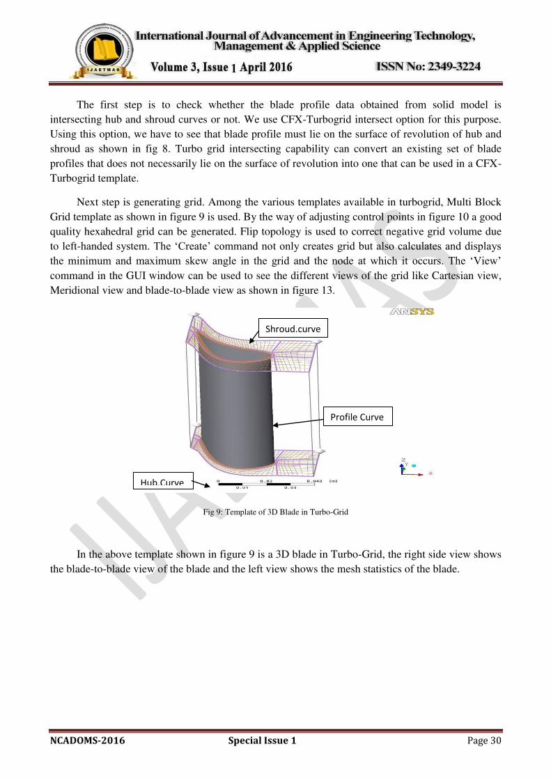
Next step is generating grid. Among the various templates available in turbogrid, Multi Block

Grid template as shown in figure 9 is used. By the way of adjusting control points in figure 10 a good

quality hexahedral grid can be generated. Flip topology is used to correct negative grid volume due

to left-handed system. The ‘Create’ command not only creates grid but also calculates and displays the minimum and maximum skew angle in the grid and the node at which it occurs. The ‘View’ command in the GUI window can be used to see the different views of the grid like Cartesian view,

Meridional view and blade-to-blade view as shown in figure 13.

Fig 9: Template of 3D Blade in Turbo-Grid

In the above template shown in figure 9 is a 3D blade in Turbo-Grid, the right side view shows

the blade-to-blade view of the blade and the left view shows the mesh statistics of the blade.

Profile Curve

Shroud.curve

Hub.Curve


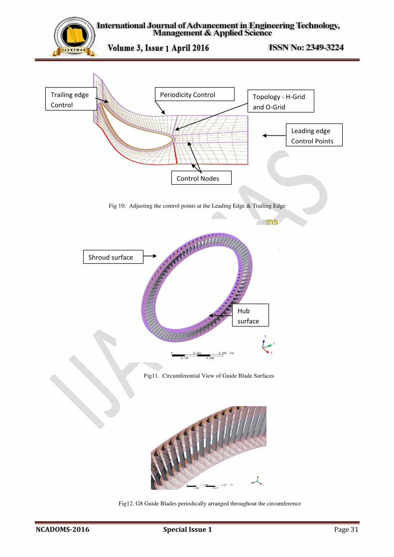
Fig 10: Adjusting the control points at the Leading Edge & Trailing Edge

Fig11. Circumferential View of Guide Blade Surfaces

Fig12. G8 Guide Blades periodically arranged throughout the circumference

Hub

surface

Shroud surface

Leading edge

Control Points

Trailing edge

Control

Periodicity Control

Control Nodes

Topology - H-Grid

and O-Grid


The mesh generated by adjusting the control points as shown in Figure 10 and correspondingly

Circumferential view of guide blade surfaces & Periodical arrangement of blades throughout the

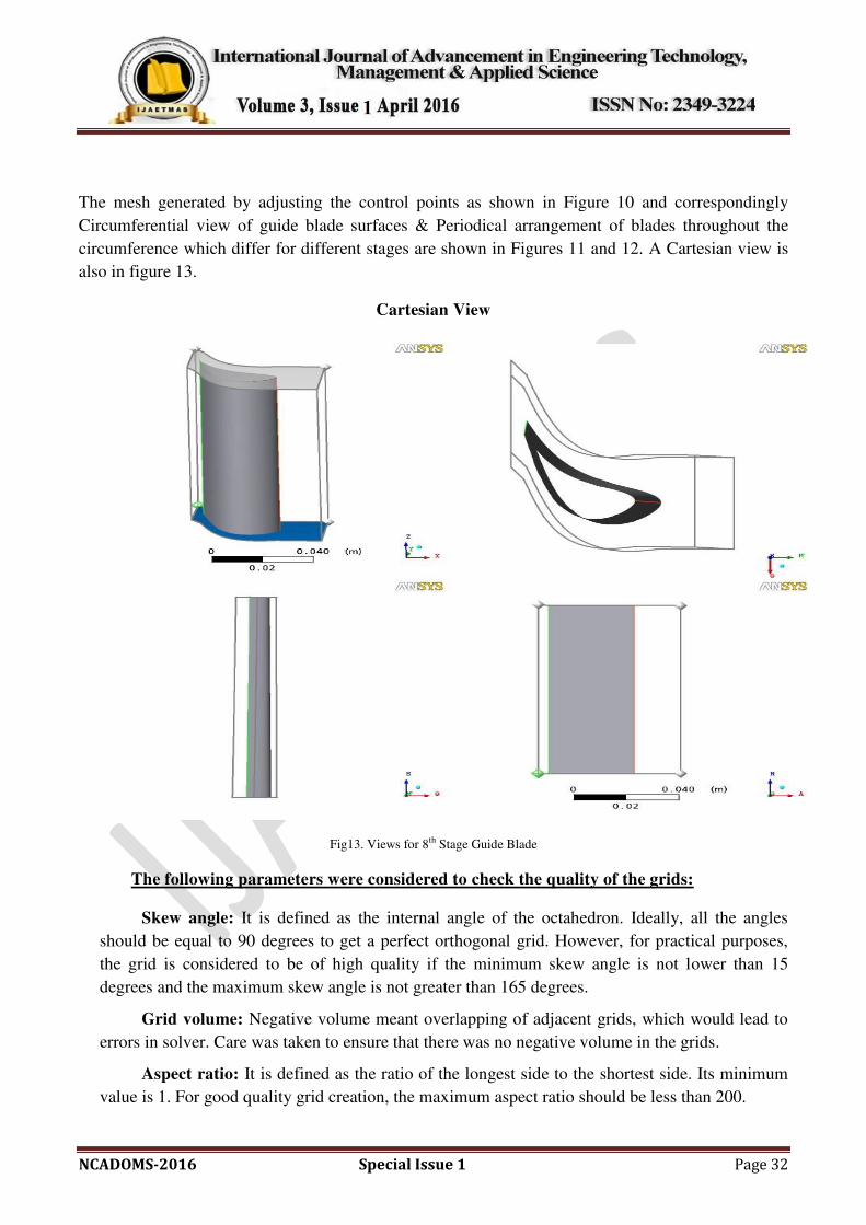
circumference which differ for different stages are shown in Figures 11 and 12. A Cartesian view is

also in figure 13.

Cartesian View

Fig13. Views for 8th Stage Guide Blade

The following parameters were considered to check the quality of the grids:

Skew angle: It is defined as the internal angle of the octahedron. Ideally, all the angles

should be equal to 90 degrees to get a perfect orthogonal grid. However, for practical purposes,

the grid is considered to be of high quality if the minimum skew angle is not lower than 15

degrees and the maximum skew angle is not greater than 165 degrees.

Grid volume: Negative volume meant overlapping of adjacent grids, which would lead to

errors in solver. Care was taken to ensure that there was no negative volume in the grids.

Aspect ratio: It is defined as the ratio of the longest side to the shortest side. Its minimum

value is 1. For good quality grid creation, the maximum aspect ratio should be less than 200.


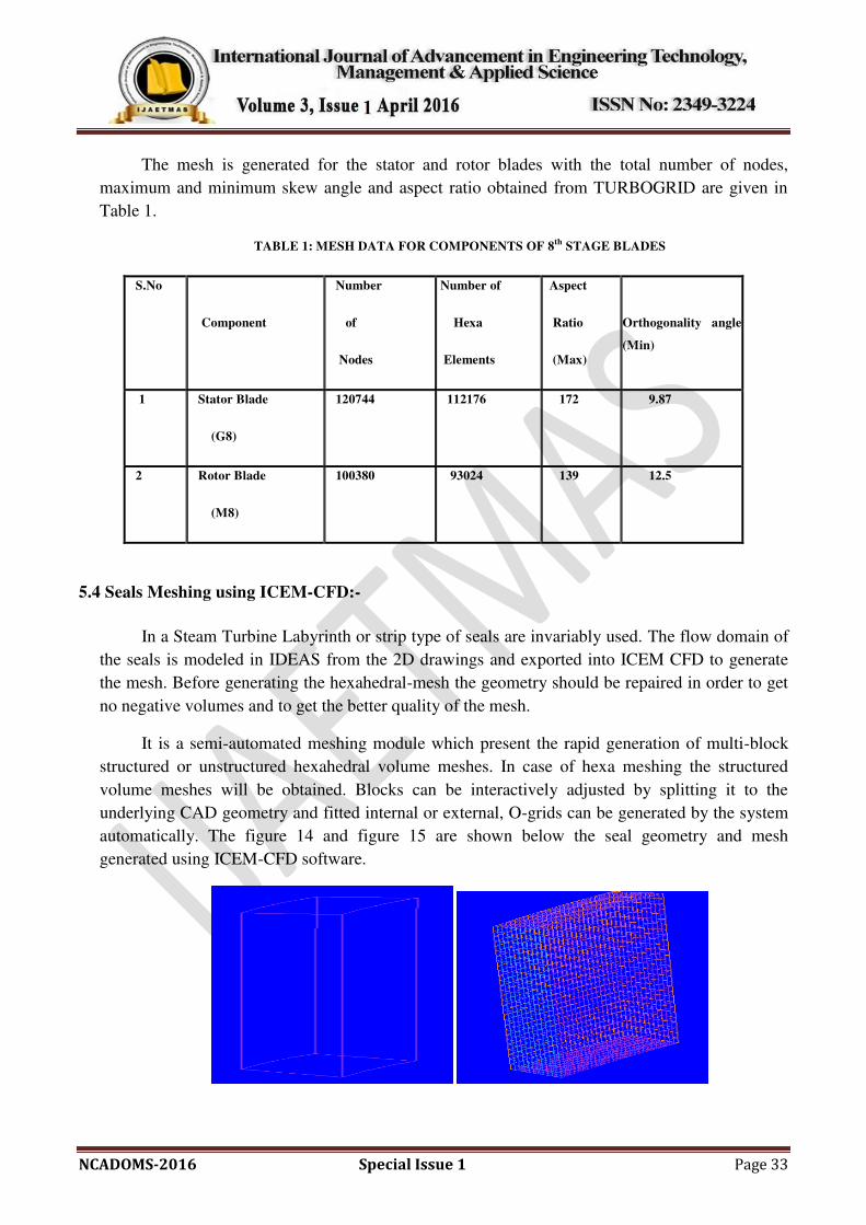
The mesh is generated for the stator and rotor blades with the total number of nodes,

maximum and minimum skew angle and aspect ratio obtained from TURBOGRID are given in

Table 1.

TABLE 1: MESH DATA FOR COMPONENTS OF 8th STAGE BLADES

S.No

Component

Number

of

Nodes

Number of

Hexa

Elements

Aspect

Ratio

(Max)

Orthogonality angle

(Min)

1 Stator Blade

(G8)

120744 112176 172 9.87

2 Rotor Blade

(M8)

100380 93024 139 12.5

5.4 Seals Meshing using ICEM-CFD:-

In a Steam Turbine Labyrinth or strip type of seals are invariably used. The flow domain of

the seals is modeled in IDEAS from the 2D drawings and exported into ICEM CFD to generate

the mesh. Before generating the hexahedral-mesh the geometry should be repaired in order to get

no negative volumes and to get the better quality of the mesh.

It is a semi-automated meshing module which present the rapid generation of multi-block

structured or unstructured hexahedral volume meshes. In case of hexa meshing the structured

volume meshes will be obtained. Blocks can be interactively adjusted by splitting it to the

underlying CAD geometry and fitted internal or external, O-grids can be generated by the system

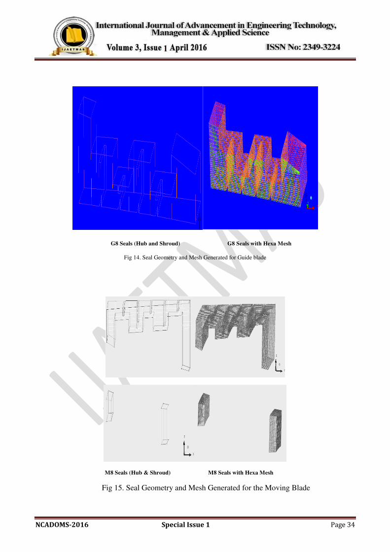
automatically. The figure 14 and figure 15 are shown below the seal geometry and mesh

generated using ICEM-CFD software.


G8 Seals (Hub and Shroud) G8 Seals with Hexa Mesh

Fig 14. Seal Geometry and Mesh Generated for Guide blade

M8 Seals (Hub & Shroud) M8 Seals with Hexa Mesh

Fig 15. Seal Geometry and Mesh Generated for the Moving Blade


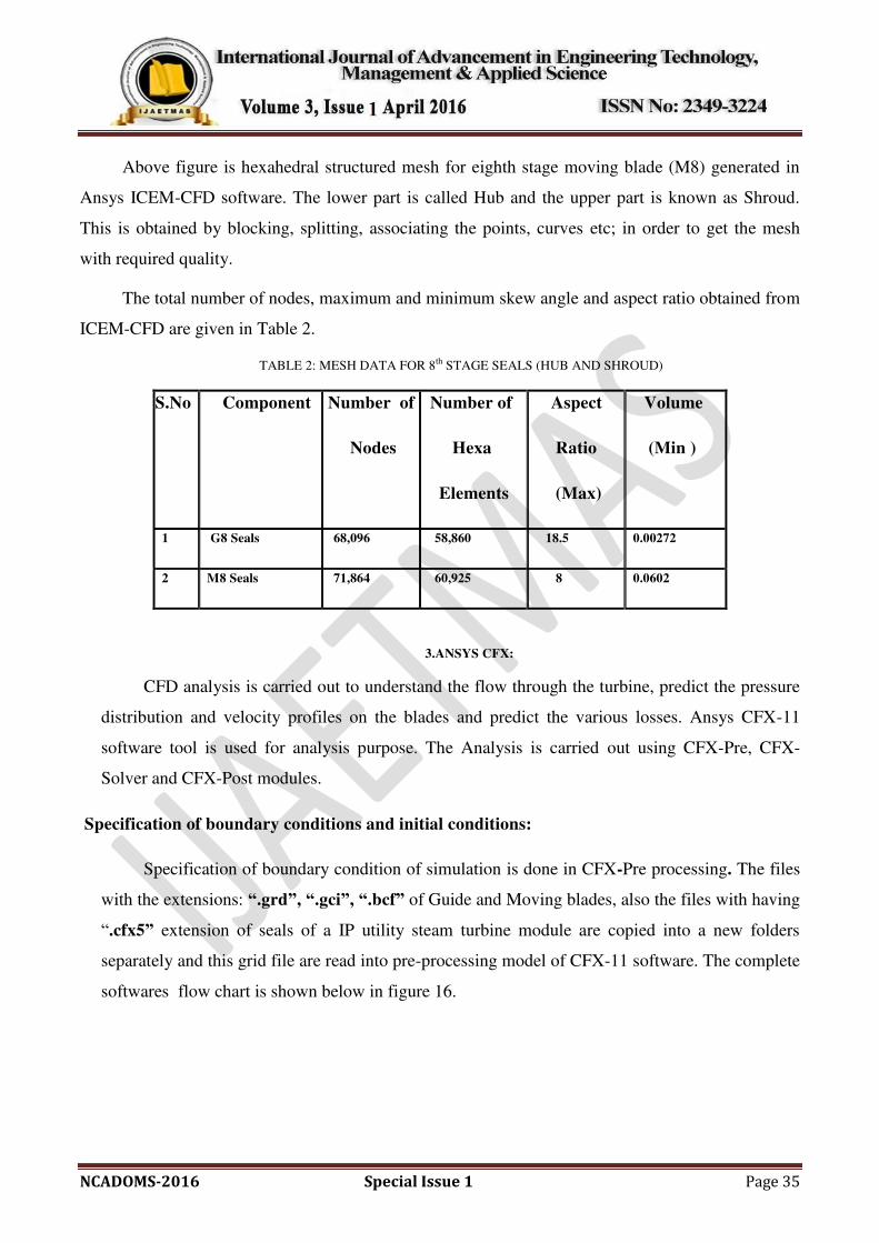
Above figure is hexahedral structured mesh for eighth stage moving blade (M8) generated in

Ansys ICEM-CFD software. The lower part is called Hub and the upper part is known as Shroud.

This is obtained by blocking, splitting, associating the points, curves etc; in order to get the mesh

with required quality.

The total number of nodes, maximum and minimum skew angle and aspect ratio obtained from

ICEM-CFD are given in Table 2.

TABLE 2: MESH DATA FOR 8th STAGE SEALS (HUB AND SHROUD)

S.No Component Number of

Nodes

Number of

Hexa

Elements

Aspect

Ratio

(Max)

Volume

(Min )

1 G8 Seals 68,096 58,860 18.5 0.00272

2 M8 Seals 71,864 60,925 8 0.0602

3.ANSYS CFX:

CFD analysis is carried out to understand the flow through the turbine, predict the pressure

distribution and velocity profiles on the blades and predict the various losses. Ansys CFX-11

software tool is used for analysis purpose. The Analysis is carried out using CFX-Pre, CFX-

Solver and CFX-Post modules.

Specification of boundary conditions and initial conditions:

Specification of boundary condition of simulation is done in CFX-Pre processing. The files

with the extensions: “.grd”, “.gci”, “.bcf” of Guide and Moving blades, also the files with having

“.cfx5” extension of seals of a IP utility steam turbine module are copied into a new folders

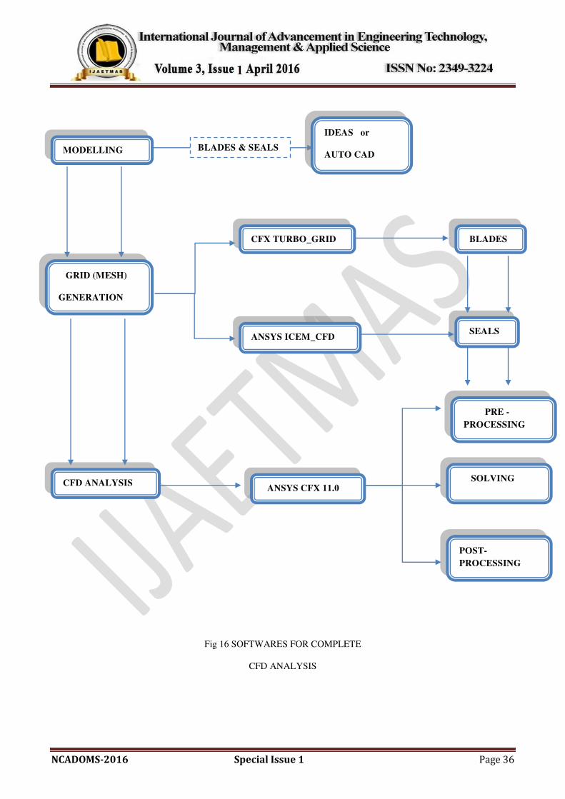
separately and this grid file are read into pre-processing model of CFX-11 software. The complete

softwares flow chart is shown below in figure 16.


Fig 16 SOFTWARES FOR COMPLETE

CFD ANALYSIS

MODELLING BLADES & SEALS

IDEAS or

AUTO CAD

GRID (MESH)

GENERATION

CFX TURBO_GRID

ANSYS ICEM_CFD

BLADES

SEALS

ANSYS CFX 11.0 CFD ANALYSIS

PRE -

PROCESSING

SOLVING

POST-

PROCESSING


III Result and Discussion

A. Results:

The analysis is carried out in two stages. First, initially the analysis is carried out for the 8th stage

and later combined analysis for all the 5 stages has been carried out. The stage analysis has been

carried out for the turbine stages with the constant mass flow and it consists of stator, rotor, and

seals. The various performance parameters like pressure, temperature distribution and velocity

profiles on the blades, isentropic efficiencies, Power have been computed using the CFX Macros and

with the help of Mollier Chart. As the eight stages consisting of Guide blade, Moving blade with a

stage interface between the blades is simulated, and the solution is obtained with high resolution

convergence up to 1e-5.The analysis is carried out with seals for 8th

stage. The results obtained are

discussed below:

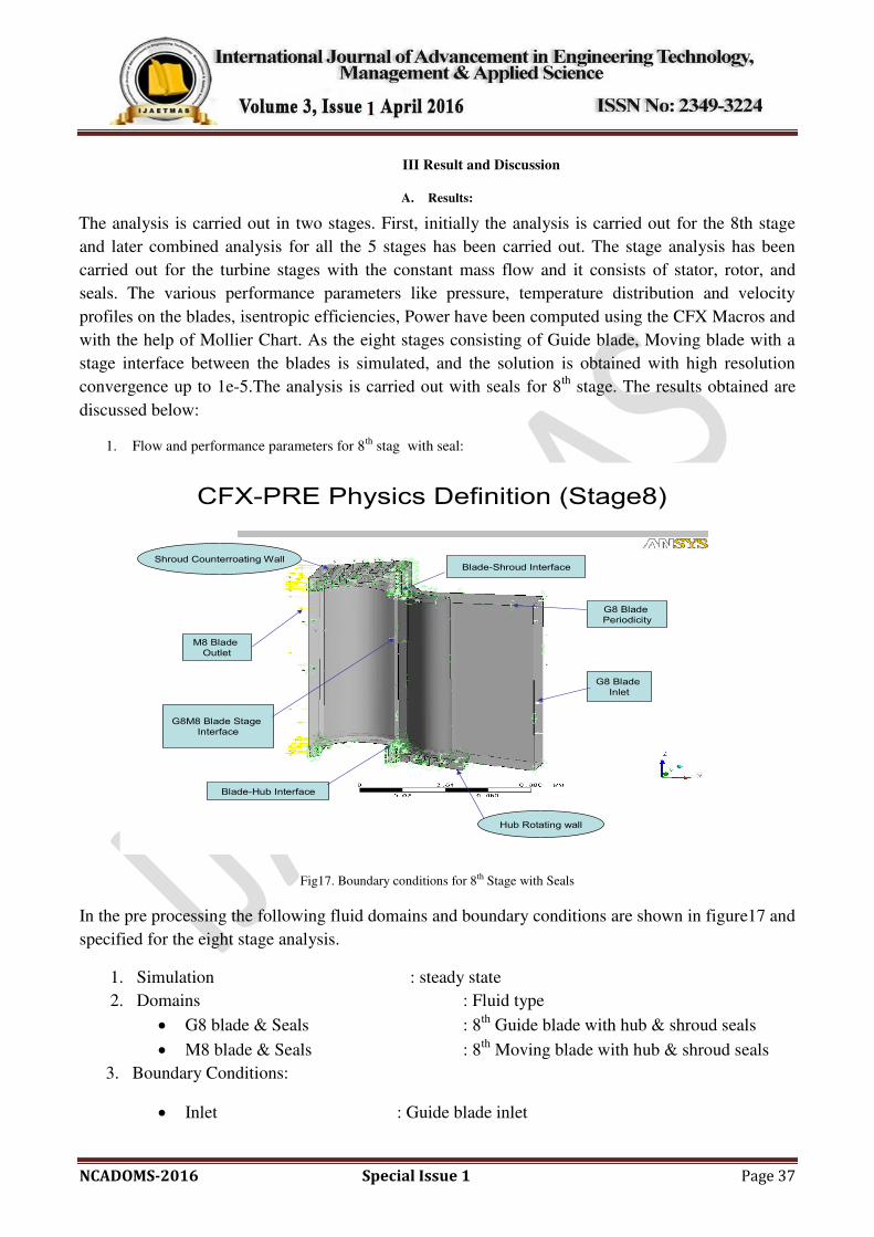
1. Flow and performance parameters for 8th

stag with seal:

CFX-PRE Physics Definition (Stage8)

G8 Guide Blade

Inlet

M8 Blade

Outlet

G8 Blade

Inlet

Hub Rotating wall

Shroud Counterroating Wall

G8M8 Blade Stage

Interface

G8 Blade

Periodicity

Blade-Shroud Interface

Blade-Hub Interface

Fig17. Boundary conditions for 8th Stage with Seals

In the pre processing the following fluid domains and boundary conditions are shown in figure17 and

specified for the eight stage analysis.

1. Simulation : steady state

2. Domains : Fluid type

G8 blade & Seals : 8th

Guide blade with hub & shroud seals

M8 blade & Seals : 8th

Moving blade with hub & shroud seals

3. Boundary Conditions:

Inlet : Guide blade inlet


Outlet : Moving blade outlet

Inlet Mass Flow : 1.199795 kg/sec

Inlet Static Temperature : 688.8 K

Wall : smooth

Outlet Static Pressure : 18.04 bar

Rotational Speed : -3000 rpm

Reference pressure : 0 bar

4. Fluid Properties:

Working Fluid : Steam5 (Dry steam)

Dynamic Viscosity : 25.0746e-6 Pa s

Thermal Conductivity : 0.0581942 W/m. ºc

5. Rotation Axis : X - Axis

6. Turbulence Model:

Turbulence Model : Standard k-Epsilon Model

Heat transfer Model : Total Energy

7. Interface between Guide and Moving Blade:

Type : Fluid -Fluid

Frame Change Option : Stage Interface(G8M8 Blade stage interface)

8. Pitch Change:

Option: Specified Pitch Angle

Pitch angle side 1: 2.465753

Pitch angle side 2: 3.130435

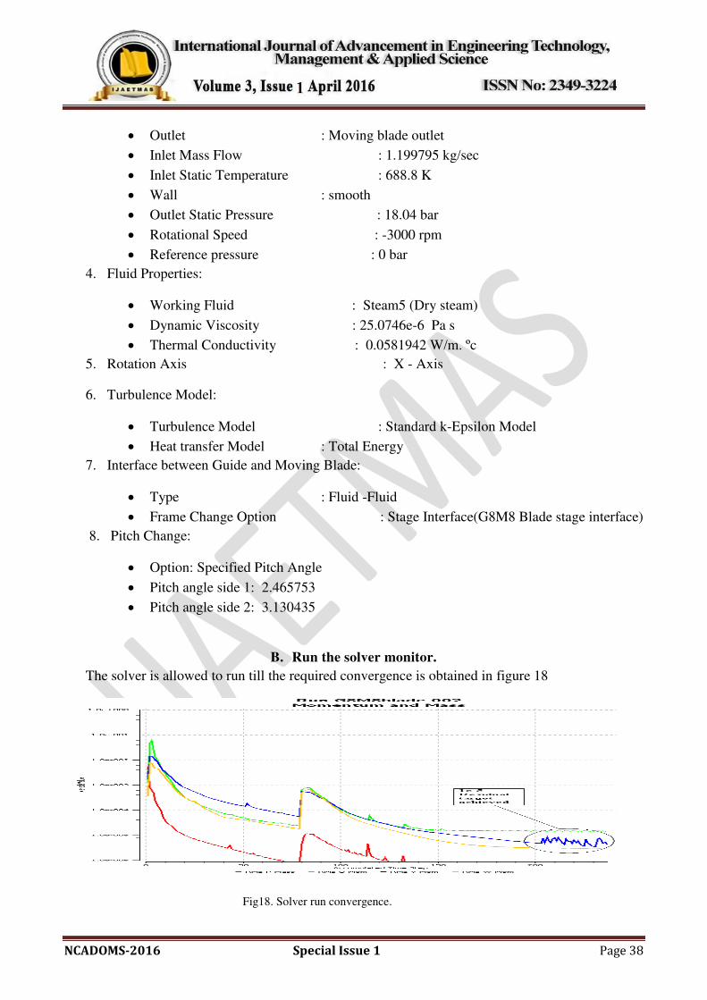
B. Run the solver monitor.

The solver is allowed to run till the required convergence is obtained in figure 18

Fig18. Solver run convergence.


C. POST PROCESSING:

1. Results which are obtained from the CFX macro for the Eighth stage User Input

Inlet Region G8 blade inlet

Outlet Region M8 blade outlet

Blade Row Region M8 blade Default

Reference Radius 0.575325 [m]

Number of Blade Rows 115

Machine Axis X

Rotation Speed -3000 [rev min^-1]

Gamma 1.3

Reference Pressure 0 [Pa]

2. Mass Averages

Quantity Inlet Outlet Ratio (Out/In)

Temperature 688.801 K 664.746 K 0.961184524456200

Total

Temperature 691.248 K 675.846 K 0.93.458010506430

Pressure 1.84207e+006 kg m^-1

s^-2

1.58472e+006 kg m^-1

s^-2 0.852351034358415

Total Pressure 1.96454e+006 kg m^-1

s^-2

1.61431e+006 kg m^-1

s^-2 0.895951241807446


3. Results

Torque (one blade row) -344.527 kg m^2 s^-2

Torque (all blades) -28584 kg m^2 s^-2

Power (all blades) -8.010974e+006 kg m^2 s^-3

Total-to-total isen. efficiency 0.912117

Total-to-static isen. efficiency 0.905874

Streamline and vector plots for various parameters have been given for better understanding of flow

through the stages.

The Pressure Contour shows the pressure variation across the stage. It is clear from the

Pressure Contour that the pressure drop occurs across the stage. The pressure is high at the beginning

of the stage, decreases across the stage and is low at the exit of the stage. The Pressure Contour is

useful to see the variation of pressure across the stage and modify the design if required to get

uniform pressure drop.

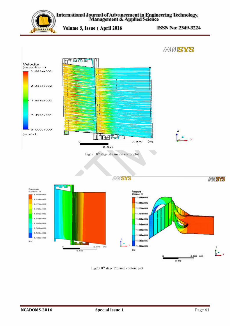
The Velocity Vector Plot shows the velocity variation across the stage is shown in figure 19.

It can be seen from the Velocity Contour Plot that the velocity is minimum at the entry of the guide

blade and reaches maximum at the exit of guide blade. Similarly for the moving blade also the

velocity is minimum at the entry and maximum at the throat. Thus the velocity changes for each

blade from minimum at entry to maximum at the throat.

The Velocity Streamline Plot is useful to note the streamline motion of the Steam through the

Stage. The Streamline motion is very useful to determine the proper flow of the steam through the

stage. The proper design of the stage should have the continuous streamline motion of the Steam

without any discontinuity.

The Velocity Vector Plot is useful to draw the velocity triangles of the stage. The power

output of the stage depends upon the velocity triangles. Thus the velocity vector is an important plot

to decide the design efficiency of the stage. It is very important design the stage to get the required

power output so the velocity vector plot is good indicator of the design of the stage.

The Pressure Contour, Mach number Contour, Velocity Streamline and Velocity Vector Plots

for 8th

Stage with seals are shown below.

4. Plots for 8th

Stage with Hub & Shroud seals:


Fig19. 8th stage streamline vector plot

Fig20. 8th stage Pressure contour plot


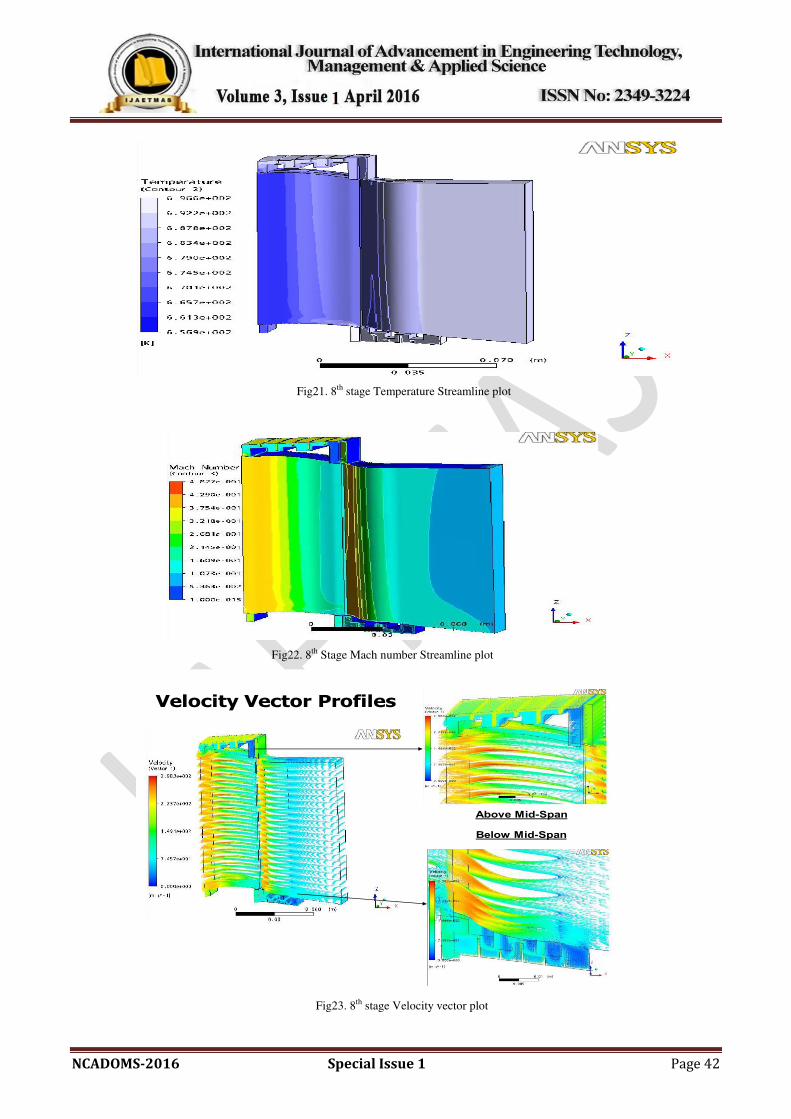
Fig21. 8th stage Temperature Streamline plot

Fig22. 8th Stage Mach number Streamline plot

Velocity Vector Profiles

Above Mid-Span

Below Mid-Span

Fig23. 8th stage Velocity vector plot


5. Discussions:

Streamline, vector and contour plots for various parameters have been given for better

understanding of the flow through the stages.

The variation of pressure across the stage is seen in Fig 20, it is a pressure contour plot

which is a series of lines linking points with equal values of a given variable pressure. It is shown

in the figure that the pressure goes on decreasing from entry to exit of the stage. At the entrance

the maximum of 18.564 bar is observed and a minimum of 14.65 bar is obtained at the exit is

obtained.

The Contour plot for the variation of temperature across the 8th

stage is shown in Fig 21.

From the figure it is clear that the temperature is decreasing from the entry to the exit. At the

entrance the temperature is maximum around 696.6 K, and at the exit the temperature is

minimum of 656.9 K.

Fig 22 shows the variation of Mach number across the 8th

stage with seals. From the

figure it is obvious that Mach number is increasing from the entry to exit and minimum Mach

number of the order of 0.05363 occurred at the entrance of the guide blade and a maximum of

0.4827 is occurred at the interface of the guide blade and moving blade.

Fig 23 shows the variation of the velocity across the eighth stage. This vector plot, which is

a collection of vectors drawn to show the direction and magnitude of a vector variable on a

collection of points are defined by arrows. From the figure it is obvious that the velocity is

minimum at the entrance which is of 7.51 m/sec and maximum at the interface and at the exit of

the stage which is around 298.8 m/sec.

6. Comparison of CFD values and 2D Values:

The CFD analysis results are compared with 2D program output. The program output is

verified experimentally. The comparison chart of 2D values and CFD values for 8th

stage are

shown in the table 3. The values obtained show that the CFD values are closer to 2D program and

are within the acceptable limits.

Table3. Comparison of CFD values and 2D values.

STAGE 8 WITH SEALS

Description Unit 2D value CFD Value

Temp inlet K 688.8 688.801

Temp outlet K 667.1 664.746


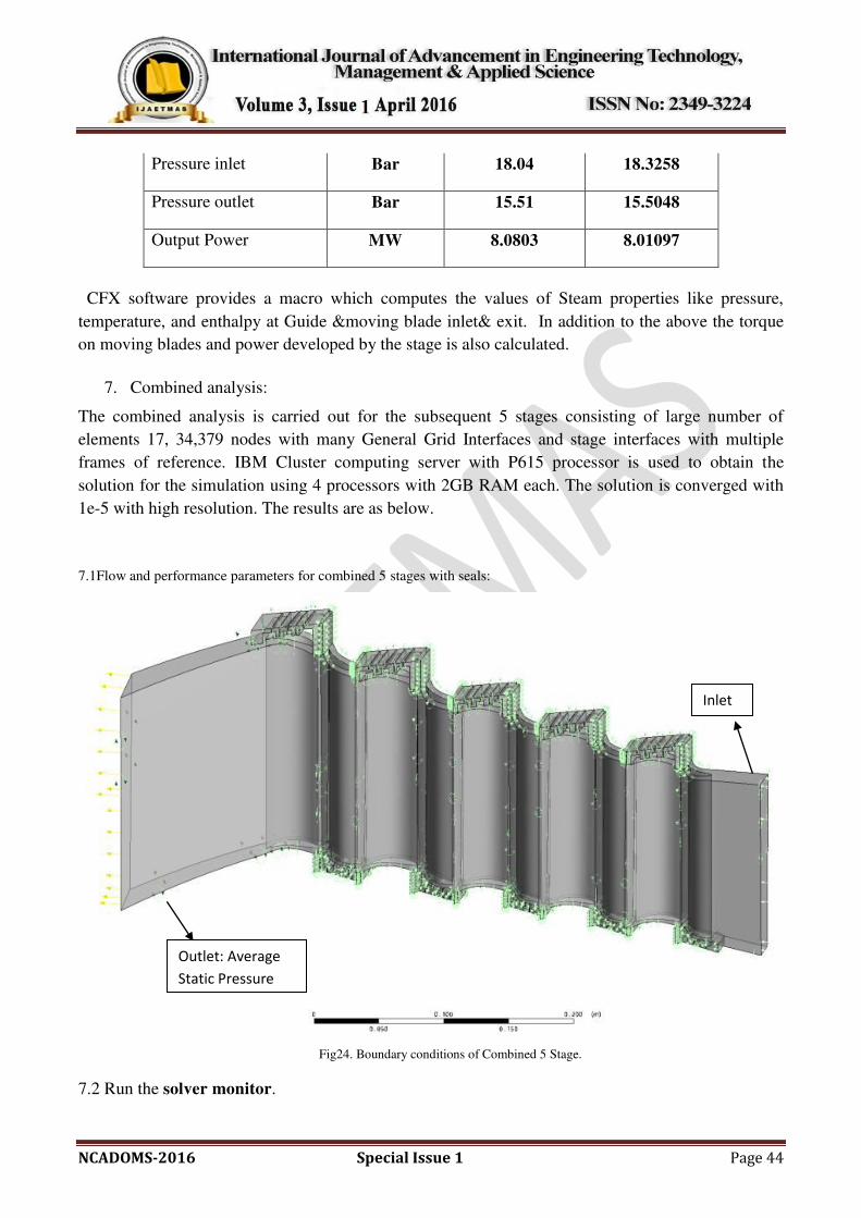
Pressure inlet Bar 18.04 18.3258

Pressure outlet Bar 15.51 15.5048

Output Power MW 8.0803 8.01097

CFX software provides a macro which computes the values of Steam properties like pressure,

temperature, and enthalpy at Guide &moving blade inlet& exit. In addition to the above the torque

on moving blades and power developed by the stage is also calculated.

7. Combined analysis:

The combined analysis is carried out for the subsequent 5 stages consisting of large number of

elements 17, 34,379 nodes with many General Grid Interfaces and stage interfaces with multiple

frames of reference. IBM Cluster computing server with P615 processor is used to obtain the

solution for the simulation using 4 processors with 2GB RAM each. The solution is converged with

1e-5 with high resolution. The results are as below.

7.1Flow and performance parameters for combined 5 stages with seals:

Fig24. Boundary conditions of Combined 5 Stage.

7.2 Run the solver monitor.

Outlet: Average

Static Pressure

Inlet


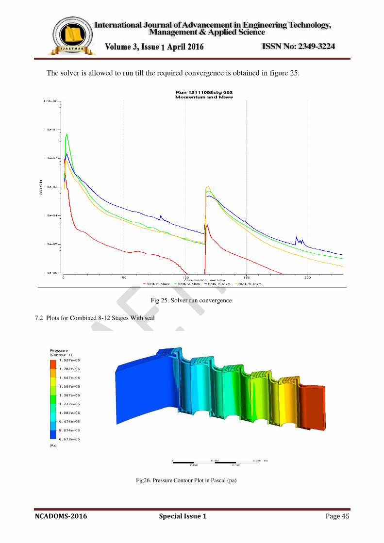
The solver is allowed to run till the required convergence is obtained in figure 25.

Fig 25. Solver run convergence.

7.2 Plots for Combined 8-12 Stages With seal

Fig26. Pressure Contour Plot in Pascal (pa)


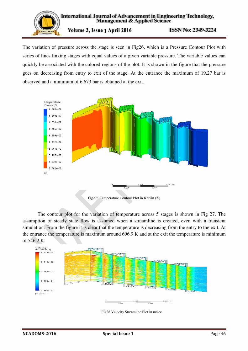
The variation of pressure across the stage is seen in Fig26, which is a Pressure Contour Plot with

series of lines linking stages with equal values of a given variable pressure. The variable values can

quickly be associated with the colored regions of the plot. It is shown in the figure that the pressure

goes on decreasing from entry to exit of the stage. At the entrance the maximum of 19.27 bar is

observed and a minimum of 6.673 bar is obtained at the exit.

Fig27: Temperature Contour Plot in Kelvin (K)

The contour plot for the variation of temperature across 5 stages is shown in Fig 27. The

assumption of steady state flow is assumed when a streamline is created, even with a transient

simulation. From the figure it is clear that the temperature is decreasing from the entry to the exit. At

the entrance the temperature is maximum around 696.9 K and at the exit the temperature is minimum

of 546.2 K.

Fig28 Velocity Streamline Plot in m/sec


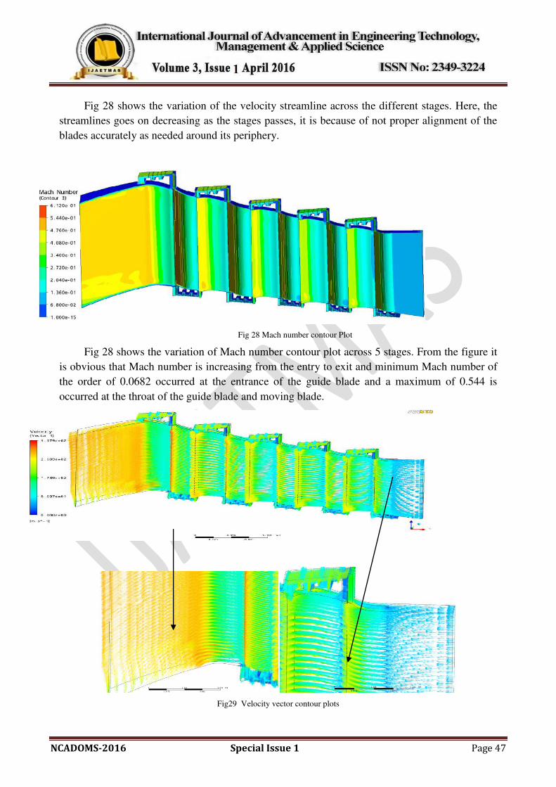
Fig 28 shows the variation of the velocity streamline across the different stages. Here, the

streamlines goes on decreasing as the stages passes, it is because of not proper alignment of the

blades accurately as needed around its periphery.

Fig 28 Mach number contour Plot

Fig 28 shows the variation of Mach number contour plot across 5 stages. From the figure it

is obvious that Mach number is increasing from the entry to exit and minimum Mach number of

the order of 0.0682 occurred at the entrance of the guide blade and a maximum of 0.544 is

occurred at the throat of the guide blade and moving blade.

Fig29 Velocity vector contour plots


Above Figure 29 shows the variation of the velocity across the each stage in the combined

5 stages. This a vector plot, which is a collection of vectors drawn to show the direction and

magnitude of a vector variable on a collection of points and are defined by a location. From the

figure it is obvious that the velocity is minimum at the entrance which is of 86.97 m/sec and

maximum at the throat of the stage which is around 347.9 m/sec.

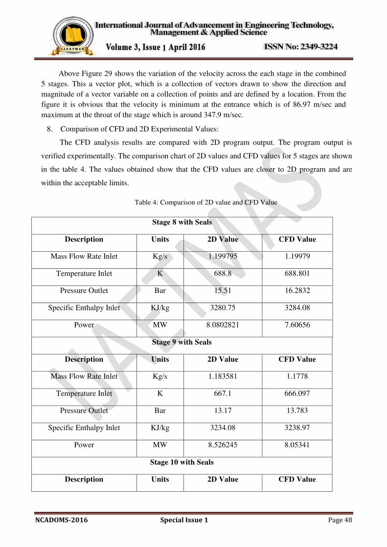
8. Comparison of CFD and 2D Experimental Values:

The CFD analysis results are compared with 2D program output. The program output is

verified experimentally. The comparison chart of 2D values and CFD values for 5 stages are shown

in the table 4. The values obtained show that the CFD values are closer to 2D program and are

within the acceptable limits.

Table 4: Comparison of 2D value and CFD Value

Stage 8 with Seals

Description Units 2D Value CFD Value

Mass Flow Rate Inlet Kg/s 1.199795 1.19979

Temperature Inlet K 688.8 688.801

Pressure Outlet Bar 15.51 16.2832

Specific Enthalpy Inlet KJ/kg 3280.75 3284.08

Power MW 8.0802821 7.60656

Stage 9 with Seals






Power MW 8.526245 8.05341

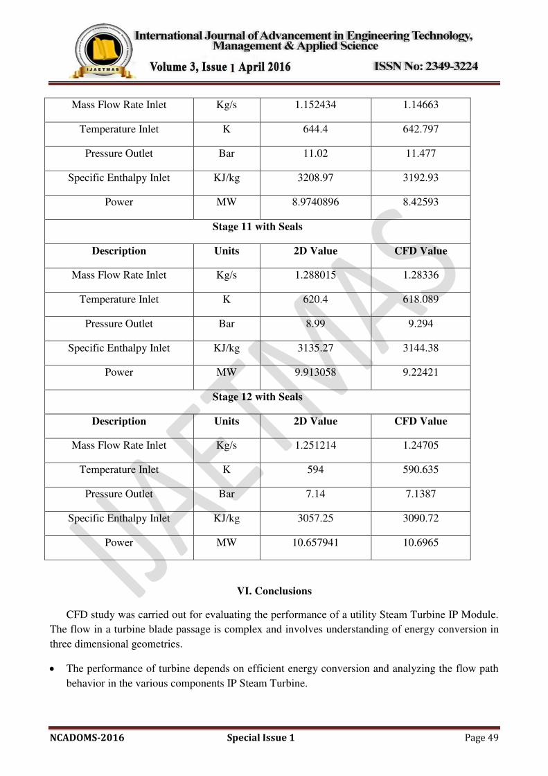
Stage 10 with Seals







Power MW 8.9740896 8.42593

Stage 11 with Seals






Power MW 9.913058 9.22421

Stage 12 with Seals



Temperature Inlet K 594 590.635



Power MW 10.657941 10.6965

VI. Conclusions

CFD study was carried out for evaluating the performance of a utility Steam Turbine IP Module.

The flow in a turbine blade passage is complex and involves understanding of energy conversion in

three dimensional geometries.

The performance of turbine depends on efficient energy conversion and analyzing the flow path

behavior in the various components IP Steam Turbine.


The CFD analysis of the turbine flow path helps in analyzing the flow and performance

parameters and their effects on performance parameters like temperature, pressure and Power

output.

The Intermediate Pressure turbine consisting of 5 stages with cylindrical profiles used

for stationary and moving blades. The blades are also designed with sealing strips between stationary

parts and rotating parts to reduce leakage losses. The flow path of the turbine with blades and seals is

modeled and meshed using different software’s like IDEAS, ANSYS-ICEMCFD, ANSYS-TURBO-

GRID, etc. The mesh for the blade region is generated separately with ANSYS-TURBO-GRID and

mesh for the seals are generated from ANSYS-ICEM-CFD and attached by General Grid Interface.

The analysis is carried out for a single stage initially and subsequently for all the combined 5

stages. The combined analysis consists of large number of elements 17,34,379 nodes with many

General Grid Interfaces and stage interfaces between multiple frames of reference. IBM Cluster

computing server with P615 processor is used to obtain the solution using 4 processors with 2GB

RAM each. The solution is converged with 1e-5 with high resolution.

The results are analyzed for mass flow rates, temperature and pressure distributions on blades,

power developed by stage and isentropic efficiency of the stage. The results are compared with Two-

Dimensional program validated by experimentally and found to be in agreement with the 2D

analysis. The CFD analysis of the Intermediate Pressure turbine module has helped in predicting the

turbine performance and comparing with experimentally verified values.

V. References

1. C.W. Haldeman , R.M. Mathison; Aerodynamic and Heat Flux Measurements in a Single-

Stage Fully Cooled Turbine – Part II, Journal of Turbomachinery, vol. 130/021016, April 2008.

2. X.Yan, T.Takinuka; Aerodynamic Design Model Test and CFD Analysis for a Multistage

Axial Helium Compressor, Journal of Turbomachinery, ASME paper,Vol. 130/031018, July

2008.

3. Arun K.Saha, Sumanta Acharya, Computations of Turbulent Flow and Heat Tansfer Through

a Three-Dimensional Nonaxisymmetric Blade Passage, Journal of Turbomachinery, ASME

paper, Vol. 130/031008, July 2008

4. Horloc, J.H., The Thermodynamics Efficiency of the Field Cycle , ASME paper, Vol. no.

57.A.44, 1957.

5. Computational Fluid Dynamics, the basics with applications - John D. Anderson. Jr

6. Fluid Mechanics and hydraulic machines - Dr. R. K. Bansal

7. Numerical heat transfer and Fluid Flow - Suhas V. Patankar

8. Steam Turbine Theory and Practice - W. J. Kearton

Websites:

www.cfd-online.com


Documents

CFD ANALYSIS Of COMBINED 8-12 STAGES Of · PDF fileCFD ANALYSIS Of COMBINED 8-12 STAGES Of INTERMIDIATE PRESSURE STEAM TURBINE ... I. Introduction %+ ... The blade of the Utility IP