CFD analysis of the flow in the near wake of a generic PWR mixing grid

Annals of Nuclear Energy xxx (2014) xxx–xxx

Contents lists available at ScienceDirect

Annals of Nuclear Energy

journal homepage: www.elsevier .com/locate /anucene

CFD analysis of the flow in the near wake of a generic PWR mixing grid

http://dx.doi.org/10.1016/j.anucene.2014.08.0040306-4549/� 2014 Elsevier Ltd. All rights reserved.

⇑ Corresponding author.E-mail address: [email protected] (U. Bieder).

Please cite this article in press as: Bieder, U., et al. CFD analysis of the flow in the near wake of a generic PWR mixing grid. Ann. Nucl. Energy (2014)dx.doi.org/10.1016/j.anucene.2014.08.004

Ulrich Bieder a,⇑, François Falk b, Gauthier Fauchet a

a CEA-Saclay, DEN, DM2S, STMF, F-91191 Gif sur Yvette, Franceb CEA-Grenoble, DEN, DTN, STRI, F-38047 Grenoble, France

a r t i c l e i n f o

Article history:Received 25 April 2014Accepted 3 August 2014Available online xxxx

Keywords:Pressurized Water Reactor (PWR)Mixing gridCFDTrio_UStrong scaling

a b s t r a c t

The flow in fuel assemblies of PWRs with mixing grids has been analyzed with CFD calculations bynumerous authors. The comparison between calculation and experiment has often shown an insensitivityof the calculated cross flow velocity on the turbulence modeling. The study presented here was carriedout to confirm this result. The comparison between measurements in the AGATE facility (5 � 5 tubebundle) and Trio_U calculations with a linear eddy viscosity turbulence model (k–e) and Large EddySimulations (LES) is presented.

The AGATE experiments have originally not been designed for CFD validation but to characterize dif-ferent types of mixing grids. Nevertheless, the quality of the experimental data allows the quantitativecomparison between measurement and calculation.

The test section of the AGATE facility has been discretized for the LES calculation on 300 million controlvolumes by using a staggered grid approach on tetrahedral meshes. 20 days of CPU on 4600 cores of theHPC machine CURIE of the TGCC was necessary to calculate the statistics of the turbulent flow, in partic-ular the mean velocity and the RMS of the turbulent fluctuations. The parallelism of Trio_U was tested upto 10,000 processor cores using strong scaling and has shown a good efficiency up to about 6000 cores,i.e., 40,000 control volumes per core.

For various distances from the mixing grid, calculated horizontal profiles of the cross flow velocity andof the axial velocity are compared to measurements. It seems that the flow patterns directly downstreamof the grid are insensitive to the used turbulence model. Inertia forces related to the geometry of the mix-ing vanes are dominant in this region. Thus, the application of turbulence models should not be testedclose to mixing grids.

� 2014 Elsevier Ltd. All rights reserved.

1. Introduction

In the last years a tremendous work has been done to predictwith CFD codes the fluid mixing in fuel assemblies with mixinggrids. Recently, the OCDE/NEA has initiated an international CFDbenchmark which was associated to the MATHIS_H experimentsof KAERI (Lee et al., 2012; Smith et al., 2013). This benchmark wasfocused on the mixing close to the mixing grid that is on an axial dis-tance of the first four hydraulic diameters (dh) downstream of thegrid. Results at 8dh are discussed but are not part of the benchmarkanalysis. The benchmark has shown an insensitivity of the calcu-lated velocity profiles on the turbulence modelling. This surprisingresult is verified in this paper by analyzing the swirling flow inthe near wake of a generic prototype mixing grid by both, RANSmodelling (Reynolds Averaged Navier–Stokes) based on the lineareddy viscosity concept (k–e) and LES (Large Eddy Simulation).

In the experimental set-up of the MATHIS_H experiment, themeasurements have been performed very close to the test channeloutlet. Bieder (2012) has shown that an influence of the outlet ple-num on the mixing in the wake of the grid cannot be excluded.Thus, for the study presented here, experiments were analyzedwhere outlet effects on the velocity profiles are not present. Theseexperiments have been performed at CEA between 1991 and 2001in the AGATE test facility (Falk and Mempontail, 1998).

2. The AGATE experiments

Mixing grids are designed by nuclear power plant vendors tocreate a specific coolant mixing behavior in the fuel assembly.The mixing grid acts as momentum source which increases the tur-bulence level and guides the transverse flow pattern as a functionof the specific vane design. More than 30 mixing grids have beenanalyzed and characterized in the AGATE facility (Falk andMempontail, 1998).

, http://

http://dx.doi.org/10.1016/j.anucene.2014.08.004

mailto:[email protected]


http://www.sciencedirect.com/science/journal/03064549

http://www.elsevier.com/locate/anucene



Table 1Geometrical parameters of the test section.

Rod diameter 9.5 mmRod pitch 12.6 mmdh of a central sub channel 11.78 mmChannel length 1200 mmMeasuring window length 800 mm

Table 2Quality of the AGATE measurements.

Positioning of the rods 0.1 mmPositioning of the velocity samples 0.05 mmEllipsoidal sample volume 0.6 mm * 0.06 mm; V = 0.01 mm3

Automatic displacement of the samples <0.03 mm in all axisFlow rate control ±0.5% with a RMS� 1%.Inflow temperature control ±0.1 KAxial velocity measurement ±0.1%Cross flow measurement ±0.75%

2 U. Bieder et al. / Annals of Nuclear Energy xxx (2014) xxx–xxx

The test section consists of a 5 � 5 rod bundle and a mixing grid,which are placed within a metallic channel of a quadratic cross

Side view of the mixing grid

Fig. 1. Side view and top view

Components of the measured velocity

Fig. 2. Measuring direction in the rod bundle (left)

Please cite this article in press as: Bieder, U., et al. CFD analysis of the flow in thdx.doi.org/10.1016/j.anucene.2014.08.004

section with a length of 66.1 mm of each side. One non-reflectingglass window allows LDA measurements which are placed onone channel side. The geometrical parameters shown in Table 1characterize the test section:

The water circuit is pressurized at 2 bars. A pump of 11 kW isdriving the flow which can attain a Reynolds Number of 2.5 * 105,a value which is only about 50% below that of a PWR at nominalconditions (5.0 * 105).The quality of the measured velocity is influ-enced by various factors which are summarized in Table 2 andquantified for the AGATE experiments.

For there is only one glass window in the experimental facility,the Laser Doppler Anemometry (LDA) measurement of the twocross flow velocities require two successive measuring campaigns.In order to simplify the measuring procedure, the velocitymeasurements are realized at constant axial locations. Themeasurements performed at a constant axial location are shownschematically in Fig. 2.

For each axial location, 21 velocity points are measured per sub-channel for the first horizontal direction (e.g., the red direction ofFig. 2). After passing through all six sub-channels of the rod bundle,the LDA system is switched axially to the next elevation. When allaxial elevations have been analyzed, the experiment is stopped;

Top view of the grid

of a generic mixing grid.

Measuring points in a sub-channel

and measuring points per sub channel (right).

e near wake of a generic PWR mixing grid. Ann. Nucl. Energy (2014), http://



Fig. 3. Typical form of horizontal flow pattern imposed by the mixing grids in theAGATE facility.

Table 3

U. Bieder et al. / Annals of Nuclear Energy xxx (2014) xxx–xxx 3

the mixing grid is dismount, turned by 90� and remounted at thesame axial position. Then, the experiment is repeated for the otherhorizontal direction (the green direction in Fig. 2) for the sameaxial locations. Due to this procedure, the axial velocity is mea-sured twice at nine points in the center of a sub channel (bluepoints in Fig. 2). These double values of the axial velocity are usedto evaluate the reproducibility of the measuring campaign.

For each location in the measuring plane, the instantaneousfluid velocity components are measured simultaneously with theLDA system at a frequency of about 1 kHz. The collecting periodto attain temporal mean values varies between 10 and 250 s,depending on the temporal convergence of the signal. Only con-verged mean values are used for the subsequent analysis. Due tothe measuring procedure from the channel side, the complete crossflow velocity vectors can only be reconstructed in the center of thesub channels (blue points in Fig. 2). For the other measuring points,only one component of the vector is available and large parts of thesub channel are not accessible by the laser beam.

The mixing vane arrangement shown in Fig. 1 typically causes adiagonal flow at 45� in the near wake of the mixing grid as shownin Fig. 3.

The thermal–hydraulic conditions of the analyzed test and thecorresponding physical properties are given in Table 3. The mixinggrid was placed 50 hydraulic diameters (dh) downstream of thetest section entrance. The LDA measurements have been done at15 axial distances from the mixing grid upper edge namely from�9.3dh to 51dh.

Test conditions and physical properties.

Density q 990.7 kg/m3

Viscosity l 6.528 * 10�4 Pa sTemperature T 40 �CMean axial velocity uz 5.375 m/sReynolds number Re 96,000 –

Table 4LES numerical scheme.

General Mesh Tetrahedral meshDiscretization P0 + P1 for: P P1NC for: U

Time scheme Runge–Kutta 3rd order explicit

Spatial Convection 2nd order centeredDiscretisation Diffusion 2nd order centered

Pressure solver PETSc GCP with SSOR preconditioningWall law Law of Reichhardt

Turbulence LES WALE

Table 5RANS numerical scheme.

General Mesh Tetrahedral meshDiscretization P0 + P1 for: P P1NC for: U

Time scheme Euler backward 1rd order implicit

Spatial Convection 2nd order upwindDiscretisation Diffusion 2nd order centred

Pressure solver PETSc GCP with SSOR preconditioningWall law Law of Reichhardt

Turbulence RANS k–e

3. Method

3.1. The CFD code Trio_U

Trio_U is a CFD code for unsteady, low Mach number, turbulentflows. The code is especially designed for industrial CFDcalculations on structured (parallelepipeds) and non-structured(tetrahedrons) grids of several hundreds of millions of processorcores (Trio_U, 2006). The platform independent code, developedat CEA, is based on an object oriented, intrinsically parallelapproach and is coded in C++ (Calvin et al., 2002). The flexible codestructure allows the user to choose a suitable discretizationmethod and to combine various appropriate physical models,including different treatments of turbulence. Several convectionand time marching schemes as well as a wide range of boundaryconditions are available. The code has been run successfully onmassively parallel computers with up to 10,000 processor coreswithout a significant reduction of the overall performance.

A hybrid Finite Volume Element discretization method (FVE) isimplemented for tetrahedral grids (Ducros et al., 2010). Thismethod approximates a continuous problem by a discrete solutionin the space of the finite elements by maintaining the balancenotation of finite volumes. In Trio_U, the main unknowns as veloc-ity and temperature are located in the center of the faces of the tet-rahedral element leading to a P1 non-conforming discretization(P1NC). Thus, the number of control volumes for the momentumand scalar conservation is approximately two times the numberof elements. The pressure is discretized in both the center (P0)and the vertices (P1) of an element. The resulting staggered mesharrangement improves the velocity/pressure coupling (Fortin,2006). The SOLA velocity projection method of Hirt et al. (1975)is used to assure the mass conservation.

3.2. The numerical schemes of the analysis

The AGATE experiment was analyzed by two types of turbu-lence modeling: LES and RANS (k–e). For LES, an explicit 3rd order


Runge–Kutta time marching scheme was used to solve theunsteady momentum equations, combined with a pressure projec-tion method for mass conservation (Hirt et al., 1975). The convec-tion term is discretized by a 2nd order centered scheme developedby Kuzmin and Turek, 2004 for scalar transport. This scheme hasbeen extended by Fortin (2006) to momentum transport. Addi-tional information on the LES numerical scheme is summarizedin Table 4.




Tetrahedrization of one hexahedral cell Meshing of the whole domain in 34992 tetrahedrons

Fig. 4. Tetrahedrization method and example of a meshing with symmetric expansion.

Table 6Result of strong scaling for the first time step.

Processor cores Iterations to convergence CPU temps in s Tetras/core

500 5733 181.4 213,2601000 5735 82.9 100,6632000 6019 43.6 50,3314000 5877 22.1 25,1656000 6018 16.2 16,7778000 6042 13.2 12,58310,000 5979 11.9 10,066

Fig. 5. Measured speed-up when increasing the number of processor cores.

Fig. 6. Time spent in the operators to construct the second member.

Periodic box

Mixing grid

Test section

Fig. 7. CAD model of the test section.


For RANS calculation, the 1st order Euler backward time march-ing scheme was used to solve the steady momentum equations. Afully implicit velocity projection method is used to assure the massconservation. The stability of this scheme has been demonstratedby Guermond and Quartapelle, 1998. A MUSCL type 2nd orderupwind scheme is used to discretise the convection term. Thenumerical scheme for RANS calculations is given in Table 5. Moredetailed information on the implicit numerical scheme and thesolution method is given by Ducros et al. (2010).

3.3. The parallel efficiency

As already mentioned, the solution method for LES calculationsof Trio_U is based on the pressure projection method of Hirt et al.(1975). The code spends around 60–80% of the calculation time in


the pressure solver in which a large system of coupled linear equa-tions is solved. A test case has been selected to test especially theparallel efficiency of the pressure solver and which measuressimultaneously the times to construct the second member.





A stagnant flow in the presence of a non-linear source term issimulated for a cube of 1 m length in each direction. The flow isassumed to be incompressible (q = constant). The calculationis based on the following set of equations:

3.3.1. Momentum equations

@~u@tþ~u � ~r~u ¼ � 1

q~rpþ ~r � m ~r~u

� �þ~S

3.3.2. Mass conservation

~r �~u ¼ 0

3.3.3. Initial conditions

~uðt ¼ 0Þ ¼~0

Fig. 9. The mean velocity in a horizontal cut plane shows the presence of secondary

3.3.4. Source term

~S ¼ 0;0; f 0 1� cos p z� 0:5ð Þð Þ½ �ð ÞT
flow structures.
3.3.5. Boundary conditions

~ujdX ¼~0

3.3.6. Solution and performanceThe exact solution of the problem for the velocity is for all

times:

~uðtÞ ¼ ð0;0;0ÞT :

The source term is only a function of the height z with f0 = 1. Thepressure is thus only a function of z. The analytical solution of theaxial pressure course is:

p ¼ f 0 z� 1p

sinðpðz� 0:5ÞÞ� �

þ c

An example for the meshing of the calculation domain is givenin Fig. 4. The domain is meshed for graphical reasons in only

Fig. 8. Meshing near t


9 * 9 * 9 cubic cells. Each cubic cell is cut into 48 tetrahedronsaccording to the method also show in Fig. 4.

The meshing of the strong scaling test has 128 * 128 * 128 cubiccells and 100.66 million tetrahedral cells (200 million control vol-umes for the velocity). The matrix of the pressure solver has 118million unknowns. The matrix is inverted by means of the PETSc(2014) conjugated gradient algorithm with SSOR preconditioning.Table 6 summarizes the parallel performance of the solutionmethod after decomposing of the whole domain by METIS (2013)on 500–10,000 processor cores.

The speed up from 500 to 5500 cores is given in Fig. 5 for thefirst time step. The ideal speed up is maintained up to about5000 cores and about 20,000 tetrahedral cells or 23,600 pressurenodes per core, respectively Fewer elements per core increase sig-nificantly the communication between the processor cores whatleads to a substantial reduction in the parallel performance.

LES meshing

he mixing vanes.





The CPU time spent per time step in the operators to constructthe second member is given in Fig. 6 for the second time step andfor the case of 4000 processor cores. Only 40% of the CPU time pertime step was necessary to construct the second member, 60% ofthe CPU time is needed to calculate the pressure field in about80 iterations.

This example shows on one hand the dominant role of the pres-sure solver in consuming CPU time compared to the time spend inthe operators, especially when no source term is defined, as in theanalysis of the AGATE experiment. In the AGATE analysis presentedlater, about 200 iterations were necessary to calculate the pressurefield what increases the time spent in the pressure solver to about80% of the total time per time step. Nevertheless, the scaling of theconvection- and diffusion term will be improved in order to furtheraccelerate the calculations.

3.4. CAD model

The whole test section was simulated. The test sectioncomprises the generic mixing grid and 0.6 m of undisturbed rodbundle. A periodic box is used to impose realistic flow conditions(instantaneous velocity components) at the inlet of the test section.The CAD model was built with SALOME-platform (SALOME, 2012)and is shown in Fig. 7.

3.5. Meshing

A tetrahedral Delaunay mesh of the test section was createdwith ICEMCFD. Two layers of prisms (cut into tetras) have been

Leg

z=3

Legend

z=3.4d

end

.4dh

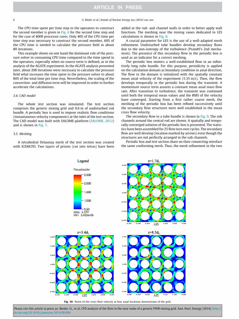
Fig. 10. Norm of the cross flow velocity at fou


added at the rod- and channel walls in order to better apply wallfunctions. The meshing near the mixing vanes dedicated to LEScalculations is shown in Fig. 8.

A crucial parameter for LES is the use of a well-adapted meshrefinement. Undisturbed tube bundles develop secondary flowsdue to the non-isotropy of the turbulence (Prandtl’s 2nd mecha-nism). The presence of this secondary flow in the periodic box isused as an indicator for a correct meshing.

The periodic box mimics a well-established flow in an infini-tively long tube bundle. For this purpose, periodicity is appliedon the calculation domain as boundary condition in axial direction.The flow in the domain is initialized with the spatially constantmean axial velocity of the experiment (5.35 m/s). Then, the flowdevelops temporally in the periodic box during the transient. Amomentum source term assures a constant mean axial mass flowrate. After transition to turbulence, the transient was continueduntil both the temporal mean values and the RMS of the velocityhave converged. Starting from a first rather coarse mesh, themeshing of the periodic box has been refined successively untilthe secondary flow structures were well established in the meancross flow velocity.

The secondary flow in a tube bundle is shown in Fig. 9. The subchannels around the central rod are shown. A spatially and tempo-rally converged solution of the periodic box is presented. The statis-tics have been assembled for 25 flow turn over cycles. The secondaryflow are well develop (location marked by arrows) even though thestructures are not perfectly arranged in the sub channels.

Periodic box and test section share on their connecting interfacethe same conforming mesh. Thus, the mesh refinement in the two

z=1

z=8

z=1.7d

z=8.5d

.7dh

.5dh

r axial locations downstream of the grid.




z=1.7dh d5.8=z hAGATE AGATE

LES LES

k-ε -k ε

Fig. 11. Comparison of the measured and calculated velocity.


parts is indicial and we have determined per se the meshing withthe smallest mesh number which is able to develop secondary flowstructures. The final mesh for LES calculations has about 300million velocity calculation points (degree of liberty >109). Decom-posing the calculation domain with METIS on 4600 processor cores


leads to about 32,600 tetrahedral cells or 38,500 pressure points,respectively, per partition. As shown before, a good parallel perfor-mance is assured for this partitioning.

For k–e calculations the mesh is significantly sparser than theLES mesh. Starting from a relatively sparse first mesh, meshing





independent results have been obtained after four successiverefinements. This final mesh has of about 30 million velocity calcu-lation points.

3.6. Calculation procedure

The LES calculation procedure consists of three successivesteps:

1. A transient of the periodic box is calculated standalone until themean velocity is converged. The mean axial velocity of theexperiment is imposed as initial condition and kept constantduring the transient.

2. Then the periodic box is connected to the AGATE test sectionand both periodic box and test section are simulated simulta-neously. At each time step, the result of the instantaneousvelocity of the periodic box is imposed at the test section inlet.The transient was continued until the fluctuations in the wholetest section were stabilized.

3. After stabilization of the flow, the statistics have been assem-bled in the whole test section during a transient in whom theflow has traversed twice the whole calculation domain.

As a consequence of this relatively short integration period, thestatistics (mean values and RMS) were converged only up to about25dh downstream of the grid.

The k–e modelling calculation procedure consists of two succes-sive steps:

1. A transient of the periodic box was calculated standalone untilvelocity, k and e are converged. The mean axial velocity of theexperiment is imposed as initial condition and kept constantduring the transient. The steady state solution of k and e is onlya function of the velocity and thus independent of their initialvalues.

2. Then the periodic box is connected to the AGATE test sectionand both periodic box and test section are simulated simulta-neously. At each time step, the steady state solution of thevelocity, k and e of the inlet box are imposed at the test sectioninlet. The transient was continued until velocity, k and e areconverged in the test section.

As the solution of the periodic box has converged, the additionalCPU time the code spends in the periodic box is negligible withrespect to the time spend in the test section.

Fig. 12. At z = 1.7dh; measured and calculated velocity profiles normal to the axis atx = 0.0063 and at y = 0.0063.

4. Results

The flow leaves the mixing grid and advances axially in the testsection. The related evolution of the norm of the mean cross flowvelocity (jv j ¼

ffiffiffiffiffiffiffiffiffiffiffiffiffiffiffiffiffiv2

x þ v2y

q) is shown qualitatively in Fig. 10 for the

LES calculation. Three distances from the mixing grid are selectedfor the visualization and z = 0 corresponds to the upper edge ofthe mixing grid (in the sense of the flow direction):

� At z = 1.7dh, the mixing vanes impose a very complex flow withtiny swirling structures.� At z = 3.4dh, the swirling structures are rearranged and start to

form the predominant 45� diagonal flow.� At z = 8.5dh, the flow is circling around the central rod by keep-

ing at the same time the 45� diagonal orientation.

The vectors of the mean cross flow velocity are shown in Fig. 11for z = 1.7dh and z = 8.5dh. The measured vectors are compared tothe vectors of the k–e and the LES calculation. In the gaps between


the rods only one component of the velocity vector is measurablewith LDV (vx along beam lines normal to the y-axis and vy alongbeam lines normal to the x-axis). Thus, the measured vector fieldcontains less information than the calculated ones. Nevertheless,the 45� diagonal structure of the flow is well visible in the mea-surement. For z = 8.5dh the measured vectors are scaled up forgraphical reasons by a factor 3.

Close to the grid at z = 1.7dh the LES calculation shows fourswirls in each sub channel which are partly located in the gapsbetween the rods. These are the main swirls imposed by the mix-ing vanes. The k–e calculation shows only two swirls in each subchannel which are also partly located in the gaps between the rods.The 45� diagonal flow structure is visible in both turbulence mod-elling approaches. Unfortunately, the swirls cannot be detected bythe LDA measurements, for they are partly located in areas whichare not accessible by the laser beam.

At z = 8.5dh the LES calculation shows a new arrangement of thecross flow which forms larger swirls turning in the sub channelsand around the central rod. The swirls in the sub channels disap-pear in the k–e calculation and a predominant diagonal flow at45� is established. A quantitative comparison of measured and cal-culated velocity profiles is given in Fig. 12 for z = 1.7dh and inFig. 13 for z = 8.5dh. Both turbulence modelling approaches (LESand k–e) are considered. At the top of Fig. 12 and Fig. 13 the axialvelocity vz and the cross flow velocity in y direction vy are shown




Fig. 13. At z = 8.5dh; measured and calculated velocity profiles normal to the axis atx = 0.0063 and at y = 0.0063.


along a line orthogonally to the x-axis at x = 0.0063 m which spanin y direction the whole cannel width. At the bottom of Fig. 12 andFig 13 the axial velocity vz and the cross flow velocity in x directionvx are shown along a line orthogonally to the y-axis at y = 0.0063 mwhich span in x direction the whole cannel width. The position ofboth profiles is added to Fig. 10.

Both turbulence modelling approaches reproduce correctly themeasured cross flow velocity profiles; the differences betweenmeasured and calculated cross flow velocities are marginal. Theaxial velocity vz however is overestimated by the k–e model fur-ther downstream of the grid. At the location z = 8.5dh, the LESclearly reproduces the measured axial velocity better than thek–e model. The reason of this overestimation is that the turbulentviscosity in the sub-channel centers is overestimated by the k–emodel. Thus, when searching for mesh convergence as requestedby best practice guidelines (Mahaffy et al., 2007), the k–e modelsystematically overestimates the maximum velocity in the centerof a sub-channel.

The here detected good agreement of the velocity distributionin the near wake of mixing grids between measurement, LES andlinear eddy viscosity modelling (k–e) confirms an analogous resultestablish in the MATHIS_H benchmark (Lee et al., 2012; Smithet al., 2013). The cross flow patterns in the near wake can be insen-sitive to the turbulence model due to the dominance of inertiaforces which are related to the geometry of the mixing vanes. Thus,turbulence models should not be validated in the near wake of


mixing grids by comparing cross flow velocity profiles. Neverthe-less, the good agreement between the profiles is more thansurprising when looking at Fig. 10, where the global flow behaviorcalculated by LES and k–e model is clearly different. Maybe, com-paring velocity profiles traversing the centers of the sub channelis not the best indicator for the quality of a calculation. Moredetailed experimental data, especially in zones not accessible byLDV measurements form the channel side are needed, as reportede.g., by Lascar et al. (2013).

5. Code performance

The LES calculation in the test section (initialization andtransient) has been performed on 4600 processor cores of theCURIE cluster of the TGCC (TGCC, 2013). 20 CPU days were neces-sary to initialize and to converge the mean values of the velocity inthe whole calculation domain; the RMS values of the velocity fluc-tuations were not fully converge at axial distances z > 25dh.

6. Conclusion

The flow in a rod assembly with mixing grid has been analyzedexperimentally and numerically. Numerically, two types of turbu-lence modelling approaches (LES and k–e) have been applied. Themeshing of the LES calculation contains 300 million controlvolumes for the velocity and the calculation has been performedwith the Trio_U code in parallel on 4600 processor cores. It hasbeen verified that Trio_U scales well on this kind of parallelcalculations.

For various distances from the mixing grid, calculated horizon-tal profiles of the cross flow velocity and of the axial velocity arecompared to measurements. The mean cross flow velocitycalculated by both LES and the k–e model match the experimentalvalues. At first glance, it seems that even linear turbulent viscositymodels can reproduce the mean cross flow velocity directly down-stream of the mixing grid. However, the flow patterns seem to beinsensitive to the turbulence model in this region due to the dom-inance of inertia forces which again are related to the geometry ofthe mixing vanes. Thus, the application of turbulence modelsshould not be tested close to mixing grids.

Acknowledgement

The authors are grateful to AREVA for giving the authorizationto use the experimental data.

References

Bieder U., 2012. Analysis of the flow down- and upwind of split type mixing vanes.In: Proceedings of the CFD4NRS_4 conference, 10–12 September 2012, Daejon,Korea.

Calvin, C., Cueto, O., Emonot, P., 2002. An object-oriented approach to the design offluid mechanics software. ESAIM: Mathematical Modelling and NumericalAnalysis – Modélisation Mathématique et Analyse Numérique. 36.5, 907-921.<http://eudml.org/doc/245828>.

Ducros, F., Bieder, U., Cioni, O., Fortin, T., Fournier, B., Fauchet, G., Quéméré, P., 2010.Verification and validation considerations regarding the qualification ofnumerical schemes for LES for dilution problems. Nucl. Eng. Des. 240, 2123–2130.

Falk, F., Mempontail, A., 1998. Détermination d’un champ de vitesses 3D engéométrie complexe par vélocimétrie laser 2 dimensions. 6ème congrèsfrancophone de vélocimétrie laser, Saint-Louis, 22–25 Septembre 1998.

Fortin T., 2006. Une méthode d’éléments finis à décomposition L2 d’ordre élevémotivée par la simulation des écoulements diphasiques bas Mach (PhD thesis),Université Paris VI.

Guermond, J.L., Quartapelle, L., 1998. On the stability and convergence of projectionmethods based on pressure poisson equation. Int. J. Numer. Methods Fluids 26,1039–1053.

Hirt, C.V., Nichols, B.D., Romero, N.C., 1975. SOLA – A numerical solution algorithmfor transient flow. Los Alamos National Lab., Report LA-5852.


http://www.eudml.org/doc/245828

http://refhub.elsevier.com/S0306-4549(14)00389-2/h0020










Kuzmin, D., Turek, S., 2004. High-resolution FEM-TVD schemes based on a fullymultidimensional flux limit. J. Comput. Phys. 198, 131–158.

Lascar, C., Marjolaine, P., Goodheart, K., Martin, M., Hatman, A., Simoneau, J.P., 2013.Validation of CFD Methodology to predict flow fields within rod bundles withspacer grids. In: 15th International Topical Meeting on Nuclear ReactorThermal-Hydraulics, NURETH-15, Pisa, Italy.

Lee, J.R., Kim, J., Song, C.H., 2012. Synthesis of the OCDE/NEA-KAERI Rod Bundle CFDBenchmark Exercise Proceedings of the CFD4NRS_4 conference, Daejon, Korea,10–12 September.

Mahaffy, J., et al., 2007. Best practice Guidelines for the Use of CFD in Nuclear SafetyApplications.NEA/CSNI/R(2007)5. <http://www.nea.fr/html/nsd/docs/2007/csni-r2007-5.pdf>.


METIS, 2013. <http://glaros.dtc.umn.edu/gkhome/metis/metis/overview>.PETSc, 2014. <http://www.mcs.anl.gov/petsc/>.SALOME, 2012. <http://www.salome-platform.org/>.Smith, B.L., Song, C.H., Chang, S.K., Lee, J.R., Amri, A., 2013. The OECD-KAERI CFD

benchmarking exercise based on flow mixing in a rod bundle. In: 15thInternational Topical Meeting on Nuclear Reactor Thermal Hydraulics,NURETH-15, Pisa, Italy.

TGCC, 2013. <http://www-hpc.cea.fr/fr/complexe/tgcc-curie.htm>.Trio_U, 2006. <http://www-trio-u.cea.fr/>.




http://www.nea.fr/html/nsd/docs/2007/csni-r2007-5.pdf

http://www.nea.fr/html/nsd/docs/2007/csni-r2007-5.pdf

http://www.glaros.dtc.umn.edu/gkhome/metis/metis/overview

http://www.mcs.anl.gov/petsc/

http://www.salome-platform.org/

http://www-hpc.cea.fr/fr/complexe/tgcc-curie.htm

http://www-trio-u.cea.fr/



Documents

CFD analysis of the flow in the near wake of a generic PWR mixing grid