CFD and Thermography Techniques Applied in Cooling Systems

7

CFD and Thermography Techniques Applied in Cooling Systems Designs

Samuel Santos Borges and Cassiano Antunes Cezario Research and Technological Innovation Department, WEG

Brazil

1. Introduction

The focus of this work consists in optimizing the water flow inside a water cooled electric motor frame, aiming at the maximization of the power/frame size ratio, the minimization of pressure drop and the avoidance of hot spots. For the development of this work computational fluid dynamics (CFD) and thermography techniques were used. For many years water cooled electric motors have been used by industry, especially in specific applications that require features that can not be provided by conventional fan cooled motors. Among theses features are a better power/frame size relation, low noise levels, enclose applications, among others. Cooling by means of water circulation is frequently used in large motors, typically frame sizes above IEC 315. A justification for this practice not to be widely used in smaller motors is its higher cost compared to air cooling systems. However, provided that it presents some technical and/or economical viability, water cooling can also be used in smaller frame sizes. The technological progress have resulted in the development of new tools that facilitate the study of this motor type, such as the computational fluid dynamics and the thermography techniques, which consist, respectively, in the use of numeric models applied to fluid mechanics and the obtaining of the motor surface temperature distribution.

2. Benefits and drawbacks

The following advantages and disadvantages of this kind of motor can be mentioned, in comparison with air cooled motors.

2.1 Advantages Greater power/frame size ratio;

Lower noise level;

Higher efficiency;

The outside waste deposit on the frame does not damage the motor cooling;

No problems with waste deposit on the external fan blade;

It can be used in totally enclosure environment;

The heat removed from the motor is not directly dissipated into the environment;

Possibility of using the same cooling fluid of the load and/or machine where it is installed;

www.intechopen.com

Applied Computational Fluid Dynamics

136

Better resistance to local impact.

2.2 Disadvantages Higher manufacturing cost;

Auxiliary system to provide water;

Need to control the water chemical composition;

Risk of corrosion inside of the water circuit;

Risk of fouling in the water circuit;

Risk of leaks;

More precautions on maintenance.

3. Fundamental concepts

3.1 Cooling system The cooling systems are apparatus usually comprised of several components that interact to keep the temperature of machines and systems in general controlled in order not to exceed the limits imposed by quality, safety, performance and/or efficiency. For instance, systems such as internal combustion engines, turbines, compressors, bearings, electric machines, electronic structures, electrical conductors, chemical and welding processes, among many others, can be mentioned as some examples of systems comprising thermal restrictions. Consequently, the cooling systems are very important to industries and should therefore be designed to keep a good performance and reliability. The more commonly used coolants are gases and liquids. Among them, due to their wide occurrence, low cost and practicality, air and water are customarily employed. They can be used in many different ways: in direct or indirect contact with the systems, by means of one or more fluid combinations, separated or mixed. And they can be forcedly or naturally moved, by physical mechanisms respectively known as forced convection and natural convection.

3.2 Heat transfer Heat transfer concerns the exchange of thermal energy from one region of higher temperature to another of lower temperature in one or more means. This exchange occurs by mechanisms as conduction, convection, radiation and phase-change.

3.2.1 Conduction The conduction occurs due to interactions between the particles of fluids. Thermal insulation, tanks, plates and ducts walls, fins, and others are examples of devices that exchange heat by conduction. It is described by Fourier’s Law and the following equation:

k

Tq kA

n

(1)

Where, qk: Heat flux of conduction; K: Thermal conductivity; A: Heat transfer area;

T : Temperature gradient;

n: Direction.

www.intechopen.com


137

3.2.2 Convection The convection is the heat transfer between a solid surface and a moving fluid. This

phenomenon can be natural, induced by density difference (low fluid velocity), or forced,

customarily supplied by fans or pumps (high fluid velocity).

( )h sq hA T T (2)

Where, qh: Heat flux of convection; h: Convection coefficient; A: Heat transfer area; Ts: Surface temperature; T∞: Fluid temperature.

3.2.3 Radiation The thermal radiation is provided by electromagnetic waves emission. The classic example

of this phenomenon is the heat transfer between sun and earth. It is given by Stefan-

Boltzmann Law.

4 4

1 2( )rq T T (3)

Where, qr: Heat flux of radiation; ε: Emissivity; σ: Stefan-Boltzmann constant; T1, T2: Surface temperatures.

3.2.4 Phase – Change It is boiling, condensation, freezing and melting. These processes are given by following

equations.

.Q m H (4)

Where, Q: Amount of heat; m: Mass; ΔH: Specific latent heat.

3.2.5 Heat transfer in conduits In the heat transfer in the fluid flowing in a conduit, the temperature is neither uniform in

the fluid flow direction nor in the heat flux direction. Therefore, the bulk temperature is

assumed as reference temperature. The use of a temperature reference allows to execute the

heat balance in steady state. In this case, the transferred heat per time unit is a direct

measure of the bulk temperature difference between two conduit sections. That is,

. .p bq m c T (5)

www.intechopen.com


138

Where, q: Amount of heat per time unit;

m : Mass flow rate;

cp: Specific heat of fluid; ΔTb: Bulk temperature difference of fluid among two conduit sections.

3.3 Fluid dynamics 3.3.1 Mass flow rate The mass flow rate is given by the mass of fluid which passes through a surface per time

unit and can be calculated from the following equation:

. .m v A (6)

Where,

m : Mass flow rate;

ρ: Fluid density; v: Mean velocity in the section; A: Area of conduit section.

3.3.2 Pressure drop The pressure drop in pipes may be occasioned by means of:

Localized drops (valves, curves, and others);

Friction;

Difference of piping height. The pressure drop is obtained as a function of Reynolds number, which depends on the

fluid velocity, given by:

. .

Rev D (7)

Where,

Re: Reynolds number; ρ: Fluid density; v: Mean velocity in the section; D: Diameter of pipe; μ: Viscosity. If the Reynolds number is smaller than 2300 the flow is laminar and friction factor is

calculated by:

64

Ref (8)

Where,

f: Friction factor; Re: Reynolds number. But, if the Reynolds number is greater than 2300 the flow is turbulent and friction factor is

calculated by:

www.intechopen.com


139

1 2.512.log

3.7 Re.

eD

f f

(9)

Where, f: Friction factor; Re: Reynolds number; e: Absolute roughness; D: Pipe diameter. And the pressure drop is determined by:

2.

. .2

L vp f

D

(10)

Where, Δp: Pressure drop; f: Friction factor; L: Length of pipe; D: Pipe diameter; ρ: Fluid density; v: Mean velocity in the section. Therefore, to minimize the pressure drop and consequently reduce the energy loss of flow, it is desired low fluid velocity.

3.4 Turbulence models Among several turbulence models known in the literature, will be discussed here only those ones involved in this work: κ - ε model, κ - ω model and Shear-Stress Transport (SST).

3.4.1 The κ - ε model The simplest complete turbulence model has a wide range of applications in industrial and engineering problems. It can be applied to mass or heat transfer, combustion, multi-phase flows simulations, and others. The κ - ε model has been incorporated in most commercial CFD codes due to its stability and numerical robustness, good accuracy and low computational cost. This model should be avoided in complex flow applications, such as flows with boundary layer separation, sudden changes in the mean strain rate, rotating fluids, and over curved surfaces. The standard κ - ε model is based on model transport equations for the turbulence kinetic energy κ and its dissipation rate ε. Transport equations for the standard κ - ε model are given by:

( ) ( )i t

k b M ki j k j

k k kP P Y S

t x x x

(11)

2

1 3 2

( ) ( ).

i tk b

i j j

C P C P C St x x x

(12)

www.intechopen.com


140

Where, μt: Turbulent viscosity; Pk: Generation of turbulence kinetic energy due to the mean velocity gradients; Pb: Generation of turbulence kinetic energy due to buoyancy; YM: Fluctuating dilatation in compressible turbulence; ρ: Density; μ: Viscosity; C1ε, C2ε, C3ε: Model constants;

σk, σε: Turbulent Prandtl number for κ and ε; Sk, Sε: Source term.

3.4.2 The κ - ω model The κ - ω model is widely used and is superior for boundary-layer flows both in the viscous

near-wall region treatment and in the streamwise pressure gradients application. However,

it is not appropriate outside the shear layer that is a free-stream boundary. The standard κ - ω model is an empirical model based on model transport equations for the turbulence

kinetic energy κ and the specific dissipation rate ω, which is obtained by ε to κ ratio. Based

on Wilcox, κ and ω are obtained from:

( )( )

'j t

k kbj j k j

U kk kP P

t x x x

(13)

2

( )( ) j tk b

j j j

UP P

t x x x

(14)

Pκb, Pωb: Turbulence buoyancy term; U: Velocity vector; σω: Turbulent Prandtl number for ω; ┚’, ┚, ┙: Model constant.

3.4.3 The shear-stress transport model (SST) The shear-stress transport κ - ω model was developed by Menter to effectively blend the robust

and accurate formulation of the κ - ω model in the near-wall region with the free-stream

independence of the κ - ε model in the far field. To achieve this, the κ - ε model is converted

into a κ - ω formulation. The SST κ - ω model is similar to the standard κ - ω model, but the

modeling constants are different in one and another and the SST model includes some changes

in the standard one, such as the multiplication of both transformed κ - ε and κ - ω models by a

blending function, which activates standard κ - ω model in the near-wall region and activates

transformed κ - ε model away from the surface, the incorporation of a damped cross-diffusion

derivative term in the ω equation, and a modification in the definition of the turbulent

viscosity to account for the transport of the turbulent shear stress.

These improvements provide more accuracy and reliability for a wide range of flow classes

than the standard κ - ω model. For instance, adverse pressure gradient flows, airfoils, and

transonic shock waves.

www.intechopen.com


141

The base equations are:

( ) ( )ik k k k

i j j

k k kG Y S

t x x x

(15)

( )( ) i

i j j

uG Y D S

t x x x

(16)

;tk

k

t (17)

Where,

kG : Generation of turbulence kinetic energy due to the mean velocity gradients; Gω: Generation of ω; Yk, Yω: Dissipation of κ and ω due to turbulence; Гk, Гω: Effective diffusivity of κ and ω; Gω: Cross-diffusion term; σω: Turbulent Prandtl number for ω; Sω: Source term.

3.4.4 Comparing SST and κ - ε model In the Figures 1 and 2 two simulations of temperature and velocity of the fluid are presented, with the same boundary conditions for SST and κ - ε model. Note that the results are similar for both models, however SST models capture more flow characteristics than κ - ε model.

Fig. 1. Fluid temperature using SST and κ - ε model

www.intechopen.com


142

Fig. 2. Fluid velocity using SST and κ - ε model

3.5 Fouling Fouling is a term employed to represent undesired accumulation of solid material on the

surfaces of heat exchangers. This accumulation results in thermal resistance increment

reducing exchanger performance. Fouling reduces the flow area and increases surface

roughness, causing a reduction in the flow rate as a consequence of the pressure drop

increase.

The fouling deposits may be loose particles or fix and hard layers, comprising sediments,

polymers, inorganic salts, fuel or corrosion products, biological growth, and others. The

maximum fouling layer can occur in few hours or may require many years to be formed. In

any case, it should be avoided, because it increases capital costs, maintenance costs,

production and energy losses, etc.

The main fouling mechanisms are crystallization, precipitation, sedimentation, chemical reaction, corrosion, biological and freezing fouling. The amount of heat per time unit can be calculated by:

. .q U A T (18)

Where, q: Amount of heat per time unit; U: Overall heat transfer coefficient; A: Heat transfer area; ΔT: Bulk temperature difference between two conduit sections. And U is obtained by the following equation:

www.intechopen.com


143

1

hec fou

UR R

(19)

Where, U: Overall heat transfer coefficient; Rhec: Resistance of cleaned heat exchanger; Rfou: Resistance of fouled heat exchanger. If the heat exchanger is clean, then Rfou = 0. Table 1 presents typical values of fouling resistance.

Table 1. Typical fouling resistance

Some variables must be taken into account in the design and operation of cooling systems,

in order to avoid fouling. The most important are:

Flow velocity: for water, it should be kept above 2 m/s to suppress fouling and above 1 m/s to minimize fouling. Surface temperature: for cooling towers, the water temperature must be kept below 60 °C. Tube material: select materials to avoid corrosion, for instance.

For liquid coolants, fouling inhibitors should be used, such as: corrosion inhibitors, anti-

dispersants, stabilizers, biocides, softeners, acids, and polyphosphates. However, if such

fouling controls are not effective, the exchanger must be cleaned either on-line or off-line.

3.6 Corrosion Corrosion is electrochemical destructive attack of the base material with its environment.

Water in direct contact with a metal surface causes oxidation, which is a process where

www.intechopen.com


144

metal dissolved in fluid; this phenomenon generates serious problems in the worldwide.

Corrosion causes:

Efficiency reduction of machines and plants;

Increase costs of maintenance and overdesign;

Losses or contaminations of products;

Plants shutdowns;

And others. The many aspects of corrosion problems constrain it control, which is achieved by recognizing and understanding corrosion mechanisms. The control and prevention of corrosion damage can be obtained basically by following methods:

Employment of suitable materials;

Use of protective coatings;

Change to the environment;

Application of cathodic or anodic protection and etc.

4. Water-cooled frame

The objective of this work consists in optimizing the water flow inside a water cooled frame considering the boundary conditions intrinsic to both the manufacturing process and the electric motor itself. One of the challenges of this development is the frame manufacturing, which consists in a single cast iron piece free of welds or seals, making it difficult to obtain the water circuit. Due to the increasing demand for smaller water cooled motors, in this work an IEC 200 frame size – 75 kW – IV Poles – 60 Hz motor was used.

5. Thermal circuit and equations

The first step of the design is the definition of the motor simplified thermal circuit as represented in Figure 3. It can be observed that the produced heat, L, is transferred through the equivalent resistance, Req, and the convection resistance, Rh, thus causing an increase in the average temperatures of the coil, Tw, the frame, Tframe and the fluid, Tfluid. The next step is calculating the water flow that is needed to remove the heat produced by the motor. This can be obtained by means of (20) and (5), where L is the heat amount to be

removed in W, m is the mass flow in kg/s, cp is the specific heat of water in J/(kg . K), To is

the outlet water temperature and Ti is the inlet water temperature both in K.

. .p o iL m c T T (20)

Using (20) and the values shown in Table 2, it is obtained a mass flow of 0.239 kg/s.

Variable Value

L 5.000 (W)

cp a 20 °C 4 184.3 (J / kg / K) To - Ti 5 (K)

Table 2. Value and units for variables

www.intechopen.com


145

Fig. 3. Simplified thermal circuit of the motor

The value of L was considered as the total losses of the motor, that is, it is considered that all

heat generated by the motor will be removed by water, which in practice does not happen,

once that a portion of generated heat will be dissipated to environment through the

endshields, the shaft and the terminal box. However, the heat portion removed by water is

greater than by other means, so that it can be considered conservative, thereby simplifying

the problem.

The next step consists in checking the circuit thermal saturation in relation to the water flow

that is, quantifying how much an increase in the flow causes the coil temperature to reduce.

Therefore, it is necessary to verify the behavior of the coil average temperature fluctuation,

ΔTw, with the water flow. For this verification equations obtained by heat transfer laws will

be used, as described next.

The equations (21) and (22) relate L in W with Tw, Tframe and Tfluid in K and with Req and Rh in K/W.

w frame

eq

T TL

R

(21)

frame fluid

h

T TL

R

(22)

And to obtain Rh it is used (23), where the convection coefficient, h, is in W / (m2 . K) and the thermal exchange surface between the frame and the fluid, A, is in m2.

1

.hR

h A (23)

www.intechopen.com


146

Fig. 4. Mass flow saturation

Knowing that h is a variable dependent on the fluid properties, the channel geometry and

the flow, then the fluctuation temperature, ΔTw, can be related to the mass flow m ,

according to (21), (22), (23), the fluid properties and the channel geometry, obtaining the curve presented in Figure 4. It can be observed that the motor operation point, Po, is located on the curve saturation region, what means that when increasing the water flow, the coil temperature reduction can be despised, because it is necessary a great increase the flow for the temperature to be slightly reduced. Therefore, this flow is correct for the design. For the obtainment of this curve the following considerations were made: a. Req is constant and, due to the difficulty to theoretically calculate its value, it was

obtained through (21) and (22) using experimental data of preliminary tests; b. Fluid properties are constant; c. Dimensions of channel: 0.400 x 0.015 m; d. Average diameter of the channel: 0,350 m.

6. Numerical analyses

Once analytically defined the flow value to be used in the design, the numerical analyses are initiated to check the water flow behavior inside the frame. For better use of the computational capacity, some considerations and simplifications were made concerning both the physical phenomenon and the geometry.

6.1 Heat transfer The possible hot spots inside the water circuit can be generated basically by three causes, local heat generation, cooling fluid shortage in determined regions, and/or fluid recirculation. For simulation purposes local heat generation is neglected, because the heat flow from the stator to the frame is uniformly distributed throughout the surface. As for fluid shortage, it can be considered that the water circuit will be totally filled and therefore

www.intechopen.com


147

there will be no shortage. So the possible hot spots will be generated only by water flow recirculation, thus allowing the elimination of the heat transfer calculation on the numerical simulations, making possible to identify the hot spots by means of association with the recirculation. It is emphasized that with this consideration the hot spots can be only identified, but not thermally quantified.

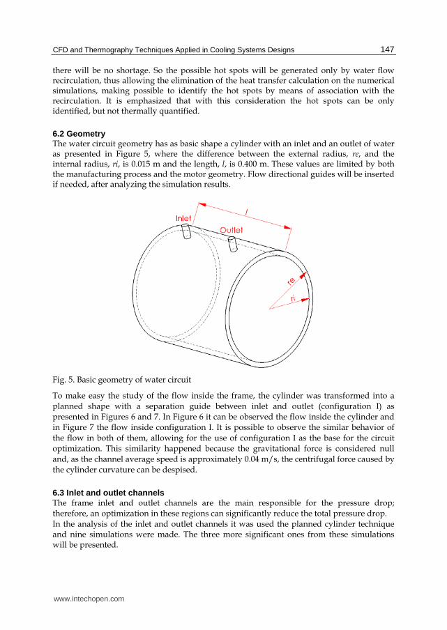
6.2 Geometry The water circuit geometry has as basic shape a cylinder with an inlet and an outlet of water as presented in Figure 5, where the difference between the external radius, re, and the internal radius, ri, is 0.015 m and the length, l, is 0.400 m. These values are limited by both the manufacturing process and the motor geometry. Flow directional guides will be inserted if needed, after analyzing the simulation results.

Fig. 5. Basic geometry of water circuit

To make easy the study of the flow inside the frame, the cylinder was transformed into a

planned shape with a separation guide between inlet and outlet (configuration I) as

presented in Figures 6 and 7. In Figure 6 it can be observed the flow inside the cylinder and

in Figure 7 the flow inside configuration I. It is possible to observe the similar behavior of

the flow in both of them, allowing for the use of configuration I as the base for the circuit

optimization. This similarity happened because the gravitational force is considered null

and, as the channel average speed is approximately 0.04 m/s, the centrifugal force caused by

the cylinder curvature can be despised.

6.3 Inlet and outlet channels The frame inlet and outlet channels are the main responsible for the pressure drop;

therefore, an optimization in these regions can significantly reduce the total pressure drop.

In the analysis of the inlet and outlet channels it was used the planned cylinder technique and nine simulations were made. The three more significant ones from these simulations will be presented.

www.intechopen.com


148

Fig. 6. Original cylinder

Fig. 7. Configuration I

The first simulation presented in Figure 8(a) consists in an inlet channel with circular pipe format located in the left side of the water main circuit. In this case, a water flow concentration is making tangent to the circuit walls occasioning a low flow in the middle of the circuit, which would cause an heterogeneous heat exchange. In the second case, presented in Figure 8(b), the flow was improved if compared with the first case. In this case a diffuser on the inlet, instead of a pipe, was used. The flow further improved when the inlet diffuser was moved to the middle of the main circuit that can be seen in the Figure 8(c).

www.intechopen.com


149

Fig. 8(a). Inlet and outlet channel

Fig. 8(b). Inlet and outlet channel

Fig. 8(c). Inlet and outlet channel

www.intechopen.com


150

Due to the similarities observed during the work between the flow behavior in the inlet and in the outlet channels, the improvement of the inlet channel also could be applied to the outlet channel.

6.4 Water circuit When the source of heat generation is constant in a surface, the cooling system needs to keep a constant fluid speed, keeping the heat transfer coefficient also constant in order to avoid undesired speed variation. Then, according to (24), where Q is the volumetric flow in m3/s, V the average speed in m/s and S the area of the transversal section of the flow in m2, in order to keep the speed constant, the ratio Q / S must be kept constant. In this case, as the flow is constant the area can also be kept constant throughout the circuit. Thus the whole design of the cooling circuit will be based on this premise.

.Q V S (24)

In accordance with the Figure 7 the configuration I presented a good flow, but without guides inside the circuit. The absence of these guides could compromise the frame stiffness; therefore, other configurations with guides inside the circuit were simulated. Among the 16 simulated configurations, it was initially expected that the configuration II would present a good result, what did not happen, because such configuration caused low speeds in the back of the guides, as shown in Figure 9. Due to the result obtained with the configuration II, the configuration III, presented in Figure 10, is proposed. In this configuration it was obtained the double water speed of the initial configuration I, besides presenting a good flow and low pressure drop.

Fig. 9. Configuration II – intercalated opposite guides

Fig. 10. Configuration III – central guide with curved guide

www.intechopen.com


151

6.5 Simulation data The simulation meshes were made with the software ICEM CFD 11.0.1. The used elements were prisms on the walls and tetras inside the mesh, always respecting the quality criterion Smooth Elements Globally – Quality with value above 0.2. The simulations were made with the software CFX 11.0, using the following simulation parameters:

Heat transfer: None;

Buoyance: Non buoyancy;

Turbulence: Shear Stress Transport;

Convergence criteria: 10-5 (RMS).

7. Experiments and thermography

As yet only one motor with water circuit similar to the configuration I was tested. Due to the manufacturing process the dividing guide had been interrupted, therefore, the water inlet and outlet were not separated. This fact was confirmed using thermography techniques.

7.1 Thermal visualization techniques To check the guide arrangement inside the channel the following procedure was accomplished: the motor was turned on and kept running for 30 minutes without water circulation. The water inlet valve was then opened, while keeping the motor working. The phenomenon of water filling in the frame channel was recorded by the thermographic camera. The sequence captured on the video can be visualized in Figure 11. In this case, the outlet is located on the top and not on the lateral of the frame, thus assuring the removal of air from the frame inside, as presented in Figures 11(d) and 11(e).

Fig. 11(a). Water filling frame channel - Closed valve

www.intechopen.com


152

Fig. 11(b). Water filling frame channel - time: 10 s

Fig. 11(c). Water filling frame channel - time: 1 min and 10 s

Fig. 11(d). Water filling frame channel - time: 3 min and 10 s

www.intechopen.com


153

Fig. 11(e). Water filling frame channel - time: 10 min

Through this test it can be observed that two dark bands appear between the inlet and the outlet, allowing to affirm that two openings exist on the dividing guide. Theses bands can be

visualized in Figures. 11(d) and 11(e). Therefore, when the outlet is located on the frame lateral, as proposed in the configuration I, the flow passes directly from the inlet to the outlet.

7.2 Results Although the dividing guide between inlet and outlet to have been interrupted, thus causing recirculation, this motor presented a temperature rise of 73 °C on the windings,

below the higher limit of its thermal class (80 °C).

7.3 Final considerations The next steps of this work consist in testing motors of higher power rates in the same frame size using the configuration III previously presented. When increasing the power in these frames, the bearing temperature can be a limiting factor for the motor integrity. Therefore, it is also intended to design motors with water cooled bearings. Note that in this design step the fouling and corrosion were not considered, however, due to its meaning should be contemplated before product execution.

8. Conclusions

With the support of the CFD technique it was possible to foresee the water flow behavior inside the frame channel without visualizing directly the water flow. Through the use of the CFD it was also possible to double the water speed inside the frame channel, thus reducing the pressure drop in 18 % when compared with the initial design. Another advantages provided by CFD were the reduction obtained both in the development time and in the number of prototypes. These advantages have been proven in this work: in spite of the 22 frame configurations that have been initially proposed, after the simulation results were obtained only the three best prototypes have been actually manufactured. The use of thermography techniques in the field of electric motors helps to improve not only the development of products, but also the quality control and the maintenance of operating

www.intechopen.com


154

machines in the field. In this case, specifically, it was possible to visualize the guides configuration and the water flow inside the frame channel preventing the need to destroy it.

9. Acknowledgement

The authors would like to thank all Weg colleagues that directly or indirectly participated in this project.

10. References

Fox, R. W. & Mcdonald, A. T., Introdução à mecânica dos Fluidos, fifth edition, 2001. Incropera, F. P. & Witt, D. P., Introduction to Heat transfer, second edition by John Wiley &

Sons, 1985. John H. Lienhard IV & V, A Heat Transfer Textbook, third edition, published by Phlogiston

Press, 2004. Jones, W. P. & Launder, B. E. (1972), The Prediction of Laminarization with a Two-Equation

Model of Turbulence, International Journal of Heat and Mass Transfer, vol. 15, 1972, pp. 301-314.

Kreith, F., Princípio da transmissão de Calor, translation of the 3rd american edition, 1977. Kreith, F., The CRC Handbook of Thermal Engineering, CRC Press LLC, 2000. Launder, B. E. & Sharma, B. I. (1974), Application of the Energy Dissipation Model of Turbulence

to the Calculation of Flow Near a Spinning Disc, Letters in Heat and Mass Transfer, vol. 1, no. 2, pp. 131-138.

Launder, B. E. & Spalding, D. D., Mathematical Models of Turbulence, Academic Press, London, 1972.

Menter, F. R. (1993), Zonal Two Equation k-ω Turbulence Models for Aerodynamic Flows, AIAA Paper 93-2906.

Menter, F. R. (1994), Two-Equation Eddy-Viscosity Turbulence Models for Engineering Applications, AIAA Journal, vol. 32, no 8. pp. 1598-1605.

Nailen, R. L., Understanding the TEWAC Motor, IEEE Transactions on Industry Applications, vol. IA-11, nº. 4, July / august, 1975.

Roberge, P. R., Handbook of Corrosion Engineering, McGraw-Hill, 2000. Wilcox, D.C., Multiscale model for turbulent flows, In AIAA 24th Aerospace Sciences Meeting.

American Institute of Aeronautics and Astronautics, 1986.

www.intechopen.com

Applied Computational Fluid DynamicsEdited by Prof. Hyoung Woo Oh

ISBN 978-953-51-0271-7Hard cover, 344 pagesPublisher InTechPublished online 14, March, 2012Published in print edition March, 2012

InTech EuropeUniversity Campus STeP Ri Slavka Krautzeka 83/A 51000 Rijeka, Croatia Phone: +385 (51) 770 447 Fax: +385 (51) 686 166www.intechopen.com

InTech ChinaUnit 405, Office Block, Hotel Equatorial Shanghai No.65, Yan An Road (West), Shanghai, 200040, China

Phone: +86-21-62489820 Fax: +86-21-62489821

This book is served as a reference text to meet the needs of advanced scientists and research engineers whoseek for their own computational fluid dynamics (CFD) skills to solve a variety of fluid flow problems. KeyFeatures: - Flow Modeling in Sedimentation Tank, - Greenhouse Environment, - Hypersonic Aerodynamics, -Cooling Systems Design, - Photochemical Reaction Engineering, - Atmospheric Reentry Problem, - Fluid-Structure Interaction (FSI), - Atomization, - Hydraulic Component Design, - Air Conditioning System, -Industrial Applications of CFD

How to referenceIn order to correctly reference this scholarly work, feel free to copy and paste the following:

Samuel Santos Borges and Cassiano Antunes Cezario (2012). CFD and Thermography Techniques Applied inCooling Systems Designs, Applied Computational Fluid Dynamics, Prof. Hyoung Woo Oh (Ed.), ISBN: 978-953-51-0271-7, InTech, Available from: http://www.intechopen.com/books/applied-computational-fluid-dynamics/cfd-and-thermography-techniques-applied-in-cooling-systems-designs

© 2012 The Author(s). Licensee IntechOpen. This is an open access articledistributed under the terms of the Creative Commons Attribution 3.0License, which permits unrestricted use, distribution, and reproduction inany medium, provided the original work is properly cited.

http://creativecommons.org/licenses/by/3.0

Documents

CFD and Thermography Techniques Applied in Cooling Systems