Embed Size (px)
Citation preview

7/28/2019 CFD Modeling of Gas-Liquid-Solid Fluidized Bed
http://slidepdf.com/reader/full/cfd-modeling-of-gas-liquid-solid-fluidized-bed 1/57
i
Project Report on
CFD Modeling of Gas-Liquid-Solid Fluidized Bed
In partial fulfillment of the requirements of
Bachelor of Technology (Chemical Engineering)
Submitted By
Amit Kumar (Roll No.10500026)
Session: 2008-09
Under the guidance of
Mr. H.M. Jena
Department of Chemical Engineering
National Institute of Technology
Rourkela-769008
Orissa

7/28/2019 CFD Modeling of Gas-Liquid-Solid Fluidized Bed
http://slidepdf.com/reader/full/cfd-modeling-of-gas-liquid-solid-fluidized-bed 2/57
ii
CERTIFICATE
This is to certify that that the work in this thesis report entitled ― CFD Modeling of Gas-
Liquid-Solid Fluidized Bed‖ submitted by Amit Kumar in partial fulfillment of the
requirements for the degree of Bachelor of Technology in Chemical Engineering Session 2005-
2009 in the department of Chemical Engineering, National Institute of Technology Rourkela,
Rourkela is an authentic work carried out by him under my supervision and guidance.
To the best of my knowledge the matter embodied in the thesis has not been submitted to
any other University /Institute for the award of any degree.
Date: Mr. H. M. Jena
Department of Chemical Engineering
National Institute of Technology
Rourkela - 769008

7/28/2019 CFD Modeling of Gas-Liquid-Solid Fluidized Bed
http://slidepdf.com/reader/full/cfd-modeling-of-gas-liquid-solid-fluidized-bed 3/57
iii
ACKNOWLEDGEMENT
With a feeling of great pleasure, I express my sincere gratitude to Mr. H.M. Jena for his
superb guidance, support and constructive criticism, which led to the improvements and
completion of this project work .
I am thankful to Prof. R.K Singh and Prof. S.K. Maity for acting as project coordinator.
I am also grateful to Prof. K C Biswal, Head of the Department, Chemical Engineering for
providing the necessary opportunities for the completion of this project.
Amit Kumar (Roll No.10500026)
4th year
B. Tech.
Department of Chemical Engineering
National Institute of Technology, Rourkela

7/28/2019 CFD Modeling of Gas-Liquid-Solid Fluidized Bed
http://slidepdf.com/reader/full/cfd-modeling-of-gas-liquid-solid-fluidized-bed 4/57
iv
ABSTRACT
Gas – liquid – solid fluidized beds are used extensively in the refining, petrochemical,
pharmaceutical, biotechnology, food and environmental industries. Some of these processes usesolids whose densities are only slightly higher than the density of water. Because of the good
heat and mass transfer characteristics, three-phase fluidized beds or slurry bubble columns have
gained considerable importance in their application in physical, chemical, petrochemical,
electrochemical and biochemical processing.
This project report can be divided mainly into four parts. The first part discusses about
importance of gas-liquid-solid fluidized bed, their modes of operation, important hydrodynamic
properties those have been studied either related to modelling or experimental analysis and
applications of gas-liquid-solid fluidized bed. The second part gives an overview of the
methodology used in CFD to solve problems relating mass, momentum and heat transfer. Also
comparative study of various CFD related software is given in this section. Third part contains
the details about problem description and approach used in FLEUNT to get the solution. Finally
results of simulation and comparison with experimental results are shown.
The experimental setup was a fluidized bed of height 1.88m and diameter 10cm. The gas
(air) and liquid (water) is injected at the base with different velocities while taking glass beads of
different diameters as solid bed. The variables to be investigated are pressure drop, gas holdup
and bed expansion. It is required to verify the solutions of simulation by comparing it with
experimental results and then rest of the prediction can be done instead of carrying out the
experiments. In this way it helps to save the experimental costs and prevents from risk of
wastage of resources.

7/28/2019 CFD Modeling of Gas-Liquid-Solid Fluidized Bed
http://slidepdf.com/reader/full/cfd-modeling-of-gas-liquid-solid-fluidized-bed 5/57
v
CONTENTS
COVER PAGE i
CERTIFICATE ii
ACKNOWLEDGEMENT iii
ABSTRACT iv
CONTENTS v
LIST OF TABLES AND FIGURES vii
NOMENCLATURE ix
CHAPTER 1 LITERATURE REVIEW 1
1.1 Introduction 1
1.2 Applications of Gas-liquid-solid fluidized bed 21.3 Modes of operation of Gas-liquid-solid fluidized bed and flow regimes 3
1.4 Important hydrodynamic parameters studied in gas-liquid-solid fluidization 6
1.5 Present work: 9
CHAPTER 2 11
2.1 CFD (Computational Fluid Dynamics) 11
2.1.1 Discretization Methods in CFD 11
2.1.1.1 Finite difference method (FDM) 11
2.1.1.2 Finite volume method (FVM) 11
2.1.1.3 Finite element method (FEM) 12
2.1.2 How does a CFD code work? 12
2.1.2.1 Pre-Processing 13
2.1.2.2 Solver 14
2.1.2.3 Post-Processing 17
2.1.3 Advantages of CFD 17
2.2 CFD modeling of multiphase systems: 18
2.2.1 Approaches for numerical calculations of multiphase flows 19
2.2.1.1 The Euler-Lagrange Approach: 19
2.2.1.2 The Euler-Euler Approach 19
2.2.1.2.1 The VOF Model: 20

7/28/2019 CFD Modeling of Gas-Liquid-Solid Fluidized Bed
http://slidepdf.com/reader/full/cfd-modeling-of-gas-liquid-solid-fluidized-bed 6/57
vi
2.2.1.2.2 The Mixture Model: 20
2.2.1.2.3 The Eulerian Model 20
2.2.2 Choosing a multiphase model 20
CHAPTER 3 CFD SIMULATION OF GAS-LIQUID-SOLID FLUIDIZED BED 22
3.1 Computational flow model 22
3.1.1 Equations 22
3.1.2 Turbulence modelling: 23
3.2 Problem description: 24
3.3 Simulation 25
3.3.1 Geometry and Mesh 25
3.3.2 Selection of models for simulation 26
3.3.3 Solution 27
CHAPTER 4 RESULTS AND DISCUSSION 28
4.1 Phase Dynamics 29
4.2 Bed Expansion 30
4.3 Gas Holdup 34
4.4. Pressure Drop 36
CHAPTER 5 CONCLUSION 44
REFERENCES 45
.

7/28/2019 CFD Modeling of Gas-Liquid-Solid Fluidized Bed
http://slidepdf.com/reader/full/cfd-modeling-of-gas-liquid-solid-fluidized-bed 7/57
vii
LIST OF TABLES AND FIGURES
Table no. Caption Page
no.
Table 1 Important hydrodynamic parameters studied by CFD modeling of solid-liquid-gas
fluidized bed.
8
Table 2 Properties of air, water and glass beads used in experiment 24
Table 3 Model constants used for simulation 26
Figure no. Figure 1 Taxonomy of Three-Phase Fluidized Beds 4
Figure 2 Modes of operation of gas-liquid-solid fluidized bed 4
Figure 3 Schematic representation of the Mode I-a fluidized bed reactor 6
Figure 4 Algorithm of numerical approach used by simulation softwares 16
Figure 5 Experimental setup of fluidized bed column used (Static bed heights=17.1cm,21.3cm)
24
Figure 6 Coarse mesh and fine mesh created in GAMBIT 25
Figure 7 Plot of residuals for k-epsilon solver method as the iterations proceeds. 27
Figure 8 Contours of volume fraction of glass beads at water velocity of 0.12m/s and air velocity of 0.0125m/s with respect of time for initial bed height 21.3cm.
28
Figure 9 Contours of volume fractions of solid, liquid and gas at water velocity of 0.12m/sand air velocity of 0.0125m/s for initial bed height 21.3cm. 29
Figure 10 Velocity vector of glass beads in the column (actual and magnified) 30
Figure 11 Velocity vector of water in the column (actual and magnified) 31
Figure 12 Velocity vector of air in the column (actual and magnified) 32
Figure 13 XY plot of velocity magnitude of water 33
Figure 14 XY plot of velocity magnitude of air 33
Figure 15 Contours of volume fraction of glass beads with increasing water velocity at inlet air
velocity 0.05m/s for initial bed height 17.1cm and glass beads of size 2.18mm
34
Figure 16 XY plot of volume fraction of glass beads 35
Figure 17 Bed expansion vs. water velocity for initial bed height 17.1 cm and particle size
2.18mm
36

7/28/2019 CFD Modeling of Gas-Liquid-Solid Fluidized Bed
http://slidepdf.com/reader/full/cfd-modeling-of-gas-liquid-solid-fluidized-bed 8/57
viii
Figure 18 Bed expansion vs. water Velocity for initial bed height 21.3 cm and particle size2.18mm
36
Figure 19 Comparison of experimental results and simulated results obtained at air velocity0.05m/s and initial bed height 17.1 cm
37
Figure 20 Contour of air volume fraction at water velocity of 0.12m/s and air velocity of
0.0125m/s for initial bed height 21.3cm
38
Figure 21 Gas holdup vs. water velocity for initial bed height 17.1 cm and particle size2.18mm
38
Figure 22 Gas holdup vs. water velocity for initial bed height 21.3 cm and particle size
2.18mm
39
Figure 23 Gas holdup vs. water velocity for initial bed height 17.1 cm and particle size2.18mm
39
Figure 24 Gas holdup vs. air velocity for initial bed height 21.3 cm and particle size 2.18mm 40
Figure 25 Comparison of experimental result of gas holdup with that of simulated resultobtained at air inlet velocities 0.025 m/s and 0.05m/s for initial bed height 21.3 cm
40
Figure 26 Contours of static gauge pressure (mixture phase) in the column obtained at water velocity of 0.12m/s and air velocity of 0.0125m/s.
41
Figure 27 Pressure Drop vs. water velocity for initial bed height 17.1 cm and particle size2.18mm
42
Figure 28 Pressure Drop vs. water velocity for initial bed height 21.3 cm and particle size 2.18mm
42
Figure 29 Pressure Drop vs. Air velocity for initial bed height 17.1 cm and particle size
2.18mm
43
Figure 30 Pressure Drop vs. Air velocity for initial bed height 21.3 cm and particle size2.18mm
43
Figure 31 Comparison between pressure drop from experiment and that from simulation at air
inlet velocity 0.025 m/s and 0.025 m/s for initial bed height 21.3 cm
44

7/28/2019 CFD Modeling of Gas-Liquid-Solid Fluidized Bed
http://slidepdf.com/reader/full/cfd-modeling-of-gas-liquid-solid-fluidized-bed 9/57
ix
Nomenclature
ρk = Density of phase k= g (gas), l (liquid), s (solid)
εk = Volume fraction of phase k= g (gas), l (liquid), s (solid)
= Velocity of phase k= g (gas), l (liquid), s (solid)
P= Pressure
μeff = Effective viscosity
Mi,l= interphase force term for liquid phase
Mi,g= interphase force term for gas phase
Mi,s= interphase force term for solid phase
K= Turbulent kinetic energy
ε= Dissipation rate of turbulent kinetic energy
t= Time
g= Acceleration due to gravity

7/28/2019 CFD Modeling of Gas-Liquid-Solid Fluidized Bed
http://slidepdf.com/reader/full/cfd-modeling-of-gas-liquid-solid-fluidized-bed 10/57
1
CHAPTER 1
LITERATURE REVIEW1.1. INTRODUCTION
In a typical gas – liquid – solid three-phase fluidized bed, solid particles are fluidized primarily by upward concurrent flow of liquid and gas, with liquid as the continuous phase and
gas as dispersed bubbles if the superficial gas velocity is low. Because of the good heat and mass
transfer characteristics, three-phase fluidized beds or slurry bubble columns (ut < 0.05 m/s) have
gained considerable importance in their application in physical, chemical, petrochemical,
electrochemical and biochemical processing (L. S. Fan, 1989).
Gas – liquid – solid fluidized beds are used extensively in the refining, petrochemical,
pharmaceutical, biotechnology, food and environmental industries. Some of these processes use
solids whose densities are only slightly higher than the density of water (Bigot et al., 1990; Fan,
1989; Merchant; Nore, 1992).
Gas – liquid – solid fluidized beds can be operated with different hydrodynamic regimes,
which depend on the gas and liquid velocities, as well as the gas, liquid and solid properties. For
proper reactor modelling, it is essential to know under which regime the reactor will be operating
(Briens et al., 2005).
Two important hydrodynamic transitions within gas – liquid – solid fluidized beds are the
minimum liquid fluidization velocity, U Lmf , and the transition velocity from the coalesced to
dispersed bubble regime, U cd. The minimum liquid fluidization velocity is the superficial liquid
velocity at which the bed becomes fluidized for a given superficial gas velocity; above the
minimum liquid fluidization velocity, there is good contact between the gas, liquid and solid
phases which is essential for heat and mass transfer processes. In the coalesced bubble regime,
bubble size varies as the bubbles continuously coalesce and split, while in the dispersed bubble
regime, there is no coalescence and thus the bubble size is more uniform and generally smaller
(Luo et al., 1997).
Intensive investigations have been performed on three-phase fluidization over the past few
decades; however, there is still a lack of detailed physical understanding and predictive tools for
proper design, scale-up and optimum operation of such reactors. The calculation of
hydrodynamic parameters in these systems mainly relies on empirical correlations or semi-

7/28/2019 CFD Modeling of Gas-Liquid-Solid Fluidized Bed
http://slidepdf.com/reader/full/cfd-modeling-of-gas-liquid-solid-fluidized-bed 11/57
2
theoretical models such as the generalized wake model (Epstein et al., 1974) and the structured
wake model (L. S. Fan, 1989).
Though these models are capable of successfully elucidating the phenomena occurring in
the three-phase reactors, too many parameters in them have limited their practical applications.
In recent years, the computational fluid dynamics (CFD) based on the fundamental conservation
equations has become a viable technique for process simulation. Although powerful computer
capability is available today, CFD is very expensive in terms of computer resources and time for
full-scale, high-resolution, two- or three-dimensional simulation, and it is not readily applicable
for routine design and scale-up of industrial-scale units, at least at present. Hence, there is a
practical need to develop general and simple models for the three-phase fluidized beds. FLUENT
and CFX are tools normally used to get CFD solutions of three phase fluidized bed.
1.2. Applications of Gas-liquid-solid fluidized bed
Gas-liquid-solid fluidized beds have emerged in recent years as one of the most promising
devices for three-phase operations. Such devices are of considerable industrial importance as
evidenced by their wide use for chemical, petrochemical and biochemical processing. As three-
phase reactors, they have been employed in hydrogenation and hydrosulferization of residual oil
for coal liquefaction, in turbulent contacting absorption for flue gas desulphurization, and in the
bio-oxidation process for wastewater treatment. Three-phase fluidized beds are also often used in
physical operations.
The application of gas-liquid-solid fluidized bed systems to biotechnological processes
such as fermentation and aerobic wastewater treatment has gained considerable attention in
recent years. In these three-phase biotechnological processes, biologically catalytic agents, either
enzymes or living cells, are incorporated into the solid phase through immobilization techniques.
Typically, enzymes or living cells are entrapped within natural or synthetic polymer gel particles
or are attached to the surface of solid particles. Three-phase fluidized beds enjoy widespread use
in a number of applications including hydro treating and conversion of heavy petroleum and
synthetic crude, coal liquefaction, methanol production, conversion of glucose to ethanol and
various hydrogenation and oxidation reaction.
Fluidized bed units are also found in many plant operations in pharmaceuticals and mineral
industries. Fluidized beds serve many purposes in industry, such as facilitating catalytic and non-

7/28/2019 CFD Modeling of Gas-Liquid-Solid Fluidized Bed
http://slidepdf.com/reader/full/cfd-modeling-of-gas-liquid-solid-fluidized-bed 12/57
3
catalytic reactions, drying and other forms of mass transfer. They are especially useful in the fuel
and petroleum industry for things such as hydrocarbon cracking and reforming as well as
oxidation of naphthalene to phathalic anhydride (catalytic), or coking of petroleum residues
(non-catalytic). Catalytic reactions are carried out in fluidized beds by using a catalyst as the
cake in the column, and then introducing the reactants. In catalytic reactions, gas or liquid is
passed through a dry catalyst to speed up the reaction.
1.3. Modes of operation of Gas-liquid-solid fluidized bed and flow regimes
Gas-liquid-solid fluidization can be classified mainly into four modes of operation. These
modes are co-current three-phase fluidization with liquid as the continuous phase (mode I-a); co-
current three-phase fluidization with gas as the continuous phase (mode-I-b); inverse three-phase
fluidization (mode II-a); and fluidization represented by a turbulent contact absorber (TCA)
(mode II-b). Modes II-a and II-b are achieved with a countercurrent flow of gas and liquid. Due
to the complex nature of three-phase fluidization, however, various method are possible in
evaluating the operating and design parameters for each mode of operation.
Based on the differences in flow directions of gas and liquid and in contacting patterns
between the particles and the surrounding gas and liquid, several types of operation for gas-
liquid-solid fluidizations are possible. Three-phase fluidization is divided into two types
according to the relative direction of the gas and liquid flows, namely, co-current three-phase
fluidization and co-current three-phase fluidization (Bhatia and Epstein, 1974b; Epstein, 1981).
This is shown in Fig. 1.

7/28/2019 CFD Modeling of Gas-Liquid-Solid Fluidized Bed
http://slidepdf.com/reader/full/cfd-modeling-of-gas-liquid-solid-fluidized-bed 13/57
4
Fig.1. Taxonomy of Three-Phase Fluidized Beds (Epstein, 1981)
Fig.2. Modes of operation of gas-liquid-solid fluidized bed
7/28/2019 CFD Modeling of Gas-Liquid-Solid Fluidized Bed
http://slidepdf.com/reader/full/cfd-modeling-of-gas-liquid-solid-fluidized-bed 14/57
5
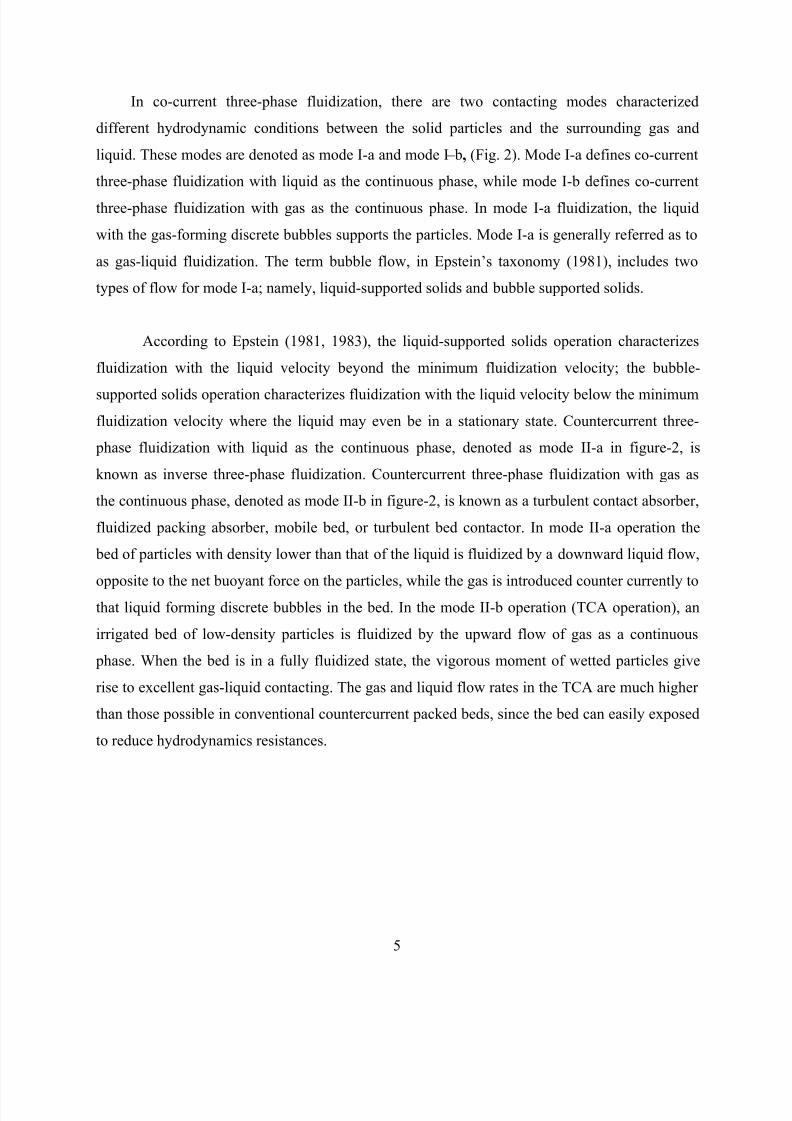
In co-current three-phase fluidization, there are two contacting modes characterized
different hydrodynamic conditions between the solid particles and the surrounding gas and
liquid. These modes are denoted as mode I-a and mode I – b, (Fig. 2). Mode I-a defines co-current
three-phase fluidization with liquid as the continuous phase, while mode I-b defines co-current
three-phase fluidization with gas as the continuous phase. In mode I-a fluidization, the liquid
with the gas-forming discrete bubbles supports the particles. Mode I-a is generally referred as to
as gas-liquid fluidization. The term bubble flow, in Epstein‘s taxonomy (1981), includes two
types of flow for mode I-a; namely, liquid-supported solids and bubble supported solids.
According to Epstein (1981, 1983), the liquid-supported solids operation characterizes
fluidization with the liquid velocity beyond the minimum fluidization velocity; the bubble-
supported solids operation characterizes fluidization with the liquid velocity below the minimum
fluidization velocity where the liquid may even be in a stationary state. Countercurrent three-
phase fluidization with liquid as the continuous phase, denoted as mode II-a in figure-2, is
known as inverse three-phase fluidization. Countercurrent three-phase fluidization with gas as
the continuous phase, denoted as mode II-b in figure-2, is known as a turbulent contact absorber,
fluidized packing absorber, mobile bed, or turbulent bed contactor. In mode II-a operation the
bed of particles with density lower than that of the liquid is fluidized by a downward liquid flow,
opposite to the net buoyant force on the particles, while the gas is introduced counter currently to
that liquid forming discrete bubbles in the bed. In the mode II-b operation (TCA operation), an
irrigated bed of low-density particles is fluidized by the upward flow of gas as a continuous
phase. When the bed is in a fully fluidized state, the vigorous moment of wetted particles give
rise to excellent gas-liquid contacting. The gas and liquid flow rates in the TCA are much higher
than those possible in conventional countercurrent packed beds, since the bed can easily exposed
to reduce hydrodynamics resistances.

7/28/2019 CFD Modeling of Gas-Liquid-Solid Fluidized Bed
http://slidepdf.com/reader/full/cfd-modeling-of-gas-liquid-solid-fluidized-bed 15/57
6
Fig.3. Schematic representation of the Mode I-a fluidized bed reactor
1.4. Important hydrodynamic parameters studied in gas-liquid-solid fluidization
Most of the previous studies related to three-phase fluidized bed reactors have been
directed towards the understanding the complex hydrodynamics, and its influence on the phase
holdup and transport properties. In literature, the hydrodynamic behavior, viz., the pressure drop,
minimum fluidization velocity, bed expansion and phase hold-up of a co-current gas – liquid –
solid three-phase fluidized bed, were examined using liquid as the continuous phase and gas as
the discontinuous phase (Jena et al. 2008). Recent research on fluidized bed reactors focuses on
the following topics:
7/28/2019 CFD Modeling of Gas-Liquid-Solid Fluidized Bed
http://slidepdf.com/reader/full/cfd-modeling-of-gas-liquid-solid-fluidized-bed 16/57
7
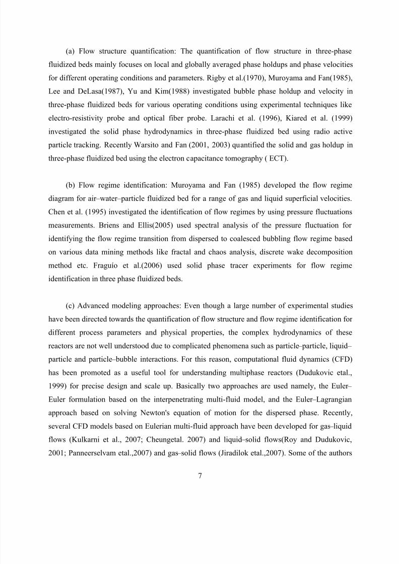
(a) Flow structure quantification: The quantification of flow structure in three-phase
fluidized beds mainly focuses on local and globally averaged phase holdups and phase velocities
for different operating conditions and parameters. Rigby et al.(1970), Muroyama and Fan(1985),
Lee and DeLasa(1987), Yu and Kim(1988) investigated bubble phase holdup and velocity in
three-phase fluidized beds for various operating conditions using experimental techniques like
electro-resistivity probe and optical fiber probe. Larachi et al. (1996), Kiared et al. (1999)
investigated the solid phase hydrodynamics in three-phase fluidized bed using radio active
particle tracking. Recently Warsito and Fan (2001, 2003) quantified the solid and gas holdup in
three-phase fluidized bed using the electron capacitance tomography ( ECT).
(b) Flow regime identification: Muroyama and Fan (1985) developed the flow regime
diagram for air – water – particle fluidized bed for a range of gas and liquid superficial velocities.
Chen et al. (1995) investigated the identification of flow regimes by using pressure fluctuations
measurements. Briens and Ellis(2005) used spectral analysis of the pressure fluctuation for
identifying the flow regime transition from dispersed to coalesced bubbling flow regime based
on various data mining methods like fractal and chaos analysis, discrete wake decomposition
method etc. Fraguío et al.(2006) used solid phase tracer experiments for flow regime
identification in three phase fluidized beds.
(c) Advanced modeling approaches: Even though a large number of experimental studies
have been directed towards the quantification of flow structure and flow regime identification for
different process parameters and physical properties, the complex hydrodynamics of these
reactors are not well understood due to complicated phenomena such as particle – particle, liquid –
particle and particle – bubble interactions. For this reason, computational fluid dynamics (CFD)
has been promoted as a useful tool for understanding multiphase reactors (Dudukovic etal.,
1999) for precise design and scale up. Basically two approaches are used namely, the Euler –
Euler formulation based on the interpenetrating multi-fluid model, and the Euler – Lagrangian
approach based on solving Newton's equation of motion for the dispersed phase. Recently,
several CFD models based on Eulerian multi-fluid approach have been developed for gas – liquid
flows (Kulkarni et al., 2007; Cheungetal. 2007) and liquid – solid flows(Roy and Dudukovic,
2001; Panneerselvam etal.,2007) and gas – solid flows (Jiradilok etal.,2007). Some of the authors

7/28/2019 CFD Modeling of Gas-Liquid-Solid Fluidized Bed
http://slidepdf.com/reader/full/cfd-modeling-of-gas-liquid-solid-fluidized-bed 17/57
8
(Matonis et al., 2002; Feng et al., 2005; Schallenberg et al.,2005) have extended these models to
three-phase flow systems.
Comprehensive list of literature on modeling of these reactors are tabulated in Table 1.
Most of these CFD studies are based on steady state, 2-D axis-symmetric, Eulerian multi-fluid
approach. But in general, three phase flows in fluidized bed reactors are intrinsically unsteady
and are composed of several flow processes occurring at different time and length scales. The
unsteady fluid dynamics often govern the mixing and transport processes and is inter-related in a
complex way with the design and operating parameters like reactor and sparger configuration,
gas flow rate and solid loading.
Table1. Important hydrodynamic parameters studied by CFD modeling of solid-liquid-gasfluidized bed.
Authors Multiphase approach Models used Parameter studied
Bahary et al. (1994) Multi fluid Eulerian
approach for three
phase fluidized bed
Gas phase was treated as a particulate
phase having 4mm diameter and a
kinetic theory granular flow model
applied for solid phase. They have
simulated both sym metric and axis-
symmetric mode
Verified the different flow
regimes in the fluidized
bed and compared the time
averaged axial solid
velocity with experimental
data
Grevskott et al.
(1996)
Two fluid Eulerian –
Eulerian model for
three phase bubble
column
The liquid phase along with the
particles is considered pseudo
homogeneous by modifying the
viscosity and density. They includedthe bubble size distribution based on
the bubble induced turbulent length
scale and the local turbulent kinetic
energy level
Studied the variation of
bubble size distribution,
liquid circulation and solid
movement
Mitra-Majumdar et
al.(1997)
2-D axis-symmetric,
multi-fluid Eulerian
approach for three-
phase bubble column
Used modified drag correlation
between the liquid and the gas phase
to account for the effect of solid
particles and between the solid of gas
bubbles. A k – ε turbulence model was
used for the turbulence and considered
the effect of bubbles on liquid phase
turbulence
Examined axial variation
of gas holdup and solid
hold up profiles for
various range of liquid and
gas superficial velocities
and solid circulation
velocity
Jianping and
Shonglin(1998)
2-D, Eulerian –
Eulerian method for
three-phase bubble
column
Pseudo-two-phase fluid dynamic
model. k sus− ε sus – k b− ε b turbulence
model used for turbulence
Validated local axial liquid
velocity and local gas
holdup with experimental
data
Padial et al. (2000) 3-D, multi-fluid
Eulerian approach for
three-phase draft- tube
bubble column
The drag force between solid particles
and gas bubbles was modeled in the
same way as that of drag force
between liquid and gas bubbles
Simulated gas volume
fraction and liquid
circulation in draft tube
bubble column. contd…
Matonis et
al.(2002)
3-D, multi-fluid
Eulerian approach for
Kinetic theory granular
flow(KTGF)model for describing the
Studied the time averaged
solid velocity and volume

7/28/2019 CFD Modeling of Gas-Liquid-Solid Fluidized Bed
http://slidepdf.com/reader/full/cfd-modeling-of-gas-liquid-solid-fluidized-bed 18/57
9
slurry bubble column particulate phase and a k – ε based
turbulence model for liquid phase
turbulence
fraction profiles, normal
and shear Reynolds stress
and comparison with
experimental data
Feng et al.(2005) 3-D, multi-fluid
Eulerian approach for
three-phase bubblecolumn
The liquid phase along with the solid
phase considered as a pseudo
homogeneous phase in view of theultrafine nanoparticles. The interface
force model of drag, lift and virtual
mass and k – ε model for turbulence
are included
Compared the local time
averaged liquid velocity
and gas holdup profilesalong the radial position
Schallenberg et
al.(2005)
3-D, multi-fluid
Eulerian approach for
three-phase bubble
column
Gas – liquid drag coefficient based on
single bubble rise, which is modified
for the effect of solid phase. Extended
k – ε turbulence model to account for
bubble-induced turbulence. The
interphase momentum between two
dispersed phases is included.
Validated local gas and
solid holdup as well as
liquid velocities with
experimental data
Li et al. (1999) 2-D, Eulerian –
Lagrangian model for
three-phase
fluidization
The Eulerian fluid dynamic (CFD)
method, the dispersed particle method
(DPM) and the volume-of-fluid (VOF)
method are used to account for the
flow of liquid, solid, and gas phases,
respectively. A continuum surface
force (CSF) model, a surface tension
force model and Newton's third law
are applied to account for the
interphase couplings of gas – liquid,
particle – bubble and particle – liquid
interactions, respectively. A close
distance interaction (CDI) model is
included in the particle – particle
collision analysis, which considers the
liquid interstitial effects betweencolliding particles
Investigated single bubble
rising velocity in a liquid –
solid fluidized bed and the
bubble wake structure and
bubble rise velocity in
liquid and liquid – solid
medium are simulated
Zhang and Ahmadi
(2005)
2-D, Eulerian –
Lagrangian model for
three-phase slurry
reactor
The interactions between bubble –
liquid and particle – liquid are included.
The drag, lift, buoyancy, and virtual
mass forces are also included.
Particle – particle and bubble – bubble
interactions are accounted for by the
hard sphere model approach. Bubble
coalescence is also included in the
model
Studied transient
characteristics of gas,
liquid, and particle phase
flows in terms of flow
structure and instantaneous
velocities. The effect of
bubble size on variation of
flow patterns are also
studied
1.5. Present work:
In the studies done so far, there has not been much emphasis on gas holdup and pressure
drop. Here, the focus is on understanding the complex hydrodynamics of three-phase fluidized
beds containing coarser particles of size above 1mm. The CFD software package FLUENT
6.2.16 has been used to simulate a solid-liquid-gas fluidized bed with a special designed air

7/28/2019 CFD Modeling of Gas-Liquid-Solid Fluidized Bed
http://slidepdf.com/reader/full/cfd-modeling-of-gas-liquid-solid-fluidized-bed 19/57
10
sparger aimed at improving the gas-liquid mixing in the distributor section and sending the well
mixed gas-liquid mixture to the fluidizing section. The fluidized bed to be simulated is of height
1.88m and diameter 0.1m. The gas (air) and liquid (water) has been injected at the base with
different velocities while taking glass beads of diameter 2.18mm as solid bed. The variables to
be investigated are bed expansion, gas holdup and pressure drop. The static bed heights of the
solid phase in the fluidized bed used for simulation are 17.1 cm and 21.3 cm. The simulated
results have been compared with the experimental results of Jena et al. (2008).
Definitions
Bed expansion: The height in the column up to which the solid phase is found in fluidized
condition.
Gas holdup: Gas holdup is defined as volume fraction of gas phase in that the column. In
contrast to gas-solid-liquid fluidized bed gas holdup is taken for expanded part of the column.Pressure drop: Pressure drop is defined as the difference of absolute pressure of inlet to
that of the outlet.

7/28/2019 CFD Modeling of Gas-Liquid-Solid Fluidized Bed
http://slidepdf.com/reader/full/cfd-modeling-of-gas-liquid-solid-fluidized-bed 20/57
11
CHAPTER 2
CFD IN MULTIPHASE MODELING
2.1. CFD (Computational Fluid Dynamics)
CFD is one of the branches of fluid mechanics that uses numerical methods and algorithmsto solve and analyze problems that involve fluid flows. Computers are used to perform the
millions of calculations required to simulate the interaction of fluids and gases with the complex
surfaces used in engineering. However, even with simplified equations and high speed
supercomputers, only approximate solutions can be achieved in many cases. More accurate codes
that can accurately and quickly simulate even complex scenarios such as supersonic or turbulent
flows are an ongoing area of research.
2.1.1. Discretization Methods in CFD
There are three discretization methods in CFD:
1. Finite difference method (FDM)
2. Finite volume method (FVM)
3. Finite element method (FEM)
2.1.1.1. Finite difference method (FDM): A finite difference method (FDM)
discretization is based upon the differential form of the PDE to be solved. Each derivative isreplaced with an approximate difference formula (that can generally be derived from a Taylor
series expansion). The computational domain is usually divided into hexahedral cells (the grid),
and the solution will be obtained at each nodal point. The FDM is easiest to understand when the
physical grid is Cartesian, but through the use of curvilinear transforms the method can be
extended to domains that are not easily represented by brick-shaped elements. The discretization
results in a system of equation of the variable at nodal points, and once a solution is found, then
we have a discrete representation of the solution.
2.1.1.2. Finite volume method (FVM): A finite volume method (FVM) discretization is
based upon an integral form of the PDE to be solved (e.g. conservation of mass, momentum, or
energy). The PDE is written in a form which can be solved for a given finite volume (or cell).
The computational domain is discretized into finite volumes and then for every volume the

7/28/2019 CFD Modeling of Gas-Liquid-Solid Fluidized Bed
http://slidepdf.com/reader/full/cfd-modeling-of-gas-liquid-solid-fluidized-bed 21/57
12
governing equations are solved. The resulting system of equations usually involves fluxes of the
conserved variable, and thus the calculation of fluxes is very important in FVM. The basic
advantage of this method over FDM is it does not require the use of structured grids, and the
effort to convert the given mesh in to structured numerical grid internally is completely avoided.
As with FDM, the resulting approximate solution is a discrete, but the variables are typically
placed at cell centers rather than at nodal points. This is not always true, as there are also face-
centered finite volume methods. In any case, the values of field variables at non-storage locations
(e.g. vertices) are obtained using interpolation.
2.1.1.3. Finite element method (FEM): A finite element method (FEM) discretization is
based upon a piecewise representation of the solution in terms of specified basis functions. The
computational domain is divided up into smaller domains (finite elements) and the solution in
each element is constructed from the basis functions. The actual equations that are solved are
typically obtained by restating the conservation equation in weak form: the field variables are
written in terms of the basis functions, the equation is multiplied by appropriate test functions,
and then integrated over an element. Since the FEM solution is in terms of specific basis
functions, a great deal more is known about the solution than for either FDM or FVM. This can
be a double-edged sword, as the choice of basis functions is very important and boundary
conditions may be more difficult to formulate. Again, a system of equations is obtained (usually
for nodal values) that must be solved to obtain a solution.
Comparison of the three methods is difficult, primarily due to the many variations of all
three methods. FVM and FDM provide discrete solutions, while FEM provides a continuous (up
to a point) solution. FVM and FDM are generally considered easier to program than FEM, but
opinions vary on this point. FVM are generally expected to provide better conservation
properties, but opinions vary on this point also.
2.1.2. How does a CFD code work?
CFD codes are structured around the numerical algorithms that can be tackle fluid
problems. In order to provide easy access to their solving power all commercial CFD packages
include sophisticated user interfaces input problem parameters and to examine the results. Hence
all codes contain three main elements:
7/28/2019 CFD Modeling of Gas-Liquid-Solid Fluidized Bed
http://slidepdf.com/reader/full/cfd-modeling-of-gas-liquid-solid-fluidized-bed 22/57
13
1. Pre-processing.
2. Solver
3. Post-processing.
2.1.2.1. Pre-Processing:
This is the first step in building and analyzing a flow model. Preprocessor consist of input
of a flow problem by means of an operator – friendly interface and subsequent transformation of
this input into form of suitable for the use by the solver. The user activities at the Pre-processing
stage involve:
• Definition of the geometry of the region: The computational domain.
• Grid generation the subdivision of the domain into a number of smaller, non-overlapping
sub domains (or control volumes or elements Selection of physical or chemical phenomena that
need to be modeled).
• Definition of fluid properties
• Specification of appropriate boundary conditions at cells, which coincide with or touch
the boundary. The solution of a flow problem (velocity, pressure, temperature etc.) is defined at
nodes inside each cell. The accuracy of CFD solutions is governed by number of cells in the grid.
In general, the larger numbers of cells better the solution accuracy. Both the accuracy of the
solution & its cost in terms of necessary computer hardware & calculation time are dependent on
the fineness of the grid. Efforts are underway to develop CFD codes with a (self) adaptive
meshing capability. Ultimately such programs will automatically refine the grid in areas of rapid
variation.
GAMBIT (CFD PREPROCESSOR): GAMBIT is a state-of-the-art preprocessor for
engineering analysis. With advanced geometry and meshing tools in a powerful, flexible, tightly-
integrated, and easy-to use interface, GAMBIT can dramatically reduce preprocessing times for
many applications. Complex models can be built directly within GAMBIT‘s solid geometry
modeler, or imported from any major CAD/CAE system. Using a virtual geometry overlay and
advanced cleanup tools, imported geometries are quickly converted into suitable flow domains.
A comprehensive set of highly-automated and size function driven meshing tools ensures that the
best mesh can be generated, whether structured, multiblock, unstructured, or hybrid.

7/28/2019 CFD Modeling of Gas-Liquid-Solid Fluidized Bed
http://slidepdf.com/reader/full/cfd-modeling-of-gas-liquid-solid-fluidized-bed 23/57
14
2.1.2.2. Solver:
The CFD solver does the flow calculations and produces the results. FLUENT,
FloWizard, FIDAP, CFX and POLYFLOW are some of the types of solvers. FLUENT is used in
most industries. FloWizard is the first general-purpose rapid flow modeling tool for design and
process engineers built by Fluent. POLYFLOW (and FIDAP) are also used in a wide range of
fields, with emphasis on the materials processing industries. FLUENT and CFX two solvers
were developed independently by ANSYS and have a number of things in common, but they also
have some significant differences. Both are control-volume based for high accuracy and rely
heavily on a pressure-based solution technique for broad applicability. They differ mainly in the
way they integrate the fluid flow equations and in their equation solution strategies. The CFX
solver uses finite elements (cell vertex numerics), similar to those used in mechanical analysis, to
discretize the domain. In contrast, the FLUENT solver uses finite volumes (cell centered
numerics). CFX software focuses on one approach to solve the governing equations of motion
(coupled algebraic multigrid), while the FLUENT product offers several solution approaches
(density-, segregated- and coupled-pressure-based methods)
The FLUENT CFD code has extensive interactivity, so we can make changes to the
analysis at any time during the process. This saves time and enables to refine designs more
efficiently. Graphical user interface (GUI) is intuitive, which helps to shorten the learning curve
and make the modeling process faster. In addition, FLUENT's adaptive and dynamic mesh
capability is unique and works with a wide range of physical models. This capability makes it
possible and simple to model complex moving objects in relation to flow. This solver provides
the broadest range of rigorous physical models that have been validated against industrial scale
applications, so we can accurately simulate real-world conditions, including multiphase flows,
reacting flows, rotating equipment, moving and deforming objects, turbulence, radiation,
acoustics and dynamic meshing. The FLUENT solver has repeatedly proven to be fast and
reliable for a wide range of CFD applications. The speed to solution is faster because suite of
software enables us to stay within one interface from geometry building through the solution
process, to post-processing and final output.

7/28/2019 CFD Modeling of Gas-Liquid-Solid Fluidized Bed
http://slidepdf.com/reader/full/cfd-modeling-of-gas-liquid-solid-fluidized-bed 24/57
15
The numerical solution of Navier – Stokes equations in CFD codes usually implies a
discretization method: it means that derivatives in partial differential equations are approximated
by algebraic expressions which can be alternatively obtained by means of the finite-difference or
the finite-element method. Otherwise, in a way that is completely different from the previous
one, the discretization equations can be derived from the integral form of the conservation
equations: this approach, known as the finite volume method, is implemented in FLUENT
(FLUENT user‘s guide, vols. 1– 5, Lebanon, 2001), because of its adaptability to a wide variety
of grid structures. The result is a set of algebraic equations through which mass, momentum, and
energy transport are predicted at discrete points in the domain. In the freeboard model that is
being described, the segregated solver has been chosen so the governing equations are solved
sequentially. Because the governing equations are non-linear and coupled, several iterations of
the solution loop must be performed before a converged solution is obtained and each of the
iteration is carried out as follows:
(1) Fluid properties are updated in relation to the current solution; if the calculation is at the
first iteration, the fluid properties are updated consistent with the initialized solution.
(2) The three momentum equations are solved consecutively using the current value for
pressure so as to update the velocity field.
(3) Since the velocities obtained in the previous step may not satisfy the continuity
equation, one more equation for the pressure correction is derived from the continuity equation
and the linearized momentum equations: once solved, it gives the correct pressure so that
continuity is satisfied. The pressure – velocity coupling is made by the SIMPLE algorithm, as in
FLUENT default options.
(4) Other equations for scalar quantities such as turbulence, chemical species and radiation
are solved using the previously updated value of the other variables; when inter-phase coupling
is to be considered, the source terms in the appropriate continuous phase equations have to be
updated with a discrete phase trajectory calculation.
(5) Finally, the convergence of the equations set is checked and all the procedure is
repeated until convergence criteria are met. (Ravelli et al., 2008)

7/28/2019 CFD Modeling of Gas-Liquid-Solid Fluidized Bed
http://slidepdf.com/reader/full/cfd-modeling-of-gas-liquid-solid-fluidized-bed 25/57
16
Fig.4. Algorithm of numerical approach used by simulation softwares
The conservation equations are linearized according to the implicit scheme with respect to
the dependent variable: the result is a system of linear equations (with one equation for each cell
in the domain) that can be solved simultaneously. Briefly, the segregated implicit method
calculates every single variable field considering all the cells at the same time. The code stores
discrete values of each scalar quantity at the cell centre; the face values must be interpolated
from the cell centre values. For all the scalar quantities, the interpolation is carried out by the
second order upwind scheme with the purpose of achieving high order accuracy. The only
exception is represented by pressure interpolation, for which the standard method has been
chosen. Ravelli et al., 2008).
Modify solution
arameters or rid
N
Ye
N
Set the solution parameters
Initialize the solution
Enable the solution monitors of interest
Calculate a solution
Check for convergence
Check for accuracy
Stop
Ye

7/28/2019 CFD Modeling of Gas-Liquid-Solid Fluidized Bed
http://slidepdf.com/reader/full/cfd-modeling-of-gas-liquid-solid-fluidized-bed 26/57
17
2.1.2.3 Post-Processing:
This is the final step in CFD analysis, and it involves the organization and interpretation
of the predicted flow data and the production of CFD images and animations. Fluent's software
includes full post processing capabilities. FLUENT exports CFD's data to third-party post-
processors and visualization tools such as Ensight, Fieldview and TechPlot as well as to VRML
formats. In addition, FLUENT CFD solutions are easily coupled with structural codes such as
ABAQUS, MSC and ANSYS, as well as to other engineering process simulation tools.
Thus FLUENT is general-purpose computational fluid dynamics (CFD) software ideally
suited for incompressible and mildly compressible flows. Utilizing a pressure-based segregated
finite-volume method solver, FLUENT contains physical models for a wide range of applications
including turbulent flows, heat transfer, reacting flows, chemical mixing, combustion, and
multiphase flows. FLUENT provides physical models on unstructured meshes, bringing you the
benefits of easier problem setup and greater accuracy using solution-adaptation of the mesh.
FLUENT is a computational fluid dynamics (CFD) software package to simulate fluid flow
problems. It uses the finite-volume method to solve the governing equations for a fluid. It
provides the capability to use different physical models such as incompressible or compressible,
inviscid or viscous, laminar or turbulent, etc. Geometry and grid generation is done using
GAMBIT which is the preprocessor bundled with FLUENT. Owing to increased popularity of
engineering work stations, many of which has outstanding graphics capabilities, the leading CFD
are now equipped with versatile data visualization tools. These include
Domain geometry & Grid display.
Vector plots.
Line & shaded contour plots.
2D & 3D surface plots.
Particle tracking.
View manipulation (translation, rotation, scaling etc.)
2.1.3. Advantages of CFD:
Major advancements in the area of gas-solid multiphase flow modeling offer substantial
process improvements that have the potential to significantly improve process plant operations.
Prediction of gas solid flow fields, in processes such as pneumatic transport lines, risers,

7/28/2019 CFD Modeling of Gas-Liquid-Solid Fluidized Bed
http://slidepdf.com/reader/full/cfd-modeling-of-gas-liquid-solid-fluidized-bed 27/57
18
fluidized bed reactors, hoppers and precipitators are crucial to the operation of most process
plants. Up to now, the inability to accurately model these interactions has limited the role that
simulation could play in improving operations. In recent years, computational fluid dynamics
(CFD) software developers have focused on this area to develop new modeling methods that can
simulate gas-liquid-solid flows to a much higher level of reliability. As a result, process industry
engineers are beginning to utilize these methods to make major improvements by evaluating
alternatives that would be, if not impossible, too expensive or time-consuming to trial on the
plant floor. Over the past few decades, CFD has been used to improve process design by
allowing engineers to simulate the performance of alternative configurations, eliminating
guesswork that would normally be used to establish equipment geometry and process conditions.
The use of CFD enables engineers to obtain solutions for problems with complex geometry and
boundary conditions. A CFD analysis yields values for pressure, fluid velocity, temperature, and
species or phase concentration on a computational grid throughout the solution domain.
Advantages of CFD can be summarized as:
1. It provides the flexibility to change design parameters without the expense of hardware
changes. It therefore costs less than laboratory or field experiments, allowing engineers to try
more alternative designs than would be feasible otherwise.
2. It has a faster turnaround time than experiments.
3. It guides the engineer to the root of problems, and is therefore well suited for trouble-
shooting.
4. It provides comprehensive information about a flow field, especially in regions where
measurements are either difficult or impossible to obtain.
2.2. CFD modeling of multiphase systems
This section focuses on CFD modeling of multiphase systems. Following are some
examples of multiphase systems:
Bubbly flow examples: absorbers, aeration, airlift pumps, cavitations, evaporators,
flotation and scrubbers.
Droplet flow examples: absorbers, atomizers, combustors, cryogenic pumping, dryers,
evaporation, gas cooling and scrubbers.
Slug flow examples: large bubble motion in pipes or tanks.

7/28/2019 CFD Modeling of Gas-Liquid-Solid Fluidized Bed
http://slidepdf.com/reader/full/cfd-modeling-of-gas-liquid-solid-fluidized-bed 28/57
19
2.2.1. Approaches for numerical calculations of multiphase flows
In the case of multiphase flows currently there are two approaches for the numerical
calculations:
1. Euler-Lagrange approach
2. Euler-Euler approach
2.2.1.1. The Euler-Lagrange Approach:
The Lagrangian discrete phase model follows the Euler-Lagrange approach. The fluid
phase is treated as a continuum by solving the time-averaged Navier- Stokes equations, while the
dispersed phase is solved by tracking a large number of particles, bubbles, or droplets through
the calculated flow field. The dispersed phase can exchange momentum, mass and energy with
the fluid phase. A fundamental assumption made in this model is that the dispersed second phase
occupies a low volume fraction, even though high mass loading, m particle >= m fluid is acceptable.
The particle or droplet trajectories are computed individually at specified intervals during the
fluid phase calculation. This makes the model appropriate for the modeling of spray dryers, coal
and liquid fuel combustion, and some particle laden flows, but inappropriate for the modeling of
liquid-liquid mixtures, fluidized beds or any application where the volume fraction of the second
phase is not negligible.
2.2.1.2. The Euler-Euler Approach
In the Euler-Euler approach the different phases are treated mathematically as
interpenetrating continua. Since the volume of a phase can not be carried occupied by the other
phases, the concept of the volume fraction is introduced. These volume fractions are assumed to
be continuous functions of space and time and their sum is equal to one. Conservation equations
for each phase are derived to obtain a set of equations, which have similar structure for all
phases. These equations are closed by providing constitutive relations that are obtained from
empirical information or in the case of granular flows by application of kinetic theory. There are
three different Euler-Euler multiphase models available: The volume of fluid (VOF) model, the
mixture model and The Eulerian model.
7/28/2019 CFD Modeling of Gas-Liquid-Solid Fluidized Bed
http://slidepdf.com/reader/full/cfd-modeling-of-gas-liquid-solid-fluidized-bed 29/57
20
2.2.1.2.1. The VOF Model:
The VOF model is a surface tracking technique applied to a fixed Eulerian mesh. It is
designed for two or more immiscible fluids where the position of the interface between the fluids
is of interest. In the VOF model, a single set of momentum equations is shared by the fluids and
the volume fraction of each of the fluids in each computational cell is tracked throughout the
domain. The applications of VOF model include stratified flows, free surface flows, filling,
sloshing, and the motion of large bubbles in a liquid, the motion of liquid after a dam break, the
prediction of jet breakup (surface tension) and the steady or transient tracking of any liquid- gas
interface.
2.2.1.2.2. The Mixture Model:
The mixture model is designed for two of more phases (fluid or particulate). As in the
Eulerian model, the phases are treated as interpenetrating continua. The mixture model solves for
the mixture momentum equation and prescribes relative velocities to describe the dispersed
phase. Applications of the mixture model include particle-laden flows with low loading, bubbly
flows, and sedimentation and cyclone separators. The mixture model can also be used without
relative velocities for the dispersed phase to model homogenous multiphase flow.
2.2.1.2.3. The Eulerian Model:
The Eulerian model is the most complex of the multiphase models. It solves a set of n
momentum and continuity equations for each phase. Couplings are achieved through the pressure
and inter phase exchange coefficients. The manner in which this coupling is handled depends
upon the type of phases involved; granular (fluid-solid) flows are handled differently than non-
granular (fluid-fluid) flows. For granular flows, the properties are obtained from application of
kinetic theory. Momentum exchange between the phases is also dependent upon the type of
mixture being modeled. Applications of the Eulerian Multiphase Model include bubble columns,
risers, particle suspension, and fluidized beds.
2.2.2. Choosing a multiphase model
The first step in solving any multiphase problem is to determine which of the regimes best
represent the flow. General guidelines provides some broad guidelines for determining the

7/28/2019 CFD Modeling of Gas-Liquid-Solid Fluidized Bed
http://slidepdf.com/reader/full/cfd-modeling-of-gas-liquid-solid-fluidized-bed 30/57
21
appropriate models for each regime, and detailed guidelines provides details about how to
determine the degree of interphase coupling for flows involving bubbles , droplets or particles ,
and the appropriate models for different amounts of coupling. In general, once that the flow
regime is determined, the best representation for a multiphase system can be selected using
appropriate model based on following guidelines. Additional details and guidelines for selecting
the appropriate model for flows involving bubbles particles or droplets can be found.
For bubble, droplet and particle-laden flows in which dispersed-phase volume
fractions are less than or equal to 10% use the discrete phase model.
For bubble, droplet and particle-laden flows in which the phases mix and / or
dispersed phase volume fractions exceed 10% use either the mixture model.
For slug flow, use the VOF model.
For stratified / free-surface flows, use the VOF model.
For pneumatic transport use the mixture model for homogenous flow or the
Eulerian Model for granular flow.
For fluidized bed, use the Eulerian Model for granular flow.
For slurry flows and hydro transport, use Eulerian or Mixture model.
For sedimentation, use Eulerian Model.
Depending on above guidelines following approach was chosen to carry out the simulation of fluidized bed.

7/28/2019 CFD Modeling of Gas-Liquid-Solid Fluidized Bed
http://slidepdf.com/reader/full/cfd-modeling-of-gas-liquid-solid-fluidized-bed 31/57
22
CHAPTER 3
CFD SIMULATION OF GAS-LIQUID-SOLID FLUIDIZED BED3.1. Computational flow model
In the present work, an Eulerian multi-fluid model is adopted where gas, liquid and solid
phases are all treated as continua, inter- penetrating and interacting with each other everywhere
in the computational domain. The pressure field is assumed to be shared by all the three phases,
in proportion to their volume fraction. The motion of each phase is governed by respective mass
and momentum conservation equations.
3.1.1. Equations
Continuity equation:
Where ρk is the density and εk is the volume fraction of phase k=g, s, l and the volume
fraction of the three phases satisfy the following condition:
εg + εl + εs =1
Momentum equations:
where P is the pressure and μeff is the effective viscosity. The second term on the R.H.S of
solid phase momentum equation is the term that accounts for additional solid pressure due to

7/28/2019 CFD Modeling of Gas-Liquid-Solid Fluidized Bed
http://slidepdf.com/reader/full/cfd-modeling-of-gas-liquid-solid-fluidized-bed 32/57
23
solid collisions. The terms Mi,l, Mi,g, and Mi,s of the above momentum equations represent the
interphase force term for liquid, gas and solid phase, respectively.
3.1.2. Turbulence modelling:
Additional transport equations for the turbulent kinetic energy k and its dissipation rate ε
were considered: the realizable k – ε model was chosen for modelling the turbulence. It joins the
properties of the standard k – ε model, such as robustness and reasonable accuracy for a wide
range of industrial applications, with recently developed model improvements that provide better
performance in the presence of jets and mixing layers. The upgrading concerns the formulation
of the turbulent viscosity and the transport equation for ε (Shih et al., 1995).
k – ε models assume a high Reynolds number and fully turbulent flow regime so auxiliary
methods are required to model the transition from the thin viscous sub-layer flow region along a
wall to the fully turbulent, free stream flow region. The choice of the ‗‗standard walls function‘‘
approach determines that the viscosity affecting the near-wall region is not resolved. Instead,
analytical expressions are used to bridge the wall boundary and the fully turbulent flow field: the
expression implemented in FLUENT is the logarithmic law of the wall for velocity;
corresponding relations are available for temperature and wall heat flux. Wall functions avoid the
turbulence model adaptation to the presence of the wall, saving computational resources.

7/28/2019 CFD Modeling of Gas-Liquid-Solid Fluidized Bed
http://slidepdf.com/reader/full/cfd-modeling-of-gas-liquid-solid-fluidized-bed 33/57
24
3.2. Problem description:
The problem consists of a three phase fluidized bed in which air and liquid (water) enters at
the bottom of the domain. The bed consists of solid material (Glass beads) of uniform diameter
which forms a desired height in the bed.
Table.2.Properties of air, water and glass beads used in experiment
Fig.5. Experimental setup of fluidized bed column used (Static bed
heights=17.1cm, 21.3cm)
Phases Density Viscosity
Air 1.225 Kg/m 1.789*10-
kg/m-s
Water 998.2 Kg/m 0.001003 kg/m-s
Glass beads 2470 kg/m Same as water

7/28/2019 CFD Modeling of Gas-Liquid-Solid Fluidized Bed
http://slidepdf.com/reader/full/cfd-modeling-of-gas-liquid-solid-fluidized-bed 34/57
25
3.3. Simulation:
3.3.1. Geometry and Mesh
Fig.6. Coarse mesh (left) and finemesh (right) created in GAMBIT
GAMBIT 2.2.30 was used for making 2D rectangular geometry
with width of 0.1m and height 1.88m. Coarse mesh size of 0.01m was
taken in order to have 1880 cells (3958 faces) for the whole geometry.
Similarly a mesh size of 0.005 cm was also used in order to have better
accuracy. But using fine mesh results in 7520 cells (15436 faces), which
requires smaller time steps, more number of iterations per time step and
4 times more calculation per iteration for the solution to converge. Also
because results obtained in case of coarse grid were in good accordance
with experimental outputs, coarse grid was preferred over finer grid for
simulation. Figure # shows two types of meshing.

7/28/2019 CFD Modeling of Gas-Liquid-Solid Fluidized Bed
http://slidepdf.com/reader/full/cfd-modeling-of-gas-liquid-solid-fluidized-bed 35/57
26
3.3.2. Selection of models for simulation:
FLUENT 6.2.16 was used for simulation. 2D segregated 1st order implicit unsteady solver
is used.(The segregated solver must be used for multiphase calculations). Standard k-ε dispersed
eulerian multiphase model with standard wall functions were used.
The model constants are tabulated as:
Table.3. Model constants used for simulation
Cmu 0.09
C1-Epsilon 1.44
C2-Epsilon 1.92
C3-Epsilon 1.3
TKE Prandtl Number 1
TDR Prandtl Number 1.3
Dispersion Prandtl Number 0.75
Water is taken as continuous phase while glass and air as dispersed phase. Inter-phase
interactions formulations used were
Liquid – Air: schiller-naumann
Solid-Liquid: Gidaspow
Solid-Air:Gidaspow
Air velocities ranging from 0.0125m/s to 0.1m/s with increment of 0.0125 and water
velocities from 0 to 0.17m/s with inlet air volume fractions obtained as fraction of air entering in
a mixture of gas and liquid were the parameters used for boundary conditions.
Pressure outlet boundary conditions : Mixture Gauge Pressure- 0 pascal.
Solid and liquid Boundary Conditions.
Backflow Total Temperature- 293.
Backflow Granular Temperature -0.0001.
Backflow Volume Fraction- 0.
Specified shear was set as X=0 and Y=0 for gas and solid whereas no slip condition for
water was used.

7/28/2019 CFD Modeling of Gas-Liquid-Solid Fluidized Bed
http://slidepdf.com/reader/full/cfd-modeling-of-gas-liquid-solid-fluidized-bed 36/57
27
3.3.3. Solution:
Under relaxation factor for pressure, momentum and volume fraction were taken as 0.3,
0.2, and 0.5 respectively. The discretization scheme for momentum, volume fraction, turbulence
kinetic energy and turbulence dissipation rate were all first order upwind. Pressure-velocity
coupling scheme was Phase Coupled SIMPLE. The solution was initialized from all zones. For
patching a solid volume fraction calculated from experimental settings i.e. the volume fraction of
solid in the part of the column up to which the glass beads were fed was used. Iterations were
carried out for time step size of 0.01-0.001 depending on ease of convergence and time required
to get the result for fluidization.
Fig.7. Plot of residuals for k-epsilon solver method as the iterations proceeds.
Convergence and accuracy is important during solution. This can be seen by the residual
plots in fig.7.. A convergence criterion of 10-3
is taken here. If not then we have to change the
solution parameters and sometimes solution method also. Currently, K-epsilon method is used
for the hydrodynamic study of the fluidized bed.

7/28/2019 CFD Modeling of Gas-Liquid-Solid Fluidized Bed
http://slidepdf.com/reader/full/cfd-modeling-of-gas-liquid-solid-fluidized-bed 37/57
28
CHAPTER 4
RESULTS AND DISCUSSION
A gas-liquid-solid fluidized bed of diameter 0.1m and height 1.88m has been simulated
using commercial CFD software package FLUENT 6.2.16. The simulation has been done for
static bed heights of 17.1cm and 21.3cm with glass beads of diameter 2.18mm. The inlet
superficial velocity of air ranges from 0.0125m/s to 0.1m/s while that of water ranges from
0.0m/s to 0.14 m/s. The results obtained have been presented graphically in this section.
While simulating the fluidized bed the profile of bed changes with time. But after some
time no significant change in the profile is observed. This indicates that the fluidized bed has
come to a quasi steady state. Contours of volume fraction of bed with respect to time of
fluidization are shown in fig.8. Simulation should be carried out till there no significant changein the profile of bed; like that between 20 and 30 seconds.
0
sec
0.5
sec
1
sec
2
sec
2.5
sec
4
sec
6
sec
8
sec
10
sec
12
sec
14
sec
16
sec
18
sec
20
sec
30
sec
Fig.8. Contours of volume fraction of glass beads at water velocity of 0.12m/s and air velocity of
0.0125m/s with respect of time for initial bed height 21.3cm.

7/28/2019 CFD Modeling of Gas-Liquid-Solid Fluidized Bed
http://slidepdf.com/reader/full/cfd-modeling-of-gas-liquid-solid-fluidized-bed 38/57
29
4.1. Phase Dynamics
Solid, liquid and gas phase dynamics has been represented in the form of contours, vectors
and XY plots. Figure 9 shows the contours of volume fractions of solid, liquid and gas in the
column obtained at water velocity of 0.12m/s and air velocity of 0.0125m/s for static bed height
21.3cm and glass beads of diameter 2.18mm after the quasi steady state is achieved. The color
scale given to the left of each contours gives the value of volume fraction corresponding to the
color. The contours for glass beads illustrates that bed is in fluidized condition. The contours for
water illustrates that volume fraction of water (liquid holdup) is less in fluidized part of the
column compared to remaining part. The contour for air illustrates that gas holdup is
significantly more in fluidized part of the bed compared to remaining part.
Fig.9. Contours of volume fractions of solid, liquid and gas at water velocity of 0.12m/s and air
velocity of 0.0125m/s for initial bed height 21.3cm
7/28/2019 CFD Modeling of Gas-Liquid-Solid Fluidized Bed
http://slidepdf.com/reader/full/cfd-modeling-of-gas-liquid-solid-fluidized-bed 39/57
30
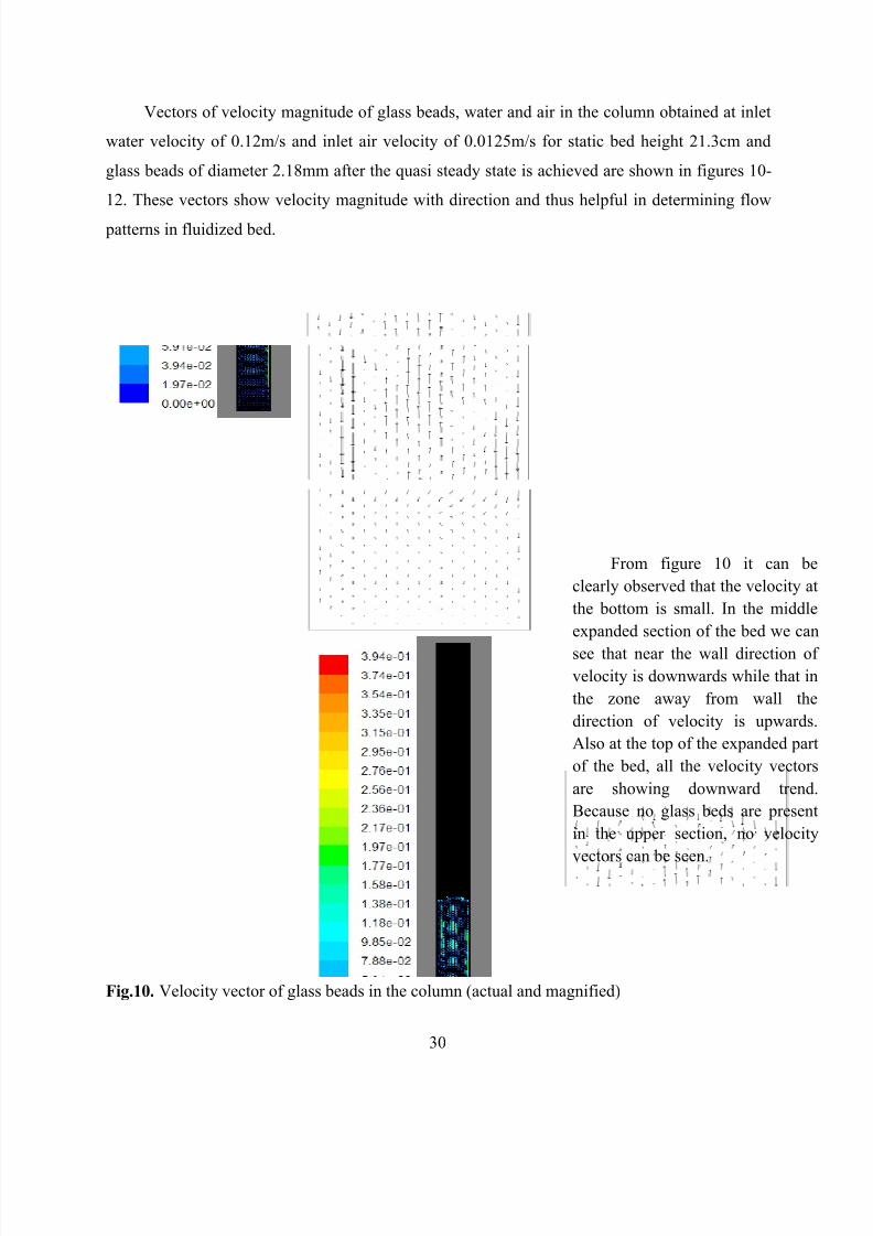
Vectors of velocity magnitude of glass beads, water and air in the column obtained at inlet
water velocity of 0.12m/s and inlet air velocity of 0.0125m/s for static bed height 21.3cm and
glass beads of diameter 2.18mm after the quasi steady state is achieved are shown in figures 10-
12. These vectors show velocity magnitude with direction and thus helpful in determining flow
patterns in fluidized bed.
Fig.10. Velocity vector of glass beads in the column (actual and magnified)
From figure 10 it can be
clearly observed that the velocity at
the bottom is small. In the middle
expanded section of the bed we can
see that near the wall direction of
velocity is downwards while that in
the zone away from wall the
direction of velocity is upwards.
Also at the top of the expanded part
of the bed, all the velocity vectors
are showing downward trend.
Because no glass beds are present
in the upper section, no velocity
vectors can be seen.
7/28/2019 CFD Modeling of Gas-Liquid-Solid Fluidized Bed
http://slidepdf.com/reader/full/cfd-modeling-of-gas-liquid-solid-fluidized-bed 40/57
31
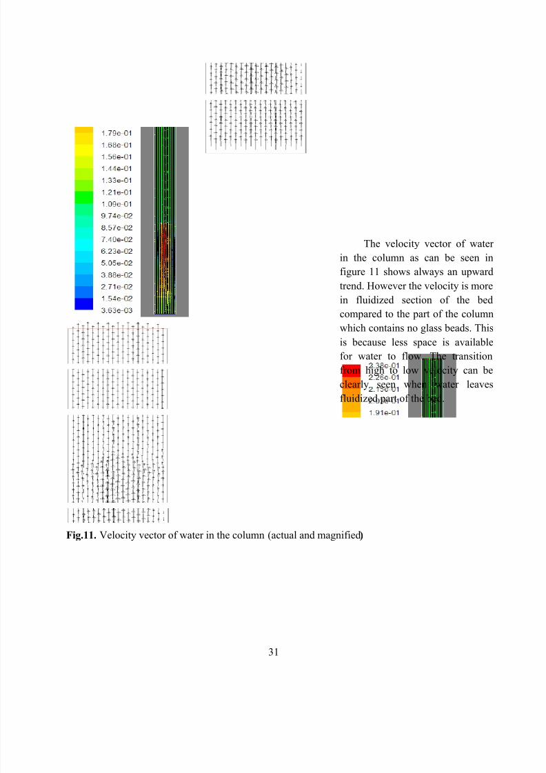
Fig.11. Velocity vector of water in the column (actual and magnified)
The velocity vector of water
in the column as can be seen in
figure 11 shows always an upwardtrend. However the velocity is more
in fluidized section of the bed
compared to the part of the column
which contains no glass beads. This
is because less space is available
for water to flow. The transition
from high to low velocity can be
clearly seen when water leaves
fluidized part of the bed.

7/28/2019 CFD Modeling of Gas-Liquid-Solid Fluidized Bed
http://slidepdf.com/reader/full/cfd-modeling-of-gas-liquid-solid-fluidized-bed 41/57
32
Fig.12. Velocity vector of air in the column (actual and magnified)
Here as it can be seen in
figure 12 the velocity vectors show
that velocity of air is very small in
fluidized portion of the column
compared to that in remaining part
of the column. This is because of
very small volume fraction of air
compared to glass beads and water.
This may also happen that glass beads obstruct the air bubbles
thereby lowering its velocity. In the
upper section of the column; water,
whose velocity is high carries air
bubbles, so velocity of air bubbles
reduces.

7/28/2019 CFD Modeling of Gas-Liquid-Solid Fluidized Bed
http://slidepdf.com/reader/full/cfd-modeling-of-gas-liquid-solid-fluidized-bed 42/57
33
Following are the XY plots of velocity magnitudes obtained at inlet water velocity of
0.12m/s and inlet air velocity of 0.0125m/s. For a fully developed flow this kind of parabolic
pattern is must. Besides, following figures also gives maximum outlet velocity of water about
0.14m/s and that of air about 0.48m/s. Also velocities at wall are zero.
Fig.13. XY plot of velocity magnitude of water
Fig.14. XY plot of velocity magnitude of air
7/28/2019 CFD Modeling of Gas-Liquid-Solid Fluidized Bed
http://slidepdf.com/reader/full/cfd-modeling-of-gas-liquid-solid-fluidized-bed 43/57
34
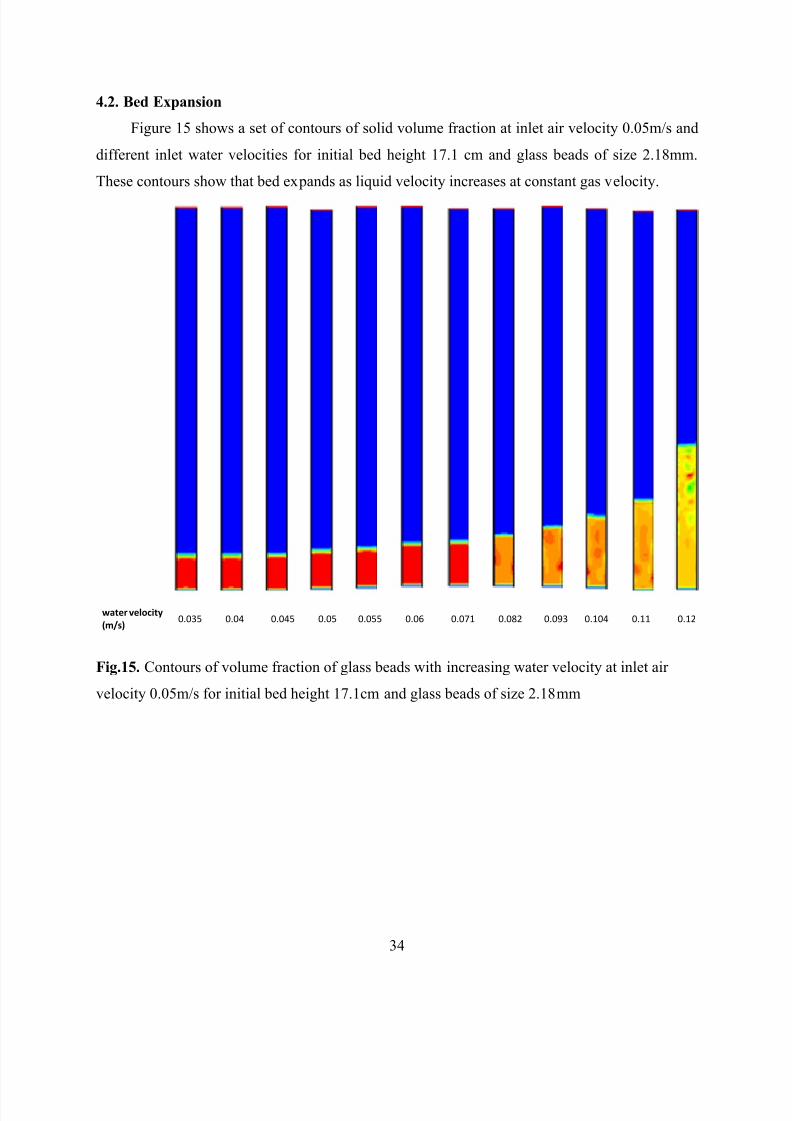
4.2. Bed Expansion
Figure 15 shows a set of contours of solid volume fraction at inlet air velocity 0.05m/s and
different inlet water velocities for initial bed height 17.1 cm and glass beads of size 2.18mm.
These contours show that bed expands as liquid velocity increases at constant gas velocity.
water velocity
(m/s)0.035 0.04 0.045 0.05 0.055 0.06 0.071 0.082 0.093 0.104 0.11 0.12
Fig.15. Contours of volume fraction of glass beads with increasing water velocity at inlet air
velocity 0.05m/s for initial bed height 17.1cm and glass beads of size 2.18mm

7/28/2019 CFD Modeling of Gas-Liquid-Solid Fluidized Bed
http://slidepdf.com/reader/full/cfd-modeling-of-gas-liquid-solid-fluidized-bed 44/57
35
Bed height is determined by taking an X-Y plot of volume fraction of glass beads on Y-
axis while height of the column at X-axis. Example:
Fig.16. X-Y plot of volume fraction of glass beads
Following are the trends of bed expansion vs. inlet water velocity obtained at different inlet
air velocities, which show that bed expands when water velocity increases.

7/28/2019 CFD Modeling of Gas-Liquid-Solid Fluidized Bed
http://slidepdf.com/reader/full/cfd-modeling-of-gas-liquid-solid-fluidized-bed 45/57
36
Fig.17. Bed expansion vs. water velocity for initial bed height 17.1cm and particle size 2.18mm
Fig.18. Bed expansion vs. water velocity for initial bed height 21.3cm and particle size 2.18mm
Next is shown a comparison of experimental results and simulated results obtained at air
velocity 0.05m/s and initial bed height 17.1 cm. It is clear that simulated results are in excellent
agreement with experimental results and there is hardly a difference of 1% or so.

7/28/2019 CFD Modeling of Gas-Liquid-Solid Fluidized Bed
http://slidepdf.com/reader/full/cfd-modeling-of-gas-liquid-solid-fluidized-bed 46/57
37
Fig.19. Comparison of experimental results and simulated results obtained at air velocity
0.05m/s and initial bed height 17.1 cm
4.3. Gas Holdup
Gas holdup is obtained as mean area-weighted average of volume fraction of air at
sufficient number of points in fluidized part of the bed. As shown in the adjoining figure 20
volume fraction of air phase is not the same at all points in fluidized part of the column. Hence
area weighted average of volume fraction of air is determined at heights 10cm, 20 cm 30 cm etc
till fluidized part is over. When these values are averaged gives the required gas holdup.
7/28/2019 CFD Modeling of Gas-Liquid-Solid Fluidized Bed
http://slidepdf.com/reader/full/cfd-modeling-of-gas-liquid-solid-fluidized-bed 47/57
38
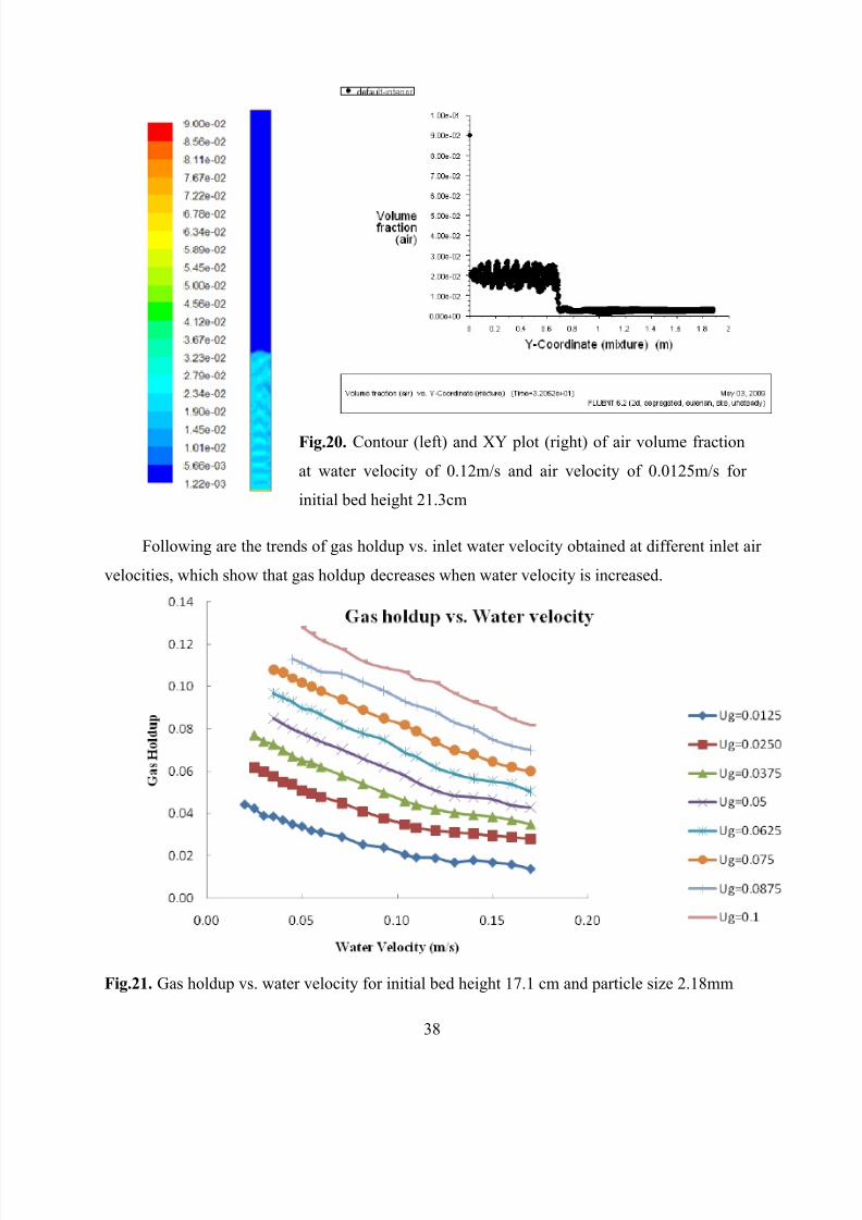
Following are the trends of gas holdup vs. inlet water velocity obtained at different inlet air
velocities, which show that gas holdup decreases when water velocity is increased.
Fig.21. Gas holdup vs. water velocity for initial bed height 17.1 cm and particle size 2.18mm
Fig.20. Contour (left) and XY plot (right) of air volume fraction
at water velocity of 0.12m/s and air velocity of 0.0125m/s for
initial bed height 21.3cm

7/28/2019 CFD Modeling of Gas-Liquid-Solid Fluidized Bed
http://slidepdf.com/reader/full/cfd-modeling-of-gas-liquid-solid-fluidized-bed 48/57
39
Fig.22. Gas holdup vs. water velocity for initial bed height 21.3 cm and particle size 2.18mm
Following are the trends of gas holdup vs. inlet air velocity obtained at different inlet water
velocities, which show that gas holdup increases when air velocity is increased.
Fig.23. Gas holdup vs. water velocity for initial bed height 17.1 cm and particle size 2.18mm

7/28/2019 CFD Modeling of Gas-Liquid-Solid Fluidized Bed
http://slidepdf.com/reader/full/cfd-modeling-of-gas-liquid-solid-fluidized-bed 49/57
40
Fig.24. Gas holdup vs. air velocity for initial bed height 21.3 cm and particle size 2.18mm
Following is the plot showing comparison of experimental result of gas holdup with that of
simulated result obtained at air inlet velocities 0.025 m/s and 0.05m/s for initial bed height 21.3
cm. It shows that in both the conditions simulated results are in excellent agreement with
experimental results with deviation of less than 5%. The reason for small deviation may be that
the glass beads used in experiment have a range of diameters while in the simulation all glass
beads are taken to be of the same diameter.
Fig.25. Comparison of experimental result of gas holdup with that of simulated result obtained at
air inlet velocities 0.025 m/s and 0.05m/s for initial bed height 21.3 cm

7/28/2019 CFD Modeling of Gas-Liquid-Solid Fluidized Bed
http://slidepdf.com/reader/full/cfd-modeling-of-gas-liquid-solid-fluidized-bed 50/57
41
4.4. Pressure Drop
Following are the contours of static gauge pressure (mixture phase) in the column obtained
at water velocity of 0.12m/s and air velocity of 0.0125m/s. This contour illustrates that pressure
increases as we move from top to bottom. Also pressure at inlet and outlet can be determined
which is helpful in finding the pressure drop across the column.
Following are the trends of pressure drop vs. water velocity obtained at different inlet air
velocities, which show that pressure drop increases when water velocity is increased. Also when
the air velocity is small (Ug=0.0125 m/s) there is no substantial increase in pressure drop. This
can be attributed to the fact that at small air velocity, the operation becomes almost solid-liquid
Fig.26. Contours of static gauge
pressure (mixture phase) in the
column obtained at water velocity
of 0.12m/s and air velocity of
0.0125m/s.

7/28/2019 CFD Modeling of Gas-Liquid-Solid Fluidized Bed
http://slidepdf.com/reader/full/cfd-modeling-of-gas-liquid-solid-fluidized-bed 51/57
42
fluidization because of small inlet volume fraction of the air compared to that of water.
Fig.27. Pressure Drop vs. water velocity for initial bed height 17.1 cm and particle size 2.18mm
Fig.28. Pressure Drop vs. water velocity for initial bed height 21.3 cm and particle size 2.18 mm
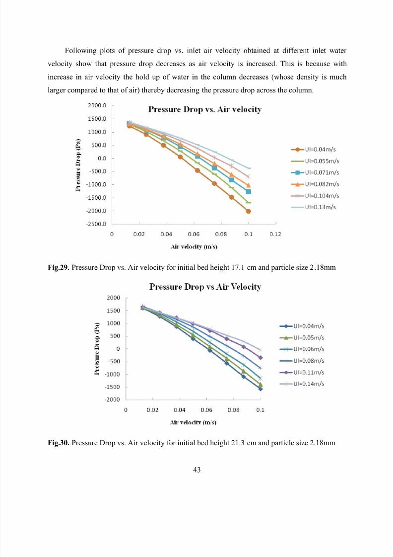
7/28/2019 CFD Modeling of Gas-Liquid-Solid Fluidized Bed
http://slidepdf.com/reader/full/cfd-modeling-of-gas-liquid-solid-fluidized-bed 52/57
43
Following plots of pressure drop vs. inlet air velocity obtained at different inlet water
velocity show that pressure drop decreases as air velocity is increased. This is because with
increase in air velocity the hold up of water in the column decreases (whose density is much
larger compared to that of air) thereby decreasing the pressure drop across the column.
Fig.29. Pressure Drop vs. Air velocity for initial bed height 17.1 cm and particle size 2.18mm
Fig.30. Pressure Drop vs. Air velocity for initial bed height 21.3 cm and particle size 2.18mm

7/28/2019 CFD Modeling of Gas-Liquid-Solid Fluidized Bed
http://slidepdf.com/reader/full/cfd-modeling-of-gas-liquid-solid-fluidized-bed 53/57
44
Following is shown a comparison between pressure drop from experiment and that from
simulation at air inlet velocity 0.025 m/s and 0.025 m/s for initial bed height 21.3 cm. The results
obtained from simulation differ from experiment only by 10% or less. The reason for this small
deviation may be that the glass beads used in experiment have a range of diameters while in the
simulation all glass beads are taken to be of the same diameter.
Fig.31. Comparison between pressure drop from experiment and that from simulation at air inlet
velocity 0.025 m/s and 0.025 m/s for initial bed height 21.3 cm

7/28/2019 CFD Modeling of Gas-Liquid-Solid Fluidized Bed
http://slidepdf.com/reader/full/cfd-modeling-of-gas-liquid-solid-fluidized-bed 54/57
45
CHAPTER 5
CONCLUSION
1. Trends of bed expansion vs. inlet water velocity obtained at different inlet air velocities
show that bed expands when water velocity increases.
2. Trends of gas holdup vs. inlet water velocity obtained at different inlet air velocities
show that gas holdup decreases when water velocity is increased.
3. Trends of gas holdup vs. inlet air velocity obtained at different inlet water velocities
show that gas holdup increases when air velocity is increased.
4. Trends of pressure drop vs. water velocity obtained at different inlet air velocities show
that pressure drop increases when water velocity is increased. Also when the air velocity is small
(Ug=0.0125 m/s) there is no substantial increase in pressure drop. This can be attributed to the
fact that at small air velocity, the operation becomes almost solid-liquid fluidization because of
small inlet volume fraction of the air compared to that of water.
5. Plots of pressure drop vs. inlet air velocity obtained at different inlet water velocity show
that pressure drop decreases as air velocity is increased. This is because with increase in air
velocity the hold up of water in the column decreases (whose density is much larger compared to
that of air) thereby decreasing the pressure drop across the column.
6.The pressure drop is influenced by the initial static bed height. This is low for small
initial bed height compared to higher initial bed height.
7. Since the bed expansion, gas holdup and pressure drop data obtained from simulation are
showing very small deviation from experimental results, therefore CFD model developed in this
work can be taken as very good approximation of gas-liquid-solid fluidized bed.

7/28/2019 CFD Modeling of Gas-Liquid-Solid Fluidized Bed
http://slidepdf.com/reader/full/cfd-modeling-of-gas-liquid-solid-fluidized-bed 55/57
46
References:
1. L. S. Fan, Gas – Liquid – Solid Fluidization Engineering, Butterworth-Heinemann, Boston, 1989
2. Bigot, V., Guyot I. Bataille D., Roustan M., "Possibilities of use of two sensors depression
metrological techniques and fiber optics, to characterize the hydrodynamics of a fluidised bed
triphasic", In: Stork, A., Wild, G. (Eds.), Recent Advances in Process Engineering, vol. 4 (1990).
pp. 143-1
3. Merchant F.J.A., Margaritis A., Wallace J.B., "A novel technique for measuring solute
diffusivities in entrapment matrices used in immobilization", Biotechnology and Bioengineering
30 (1987), 936 – 945.
4. Lauren A. Briens, Naoko Ellis, " Hydrodynamics of three-phase fluidized bed systems
examined by statistical, fractal, chaos and wavelet analysis methods", Chemical Engineering
Science 60 (2005) 6094 – 6106
5. Luo X., Jiang P., Fan L.S. "High-pressure three-phase fluidization: hydrodynamics and heat
transfer", A.I.Ch.E. Journal, 43 (1997), 2432 – 2445.
6. V.K. Bhatia and N. Epstein, "Three-phase fluidization: a generalized wake model
", In: H. Angelino, J.P. Couderc, H. Gibert and H. Lagueric, Editors, "Proceedings of the
International Symposium on Fluidization, Its Application", Cepadues-Editions, Toulouse (1974),
pp. 380 – 392
7. Jack T. Cornelissena, Fariborz Taghipoura, Renaud Escudiéa, Naoko Ellis, John R. Gracea,
―CFD modelling of a liquid–solid fluidized bed‖, Chemical Engineering Science 62 (2007) 6334
– 6348.
8. H.M. Jena, G.K. Roy, K.C. Biswal, "Studies on pressure drop and minimum fluidization
velocity of gas – solid fluidization of homogeneous well-mixed ternary mixtures in un-promoted
and promoted square bed", Chemical Engineering Journal 145 (2008) 16 – 24
9. Rigby G.R., VanBrokland G.P., Park W.H., Capes C.E. "Properties of bubbles in three-phase
fluidized bed as measured by an electro resistivity probe", Chemical Engineering Science 25
(1970), 1729 – 1741.

7/28/2019 CFD Modeling of Gas-Liquid-Solid Fluidized Bed
http://slidepdf.com/reader/full/cfd-modeling-of-gas-liquid-solid-fluidized-bed 56/57
47
10. Lee S.L.P., DeLasa, H.I. "Phase holdups in three-phase fluidized beds." A.I.Ch.E. Journal 33
(1987), 1359 – 1370.
11. Larachi F., Cassanello M., Chaouki J., Guy C. "Flow structure of the solids in a 3-D gas –
liquid – solid fluidized bed." A.I.Ch.E.Journal42 (1996), 2439 – 2452.
12. Muroyama, K. and L.S. Fan, ―Fundamentals of Gas-Liquid-Solid Fluidization‖, AIChE.J.
Vol.3, No.1, (1985), 1-34
13. Fraguío, M.S., Cassanello M.C., Larachi F.,Chaouki,J. "Flow regime transition pointers in
three-phase fluidized beds inferred from a solid tracer trajectory", Chemical
EngineeringandProcessing45 (2006), 350 – 358.
14. Dudukovic M.P., Devanathan N., Holub R. "Multiphase reactors Models and experimental
verification", Revuedel' Institute Francais du Petrole; 46 (1991),439 – 465.
15. Kulkarni A.A., Ekambara K., Joshi,J.B., "On the development of flow pattern in a bubble
column reactor: experiments and CFD", Chemical Engineering Science; 62 (2007), 1049 – 1072.
16. Cheung S.C.P., Yeoh G.H., Tu J.Y. "On the numerical study of isothermal vertical bubbly
flow using two population balance approaches", Chemical Engineering Science 62 (2007), 4659 –
4674.
17. Panneerselvam R., Savithri S., SurenderG.D. "CFD based investigations on hydrodynamicsand energy dissipation due to solid motion in liquid fluidized bed", Chemical Engineering
Journal132 (2007), 159 – 171.
18. Jiradilok, V.,Gidaspow,D.,Breault,R.W. "Computation of gas and solid dispersion
coefficients in turbulent risers and bubbling beds", Chemical Engineering Science62 (2007),
3397 – 3409.
19. Matonis, D.,Gidaspow,D.,Bahary,M., "CFD simulation of flow and turbulence in a slurry
bubble column", A.I.Ch.E.Journal 48 (2007), 1413 – 1429.
20. Feng W., Wen J., Fan J., Yuan Q., Jia X., Sun Y. "Local hydrodynamics of gas – liquid – nano
particles three-phase fluidization", Chemical Engineering Science 60 (2005), 6887 – 6898.

7/28/2019 CFD Modeling of Gas-Liquid-Solid Fluidized Bed
http://slidepdf.com/reader/full/cfd-modeling-of-gas-liquid-solid-fluidized-bed 57/57
21. Schallenberg J., En J.H., Hempel D.C. "The important role of local dispersed phase hold-up
for the calculation of three-phase bubble columns", Chemical Engineering Science 60 (2005),
6027 – 6033.
22. S. Ravelli_, A. Perdichizzi, G. Barigozzi. "Description, applications and numerical modellingof bubbling fluidized bed combustion in waste-to-energy plants", Progress in Energy and
Combustion Science 34 (2008) 224 – 253.
23. Shih TH, Liou WW, Shabbir A, Yang Z, Zhu J." A new k – ε eddy viscosity model for high
Reynolds number turbulent flows — model development and validation", Comput Fluids 24
(1995), 227 – 38
24. Srujal Shah, Lappeenranta University of Technology, "Theory and Simulation of Dispersed-
Phase Multiphase Flows", 07 May, 2008
25. Kunii D., Levenspiel O., Fluidization Engineering, 2nd Edition, ISBN: 0-409-90233-0, 1991.
26. L. S. Fan, Gas – Liquid – Solid Fluidization Engineering, Butterworth-Heinemann, Boston,
1989
27. Documentation, FLUENT 6.2, 2008.
28. FLUENT user‘s guide, vols. 1– 5. Lebanon, 2001.